Interaction of AMOC and intrinsic multidecadal Southern Ocean variability

A strongly-eddying version (0.1° horizontal resolution) of the Parallel Ocean Program (POP) shows pronounced intrinsic multidecadal variability in the Southern Ocean, the so-called Southern Ocean Mode (SOM). This Southern Ocean multidecadal variability is induced by eddy-mean flow interaction and deep convection. The SOM variability propagates through the global ocean and influences the strength of the Atlantic Meridional Overturning Circulation (AMOC) by about 3 Sv. The opposite role on how the AMOC influences the SOM is unknown, as this requires long simulations and preferably with different AMOC background states. Here, using the results of a simulated AMOC collapse in the strongly-eddying ocean-only POP version, we find that the amplitude of the SOM is substantially reduced following an AMOC collapse. Associated changes in horizontal and vertical density variations lead to a weakening of the Antarctic Circumpolar Current transport and a shutdown of deep convection in the Weddell Sea. In contrast, these changes promote deep convection events and the emergence of multidecadal variability in the Pacific sector of the Southern Ocean. A mechanical energy budget analysis shows both a reduction in the wind input and a disruption of the phase difference between wind work and the potential to kinetic energy conversion. The results highlight the strong connection between the AMOC and intrinsic multidecadal variability in the Southern Ocean.

1 Introduction

Although observations are limited, there is now more and more evidence for the existence of multidecadal variability in the Southern Ocean. For example, signatures of such variability have been identified in sea surface temperatures (SSTs) (Latif et al., 2013; Fan et al., 2014; Dalaiden et al., 2025), and are connected to polynya formation in the Weddell Sea (Latif et al., 2017; Zhou et al., 2025). Furthermore, paleoclimate data assimilation based reconstructions of Antarctic sea-ice anomalies over the period 1700–2000 (Dalaiden et al., 2023, 2025) indicate significant multidecadal variability with dominant periods of 40–50 and 80–100 years (Morioka et al., 2024).

Models that participated in the most recent Climate Model Intercomparison Projects (CMIP5 and CMIP6) have simulated multidecadal variability in the Southern Ocean. In a 2000 years pre-industrial control simulation of the SPEAR (GFDL) model, multidecadal variability in the strength of the Antarctic Bottom Water cell is found (Zhang et al., 2019). The subsequent initialization phases of the model for the historical period, in particular related to convective activity, are shown to be important to explain recent trends in Antarctic sea ice. The 3000 years simulations of two versions of the SPEAR model (having different atmospheric resolutions) also display significant multidecadal variability with dominant time scales around 95 years (Morioka et al., 2024). The multidecadal variability in these models is explained (Morioka et al., 2024) by the interaction of the Southern Annular Mode (SAM) and ocean deep convection. Stronger westerlies enhance upwelling of relatively warm and saline (subsurface) water that weakens the upper ocean stratification, inducing convection. This then mixes more saline and warm water in the upper layer, in a typical Welander salinity-convective feedback (Welander, 1982). Another mechanism which has been suggested is a teleconnection with El Niño variability, through the propagation of Rossby waves (Chang et al., 2020; Wang et al., 2022).

While the effects of ocean eddies were parameterised in the models mentioned above, it was shown that when strongly-eddying ocean models are used, a new mode of multidecadal variability appears (Le Bars et al., 2016; van Westen and Dijkstra, 2020; Chang et al., 2020; Diao et al., 2022). In the ocean-only version of the Parallel Ocean Program (POP), this variability was named (Le Bars et al., 2016) the Southern Ocean Mode (SOM). The effects of the SOM extend into the North Atlantic, where it induces a ∼3 Sv ($\mathrm{1}\mathrm{Sv}={\mathrm{10}}^{\mathrm{6}}{\mathrm{m}}^{\mathrm{3}}{\mathrm{s}}^{-\mathrm{1}}$) variability in the strength of the Atlantic Meridional Overturning Circulation (AMOC) at 26° N. The mechanism of the SOM was analysed in Jüling et al. (2018) by investigating its Lorenz Energy Cycle (LEC). Clear support was found for a mechanism suggested earlier by Hogg and Blundell (2006), where enhanced baroclinic instability in the Antarctic Circumpolar Current (ACC) region affects the mechanical energy input by the wind through a decrease of the zonality of the jet. This weakens the ACC and hence also eddy formation, leading to a more zonal jet, thereby closing the cycle. This also explains the absence of the SOM in the non-eddying version of the POP (van Westen et al., 2025), as the explicit representation of ocean eddies is required for this mechanism (Jüling et al., 2018; Le Bars et al., 2016). Apart from this eddy-mean flow interaction mechanism, deep convection in the Weddel Gyre region is also modified along this cycle, and it turned out to be difficult to determine whether it plays an active or passive role in the SOM mechanism (Jüling et al., 2018; Ford et al., 2026).

While the SOM induces variability of the AMOC at 26° N, the role of the AMOC in the existence of the SOM has not been studied. Very recently, a quasi-equilibrium freshwater flux forcing simulation was performed using the same strongly-eddying POP model as in Le Bars et al. (2016), showing that the AMOC collapses to a weak state of about 5 Sv (van Westen et al., 2025). This simulation provides an opportunity to study the AMOC-SOM connection in more detail, which is the aim of this paper. Our main focus is on how a large decrease in AMOC strength modifies the density field in the Southern Ocean, the ACC, deep convection and the properties of the SOM. Given the strong coupling between intrinsic Southern Ocean variability and key climate processes, such as Antarctic sea-ice variability (Gwyther et al., 2018; Morioka et al., 2022; Hobbs et al., 2024), oceanic heat and carbon uptake (Mayewski et al., 2009; Wendt et al., 2024), and teleconnections to other modes of variability (van Westen and Dijkstra, 2017), the results of this study are relevant for interpreting past, present and future Southern Ocean multidecadal climate variability.

2 Methods

2.1 Ocean model simulations

We use output from the quasi-equilibrium freshwater forcing simulation performed by van Westen et al. (2025) using a strongly-eddying configuration of the Parallel Ocean Program (POP, version 2) (Dukowicz and Smith, 1994), with a nominal horizontal resolution of 0.1° and 42 non-equidistant vertical levels. The model is forced using observed river run-off fields and a prescribed atmospheric state based on the repeat annual cycle (normal year) Coordinated Ocean Reference Experiment (CORE) forcing data set (Large and Yeager, 2004), with 6 hourly forcing averaged to a monthly resolution. Precipitation is also taken from the CORE forcing dataset. Wind stress is computed offline using the Hurrell SST climatology (Hurrell et al., 2008) and standard bulk formulae, whereas evaporation and sensible heat flux are calculated online using the model prescribed SST and bulk formulae. A diagnosed freshwater flux, determined from an equilibrium spin-up, is also prescribed. Sea-ice cover is prescribed based on the −1.8 °C isoline of the SST climatology, with both temperature and salinity restored on a timescale of 30 d under diagnosed climatological ice (Weijer et al., 2012). Apart from this, there is no salinity restoring in the model. Details on model configuration and simulation procedure can be found in the Supplementary Material of Weijer et al. (2012).

The quasi-equilibrium freshwater flux forcing simulation in van Westen et al. (2025) was initialised from model year 300 of the multi-century simulation performed by Le Bars et al. (2016). Model drift is still present (van Westen et al., 2026), but occurs on much longer timescales than the AMOC decline. From the start of the quasi-equilibrium simulation, a freshwater flux with strength F_H is applied over the North Atlantic sector (20–50° N) with a constant rate of $\mathrm{3}\times {\mathrm{10}}^{-\mathrm{4}}\mathrm{Sv}{\mathrm{yr}}^{-\mathrm{1}}$, similar to the hosing simulation performed in the Community Earth System Model (CESM) (van Westen and Dijkstra, 2023). The freshwater flux anomaly is globally compensated to conserve salinity. The AMOC strength is weakening under increasing F_H values and collapses around F_H=0.125 Sv (model year 415); more details on this simulation can be found in van Westen et al. (2025).

2.2 The Southern Ocean Mode (SOM)

In the simulations of Le Bars et al. (2016), the temperature anomalies associated with the SOM (see their Fig. 2) propagate eastward along the ACC in the South Atlantic, where they are disrupted south of Africa around 30° E due to the interaction with the Agulhas Current Retroflection (Le Bars et al., 2016). The anomalies then split into two pathways, where one continues along the ACC and slowly dissipates, while the other enters the Weddell Gyre, likely due to enhanced cross-stream eddy diffusivity compared to the South Atlantic (Sallée et al., 2008). The heat anomalies also propagate northward through the Atlantic basin, thereby inducing multidecadal variations in the AMOC strength up to 3 Sv. The SOM is associated with a peak-to-peak variability of approximately 60 ZJ (1 ZJ≡10²¹ J) in global ocean heat content (OHC), highlighting its potential significance for large-scale climate variability.

Although the spatial pattern of the SST anomalies associated with the SOM extends across the entire Southern Ocean, the largest anomalies can be found in the South Atlantic sector (Le Bars et al., 2016). To quantify this variability, it is measured using the SOM index, which is defined as the SST anomaly averaged over the region 50–35° S, 0–50° W (black outlined region in Fig. 2a).

2.3 Energetics of the SOM

Previous studies have analysed the mechanical energy budget of the SOM in the POP control simulation (Le Bars et al., 2016; Jüling et al., 2018). It was shown that eddy-mean flow interactions are central to explain the SOM, similar to that of a mode of multidecadal variability identified in a three-layer, eddy-resolving, quasi-geostrophic model of a zonal channel flow (Hogg and Blundell, 2006). The oscillatory behaviour arises from phase lags between mechanical energy input by the wind, generation of eddies by baroclinic instability, and the zonality of the mean flow. Below, we also apply a similar mechanical energy budget analysis to the quasi-equilibrium POP simulation to investigate the effects of an AMOC weakening on the SOM.

The Lorenz Energy Cycle (LEC) framework (von Storch et al., 2012) has proven effective for analysing the multidecadal variability of the SOM (Jüling et al., 2018). Further simplifications of the full LEC framework have been proposed by Sinha and Abernathey (2016), and these have been successfully applied to the POP model output to explain the oscillatory behaviour of the SOM (Jüling et al., 2020). In the following, we denote K, K_m, K_e as the volume-integrated total kinetic energy, mean kinetic energy and eddy kinetic energy, respectively; and P, P_m and P_e as the volume-integrated available potential energy, mean available potential energy and eddy available potential energy, respectively.

The total kinetic energy K is computed according to:

$$\begin{array}{}\text{(1)}& K={\displaystyle \frac{{\mathit{\rho }}_{\mathrm{0}}}{\mathrm{2}}}\underset{V}{\int }\left(\stackrel{\mathrm{‾}}{u^{\mathrm{2}}+v^{\mathrm{2}}}\right)\mathrm{d}V,\end{array}$$

where $\mathit{u}=(u,v)$ denotes the horizontal velocity vector, ρ₀ the global average density of sea water, and V the volume over which the energetics are evaluated. The overbar represents a 5 year time average used to perform the eddy-mean decomposition, consistent with previous studies on the energetics of the SOM (Le Bars et al., 2016; Jüling et al., 2018). The results are not sensitive to small changes in the averaging window (tested for 3–10 year time averages). The mean kinetic energy is given by:

$$\begin{array}{}\text{(2)}& K_{\mathrm{m}}={\displaystyle \frac{{\mathit{\rho }}_{\mathrm{0}}}{\mathrm{2}}}\underset{V}{\int }({\stackrel{\mathrm{‾}}{u}}^{\mathrm{2}}+{\stackrel{\mathrm{‾}}{v}}^{\mathrm{2}})\mathrm{d}V,\end{array}$$

and the eddy kinetic energy is computed as the difference between K and K_m per gridpoint. The available potential energy is expressed as:

$$\begin{array}{}\text{(3)}& P=-{\displaystyle \frac{g}{\mathrm{2}}}\underset{V}{\int }{\displaystyle \frac{\mathrm{1}}{n_{\mathrm{0}}}}\stackrel{\mathrm{‾}}{{\mathit{\rho }}^{*\mathrm{2}}}\mathrm{d}V,\end{array}$$

where the potential density anomalies are defined as ${\mathit{\rho }}^{*}(x,y,z,t)=\mathit{\rho }(x,y,z,t)-{\mathit{\rho }}_{\text{ref}}\left(z\right),$ with ${\mathit{\rho }}_{\text{ref}}\left(z\right)=\langle \mathit{\rho }(x,y,z,t){\rangle }_{\text{av}}$ representing the global reference state (von Storch et al., 2012). In the expression for ρ_ref, the angled brackets indicate a global area average, while the subscript denotes a time average over one SOM cycle. Furthermore, g denotes the gravitational acceleration and n₀(z) the vertical gradient of the reference potential density. An eddy-mean decomposition can be performed to determine the mean and eddy potential energies (P_m and P_e, respectively). The analysis is conducted over the entire Southern Ocean south of 30° S (SO30 region), thereby capturing the complete SOM variability and avoiding problems of boundary terms (Jüling et al., 2018).

Under the approximations outlined in detail by Jüling et al. (2020), the evolution equations for the volume integrated eddy kinetic energy K_e and available potential energy P are given by:

$$\begin{array}{}\text{(4)}& {\displaystyle }& {\displaystyle \frac{\mathrm{d}P}{\mathrm{d}t}}\approx G\left(K_{\mathrm{m}}\right)-C(P_{\mathrm{e}},K_{\mathrm{e}})-D\left(K_{\mathrm{m}}\right),\text{(5)}& {\displaystyle }& {\displaystyle \frac{\mathrm{d}{K}_{\mathrm{e}}}{\mathrm{d}t}}\approx C(P_{\mathrm{e}},K_{\mathrm{e}})-D\left(K_{\mathrm{e}}\right).\end{array}$$

Here, the generation of mean kinetic energy by the wind forcing exerting a stress on the ocean surface S is expressed as:

$$\begin{array}{}\text{(6)}& G\left(K_{\mathrm{m}}\right)=\underset{S}{\int }(\stackrel{\mathrm{‾}}{{\mathit{\tau }}_x}\stackrel{\mathrm{‾}}{u}+\stackrel{\mathrm{‾}}{{\mathit{\tau }}_y}\stackrel{\mathrm{‾}}{v})\mathrm{d}S,\end{array}$$

with $\mathit{\tau }=({\mathit{\tau }}_x,{\mathit{\tau }}_y)$ the wind stress. The exchange of potential to eddy kinetic energy associated with baroclinic instability, C(P_e,K_e), is determined by:

$$\begin{array}{}\text{(7)}& C(P_{\mathrm{e}},K_{\mathrm{e}})=-g\underset{V}{\int }\stackrel{\mathrm{‾}}{{\mathit{\rho }}^{\prime }{w}^{\prime }}\mathrm{d}V\approx C(P,K)-C(P_{\mathrm{m}},K_{\mathrm{m}}),\end{array}$$

where w denotes the vertical velocity and the prime indicates anomalies with respect to the 5 year time average. The terms in the mechanical energy budget are calculated using 5 year moving averages, while eddy contributions are determined from monthly mean data. The terms D(X) above are dissipation terms, but are not crucial to study the SOM cycle (Jüling et al., 2018). The degree of non-zonality of the mean flow, which is a proxy for the baroclinic generation of eddies, is quantified by $\mathit{\zeta }=(\int \stackrel{\mathrm{‾}}{v^{\mathrm{2}}}\mathrm{d}V)/(\int \stackrel{\mathrm{‾}}{u^{\mathrm{2}}}\mathrm{d}V)$, where the squared meridional and zonal velocities are computed first and then volume integrated over the SO30 region and the top 300 m.

3 Results

3.1 Changing SOM variability

In the quasi-equilibrium simulation of the POP, a gradual increase in surface freshwater forcing leads to a weakening of the AMOC (Fig. 1a). The AMOC strength at 26° N decreases from a mean of 19.4 Sv during the first 50 model years to a mean of 4.8 Sv during the last 50 model years. The onset of the collapse occurs around model year 415 (van Westen et al., 2025). The SOM index (Fig. 1b, black curve) exhibits distinct multidecadal variability over the first 200 model years, with a dominant period of approximately 45 years that is statistically significant at the 95 % confidence level based on a Morlet wavelet power spectrum (Fig. A1b). As the freshwater forcing increases, this period becomes longer, reaching approximately 50 years between model years 300–500. After the AMOC collapse and over the last 100 model years, the variability in the SOM index disappears entirely (Fig. A1b). The Drake Passage transport (Fig. 1c) displays the same multidecadal variability as the SOM index over the first 300 years (Fig. A1a), with a peak-to-peak amplitude of about 17 Sv. Subsequently, the mean transport and the amplitude of multidecadal variability slightly decrease, the former by about 10 Sv and the latter being minimal just before the onset of the AMOC collapse. Interestingly, this amplitude increases again after the AMOC collapse, while the frequency of variability slightly decreases (Fig. A1a).

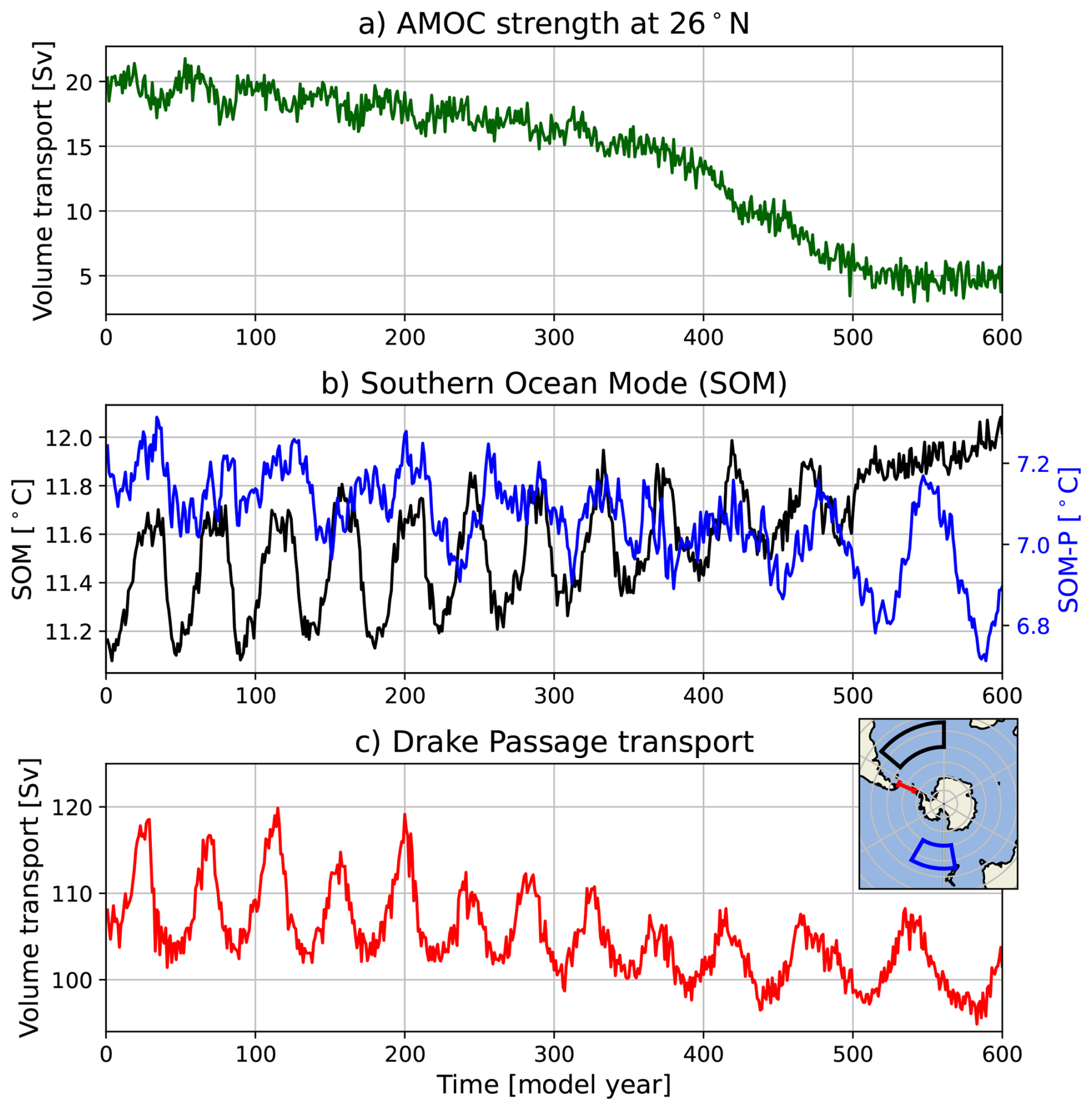
Figure 1 Results for the quasi-equilibrium, high-resolution POP simulation. Time series of (a): the AMOC strength at 1000 m depth and 26° N, (b): the SOM (black) and SOM-P (blue) index, and (c): the Drake Passage volume transport. The inset in panel c shows the black (blue) outlined region used to determine the SOM (SOM-P) index. The full-depth Drake Passage volume transport is determined over the red section (66–55° S, 66° W).

To understand the disappearing multidecadal variability in the AMOC strength time series, we conduct an empirical orthogonal function (EOF) analysis on annual mean SSTs south of 30° S for the first and last 100 model years of the simulation. All time series are first linearly detrended and normalised by their standard deviations, and subsequently weighted to their surface area prior to conducting the EOF analysis. The dominant EOF pattern and associated principle component (PC) are shown in Fig. 2. During the first 100 model years (Fig. 2a), the EOF exhibits relatively strong (negative) amplitudes over the Atlantic sector in the Southern Ocean. This motivates the choice of the region used for the SOM index (Le Bars et al., 2016), as indicated by the black outlined region (50–35° S, 0–50° W). The corresponding PC (Fig. 2c) exhibits a similar period to that of the SOM index, highlighting the dominance of this multidecadal variability in the SO30 region.

After the AMOC collapse (last 100 model years), the pattern of the EOF changes significantly, with the largest amplitudes now located in the Pacific sector of the Southern Ocean (Fig. 2b). The period of the associated PC increases to approximately 75 years (Fig. 2d), matching the period of the Drake Passage transport over the last 100 years (Fig. A1a). This motivates us to also study the variability in the Pacific sector, where we define the SOM-P index as the spatially-averaged SSTs over the blue outlined region (60–45° S, 170° E–150° W), which coincides with the region of largest EOF amplitudes (Fig. 2b). Interestingly, a pronounced mode of multi-decacal variability emerges in the SOM-P index only after the onset of the AMOC collapse around model year 415 (blue curve in Fig. 1b). The dominant period during the last 150 model years is approximately 75 years, and is statistically significant at the 95 % confidence level based on a Morlet wavelet power spectrum (Fig. A1c). The dominant period of the SOM-P index is consistent with that of the Drake Passage transport after the AMOC has collapsed (Fig. A1a). This suggests that Pacific variability is associated with the multidecadal behaviour of the Drake Passage transport after the AMOC has collapsed, as will be further explored below in Sect. 3.4.

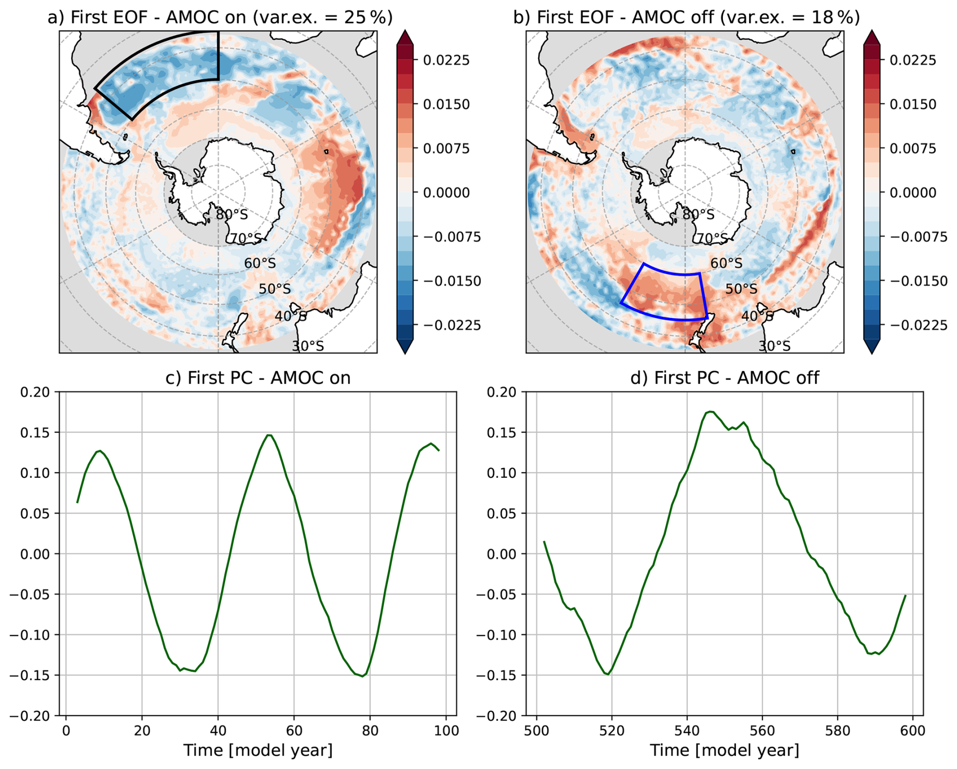
Figure 2 First EOFs of annual mean SSTs south of 30° S for the first 100 model years (a) and the last 100 model years (b), with the explained variance indicated. A moving average of 5 years has been applied to the data prior to the EOF analysis. The black (blue) outlined region shows the region used to determine the SOM (SOM-P) index. Panels (c, d) show the corresponding first PCs.

3.2 AMOC–SOM coupling

Density anomalies associated with the SOM propagate northward and submerge around 40° S (van Westen and Dijkstra, 2017), generating multidecadal variability in the subsurface temperature and salinity fields (Fig. A2). These subsurface anomalies continue to propagate northward within the Atlantic basin, thereby influencing the strength of the upper branch of the AMOC (van Westen and Dijkstra, 2017). As a result, the AMOC strength at 26° N exhibits a similar 45 year oscillation period as the SOM index during the first 300 model years (Fig. A3a). As the AMOC weakens, the distinct temperature and salinity patterns associated with the positive and negative phases of the SOM disappear (Fig. A2), and the AMOC loses its multidecadal variability (Fig. A3b).

The substantially weakened AMOC leads to a pronounced reduction in meridional heat and salinity transport (van Westen et al., 2025), resulting in an accumulation of heat and convergence of salt in the Southern Hemisphere ocean interior, extending to depths up to 1000 m north of the Antarctic subpolar front (50° S). This causes both warming (Fig. 3a) and salinification (Fig. 3b) of the subsurface waters, consistent with previous studies on a weakened AMOC (Weijer et al., 2019; van Westen et al., 2024; Diamond et al., 2025). In contrast, the deep waters experience a freshening and slight cooling related to the reduced formation of North Atlantic Deep Water (NADW), and a reorganization of the water masses in the Southern Ocean. The resulting density changes show an increase in the upper 1000 m between 50 and 20° S, and a decrease further north (Fig. 3c). At greater depths, the waters become less dense, primarily driven by salinity changes (Fig. A4).

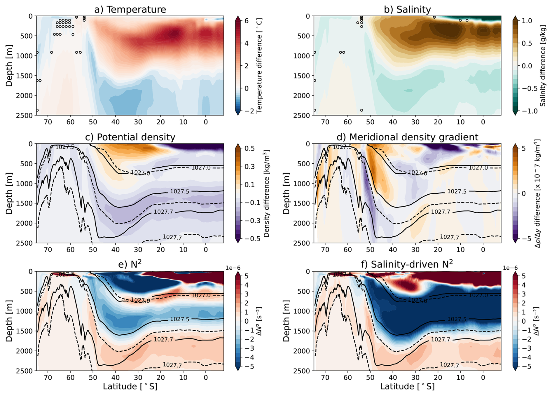
Figure 3 Temperature, salinity, density, meridional density gradient and buoyancy frequency (N²) differences in the Atlantic sector. Zonally averaged (60° W–25° E) (a) temperature, (b) salinity, (c) density, (d) meridional density gradient, (e) N², and (f) salinity-driven N² differences in the upper 2500 m before and after the AMOC collapse (model year (500–600) minus model year (1–100)). In (c–f), the solid (dashed) black lines denote isopycnals of model year 1–100 (500–600). Plotted isopycnals are (from top to bottom): 1027.0, 1027.5, and 1027.7 kg m⁻³ for model year 1–100 (500–600). The markers in panel a, b indicate non-significant (p≧0.05, two-sided Welch's test) differences, which are not shown in panels c–f to enhance visibility.

Between 50–40° S and over the upper 1000 m, the isopycnals slope downward and this is indicative of the Antarctic subpolar front (solid curves in Fig. 3c–f). This meridional density gradient becomes less negative after the AMOC collapse, resulting in a decrease of the isopycnal slope (shading and dashed curves in Fig. 3c). By contrast, a negative meridional density gradient difference is found at subsurface depths (1000–2000 m) and near 50° S, corresponding to a steepening of the isopycnals. Changes in the isopycnal slopes modify the baroclinicity, thereby influencing the strength of the ACC through thermal wind balance (Fig. 1c). The changes in the meridional density gradient are not uniform across the ACC latitude band (50° S - 40° S), and may therefore lead to spatially heterogeneous changes in the ACC. van Westen and Dijkstra (2020) showed that an increased meridional slope of the isopycnals near 50° S corresponds to a reduction of the SOM period in the CESM model. This is consistent with the results here, where an increase in the SOM period occurs simultaneously with the meridional isopycnal slopes becoming less negative (near 50° S and upper 1000 m).

The displacement of the isopycnals leads to changes in the stratification of the water masses (Fig. 3e), with clear bands of increased and decreased stratification. Stratification decreases in the water mass north of 50° S between 1000 and 1500 m, but, in contrast, waters below 1500 m and those that upwell south of 50° S show an overall increase in stratification. The latter increases are primarily driven by salinity-controlled changes in N² (Fig. 3f), while stratification changes north of 50° S and in the upper 1500 m result from a combination of temperature- and salinity-driven effects.

Similar to the Atlantic sector, the Indian and Pacific sectors of the Southern Ocean also exhibit warming and salinification over the upper 1000 m and north of 45° S (Figs. A5 and A6). These changes are accompanied by a decrease of the meridional density gradient over the near-surface layer, and an increase of this gradient in the subsurface layers across the ACC latitude band (between 50 and 40° S). Stratification weakens north of 60° S in the upper 1500 m, while deeper waters show an overall increase in stratification. The AMOC weakening therefore leads to a basin-wide reorganization of the Southern Ocean density structure, which appears to suppress SOM-related variability in the Atlantic sector while enabling the emergence of a new mode of multidecadal variability in the Pacific sector.

3.3 Mechanisms of SOM changes

To understand the reduced SOM variability after the AMOC collapse, we analysed the mechanical energy changes over the SO30 region. The dominant terms of the mechanical energy budget are evaluated over the full simulation period, and over three different SOM cycles: one early in the simulation (SOM cycle 1, model years 63–114), one during the AMOC collapse (SOM cycle 2, model years 410–480), and one during the weak AMOC state (SOM cycle 3, model years 500–600). The difference in cycle length reflects the increasing SOM (SOM-P) period under increasing freshwater flux forcing. The mechanical energy budget analysis is displayed in Fig. 4.

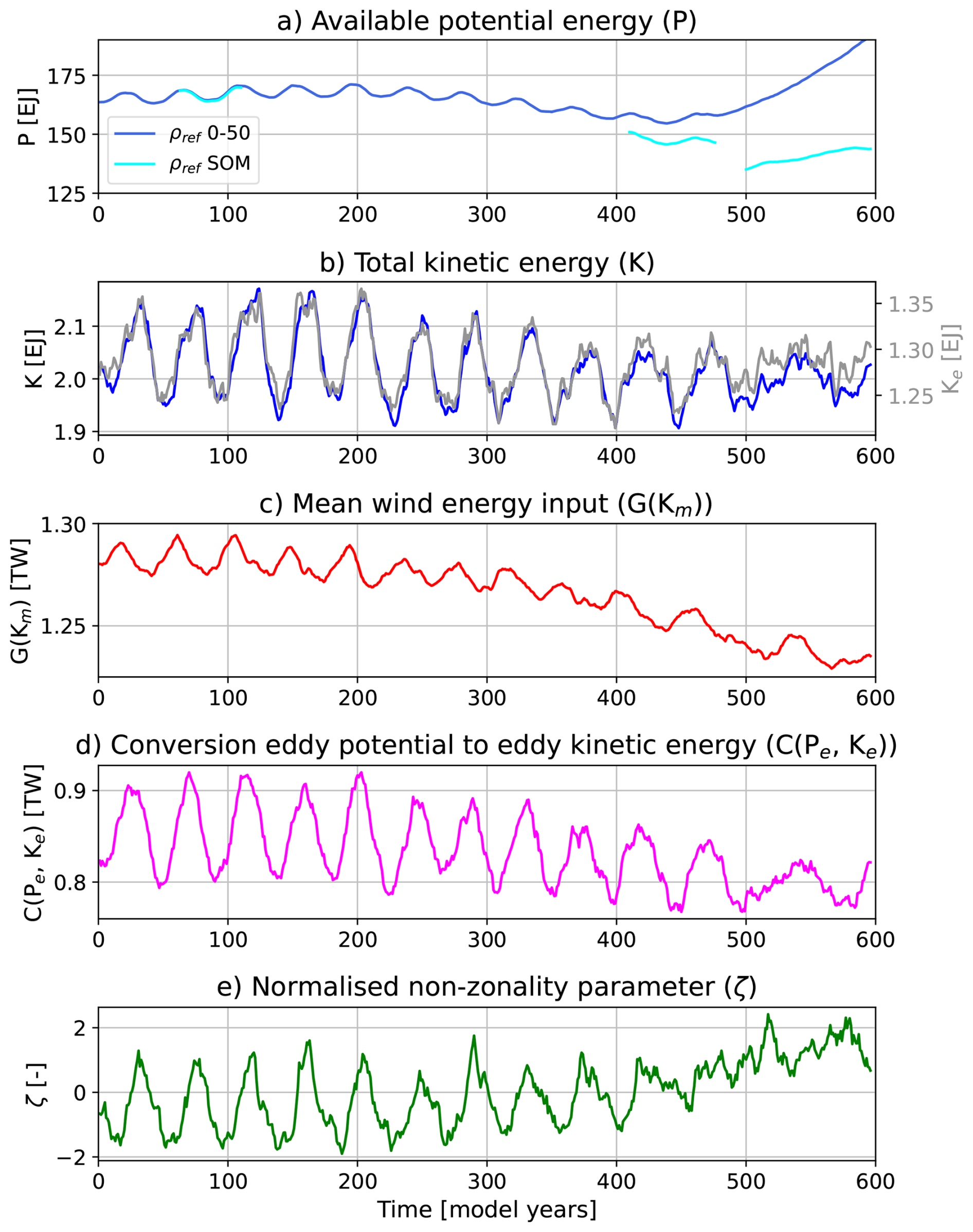
Figure 4 Energetics in the SO30 region. Time series of (a) volume integrated (90–30° S) available potential energy (P), (b) total kinetic energy (K), (c) energy conversion of eddy potential energy to eddy kinetic energy (C(P_e,K_e)), (d) mean energy input by the wind (G(K_m)) and (e) a measure of the normalised, mean-centered non-zonality of the flow field ζ. All time series represent 5 year running averages. In panel (a), the blue line represents the time series of P calculated with a reference density ρ_ref taken from the first 50 model years, whereas the cyan line uses a ρ_ref averaged over the corresponding SOM cycle.

The available potential energy, P, is dependent on the reference density ρ_ref used (see Eq. 3). We compute P over the full simulation using a fixed ρ_ref derived from the first 50 model years (dark blue curve in Fig. 4a), such that all changes in P reflect variations in the density structure rather than changes in the reference state. In contrast, P for the individual SOM cycles is computed using ρ_ref averaged over the corresponding SOM cycle period (cyan curves in Fig. 4a). The different choices of ρ_ref do influence the magnitude of P, but not their overall variability and tendency.

The available potential energy starts to increase in the SO30 region following the AMOC collapse, with the Atlantic, Indian, and Pacific sectors contributing approximately 29 %, 30 %, and 41 %, respectively, to the total P in this region. An increase in P indicates that the water column is further displaced from its stable reference state. This is also consistent with the decrease in vertical stratification in the upper 1500 m in the Atlantic, Indian and Pacific sectors south of 30° S, as shown in Fig. 5. The available potential energy, however, has not yet reached an equilibrium state at the end of the simulation, as P continues to increase.

The tendency of P (Fig. 4) is affected by the terms G(K_m), representing the mean wind energy input, and by C(P_e,K_e), representing conversion of eddy potential to eddy kinetic energy. An increase in G(K_m), e.g. due to a more zonal flow with steeper isopycnals, increases P. In contrast, an increase in C(P_e,K_e) reflects enhanced eddy generation through baroclinic instability, transferring more energy from P_e to K_e, and thus reduces P over time. Figure 4 shows both a mean reduction of G(K_m) and C(P_e,K_e), although the reduction in G(K_m) is larger (Fig. 4c and d). The increase in P at the end of the simulation is therefore not driven by enhanced mean wind energy input, but instead is a consequence of changes in the density field associated with the AMOC collapse. Additionally, K and K_e primarily exhibit a reduced amplitude of variability rather than a shift in mean magnitude (Fig. 4b).

The relatively zonal background ACC flow starts to meander more after the AMOC collapse, which is reflected in the increase of the non-zonality parameter (ζ, Fig. 4e). This increase is consistent with the reduction in mean wind energy input over time, as the correlation between the zonal wind forcing and the zonal mean flow weakens. While an increased non-zonal flow is typically associated with enhanced eddy activity, this is not reflected in an overall increase of C(P_e,K_e). The non-zonality parameter loses its multidecadal variability entirely after the AMOC collapse, suggesting that its increase is not primarily driven by variability in the eddy generation and mean wind energy input. Mean flow changes likely also play a role, e.g. a reduction in the mean ACC strength or a shift in its position could lead to increased meandering of the zonal flow.

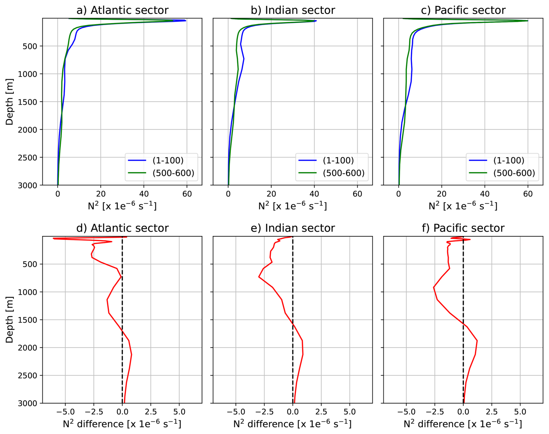
Figure 5 Depth profiles of the squared Brunt–Väisälä frequency (N²) area-averaged in the (a) Atlantic sector (60° W–25° E), (b) the Indian sector (25–150° E), and (c) the Pacific sector (150° E–60° W) of the Southern Ocean (90–30° S). (d–f): Similar to (a–c) but now showing the difference between model year (500–600) and (1–100).

Following the framework established in earlier studies (Hogg and Blundell, 2006; Le Bars et al., 2016; Jüling et al., 2018), the SOM cycle can be divided into four distinct regimes (Fig. 6a), where the vertical stratification plays a key role in setting the timescale of this SOM cycle (van Westen and Dijkstra, 2020). Note that the quantities are now centered (zero mean) and normalised by their standard deviation, to more clearly see the phase differences between the different terms. Regime A corresponds to a low-energy state with a relatively zonal ACC, starting at the minimum of the total potential energy P and ending at the minimum of the total kinetic energy K. In regime B, P increases as the zonal flow is accelerated by the wind work, leading to a maximum of P. Regime C represents the high-energy state, spanning from the maximum of P to the maximum of K. During this period, the flow undergoes enhanced baroclinic instability, leading to an increase in the generation of eddies by the mean flow. The P accumulated in regimes A and B is now converted to eddy kinetic energy. This enhanced eddying flow rearranges the flow field, making it less zonal, thereby disrupting the correlation between the surface ocean velocity and the wind stress. As a result, the wind energy input quickly decreases. Finally, regime D is characterised by declining P and K. As the storage of P becomes exhausted, the conversion of P to K begins to diminish as well. This, combined with the reduction in wind work, drives the flow back to its low-energy state, thereby completing the cycle.

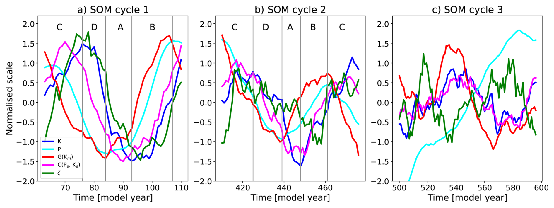
Figure 6 Energetics for three different SOM cycles in the SO30 region. Time series of volume integrated (90–30° S) available potential energy (P), total kinetic energy (K), energy conversion of eddy potential energy to eddy kinetic energy (C(P_e,K_e)), mean energy input by the wind (G(K_m)) and a measure of the non-zonality of the flow field ζ for (a) SOM cycle 1 (model year 63–114), (b) SOM cycle 2 (model year 324–378) and (c) SOM cycle 3 (model year 500–600). All time series represent 5 year running averages. Note that each quantity X is normalised according to $(X-X_{\text{mean}})/{\mathit{\sigma }}_{X\mathrm{1}}$, where σ_X1 is the standard deviation of the quantity in SOM cycle 1. The vertical lines divide the SOM cycle into the four regimes (A–D) according to Hogg and Blundell (2006), as described in Sect. 3.3. Note that SOM cycle 3 cannot easily be divided into these regimes.

The temporal evolution for SOM cycle 2 and 3 are shown in Fig. 6b and c, respectively. Note that we normalised the quantities as $(X-X_{\text{mean}})/{\mathit{\sigma }}_{X\mathrm{1}}$, where we use the standard deviation of the first cycle as reference. Equation (5) shows that the rate of change of K_e, and therefore K, is mainly influenced by C(P_e,K_e). Large transfers of potential to kinetic energy feed almost directly into the eddy kinetic energy field. Consistent with this, in all three SOM cycles, K and C(P_e,K_e) are positively correlated with a lag varying between 1–5 years. The non-zonality parameter ζ loses its multidecadal oscillatory behaviour in SOM cycle 3, in contrast to the pronounced variability found during SOM cycles 1 and 2 (Fig. 6a and b). During SOM cycle 1 and 2, the minima and maxima of P lead the minima and maxima of K with an approximate phase difference of 90°. The phase offset between P and K vanishes completely in SOM cycle 3 due to the altered behaviour of P as a consequence of stratification changes in the water column. Furthermore, a clear phase difference between G(K_m) and C(P_e,K_e) is found in SOM cycle 1, which is essential to sustain the SOM (Hogg and Blundell, 2006; Le Bars et al., 2016; Jüling et al., 2018). In SOM cycle 3, however, G(K_m) and C(P_e,K_e) begin to co-vary, with reduced phase differences between their minima and maxima.

Figure 6 shows the energetics integrated over the entire Southern Ocean. Performing the same analysis for the Atlantic sector alone yields a similar behaviour: during SOM cycles 1 and 2, the phase differences between the energy terms resemble those found in the SO30 region, while these phase relationships disappear during SOM cycle 3 (Fig. A7). In contrast, in the Pacific sector the emergence of the SOM-P cycle is not accompanied by clear phase differences during SOM cycle 3 that are consistent with the established framework of Hogg and Blundell (2006) (Fig. A8). This suggests that, unlike in the Atlantic sector, the SOM-P may not be strongly influenced by eddy–mean flow interactions. In conclusion, the reorganization of the Southern Ocean density field leads to a fundamental change in the mechanical energy budget, particularly affecting the phase relationships between P and K, and between G(K_m) and C(P_e,K_e). As these phase relationships are essential for sustaining the SOM, their alteration due to the AMOC collapse leads to the disappearance of the SOM cycle in the Atlantic sector.

3.4 Changes in Southern Ocean deep convection

Changes in stratification likely influence deep convection across the Southern Ocean and the exact role of deep convection in the SOM variability is not completely clear (Jüling et al., 2018). The reason is that convection is parameterised (using the KPP mixing scheme in POP), which provides enhanced mixing without explicitly resolving vertical velocities. Hence, the contribution by deep convection cannot be assessed using the mechanical energy pathways (Jüling et al., 2018). A recent study by Ford et al. (2026), based on the analysis of a high-resolution CESM simulation, found only weak evidence for atmosphere–ocean feedbacks contributing to Southern Ocean multidecadal variability and instead attributed this variability primarily to oceanic processes. They propose that the SOM mechanism operates as part of a coupled oscillator involving Southern Ocean deep convection events, with salinity upwelling east of Maud Rise playing a crucial role. These findings support the conclusion of Jüling et al. (2018) that deep convection can also play a substantial role in sustaining the SOM.

Based on the largest differences in the maximum and variance of the mixed layer depth (MLD) between model years 500–600 and 1–100 (Fig. 7a and b), four regions are identified for further analysis. Similar to Jüling et al. (2018), we define the Weddell Gyre to Kerguelen Plateau (WGKP) region as 80–50° S and 35° W–80° E (green outlined region in Fig. 7b). The brown-outlined region in the eastern Indian sector south of Australia, extending from 70–50° S and from 80–150° E, is hereafter referred to as AU. The convective region highlighted in magenta, located at longitudes aligned with New Zealand and spanning 70–62° S and 160° E–170° W, is hereafter denoted as NZ. Finally, the blue-outlined western Pacific region, extending from 70–50° S and 110–60° W, is hereafter referred to as PA.

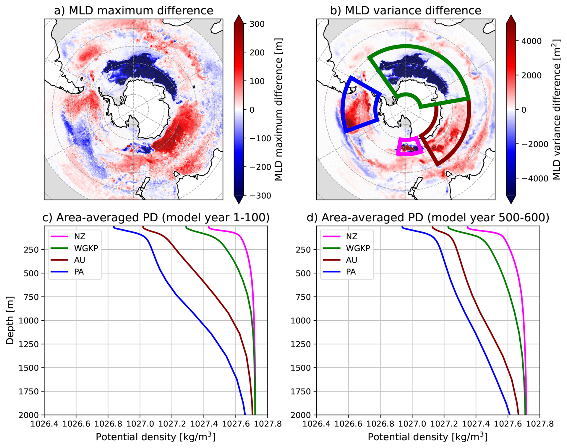
Figure 7 Mixed layer depth (MLD) and potential density (PD) properties in the SO30 region. Difference in the MLD between model year 500–600 and model year 1–100 of the (a) MLD maximum, and (b) variance in the SO30 region. The outlined regions denote the WGKP (green), the AU (brown), the NZ (magenta), and the PA (blue) region. (c, d): The area-averaged PD profiles in the four convective regions time-averaged over (c) model year 1–100, and (d) model year 500–600.

The area-averaged potential density (PD) profiles of the four regions are shown in Fig. 7c and d for model year 1–100 and model year 500–600, respectively. The stratification over the upper 2000 m is relatively weak for the NZ and WGKP regions, whereas the AU and PA regions are stronger stratified (Fig. 7c). Following the AMOC collapse, stratification increases in the NZ and WGKP regions, while the opposite is true for the AU and PA regions (Fig. 7d). A stronger (weaker) stratification reduces (increases) the MLD, which is found for the NZ and WGKP (AU and PA) regions.

To make the latter more explicit, we present the maximum MLD and Brunt-Väisälä frequency differences (relative to the first 100 model years) over the four regions in Fig. 8. The stratification in the WGKP region strongly increases in the upper 100 m, decreases in the layer just below (down to 250–500 m), and increases again at depths down to 2000 m (Fig. 8b). The NZ region exhibits an overall increase in stratification, with the strongest anomalies occurring in the upper 100 m. In contrast, the AU and PA regions show an overall decrease in stratification in the upper 1000–1500 m, and an increase at greater depths.

The stratification changes in the convective regions are related to a salinity-dominated reorganization of the water-column structure following the AMOC collapse (Fig. A9). The increased stratification in the deeper layers of the AU and PA regions, and in the intermediate layers of the NZ and WGKP regions, can be linked to a reduced poleward advection of warm and saline Circumpolar Deep Water (CDW) after the AMOC has weakened. Furthermore, a downward displacement or reorganization of Antarctic Intermediate Water (AAIW), identified by its salinity minimum, leads to reduced vertical salinity gradients causing weakening of the stratification. This mechanism explains the reduced stratification in the upper ∼1500 m of the AU and PA regions, and the weakening of stratification in the WGKP region between roughly 100 and 250–500 m. Although the reduced stratification barely penetrates into the WGKP region (Fig. A9), it dominates over the otherwise increasing stratification in the same depth range. The stratification changes north of the NZ convective region show a similar structure to those in the WGKP region.

Although the stratification weakening over the AU and PA regions induces a slightly deeper mixed-layer (Fig. 8c and d), the stratification remains sufficiently strong such that the MLD responses are limited. A weak multidecadal oscillation arises after the collapse of the AMOC with comparable periods to that of the SOM-P index (Fig. A10c and d). In contrast, the stratification over the NZ region remains relatively weak compared to the other three regions (Fig. 7c and d), making this region the most prone to the deepest MLD events after the AMOC collapse. The onset of deep convection with strong multidecadal variability (Fig. A10a) in this region is closely linked to the stratification anomalies in the upper 100 m after the AMOC collapse (Figs. 7a).

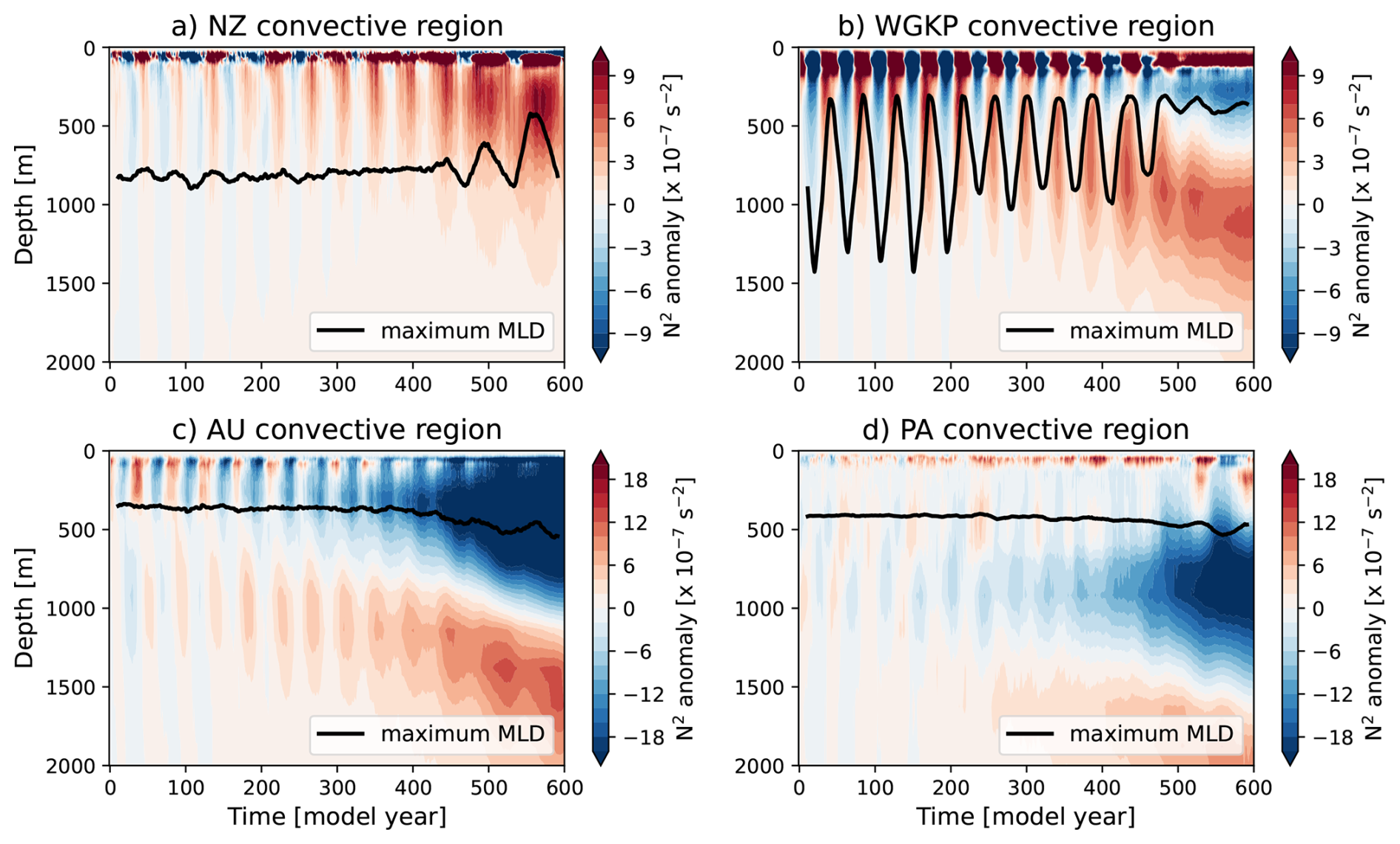
Figure 8 Maximum MLD (black line) and area-averaged N² anomalies (with respect to mean N² over the first 100 model years) in the (a) NZ, (b) WGKP, (c) AU, and (d) PA convective regions.

Up to the AMOC collapse, strong MLD changes occur in the WGKP region with a period closely following that of the SOM index (Fig. A10b). Over these 400 years, the MLD in the NZ region is deep (∼800 m) but its variability is relatively small (Fig. A10a). Deep convection events in the WGKP convective region follow a convection–restratification mechanism (Jüling et al., 2018; Dijkstra and van der Heydt, 2017; Latif et al., 2013). Heat originating from the inflow of relatively warm North Atlantic Deep Water (NADW) is transported into the Weddell Sea by the westward return flow in the southern branch of the Weddell Gyre, where it remains effectively trapped within the gyre circulation. The accumulation of heat at mid-depth levels destabilizes the water column and can eventually trigger deep convection. Once the mid-depth heat reservoir is depleted, convection shuts down (Fig. 8b). The multidecadal recharge of this heat reservoir depends on both the AMOC and the Weddell Gyre circulation (Jüling et al., 2018), and is closely related to the SOM variability as generated by the eddy-mean flow interaction mechanism described in the previous section. The ACC is modulated by these convective episodes, with the meridional pressure gradient weakening during non-convective phases due to gradual mid-depth warming of waters south of the ACC, and strengthening during convective phases as these waters cool. This variability in the pressure gradient leads to a corresponding weakening or strengthening of the ACC, typically with a lag of a few years (Fig. A11).

The stratification over the WGKP region is relatively weak compared to the AU and PA regions (Fig. 7), but increases due to the reduced inflow of NADW. As a result, the water column cannot support any deep convection (>1000 m) events anymore after the AMOC collapse. At the same time, stratification anomalies in the upper 100 m start to appear again over the NZ region, predominantly salinity-driven (not shown), and are apparently sufficient to initiate convection and support relatively strong MLD changes (Fig. 8a), which in turn affect the Drake Passage transport. After deep convection ceases in the WGKP region and the SOM cycle vanishes, a pronounced oscillatory signal still persists in the Drake Passage transport with a period similar to that of the SOM-P index (Fig. A1). Deep convection in the NZ region now leads the multidecadal oscillations in the Drake Passage transport (Fig. A11).

The occurrence of deep convection events have been linked to an overall strengthening of the ACC, as they facilitate the conversion of potential to kinetic energy, thereby energizing the ocean circulation (Xing et al., 2023). Indeed, we find an overall decrease in mean strength of the ACC (Fig. 1c), consistent with a decrease in C(P_e,K_e) (Fig. 4d) and the termination of deep convection events in the WGKP region.

This shift in Southern Ocean deep convection from the Atlantic to the Pacific sector is closely linked to the behaviour of the SOM-P index, which starts to exhibit pronounced multidecadal variability around the same time deep convection in the NZ region starts (Fig. 9b). The convective episodes in the NZ region now lead the oscillations in the SOM-P index, in a similar way the minima and maxima of the WGKP convective episodes led the minima and maxima of the SOM-index (Fig. 9a). Whereas the SOM mechanism involves a combination of eddy–mean flow interactions and deep convection in the WGKP region, the oscillations emerging after the AMOC collapse cannot be explained by the first mechanism, as its signature is not detectable in the mechanical energy budget over the SO30 region. Instead, the SOM-P variability has a purely convective origin and in this way, the Pacific sector becomes the primary source region for multidecadal variability of the Southern Ocean origin when the AMOC has collapsed.

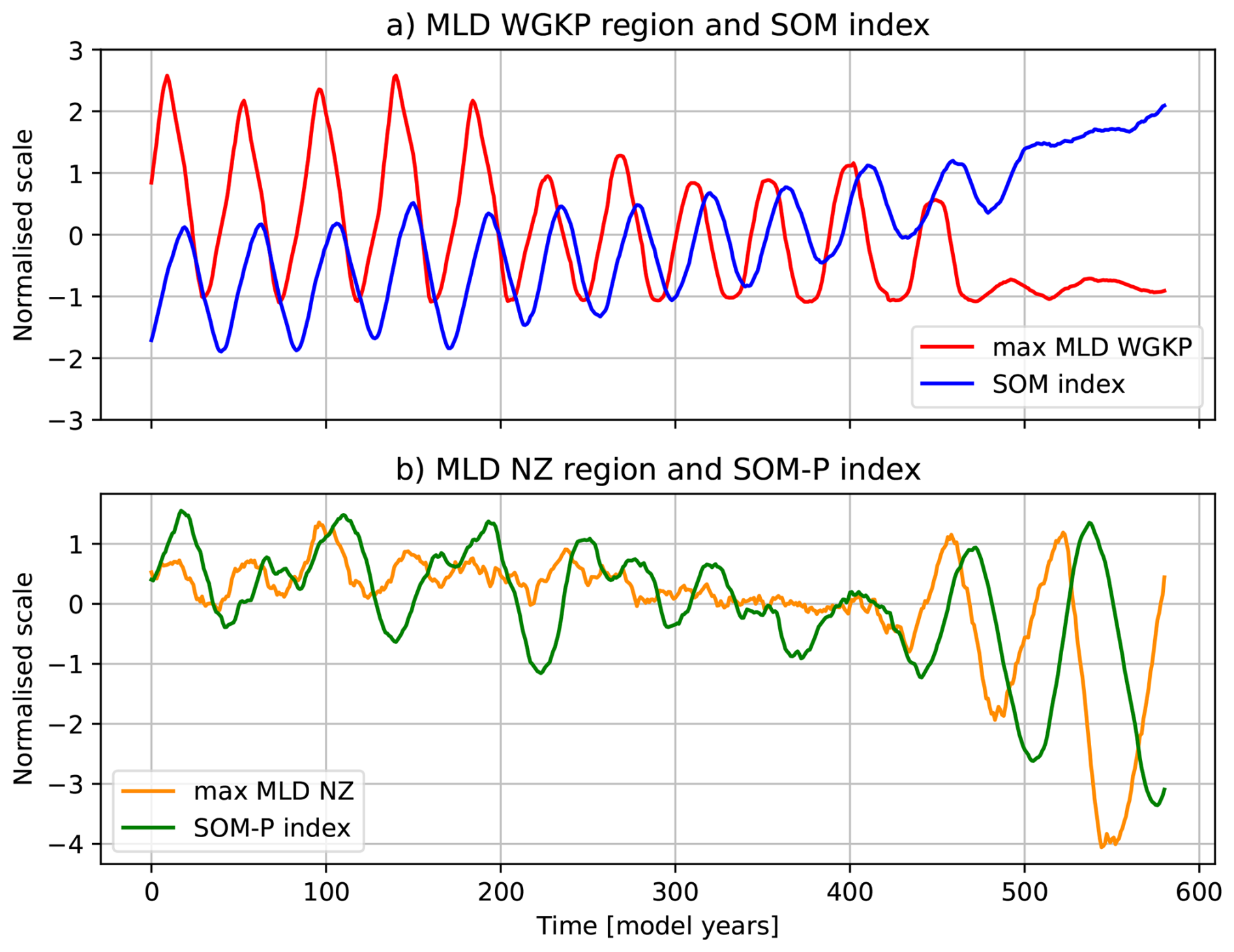
Figure 9 (a): SOM-index (blue), and the maximum MLD in the WGKP region (red). (b): SOM-P index (green), and the maximum MLD in the NZ region (orange). Note that all time series are normalised and mean-centered, and a moving average of 20 years has been applied.

4 Conclusions

In the strongly-eddying POP model, multidecadal intrinsic variability appears which is not found in the non-eddying version of the same model (Le Bars et al., 2016; Jüling et al., 2018; van Westen et al., 2025). The same variability, referred to as the Southern Ocean Mode (SOM), occurs in the Community Earth System Model version with a strongly eddying ocean component (van Westen and Dijkstra, 2017; Chang et al., 2020; Wang et al., 2022; Ford et al., 2026). It is important to understand the mechanisms of this intrinsic variability in more detail, in addition to other mechanisms which have been suggested, as it is potentially relevant to interpret observed multidecadal Antarctic sea-ice variability (Morioka et al., 2024).

In this study, we use the same strongly-eddying POP version as in Le Bars et al. (2016) to study the effect of the AMOC on the SOM. Previous studies have shown that the SOM introduces multidecadal variability (of a few Sv) in the AMOC strength at 26° N caused by northward Rossby wave propagation in the Atlantic Ocean (van Westen and Dijkstra, 2017). We demonstrated here that the SOM owes its existence to the density field in the Southern Ocean which is affected by the AMOC. A strong weakening of the AMOC induces substantial changes in the Southern Ocean density structure, leading to the disappearance of the SOM in the Atlantic sector and the emergence of the SOM-P in the Pacific sector. Although a complete understanding of the underlying mechanisms and pathways would require detailed heat- and freshwater budget analyses, our results show consistent salinity-driven stratification changes associated with a reduced poleward advection of CDW and deepening or reorganization of AAIW.

An analysis of the terms in the mechanical energy balance shows that eddy-mean flow interactions weaken under a decreasing AMOC strength and that phase differences between the input of the wind (G(K_m)), and the baroclinic conversion term (C(P_e,K_e)) decrease. This disrupts the coupling between eddy generation by baroclinic instability, jet zonality, and wind input. Furthermore, a weakening of the AMOC increases the stratification in the WGKP region, mainly due to reduced upper layer salinities associated with a reduced inflow of NADW, thereby weakening the deep convection events in this region. The primary source of convection appears to shift to the Pacific sector, where deep convection events begin to emerge only after the AMOC has collapsed. These convective events in the Pacific now cause the oscillatory behaviour of the Drake Passage. Although not studied here, this is also expected to affect variability in the Weddell and Ross Gyre circulations (Jüling et al., 2018).

The horizontal and vertical density structure of the Southern Ocean is thus modified in a way that weakens eddy–mean flow interactions and shifts the primary source of deep convection, leading to the disappearance of the SOM. However, despite being very localized, convection in the Pacific sector remains sufficiently strong to sustain a mode of multidecadal variability, namely the SOM-P. Although the exact role of convection in driving multidecadal oscillations in the Southern Ocean remains uncertain, this study also underscores the importance of deep convection events in shaping Southern Ocean multidecadal variability in climate models (Ford et al., 2026).

While this study is based on an ocean-only model, atmospheric variability is likely to play a role. Although Ford et al. (2026) found only weak evidence for atmosphere–ocean feedbacks contributing to Southern Ocean multidecadal variability, multidecadal variability in Southern Ocean temperatures or sea-ice extent may influence large-scale climate modes such as the Interdecadal Pacific Oscillation (IPO) through atmospheric teleconnections (Chang et al., 2020). Conversely, atmospheric variability, including changes in sea level pressure patterns such as the Amundsen Sea Low (Dalaiden et al., 2024), may feed back onto the ocean circulation and variability. This highlights the importance of understanding intrinsic multidecadal variability in the Southern Ocean and its potential coupling to the atmosphere.

Although the SOM cannot be clearly identified in the historical record (Jüling et al., 2020), its presence in the CESM (van Westen and Dijkstra, 2020; Ford et al., 2026), and the consistency of its underlying mechanism with that of a mode of multidecadal variability identified in a quasi-geostrophic model (Hogg and Blundell, 2006) provide strong support that the SOM is a dynamically meaningful feature in the present-day ocean. The analysis here has clearly demonstrated a strong connection between the SOM and the AMOC, with pronounced changes in multidecadal variability, ocean density field, and deep convection following an AMOC collapse. These changes have significant implications for the mean state of the Southern Ocean, including a marked cooling near the base of the Antarctic ice shelf. This, in turn, affects Antarctic sea-ice variability and basal melt, suppresses deep convection in the Weddell Sea, and may affect teleconnections with other ocean basins.

Appendix A: Additional figures

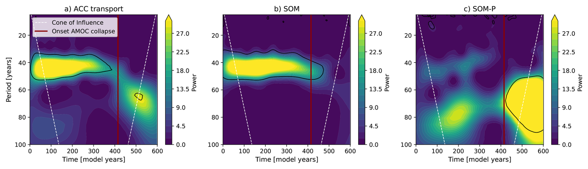
Figure A1 Wavelet (Morlet) power spectra for (a) the ACC transport, (b) the SOM index, and (c) the SOM-P index. Black contours indicate power significant at the 95 % level relative to an AR(1) red-noise background. The vertical red line marks the onset of the AMOC collapse, and the white dashed lines indicate the cone of influence.

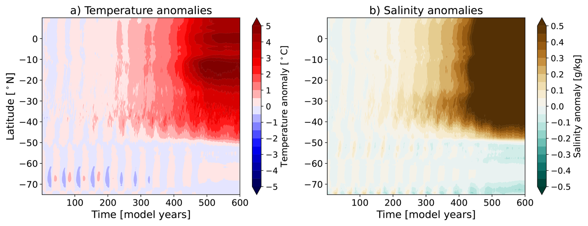
Figure A2 Hövmoller diagram of depth- and zonally-averaged (300–700 m, 55–5° W) (a) temperature and (b) salinity anomalies with respect to the first 100 model years.

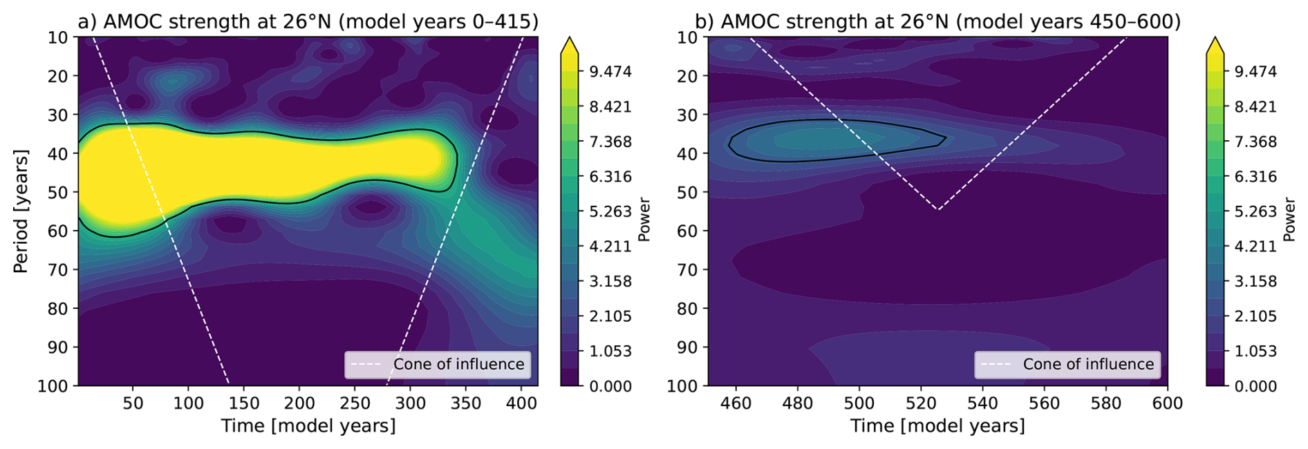
Figure A3 Wavelet (Morlet) power spectra for the quadratically detrended AMOC strength from (a) model year 0–415, and for (b) model year 450–600. Black contours indicate power significant at the 95 % level relative to an AR(1) red-noise background, and the white dashed lines indicate the cone of influence.

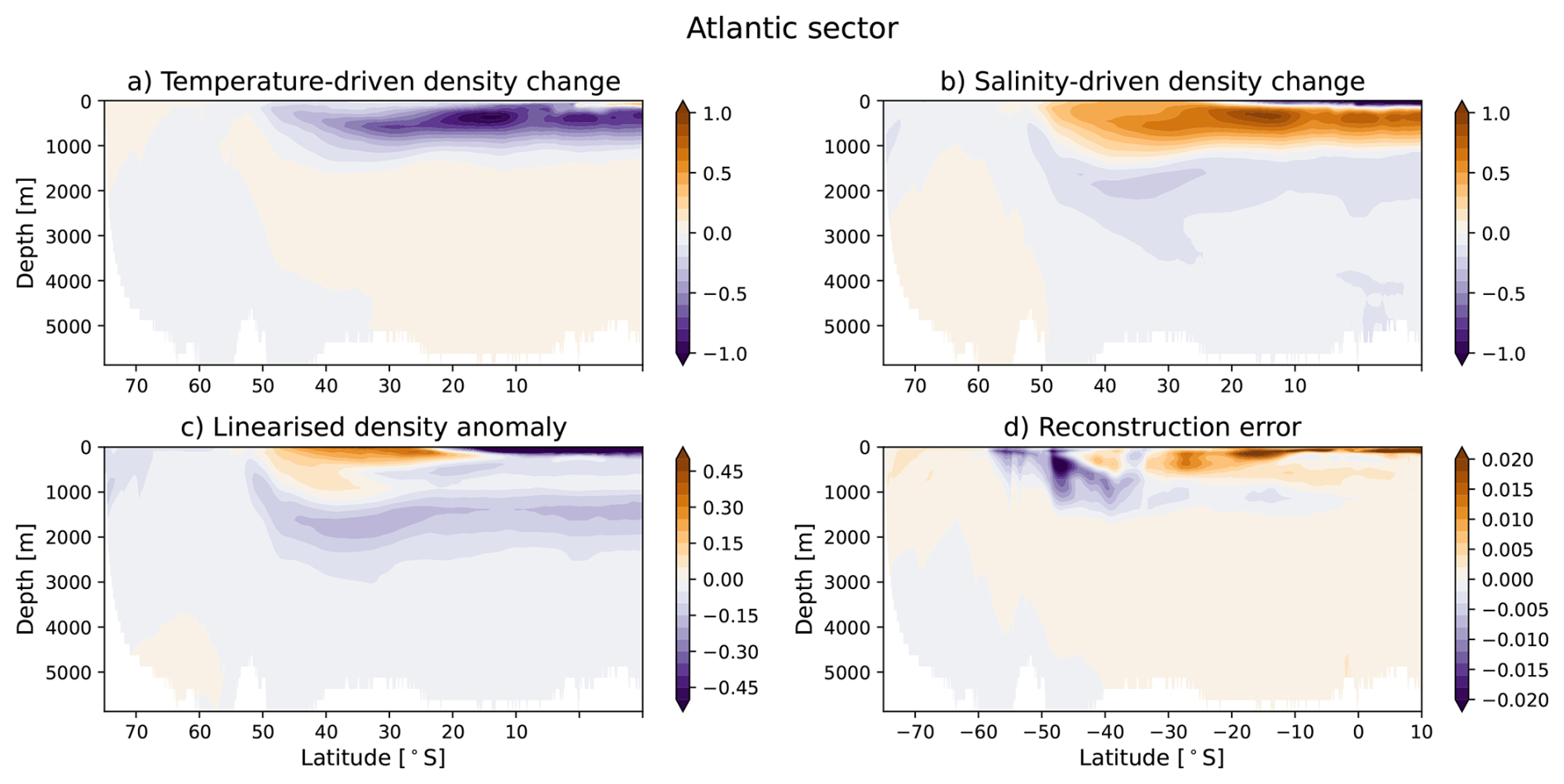
Figure A4 Linear density decomposition in the Atlantic sector. Zonal-averaged (60° W–25° E) (a) temperature-driven and (b) salinity-driven density changes (model year (500–600) minus model year (1–100)). (c) Linearised density anomaly, obtained as the sum of the temperature- and salinity-driven contributions. (d): Reconstruction error of the linearised density anomaly relative to the actual density anomaly.

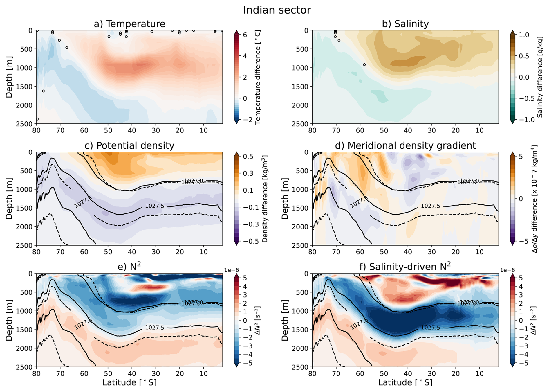
Figure A5 Temperature, salinity, meridional density gradient and zonal velocity differences in the Indian sector. Zonal-averaged (25–150° E) (a) temperature, (b) salinity, (c) meridional density gradient and (d) zonal velocity differences in the upper 2500 m before and after the AMOC collapse (model year (500–600) minus model year (1–100)). In (c), the solid (dashed) black lines denote isopycnals of model year 1–100 (500–600). Plotted isopycnals are referenced to 5° N and the displayed (from top to bottom) ones are: 1025.1 (1025.2), 1026.5 (1026.9), and 1027.6 (1027.5) kg m⁻³ for model year 1–100 (500–600). In (d), the vertical dashed lines denote the mean ACC latitude band for model year 1–100.

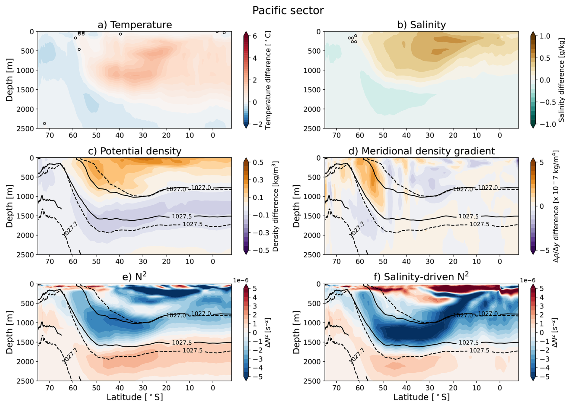
Figure A6 Temperature, salinity, meridional density gradient and zonal velocity differences in the Pacific sector. Zonal-averaged (150° E–60° W) (a) temperature, (b) salinity, (c) meridional density gradient and (d) zonal velocity differences in the upper 2500 m before and after the AMOC collapse (model year (500–600) minus model year (1–100)). In (c), the solid (dashed) black lines denote isopycnals of model year 1–100 (500–600). Plotted isopycnals are referenced to 5° N and the displayed (from top to bottom) ones are: 1025.6 (1025.6), 1027.0 (1026.9), and 1027.6 (1027.6) kg m⁻³ for model year 1–100 (500–600). In (d), the vertical dashed lines denote the mean ACC latitude band for model year 1–100.

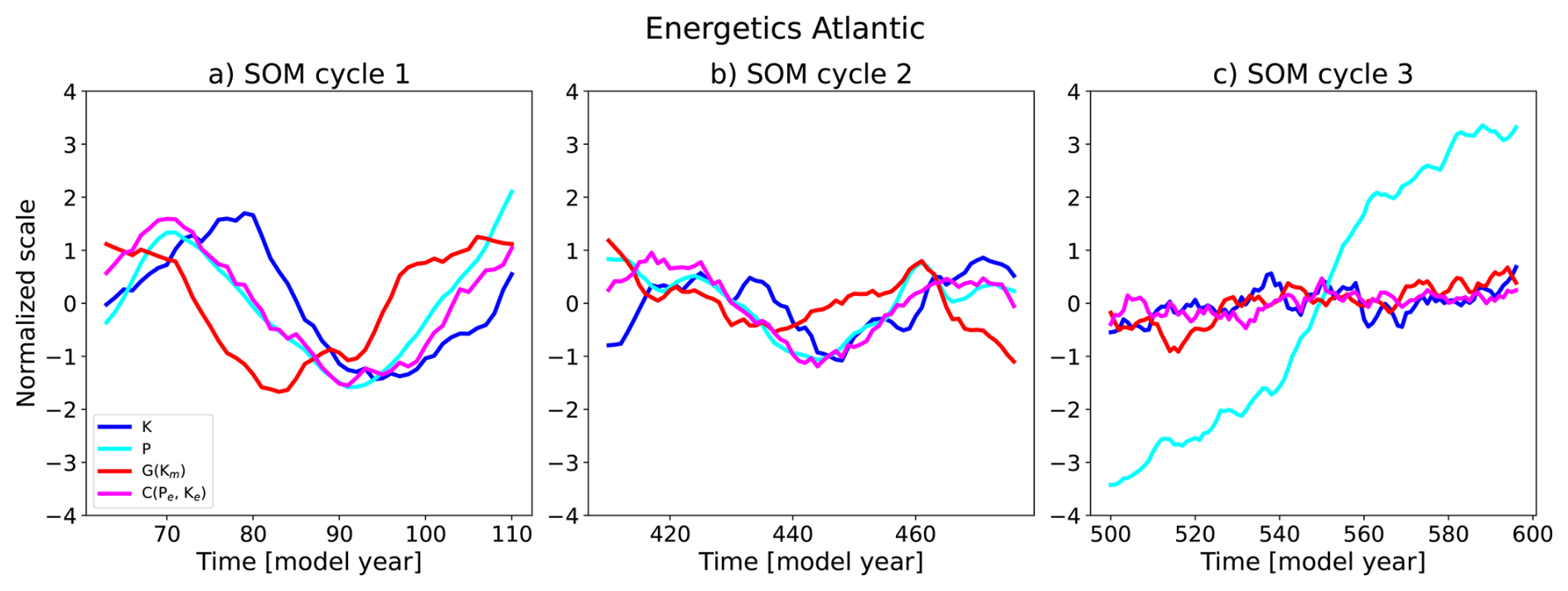
Figure A7 Energetics for three different SOM cycles in the Atlantic sector. Similar to Fig. 6, but now for the Atlantic sector (90–30° S, 60° W–25° E).

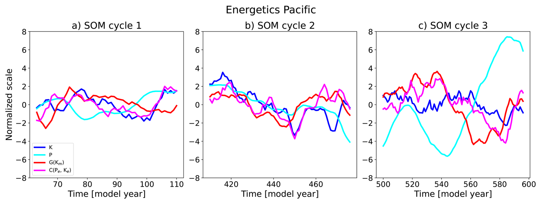
Figure A8 Energetics for three different SOM cycles in the Pacific sector. Similar to Fig. 6, but now for the Pacific sector (90–30° S, 150° E–60° W).

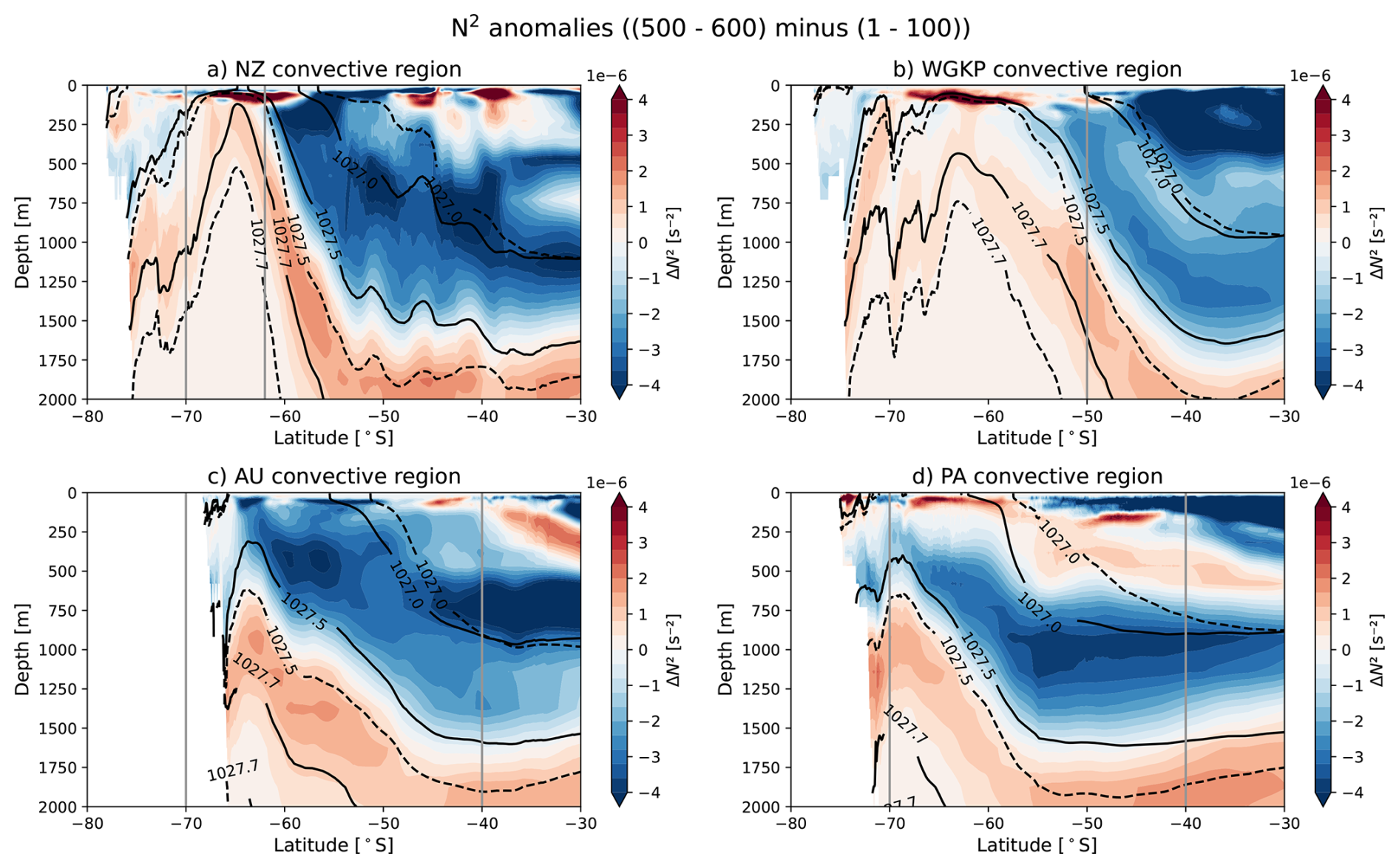
Figure A9 Zonally averaged N² anomalies in SO30 convective regions. (a) Zonally averaged (150–170° E) N² in the NZ convective region (model year (500–600) minus (1–100)). (b) Same as (a), but now zonally averaged over the WGKP convective region (35–80° W), (c) for the AU convective region (80–150° E), and (d) for the PA convective region (110–160° W). The solid (dashed) black lines denote zonally averaged isopycnals of model year 1–100 (500–600). Plotted isopycnals are (from top to bottom): 1027.0, 1027.5, and 1027.7 kg m⁻³. The grey vertical lines denote the meridional boundaries of the respective convective regions.

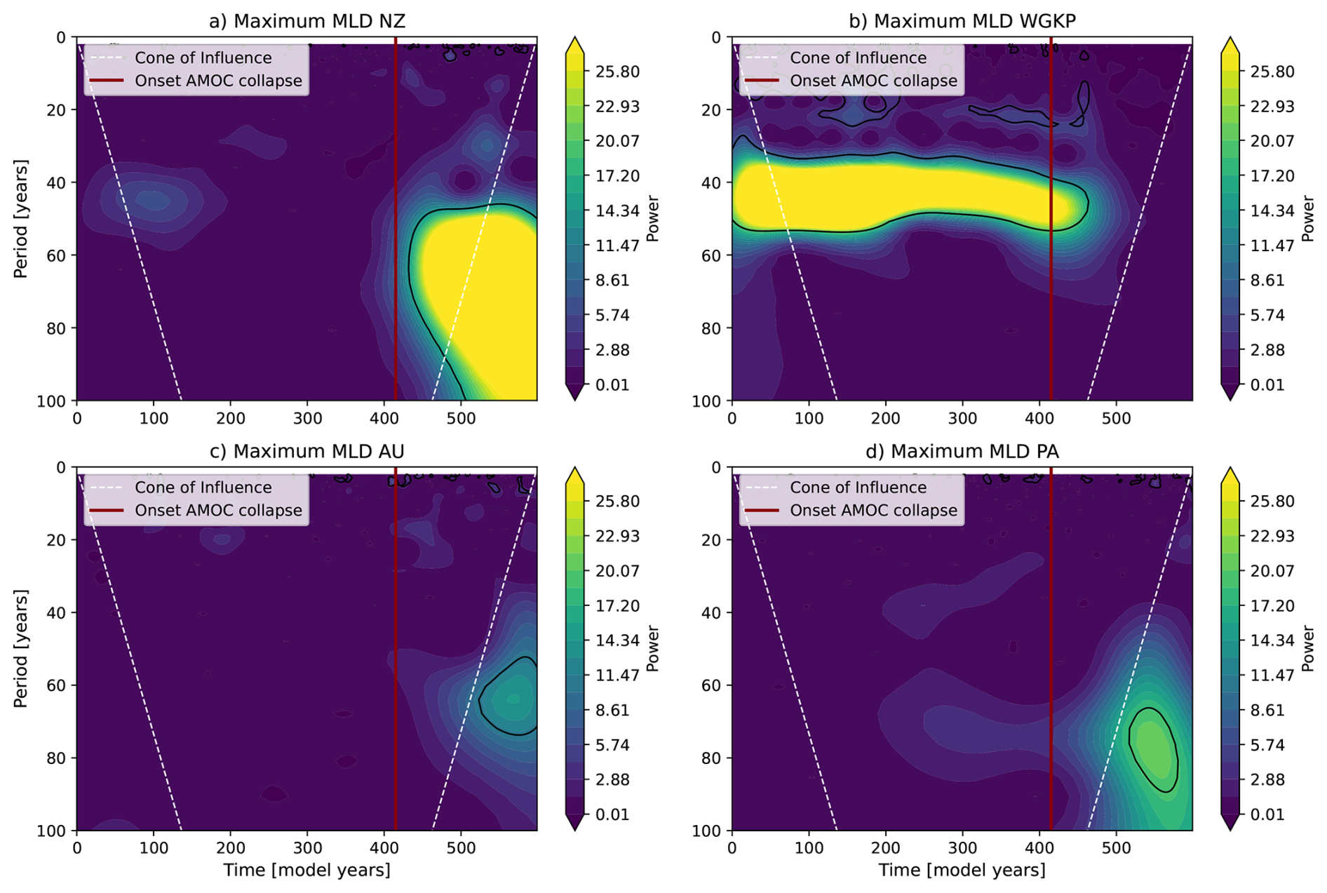
Figure A10 Wavelet (Morlet) power spectra for the maximum MLD in (a) the NZ convective region, (b) the WGKP convective region, (c) the AU convective region, and (d) the PA convective region. Black contours indicate power significant at the 95 % level relative to an AR(1) red-noise background. The vertical red line marks the onset of the AMOC collapse, and the white dashed lines indicate the cone of influence.

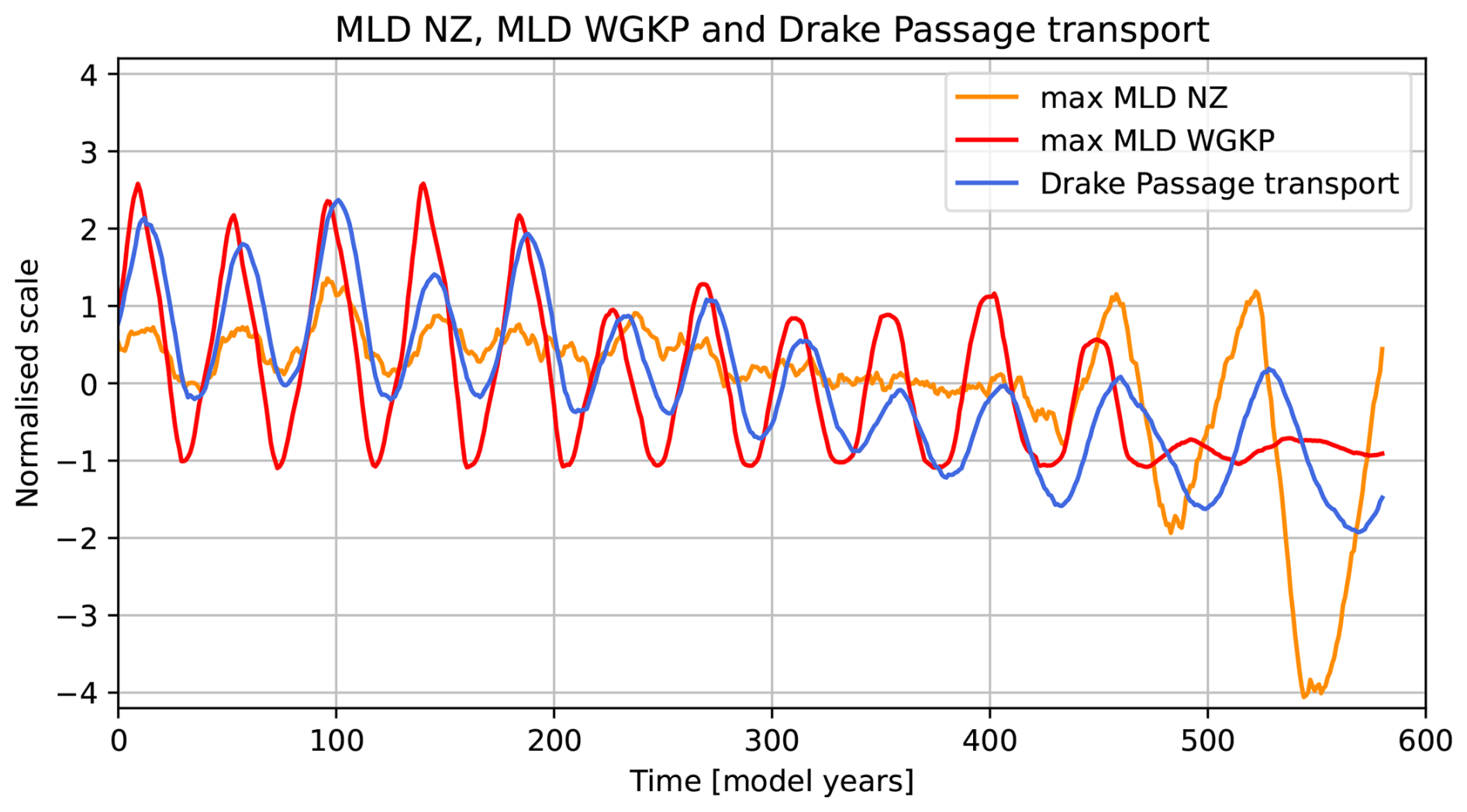
Figure A11 Drake Passage transport (blue), and the maximum MLD in the WGKP region (red) and NZ region (orange). A moving average of 20 years has been applied to all time series.