Dynamic and steric sea-level changes due to a collapsing AMOC in the Community Earth System Model

A collapse of the Atlantic Meridional Overturning Circulation (AMOC) leads to a redistribution of dynamic sea level (DSL) across the global ocean surface. Here, we investigate DSL and steric sea-level responses under different AMOC strengths using the Community Earth System Model and two stand-alone ocean configurations (strongly eddying and parameterising eddy effects) with the Parallel Ocean Program. For our analysis, we employ various quasi-equilibrium freshwater hosing experiments in which AMOC collapses were reported. As the AMOC begins to collapse, the DSL substantially rises over the Atlantic Ocean and Arctic Ocean. Regions outside the Atlantic basin display a relatively small DSL drop. The largest DSL trends are found over the North Atlantic Ocean and reach +6 mm yr⁻¹ over a 100-year period, with DSL trends near densely-populated coastal regions of up to +4 mm yr⁻¹. This is a considerable contribution to local sea-level rise compared to the observed global mean sea-level rise of +3.3 mm yr⁻¹. DSL trends obtained from the quasi-equilibrium experiments include a contribution from the freshwater hosing itself (≈ +0.2 mm yr⁻¹), which is typically a factor 10–20 smaller than DSL response during the AMOC collapse. Moreover, a collapsed AMOC increases the net oceanic heat uptake leading to more than 50 cm of global mean thermosteric sea-level rise on millennial timescales (> 2000 years). These results highlight the potential value of accounting for an AMOC collapse scenario when developing or applying sea-level rise projections for the North Atlantic Ocean.

1 Introduction

A collapse of the Atlantic Meridional Overturning Circulation (AMOC) modifies the planetary heat and salinity redistribution and this causes large-scale climate shifts (Orihuela-Pinto et al., 2022). For example, the Northern Hemisphere cools and receives less precipitation under a reduced AMOC strength (Liu et al., 2020; Bellomo et al., 2023; Bellomo and Mehling, 2024; van Westen et al., 2024b). Certain regions, such as Europe, are expected to see drastic changes in their present-day climate. The European climate would experience more intense winter storms and cold extremes, and more droughts (Vellinga and Wood, 2002; Jacob et al., 2005; Brayshaw et al., 2009; Jackson et al., 2015; Meccia et al., 2024; van Westen and Baatsen, 2025; van Westen et al., 2025b).

Apart from atmospheric impacts, the AMOC also modulates dynamic sea level (DSL) (Bryan, 1996; Levermann et al., 2005). DSL is the height of the sea surface above the geoid and has a global mean of zero (Gregory et al., 2019). DSL is primarily determined by ocean circulation and ocean density, both of which are influenced by different AMOC strengths (Vanderborght et al., 2025). The AMOC strength is expected to significantly decline by 18 %–45 % under 21st century climate change (Weijer et al., 2020; Bonan et al., 2025). This AMOC weakening causes DSL rise over the North Atlantic Ocean (≥40° N) and the Arctic Ocean (Landerer et al., 2007; Katsman et al., 2008; Yin et al., 2009; Chen et al., 2019; Lyu et al., 2020), with local DSL trends exceeding +4 mm yr⁻¹ under a high-emission scenario (Ferrero et al., 2021; Pardaens, 2023). Evidence of AMOC variability has already been detected in sea-level observations from both satellite altimetry and tide gauges along North Atlantic coasts (Bingham and Hughes, 2009; Little et al., 2019). This is important because it indicates that AMOC fluctuations can influence flood risk, which is projected to increase under AMOC weakening (Volkov et al., 2023; Howard et al., 2024).

A fully-collapsed AMOC could lead to even larger DSL rise than under AMOC weakening alone, with regional DSL rise up to +1 m (Levermann et al., 2005; van Westen et al., 2024b, 2025a). However, the latest generation of coupled climate models only project significant AMOC weakening and an AMOC collapse event before 2100 is assessed as unlikely (Weijer et al., 2020; Fox-Kemper et al., 2021; Bonan et al., 2025; Baker et al., 2025). There are indications that most climate models have a too stable AMOC and likely underestimate the risk of an AMOC tipping event under climate change (Liu et al., 2017; van Westen and Dijkstra, 2024; Vanderborght et al., 2025). If the AMOC would start to collapse this century (Ditlevsen and Ditlevsen, 2023; van Westen et al., 2025d; Drijfhout et al., 2025), the AMOC strength would reduce faster than in the latest Intergovernmental Panel for Climate Change (IPCC) assessment (Fox-Kemper et al., 2021). This means that DSLs over the North Atlantic Ocean and Arctic Ocean would increase faster than is currently anticipated for. This information on accelerated DSL rise is crucial for North Atlantic coastal communities and for developing adaptation strategies to sea-level rise (Haasnoot et al., 2018; Biesbroek et al., 2025).

DSL projections are sensitive to the climate model mean state, model biases, and wind and buoyancy forcing (Lyu et al., 2020; Jesse et al., 2024). This complicates efforts to disentangle the individual contributions of 21st century AMOC weakening and climate change to DSL projections. The AMOC contribution to DSL changes can now be isolated using recent simulations performed with the Community Earth System Model (CESM, version 1.0.5), in which a slowly increasing freshwater flux forcing (i.e., hosing) causes an AMOC collapse (van Westen et al., 2024b). The AMOC tipping event is driven by intrinsic climate feedbacks, allowing DSL changes associated solely with the AMOC collapse to be isolated. Global mean steric sea-level changes caused by a collapsing AMOC can also be studied using the CESM. Inspired by the work of Levermann et al. (2005), here we aim to revisit DSL changes in a modern complex climate model under a collapsing AMOC.

The structure of this study is as follows. Section 2 introduces the CESM configuration, together with a description of the two stand-alone ocean simulations used. In Sect. 3, we present DSL changes under a collapsing AMOC and consider DSL changes for different AMOC mean states. Steric sea-level variations are examined in Sect. 4. Finally, Sect. 5 summarises and discusses the main findings.

2 Methods

2.1 Fully-coupled climate model simulations

For our analysis we will make use of the fully-coupled CESM as in van Westen et al. (2024b). The used CESM configuration has horizontal resolutions of 1°×1° for the ocean/sea ice and 2°×2° for the atmosphere/land components, respectively. The ocean component is the Parallel Ocean Program version 2 (POP2, Smith et al., 2010), the sea-ice component is the Community Ice Code version 4 (CICE4, Hunke and Lipscomb, 2008), the atmospheric component is the Community Atmosphere Model version 4 (CAM4, finite volume configuration, Neale et al., 2013), and the land component is the Community Land Model version 4 (CLM4, Lawrence et al., 2011). The CESM has prescribed ice sheets. Note that the horizontal ocean resolution of 1°×1° is too coarse to explicitly resolve mesoscale processes (Hallberg, 2013), such as ocean eddies, and their processes are parameterised (Gent and Mcwilliams, 1990). Hence, we refer to this CESM version as the low-resolution CESM (LR-CESM). We present an analysis of different LR-CESM simulations, with a summary provided in Table 1. Further details of the different model experiments are given below.

Table 1 Overview of the different simulations, which includes: simulation name, experiment, freshwater flux forcing (varying or fixed), duration, and horizontal resolutions for the oceanic and atmospheric components.

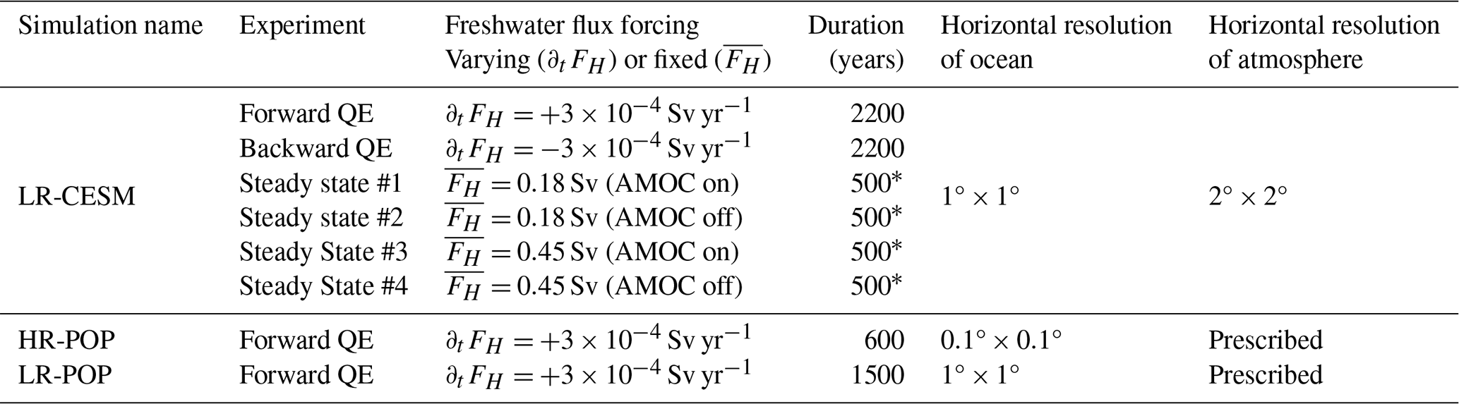
^* Only the last 50 model years are analysed.

The LR-CESM has constant pre-industrial greenhouse gas concentrations and was forced under an increasing surface freshwater flux forcing, F_H, which was applied over the 20 to 50° N latitude band in the Atlantic Ocean. This freshwater flux forcing was compensated over the remaining parts of the ocean surface to conserve the total ocean salinity. The F_H was increased at a slow rate of $\mathrm{3}\times {\mathrm{10}}^{-\mathrm{4}}$ Sv yr⁻¹, reaching a maximum value of F_H=0.66 Sv (model year 2200). The slow forcing rate ensures that the AMOC remains close to its equilibrium for that particular F_H (van Westen et al., 2024a, 2025c) and that transitions are caused by internal (ocean) dynamics, a so-called quasi-equilibrium (QE) hosing simulation. The AMOC reaches its tipping point in model year 1758 (F_H=0.527 Sv, van Westen et al., 2024b) and takes about 100 years to collapse, the AMOC strength time series is shown in Fig. 1a (black curve). More details on AMOC properties, AMOC tipping time estimate, and AMOC collapse climate impacts in the CESM were presented in previous work (van Westen et al., 2024b, a; van Westen and Baatsen, 2025; van Westen et al., 2025b, d).

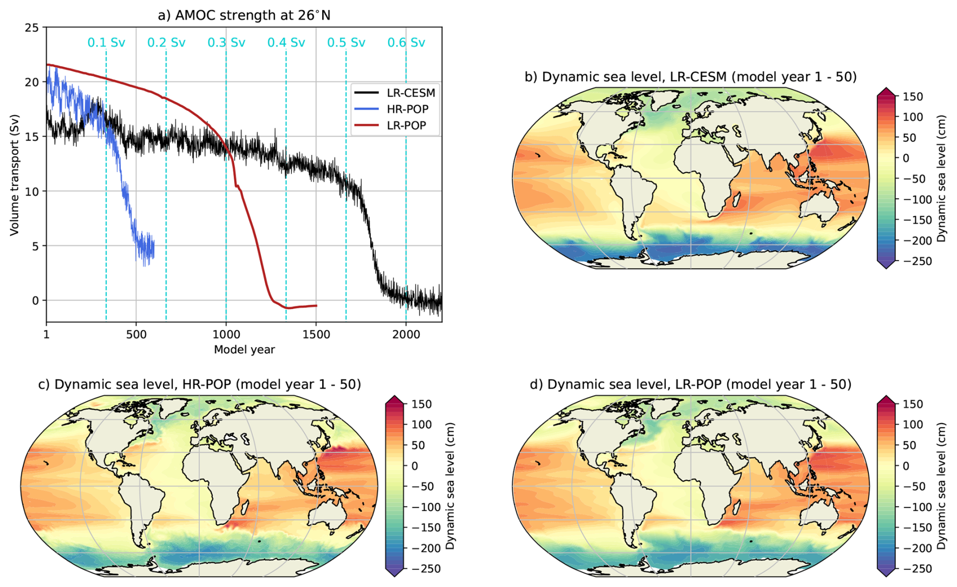
Figure 1 (a) The AMOC strength at 1000 m and 26° N for the quasi-equilibrium LR-CESM, HR-POP and LR-POP. (b–d) The time-mean DSL (first 50 model years) for the LR-CESM, HR-POP and LR-POP.

One side effect of the hosing approach is that DSL is directly influenced by variations in the freshwater flux forcing through density changes. This F_H contribution on DSL is small for short time intervals, and internal dynamics such as an AMOC collapse (100 years, ΔF_H=0.03 Sv) then dominate DSL responses. However, over the full QE hosing simulation (2200 years, ΔF_H=0.66 Sv) this contribution needs to be considered and will be quantified by analysing the accompanying backward simulation that was performed. Starting in model year 2200 (F_H=0.66 Sv) of the LR-CESM, the F_H was decreased at the same rate of $\mathrm{3}\times {\mathrm{10}}^{-\mathrm{4}}$ Sv yr⁻¹, resulting in a 4400-year long QE hysteresis simulation (see also Fig. 5a). The AMOC starts to recover from model year 4091 (F_H=0.093 Sv), which is at a much lower F_H than the collapse and clearly demonstrating AMOC hysteresis behaviour under varying F_H (van Westen and Dijkstra, 2023).

The F_H contribution to DSL is identical for a given F_H within the multi-stable regime, and differences in DSL are therefore attributed to different AMOC regimes. The QE hosing simulation is mostly in a weak transient state and to obtain a climate state (almost) free of transient effects we analyse the statistical equilibria for fixed F_H, indicated by $\stackrel{\mathrm{‾}}{F_H}$. These equilibria have time-invariant statistics and their radiative imbalance at top of atmosphere is almost zero (van Westen and Baatsen, 2025), meaning that natural climate variability is dominant. Four statistical equilibria were obtained by branching simulations from the QE LR-CESM within the multi-stable regime and fixed F_H, these simulations were integrated for 500 years during which the AMOC equilibrates (van Westen et al., 2024a), the last 50 model years are considered for the analyses. The statistical equilibria were obtained for the “AMOC on” regime at $\stackrel{\mathrm{‾}}{F_H}=\mathrm{0.18}$ Sv (model year 600) and $\stackrel{\mathrm{‾}}{F_H}=\mathrm{0.45}$ Sv (model year 1500), and similarly for the “AMOC off” regime at $\stackrel{\mathrm{‾}}{F_H}=\mathrm{0.18}$ Sv (model year 3800) and $\stackrel{\mathrm{‾}}{F_H}=\mathrm{0.45}$ Sv (model year 2900). The hosing-corrected DSL changes that arise from different AMOC regimes can then be determined by comparing “AMOC off” to “AMOC on” for both $\stackrel{\mathrm{‾}}{F_H}=\mathrm{0.18}$ Sv and $\stackrel{\mathrm{‾}}{F_H}=\mathrm{0.45}$ Sv. Due to computational constraints, only single realisations are available for the QE hysteresis simulation and for the four statistical equilibria.

2.2 Ocean-only simulations

As noted for the LR-CESM, the effects of mesoscale processes on DSL are parameterised, and explicitly resolving them may lead to different DSL responses (van Westen and Dijkstra, 2021). This contribution can be assessed using a QE hosing simulation with a high-resolution (0.1°×0.1°) and strongly-eddying stand-alone POP simulation (van Westen et al., 2025a).

The POP has a prescribed atmospheric state that is seasonally repeating, consisting of near-surface atmospheric temperatures, bulk formula, river run-off fields and precipitation (Weijer et al., 2012; Toom et al., 2014). This atmospheric state is derived from the Coordinated Ocean Reference Experiment (CORE) forcing dataset (van Westen et al., 2025a). To be more specific, this means that POP dynamically resolves sea surface temperatures and the associated outgoing surface heat fluxes and outgoing freshwater fluxes (i.e., online computation), whereas these surface quantities are being “forced” towards their prescribed atmospheric state. The wind stress, river run-off and precipitation are not resolved by the POP and hence are seasonally repeating throughout the entire simulation (i.e., offline computation). The −1.8 °C isoline of the sea surface temperature climatology was used to prescribe sea-ice cover, with both temperature and salinity restored on a timescale of 30 d under diagnosed climatological ice (Weijer et al., 2012). This set-up implies that oceanic responses are only related to ocean circulation (i.e., AMOC) changes and the applied QE hosing forcing.

There are two POP versions available (Table 1): a strongly-eddying high-resolution POP (HR-POP, 0.1°×0.1°, 600 years) and a non-eddying low-resolution POP (LR-POP, 1°×1°, 1500 model years). Their AMOC strengths are also shown in Fig. 1a and the AMOC starts to collapse from model year 420 (F_H=0.126 Sv) in the HR-POP and from model year 1,044 (F_H=0.313 Sv) in the LR-POP (van Westen et al., 2025a). The comparison between HR-POP and LR-POP enables the assessment of the contribution of ocean eddies to DSL under different AMOC regimes.

Only forward QE hosing simulations were performed for HR-POP and LR-POP due to computational constraints; both POP configurations have one realisation. Therefore, the side effects of hosing on DSLs can only be analysed in LR-CESM and we stress that most DSL responses are (substantially) overestimated in the North Atlantic Ocean when comparing the initial and end state of the forward QE hosing simulations. This hosing contribution to DSLs is the largest for LR-CESM (ΔF_H=0.66 Sv), which is followed by the LR-POP (ΔF_H=0.45 Sv), and is the smallest for the HR-POP (ΔF_H=0.18 Sv).

2.3 Analysed Model Output

The DSL is defined as:

$$\begin{array}{}\text{(1)}& \mathrm{DSL}(x,y,t)=\mathit{\eta }(x,y,t)-B(x,y,t)-G(x,y)\end{array}$$

where η is the sea surface height, B is the inverse barometer correction, and G the geoid (Gregory et al., 2019). In climate models, the effects of B and G are not included and DSL is directly provided as an output variable (variable name “SSH” for the CESM). Note that the globally-averaged DSL is very close to zero in the ocean component of the CESM and we uniformly removed this residual from the DSL fields. The time-mean (first 50 model years) DSLs for the LR-CESM, HR-POP and LR-POP are shown in Fig. 1b, c, d, respectively, and their overall DSL patterns and amplitude agree well.

The ocean component in the CESM is volume conserving due to the Boussinesq approximation and the steric sea-level contribution is determined from post-processing the model output (Greatbatch, 1994). The local steric sea level is defined as (Richter et al., 2013):

$$\begin{array}{}\text{(2)}& {\mathit{\eta }}_{\mathrm{s}}=\underset{-H}{\overset{\mathrm{0}}{\int }}{\displaystyle \frac{{\mathit{\rho }}_{\mathrm{0}}-\mathit{\rho }(T,S,P)}{{\mathit{\rho }}_{\mathrm{0}}}}\mathrm{d}z\end{array}$$

where ρ is the in-situ density and ρ₀=1028 kg m⁻³. Variations in the globally-averaged η_s (${\mathit{\eta }}_{\mathrm{s}}^{\mathrm{g}}$) are mainly caused by oceanic temperature changes as salinity is conserved; this is also known as the global mean thermosteric sea-level change (Gregory et al., 2019). The sum of DSL and ${\mathit{\eta }}_{\mathrm{s}}^{\mathrm{g}}$ is defined as the sterodynamic sea level (SDSL) (Gregory et al., 2019).

The analysis of the model output is conducted at a monthly frequency, and the time series are subsequently converted to yearly averages. We used a linear fit to determine (local) trends in the yearly-averaged DSL. Some local DSL time series display non-linear behaviour once the AMOC starts to collapse while their DSL responses (i.e., increasing or decreasing) are monotonic over time. Hence, we used a Mann-Kendall trend test (Hussain and Mahmud, 2019) to determine the significance of the DSL trends. For assessing the significance in time-mean states, we used a two-sided Welch's t-test.

3 Results – Dynamic sea-level responses

In this first result section, we explore DSL changes under varying freshwater flux forcing conditions. First in Sect. 3.1, we analyse the forward QE hosing simulations for the LR-CESM, HR-POP and LR-POP. Here, we quantify DSL changes and trends under a collapsing AMOC. Next in Sect. 3.2, the effects of the applied freshwater flux forcing on DSLs are presented, where we analyse the accompanying backward QE hosing simulation for the LR-CESM.

3.1 Dynamic sea-level responses under a collapsing AMOC

We divide the ocean surface into five distinct regions and their spatial extents are shown in Fig. 2a. The overturning circulation in the Atlantic basin (i.e., the AMOC) is dominant from 34° S to 65° N in the LR-CESM (van Westen et al., 2024b), with the overturning nearly vanishing at 65° N that motivates the northern extent of the North Atlantic Ocean region. The ocean surfaces south of 34° S define the Southern Ocean region and north of 65° N (up to the Bering Strait) define the Arctic Ocean region. The remaining ocean surfaces are attributed to the Indo-Pacific Ocean region, while omitting a few (semi-)enclosed seas and lakes. We determine the spatially-averaged DSL over these regions, indicated as DSL_i with i representing the region. The time series of DSL_i are shown in Fig. 2b, c, d for the LR-CESM, HR-POP and LR-POP, respectively.

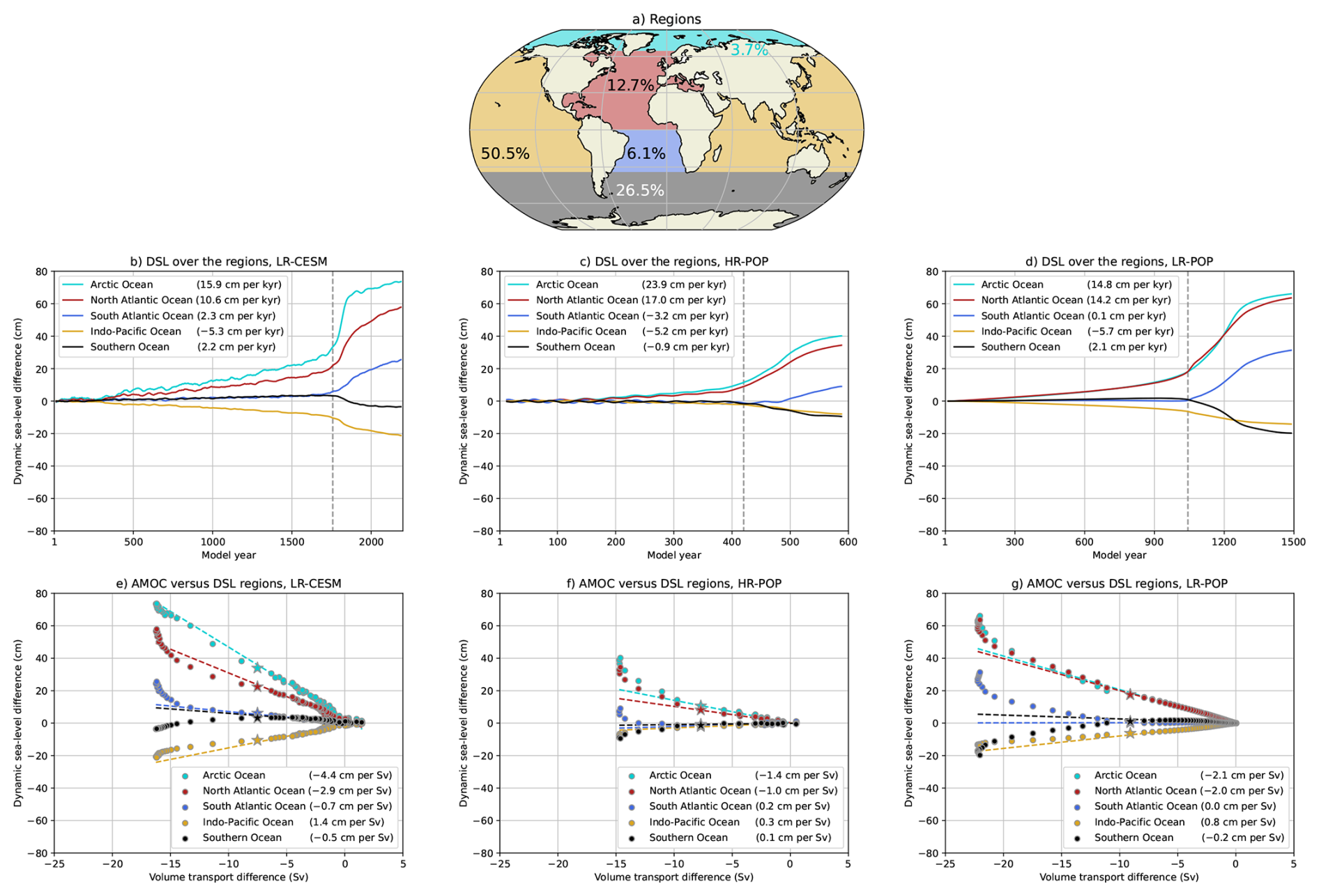
Figure 2 (a) Definition of the five different regions. The percentages indicate the fraction of the total ocean surface, the remaining 0.5 % is attributed to (semi-)enclosed seas and lakes. (b–d) Spatially-averaged DSL over five different regions for the LR-CESM, HR-POP and LR-POP. The DSL time series are displayed as their differences to the first 50 years and are then smoothed through a 25-year running mean to reduce the variability. The vertical gray line marks the onset of the AMOC collapse. The DSL trends are determined from model year 1 up to the AMOC tipping event and given in the legend (ν). (e–g) Relation between AMOC strength and DSL by region for the LR-CESM, HR-POP and LR-POP. The AMOC strength and DSL by region are displayed as their differences to the first 50 years and are shown for 25-year windows, the star marker indicates the window of the onset of the AMOC collapse. A linear fit is determined through these 25-year windows, starting from the first window up to the window with the star marker, and are given in the legend (ϕ).

DSL_i changes are fairly linear up to the AMOC tipping event in the three simulations and, as the timing of the AMOC tipping event differs among the simulations, we determine DSL_i trends for comparison. These trends are indicated here as ${\mathit{\nu }}_i=\frac{\partial {\mathrm{DSL}}_i}{\partial t}$ (or similarly ${\mathit{\nu }}_i=\frac{\partial {\mathrm{DSL}}_i}{\partial F_H}$), where only the part of DSL_i time series prior to the AMOC tipping event is considered (dashed lines in Fig. 2b, c, d). The magnitudes of ν_i, expressed in units of cm per kyr (1 cm kyr⁻¹ = 0.01 mm yr⁻¹), are displayed in the legend of Fig. 2b, c, d. For reference, the spatial DSL differences between the last 50 model years and first 50 model years are shown in Fig. A1a, b, c, which were already presented in van Westen et al. (2024b) and van Westen et al. (2025a).

The Arctic Ocean and North Atlantic Ocean regions have the largest ν in all simulations. For the latter region, the hosing is directly applied over the latitude bands between 20 to 50° N and increases DSLs through freshening. The background circulation (overturning, gyres and eddies) then carries the imposed freshwater flux forcing into the Arctic Ocean (van Westen et al., 2024b; Vanderborght et al., 2025). As the globally-averaged DSL is zero, the increasing DSLs over the North Atlantic Ocean and Arctic Ocean are compensated over the remaining ocean regions. The largest DSL drop is found over the Indo-Pacific Ocean region and is remarkably consistent ($\mathit{\nu }\approx -\mathrm{5.5}$ cm kyr⁻¹) among the simulations. This consistent DSL drop is attributed to the negative freshwater flux forcing to conserve ocean salinity. The magnitude of ν over the two remaining regions (South Atlantic Ocean and Southern Ocean) is relatively small with different ν signs. For example for DSL over the South Atlantic region, the DSL is increasing (LR-CESM), decreasing (HR-POP) or remains near zero (LR-POP). These intermodel differences in ν are attributed to ocean dynamics, as the applied hosing is identical across the simulations.

The largest DSL changes occur during the AMOC collapse, with a pronounced DSL rise over the North Atlantic Ocean and Arctic Ocean. Both regions exhibit large-scale upper-ocean freshening as a consequence of the salt-advection feedback that destabilises the AMOC, as well as cooling due to reduced meridional heat transport by the weakened AMOC (van Westen et al., 2024b; Vanderborght et al., 2025). Freshening decreases ocean density, whereas cooling increases it, however, the freshening dominates when expressed in terms of ocean buoyancy (van Westen et al., 2025d). As a result, upper-ocean densities decrease in these two regions and leading to DSL rise. The collapsing AMOC strongly modifies the meridional freshwater and heat transports over these regions, explaining why their DSL time series closely follow the AMOC strength (compare Figs. 2b, c, d with Fig. 1a).

This DSL-AMOC relation is quantified as: ${\mathit{\varphi }}_i=\frac{\partial {\mathrm{DSL}}_i}{\partial \mathrm{AMOC}}$ (Fig. 2e, f, g). Similar as before, the quantity ϕ_i is determined up to the AMOC tipping event, and the relation is extrapolated to cover the whole range of AMOC strength variations. When the extrapolated ϕ_i reasonably agrees with the modelled AMOC and DSL_i changes, it implies that the DSL_i is strongly related to the AMOC strength through the salt-advection feedback. This is indeed the case for the North Atlantic Ocean and Arctic Ocean for the LR-CESM and LR-POP (Table A1), which is also reflected in their relatively large $\left|\mathit{\varphi }\right|$ values (compared to the remaining three regions). The latter is also the case for the HR-POP, but the AMOC and DSL_i changes match less well with the extrapolated ϕ_i (Table A1). Note that near the end of the simulations, DSL_i still changes while the AMOC has equilibrated (i.e., ΔDSL_i≠0 and ΔAMOC≈0), which is related to F_H variations. Although the HR-POP has the lowest $\left|\mathit{\varphi }\right|$ for the North Atlantic Ocean and Arctic Ocean (compared to the LR-CESM and LR-POP), it has the largest ν for the North Atlantic Ocean (17 cm kyr⁻¹) an Arctic Ocean (23.9 cm kyr⁻¹) and is related to the most sensitive AMOC (i.e., $\frac{\partial \mathrm{AMOC}}{\partial t}$) prior to its collapse. As was argued above, some regions (e.g., Indo-Pacific Ocean) may show an apparent DSL-AMOC relation and is likely explained by balancing effects (−F_H and/or globally-averaged DSL of zero).

The results in Fig. 2 demonstrate that an AMOC collapse influences DSLs. To further quantify these DSL responses under a collapsing AMOC, we determine the linear DSL trends over three 101-year windows: before, during and after the AMOC collapse (Fig. 3). The window length is motivated by the AMOC collapse timescale in the LR-CESM and the fact that hosing effects on DSL are expected to be relatively small over this timescale (ΔF_H=0.03 Sv), which we will make more explicit in Sect. 3.2. Relatively large DSL trends are found over the North Atlantic Ocean and Arctic Ocean during the AMOC collapse (middle row in Fig. 3), with maximum DSL trends reaching +6 mm yr⁻¹. There are also relatively large DSL trends over the Gulf Stream (extension) region which are connected to changes in the Gulf Stream path (van Westen et al., 2025a). In contrast, there are hardly any DSL trends before and after the AMOC collapse (upper and lower rows in Fig. 3, respectively), indicating an acceleration in the DSL rise over the Atlantic sector during the AMOC collapse. The only exception is the HR-POP, which shows DSL trends over the last 101 model years (Fig. 3h) as the AMOC is still adjusting over this period; DSL trends become smaller towards the end of the simulation (Fig. 2c).

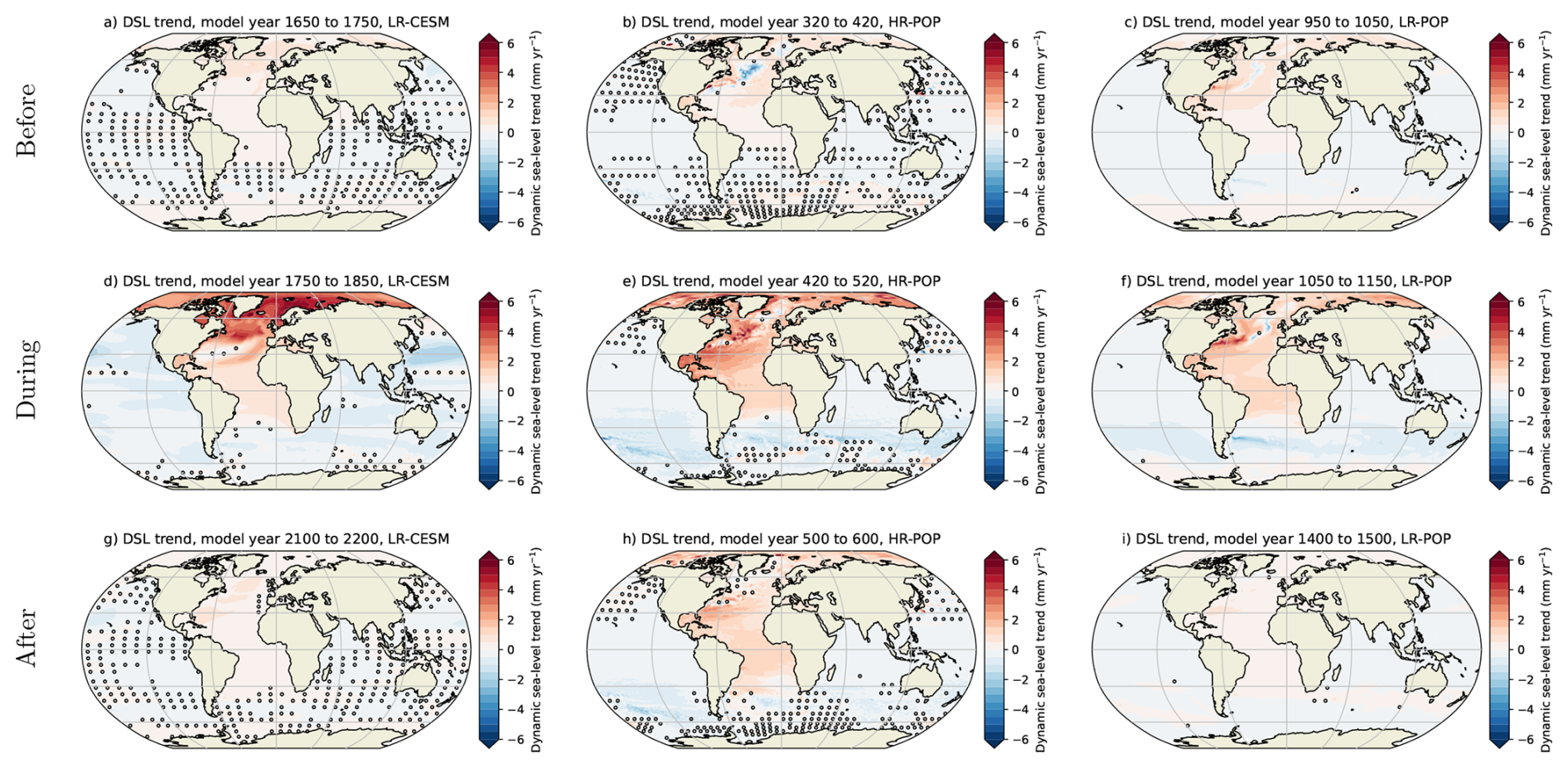
Figure 3 DSL trends over varying 101-year windows for the LR-CESM (left), HR-POP (center) and LR-POP (right), where markers indicate non-significant (p≥0.05) DSL trends. The 101-year windows are (upper row): before the AMOC collapse, (middle row): during the AMOC collapse, and (lower row): after the AMOC collapse (end of simulation).

The collapsing AMOC causes DSL changes along coastal zones in the North Atlantic basin. To quantify these coastal DSL changes, we consider two densely-populated coastal zones in the western part and eastern part of the North Atlantic Ocean. First, the eastern North American coastline starting from Florida and moving northward (Fig. 4a, b, c), where DSL trends during the AMOC collapse and DSL differences (between last and first 50 model years) are shown. DSL is increasing along the North American coastline during the AMOC collapse in all simulations, with DSL trends varying between +1 to +4 mm yr⁻¹. DSLs increase between the last and first 50 model years, but their latitudinal responses greatly vary among the simulations (i.e., compare blue curves in Fig. 4a, b, c) and are attributed to the following contributions. One of the dominant contributions comes from AMOC strength variations, as larger AMOC decline induces more DSL rise over the North Atlantic Ocean (Fig. 2e, f, g). DSL differences increase further north in the LR-CESM and the opposite is true for the LR-POP (and HR-POP), which suggests that climate feedbacks (e.g., changing wind circulation under AMOC strength variations (Mimi and Liu, 2024)) are a relevant contributor. Horizontal ocean resolution also plays a role in modulating DSL responses, illustrated by fairly constant DSL trends with latitude in HR-POP, whereas there are latitudinal variations in the LR-POP (and LR-CESM). Local DSLs are influenced by the Florida Current through geostrophic balance (Levermann et al., 2005) and to realistically resolve this current and its responses, a high-resolution (≤0.1°) ocean component is required (Small et al., 2014). Another important and non-negligible contribution comes from the imposed freshwater flux forcing, which will be addressed in Sect. 3.2 for the LR-CESM.

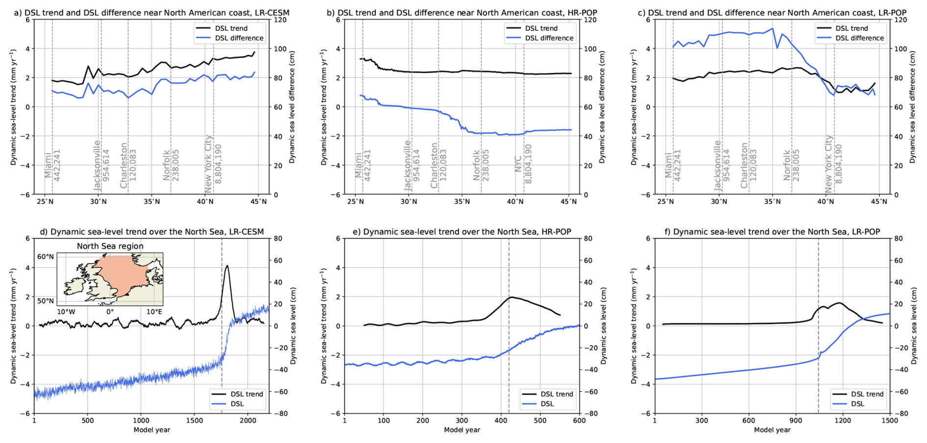
Figure 4 (a–c) DSL changes along the eastern North American coastline (i.e., ocean grid cells closest to the coast) for the LR-CESM, HR-POP and LR-POP, displaying DSL trends during the AMOC collapse (black curve, left vertical axis) and DSL differences between the last and first 50 model years (blue curve, right vertical axis). The 101-year windows for the DSL trends are model years 1750–1850 (LR-CESM), 420–520 (HR-POP), and 1050–1150 (LR-POP), the spatial patterns were shown in Fig. 3d, e, f. Five different coastal cities are indicated with their resident population (based on the 2020 Census). (d–f) The spatially-averaged DSL trend (black curve, left vertical axis) and DSL (blue curve, right vertical axis) over the North Sea for the LR-CESM, HR-POP and LR-POP, the outlined region in panel (d) indicates the North Sea. The DSL trends are determined over 101-year sliding windows. The dashed gray line indicates the onset of the AMOC collapse.

Second, we examine the spatially-averaged DSL changes over the North Sea region (see inset in Fig. 4d), which is located in the eastern part of the North Atlantic Ocean. This semi-enclosed basin is a relatively shallow sea, with an average depth of about 100 m, and its northern boundary and southwestern boundary are connected to the North Atlantic Ocean. Sea-level variations are caused by local and remote drivers here (Dangendorf et al., 2014; Hermans et al., 2020). In the LR-CESM and LR-POP, the North Sea region is represented by only 170 grid points (≈50 km horizontal resolution), whereas the HR-POP includes significantly more grid points, totalling to 9784 grid points (≈7.5 km horizontal resolution). The surface of the North Sea region receives the compensating (i.e., negative) freshwater flux forcing, but DSL does rise in all the simulations (blue curves in Fig. 4d, e, f) as the Atlantic Ocean circulation transports the imposed freshwater anomalies (between 20 to 50° N) into the North Sea region. There is a substantial acceleration in DSL rise during the AMOC collapse (black curves in Fig. 4d, e, f), with DSL trends reaching +4.15 mm yr⁻¹ in the LR-CESM, demonstrating that the DSL over the North Sea is strongly influenced by the AMOC.

In summary, this section presented DSL changes under a collapsing AMOC in the LR-CESM, HR-POP and LR-POP. DSLs over the North Atlantic Ocean and Arctic Ocean are influenced most under an AMOC collapse. Note that the DSL changes between the start and end of the simulations have a (substantial) hosing contribution, which will now be discussed in the section below.

3.2 The hosing-corrected dynamic sea level responses

The slowly-increasing freshwater flux forcing triggers the AMOC tipping event and a weaker AMOC causes DSL redistribution (Sect. 3.1). One unintended effect of the hosing is that it induces DSL changes through density variations. To isolate the “pure” AMOC collapse effects to DSL changes, we analyse the accompanying backward quasi-equilibrium LR-CESM simulation (Fig. 5a); this backward simulation was not performed for the HR-POP and LR-POP (see Methods). When lowering the freshwater flux forcing, the AMOC starts to recover from model year 4090 (F_H=0.093 Sv) and onwards, resulting in a multi-stable AMOC regime between F_H=0.093 Sv to F_H=0.527 Sv. DSL trends during the AMOC recovery (model year 4090 to 4190, Fig. A2) are opposite to the ones during the AMOC collapse, the AMOC recovery results are not further discussed here. To remove the hosing contribution to DSL, one needs to subtract the different oceanic states (i.e., “AMOC off” minus “AMOC on”) for the same F_H in the multi-stable AMOC regime.

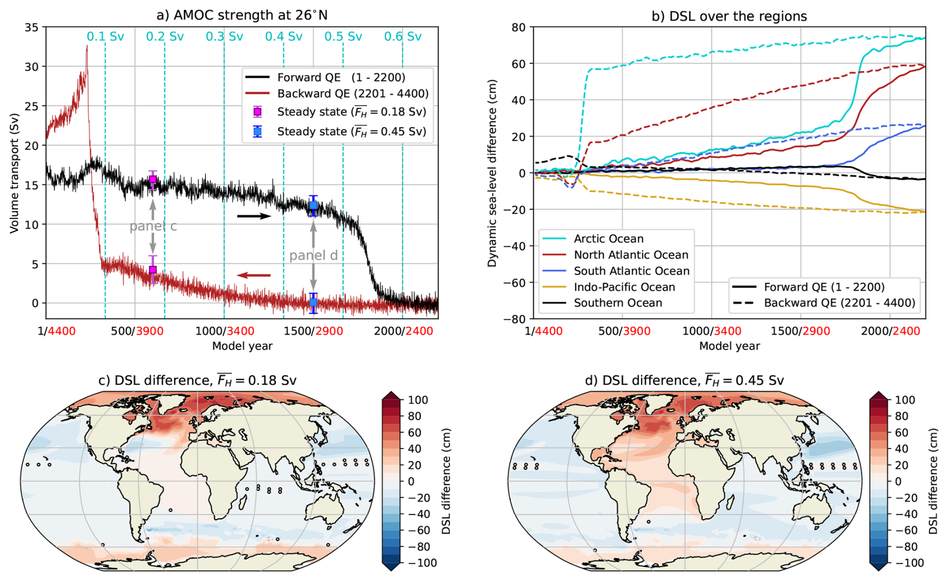
Figure 5 (a) The AMOC strength at 1000 m and 26° N for the forward (black curve) and backward (red curve) quasi-equilibrium LR-CESM. Markers indicate the statistical equilibria (i.e., steady states) for $\stackrel{\mathrm{‾}}{F_H}=\mathrm{0.18}$ Sv and $\stackrel{\mathrm{‾}}{F_H}=\mathrm{0.45}$ Sv, including error bars for their minimum and maximum values. (b) Spatially-averaged DSL differences (compared to the first 50 model years) over the five different regions (cf. Fig. 2a), where solid (dashed) curves indicates the forward (backward) quasi-equilibrium LR-CESM. The time series are smoothed through a 25-year running mean to reduce the variability. (c, d) DSL differences between the statistical equilibria for $\stackrel{\mathrm{‾}}{F_H}=\mathrm{0.18}$ Sv and $\stackrel{\mathrm{‾}}{F_H}=\mathrm{0.45}$ Sv, displayed as the “AMOC off” state minus the “AMOC on” state. The markers indicate non-significant (p≥0.05) DSL differences.

The spatially-averaged DSL over the five regions in the full QE LR-CESM are presented in Fig. 5b, which also display hysteresis behaviour. We first consider the North Atlantic Ocean region, the region that receives the hosing between 20 to 50° N. As was argued in Sect. 3.1, ocean dynamics under the AMOC collapse induce DSL rise over the North Atlantic Ocean. In the backward QE simulation, the AMOC strength remains 0 Sv between model year 2200 to 3200 ($\mathrm{\Delta }{F}_H=-\mathrm{0.3}$ Sv, Fig. 5a) and we therefore assume that the contribution of ocean dynamics on DSL remains constant over this period. Hence, the North Atlantic DSL decline of 19.3 cm is attributed to decreasing F_H over this period (dashed red curve in Fig. 5b), resulting in a DSL sensitivity of 64 cm per Sv hosing. The total hosing contribution to North Atlantic DSL then yields 42 cm (ΔF_H=0.66 Sv) and accounts for 70 % of the 60 cm of North Atlantic DSL rise by model year 2200 (at F_H=0.66 Sv). The remaining 20 cm is attributed to different AMOC regimes, which roughly corresponds to the North Atlantic DSL differences for the same F_H in the multi-stable AMOC regime (compare the red solid and dashed curves in Fig. 5b). Conversely, the hosing contribution to North Atlantic DSL during the AMOC collapse (ΔF_H=0.03 Sv, Figs. 2b and 3d) is quite small (1.9 cm), confirming our earlier assumption that DSL changes during the AMOC collapse are primarily caused internal ocean dynamics. The magnitudes of DSL sensitivity under hosing for the remaining regions are lower than the North Atlantic Ocean (Table A2), demonstrating that the North Atlantic Ocean is most sensitive under varying F_H, which is expected as the hosing is directly applied over this region.

The spatial DSL patterns between “AMOC off” minus “AMOC on” are presented in Fig. 5c and d for $\stackrel{\mathrm{‾}}{F_H}=\mathrm{0.18}$ Sv and $\stackrel{\mathrm{‾}}{F_H}=\mathrm{0.45}$ Sv, respectively. These DSL changes are corrected for the hosing contribution and their overall patterns and amplitudes are quite similar between $\stackrel{\mathrm{‾}}{F_H}=\mathrm{0.18}$ Sv and $\stackrel{\mathrm{‾}}{F_H}=\mathrm{0.45}$ Sv, with Table A2 displaying the hosing-corrected DSL differences per region. There are, however, some notable differences over the North Atlantic subtropical gyre, which show declining DSLs for $\stackrel{\mathrm{‾}}{F_H}=\mathrm{0.18}$ Sv and increasing DSLs for $\stackrel{\mathrm{‾}}{F_H}=\mathrm{0.45}$ Sv. These differences are likely not related to AMOC strength variations, as $\stackrel{\mathrm{‾}}{F_H}=\mathrm{0.18}$ Sv and $\stackrel{\mathrm{‾}}{F_H}=\mathrm{0.45}$ Sv have comparable AMOC strength differences (“AMOC on” minus “AMOC off”) of 11.5 and 12.3 Sv, respectively (Figure 5a). DSL differences over the North Atlantic subtropical gyre can be explained by the sea surface salinity changes there; sea surface temperature responses are quite similar (Fig. A3). Sea surface salinities over the subtropical gyre are increasing (i.e., lower DSLs) between “AMOC off” and “AMOC on” for $\stackrel{\mathrm{‾}}{F_H}=\mathrm{0.18}$ Sv, while decreasing (i.e., higher DSLs) for $\stackrel{\mathrm{‾}}{F_H}=\mathrm{0.45}$ Sv. There is also salinity accumulation over the subtropical gyre at subsurface depths (250–500 m) for lower values of F_H and collapsed AMOC state (van Westen and Dijkstra, 2023). The different North Atlantic salinity responses between $\stackrel{\mathrm{‾}}{F_H}=\mathrm{0.18}$ Sv and $\stackrel{\mathrm{‾}}{F_H}=\mathrm{0.45}$ Sv can be linked to the overturning circulation in the “AMOC off” state. There is a weak and shallow (<1000 m) overturning cell from 34° S to 40° N for the $\stackrel{\mathrm{‾}}{F_H}=\mathrm{0.18}$ Sv case (van Westen and Dijkstra, 2023), which transports salinity anomalies northward and causes salinity accumulation over the North Atlantic subtropical gyre (Fig. A3c). On the other hand, there is no overturning cell for the $\stackrel{\mathrm{‾}}{F_H}=\mathrm{0.45}$ Sv case (van Westen and Dijkstra, 2023) and freshwater anomalies spread over the entire Atlantic Ocean surface (Fig. A3d). DSL, sea surface temperature and sea surface salinity are comparable north of 40° N (Figs. 5c, d and A3), as the residual overturning cell in the “AMOC off” regime vanishes north of 40° N (van Westen and Dijkstra, 2023). Depending on the residual overturning circulation in the “AMOC off” regime, one can expect (substantially) different Atlantic DSL responses between 34° S to 40° N.

DSL changes along the North American coastline are also influenced under the residual overturning circulation in the “AMOC off” regime, with smaller DSL rise (up to 40° N) in the $\stackrel{\mathrm{‾}}{F_H}=\mathrm{0.18}$ Sv case compared to the $\stackrel{\mathrm{‾}}{F_H}=\mathrm{0.45}$ Sv case (Fig. 6a, b). For the North Sea region, which is located north of 40° N, DSL increases by about 50 cm for both $\stackrel{\mathrm{‾}}{F_H}=\mathrm{0.18}$ Sv and $\stackrel{\mathrm{‾}}{F_H}=\mathrm{0.45}$ Sv (Fig. 6c, d). When comparing DSL changes in the forward QE LR-CESM (between the last and first 50 model years, Fig. 4) with those of the hosing-corrected DSL changes (Fig. 6), local DSL changes can be overestimated by 60 cm in the QE LR-CESM. Consequently, interpreting DSL changes demands careful attention to hosing conditions and state-dependent responses.

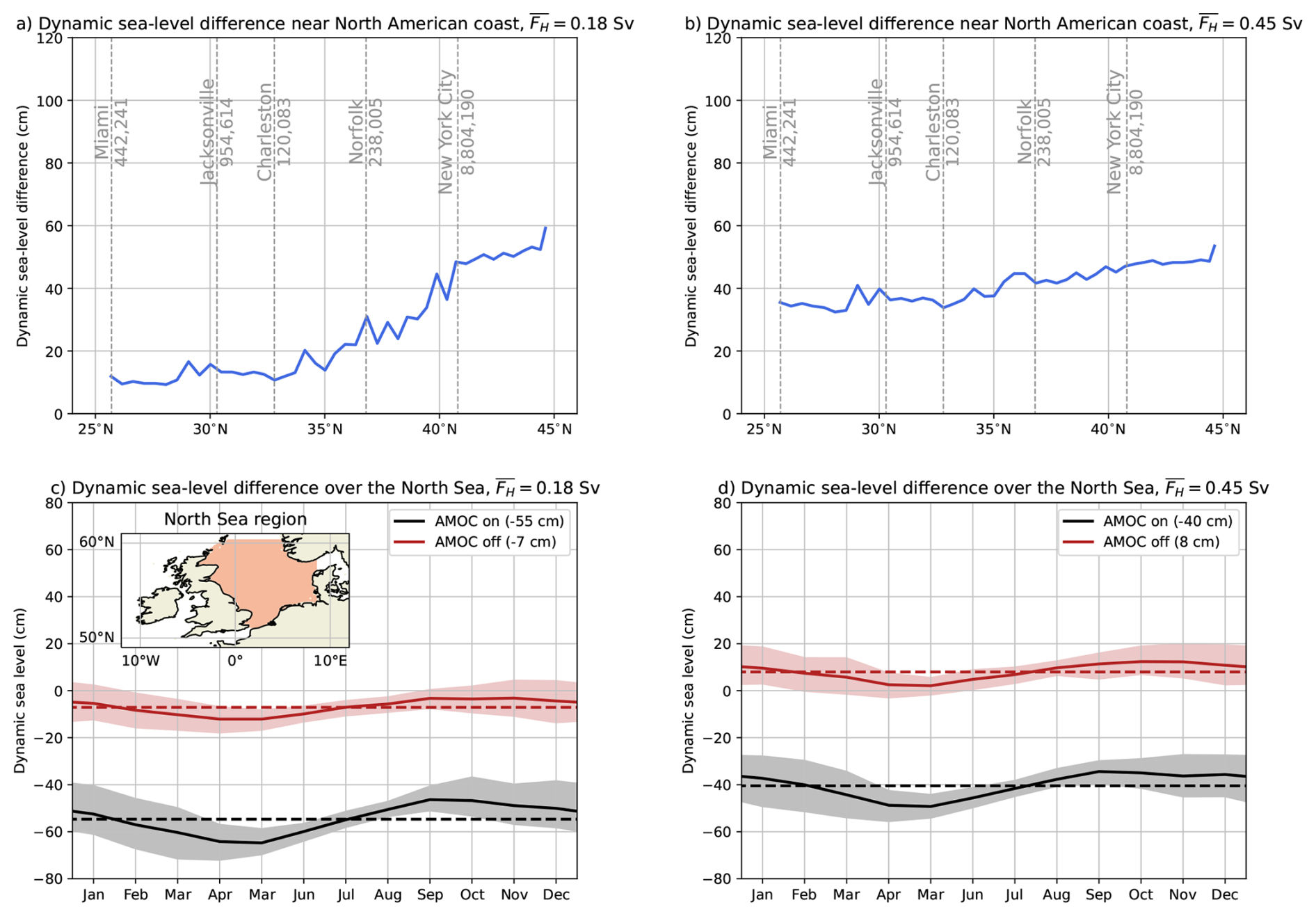
Figure 6 (a, b) DSL differences along the North American coastline (i.e., ocean grid cells closest to the coast) for the statistical equilibria of $\stackrel{\mathrm{‾}}{F_H}=\mathrm{0.18}$ Sv and $\stackrel{\mathrm{‾}}{F_H}=\mathrm{0.45}$ Sv for the LR-CESM, displayed as “AMOC off” minus “AMOC on”. Five different coastal cities are indicated with their resident population (based on the 2020 Census). (c, d) Spatially-averaged DSL climatology over the North Sea (see inset panel (c)) for the statistical equilibria of $\stackrel{\mathrm{‾}}{F_H}=\mathrm{0.18}$ Sv and $\stackrel{\mathrm{‾}}{F_H}=\mathrm{0.45}$ Sv for the LR-CESM. The shading indicates the 5 % and 95 % percentiles, the dashed lines are time-mean DSLs and are indicated in the legend.

Finally, we determine the hosing-corrected DSL trends during the AMOC collapse using the backward QE simulation. The AMOC collapses between model years 1750 and 1850 (ΔF_H=0.03 Sv), with the corresponding period occurring between model years 2550 and 2650 ($\mathrm{\Delta }{F}_H=-\mathrm{0.03}$ Sv) in the backward QE simulation. These DSL trends in the backward QE mainly represent the varying F_H contribution to DSL, as the AMOC strength remains at 0 Sv and, for convenience, we reverse the sign of the DSL trends to mimic increasing F_H values (Fig. 7a). The largest hosing-induced DSL trends are found over the subtropical gyre, with magnitudes of +0.4 mm yr⁻¹, which can locally be larger than the uncorrected DSL trends (see Fig. 3d). North of the subtropical gyre, the hosing-induced DSL trends are typically +0.2 mm yr⁻¹ and are substantially smaller than the uncorrected DSL trends. For example over the North Sea, the maximum DSL trend is +4.15 mm yr⁻¹ (uncorrected) and reduces to +3.97 mm yr⁻¹ (hosing-corrected), a reduction of about 4 %. This is also reflected in comparable patterns and amplitudes between the uncorrected (Fig. 3d) and hosing-corrected (Fig. 7b) DSL trends.

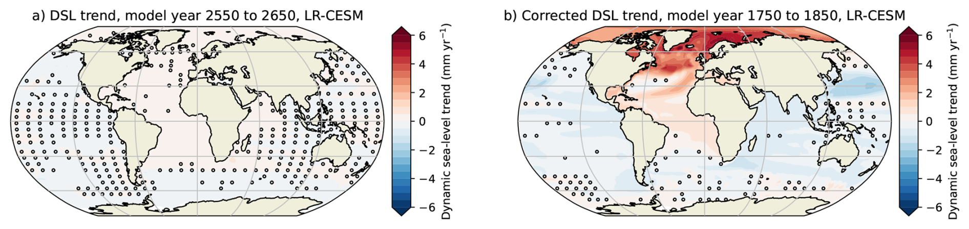
Figure 7 (a) DSL trends over model years 2550–2650 for the LR-CESM. Note that the sign of the DSL trends is reversed. (b) The hosing-corrected DSL trends for model years 1750–1850 for the LR-CESM. Markers indicate non-significant (p≥0.05) DSL trends.

4 Results – Steric sea-level responses

In this second result section, we explore steric sea-level changes under a collapsing AMOC. In Sect. 4.1, the globally-averaged steric sea-level changes are analysed, which are primarily caused by oceanic temperature changes (i.e., thermosteric sea-level rise, ${\mathit{\eta }}_{\mathrm{s}}^{\mathrm{g}}$) as salinity is conserved under the varying freshwater flux forcing. In Sect. 4.2, the sterodynamic sea-level responses (SDSL = DSL + ${\mathit{\eta }}_{\mathrm{s}}^{\mathrm{g}}$) are presented, where we will focus on the hysteresis simulation with the LR-CESM.

4.1 Thermosteric sea-level responses under a collapsing AMOC

The thermosteric sea-level changes for the three forward QE hosing simulations are displayed in Fig. 8a. Both the LR-CESM and HR-POP display qualitatively similar ${\mathit{\eta }}_{\mathrm{s}}^{\mathrm{g}}$ trajectories: prior to the AMOC tipping event ${\mathit{\eta }}_{\mathrm{s}}^{\mathrm{g}}$ decreases and is followed by a strong increase. For the LR-POP, on the other hand, ${\mathit{\eta }}_{\mathrm{s}}^{\mathrm{g}}$ first rises and, once the AMOC starts to collapse, it strongly decreases.

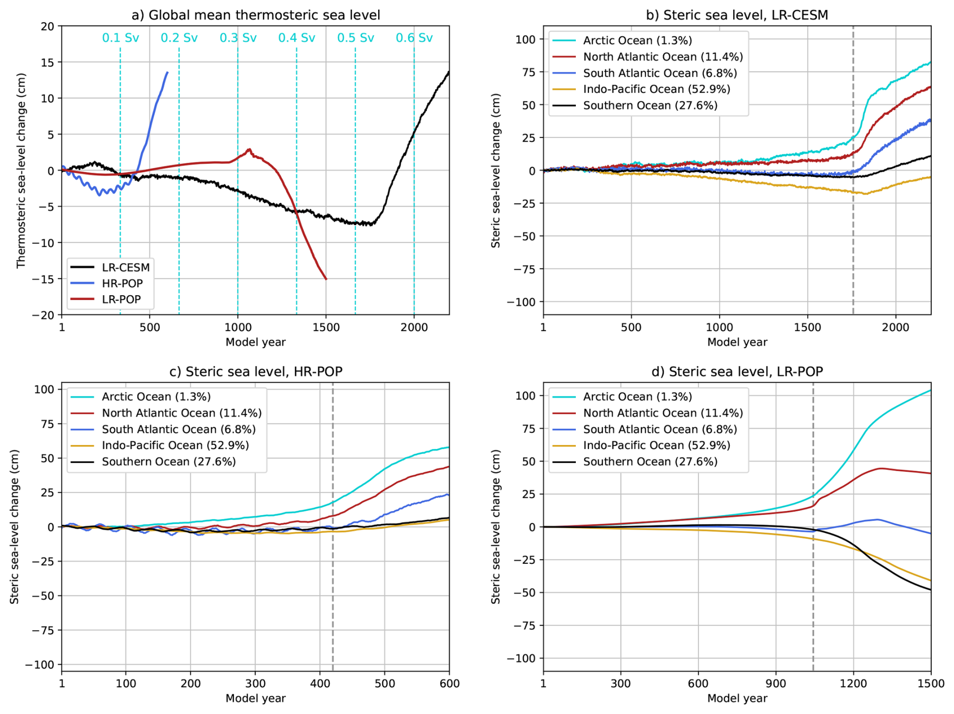
Figure 8 (a) The globally-averaged thermosteric sea-level change (${\mathit{\eta }}_{\mathrm{s}}^{\mathrm{g}}$, compared to first 50 model years) for the LR-CESM, HR-POP and LR-POP. (b–d) The steric sea-level changes (compared to first 50 model years) over the five different regions for the (b) LR-CESM, (c) HR-POP, and (d) LR-POP. The dashed gray line indicates the onset of the AMOC collapse. The percentages in the legend indicate the fraction of the total ocean volume (with (semi-)enclosed seas and lakes only accounting for 0.06 %).

It is interesting to understand these ${\mathit{\eta }}_{\mathrm{s}}^{\mathrm{g}}$ trajectories and the role of the collapsing AMOC in the LR-CESM, HR-POP and LR-POP. For example, the AMOC downwells heat (and salt) into the deep ocean, and an AMOC collapse could alter oceanic heat uptake and storage, where the latter then induces thermosteric sea-level changes. However, oceanic heat uptake is strongly controlled by the stratification over the North Atlantic Ocean and Southern Ocean, and not so much by the AMOC (Gregory et al., 2024; Vogt et al., 2025). As the stratification over the North Atlantic Ocean and Southern Ocean sets the AMOC strength (assuming thermal wind balance and adiabatic limit) through their shared interior isopycnals (Nikurashin and Vallis, 2012; Wolfe and Cessi, 2014), an apparent relation between AMOC strength and oceanic heat uptake emerges. Nevertheless, an AMOC collapse (in)directly influences the stratification over the North Atlantic Ocean and Southern Ocean, as there are no shared isopcynals between the regions (van Westen et al., 2025d), and is also reflected in deeper mixed layer depths over the Southern Ocean (van Westen et al., 2024b). These oceanic responses could then influence oceanic heat uptake and storage (upper row in Fig. A4) and, from this, thermosteric sea-level changes.

The ${\mathit{\eta }}_{\mathrm{s}}^{\mathrm{g}}$ is decomposed into steric sea-level contributions for the five different regions and for the LR-CESM, HR-POP, and LR-POP (Fig. 8b, c, d). Do note that both temperature (Fig. A4) and salinity (Fig. A5) change influence the steric sea-level responses. After the onset of the AMOC collapse, steric sea levels are increasing over all five regions for both the LR-CESM (Fig. 8b) and HR-POP (Fig. 8c). However for the LR-POP (Fig. 8d), only the South Atlantic Ocean, North Atlantic Ocean, and Arctic Ocean are rising after the onset of the AMOC collapse. Steric sea-levels for the South Atlantic Ocean and North Atlantic Ocean slightly drop after model year 1300, which appear to be related to the development of a reversed AMOC (red curve in Fig. 1a). Steric sea levels over the Indo-Pacific Ocean and Southern Ocean drop after the AMOC collapse in LR-POP, which explain the different ${\mathit{\eta }}_{\mathrm{s}}^{\mathrm{g}}$ trajectory between the LR-POP with that of the LR-CESM and HR-POP (Fig. 8a).

Changes in ${\mathit{\eta }}_{\mathrm{s}}^{\mathrm{g}}$ are related to net heat exchange with the atmosphere. The globally-averaged surface heat flux is shown in Fig. 9a, b, c (purple curves) for the LR-CESM, HR-POP and LR-POP, which is initially close to zero meaning that the ocean is in near equilibrium. The surface heat fluxes over the five regions are also displayed in Fig. 9a, b, c. Do note that horizontal heat exchange between the regions also influences oceanic temperatures. For example for the LR-CESM, the surface heat flux over the Indo-Pacific Ocean remains fairly constant (yellow curve in Fig. 9a) while its volume-averaged temperature is increasing (yellow curve in Fig. A4a), meaning that there is net horizontal convergence of heat into the Indo-Pacific Ocean. The most striking difference is found for the North Atlantic Ocean (red curves in Fig. 9a, b, c), which initially loses heat and, after the AMOC collapse, gains heat from the atmosphere. The intermodel surface heat flux changes are also comparable for the South Atlantic Ocean (blue curves, less heat uptake), Arctic Ocean (cyan curves, less heat loss), and Indo-Pacific Ocean (yellow curves, remains fairly constant). The Southern Ocean (black curve) loses more heat after the AMOC collapse in all simulations, with the LR-POP displaying much larger responses (≈ factor of 5) compared to the LR-CESM and HR-POP. The spatial patterns in surface heat flux differences are indeed quite similar (Fig. 9d, e, f), with the exception of the Southern Ocean in the LR-POP. These Southern Ocean surface heat flux responses in LR-POP highlight again differences with the LR-CESM and HR-POP, which do contribute to intermodel ${\mathit{\eta }}_{\mathrm{s}}^{\mathrm{g}}$ differences (Fig. 8a).

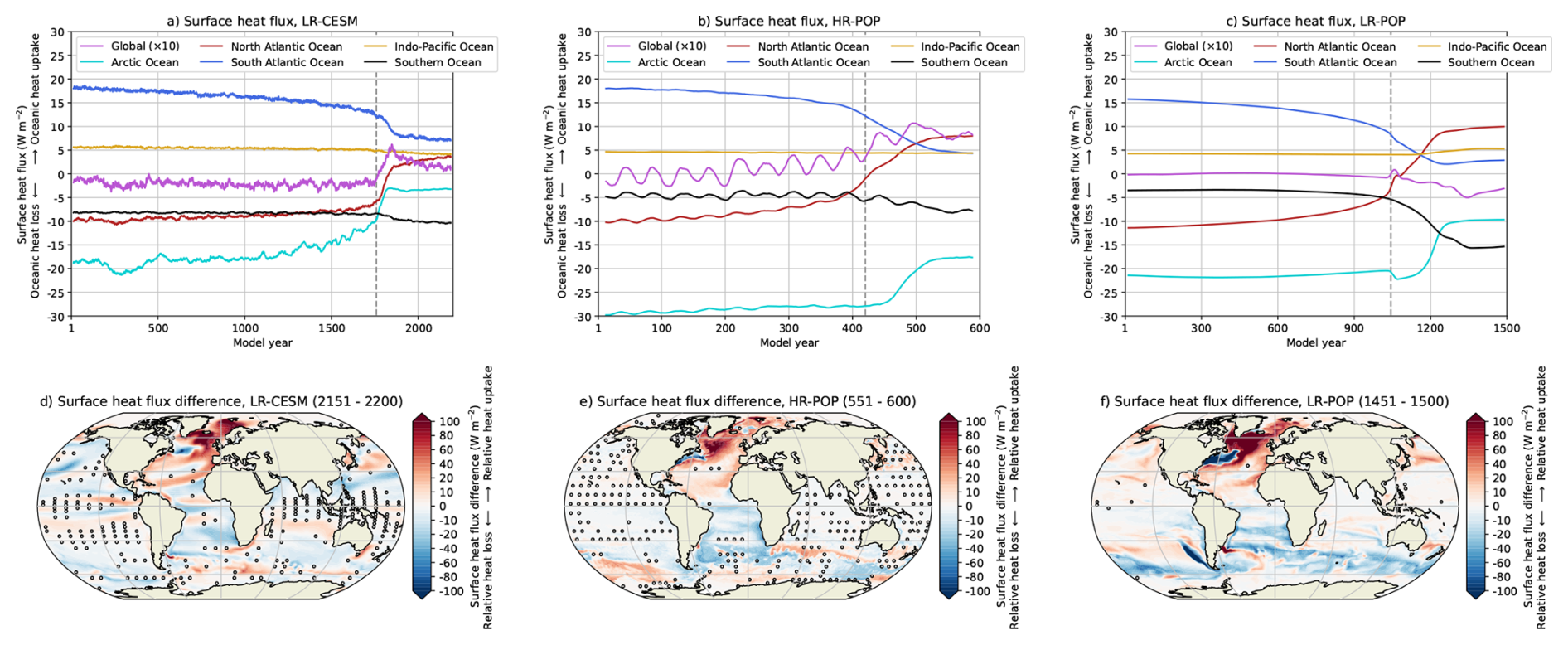
Figure 9 (a–c) The surface heat flux over the different regions and the global average (multiplied by factor 10) for the LR-CESM, HR-POP and LR-POP. The time series are smoothed through a 25-year running mean to reduce the variability. The dashed gray line in all the panels indicates the onset of the AMOC collapse. (d–f) The surface heat flux difference (last 50 minus first 50 model years) for the LR-CESM, HR-POP and LR-POP. The markers indicate non-significant (p≥0.05) surface heat flux differences.

The surface heat flux responses over the Southern Ocean are quite different when comparing the HR-POP (Fig. 9e) and LR-POP (Fig. 9f), while both simulations have the same prescribed atmosphere. This difference is attributed to ocean eddies, which are crucial for the Southern Ocean momentum balance and oceanic responses (Stewart and Hogg, 2017; van Westen and Dijkstra, 2021). Following the AMOC collapse, the Southern Ocean isopycnal slopes adjust and influence the Southern Ocean eddy field (Smolders et al., 2026). Wind are prescribed and hence do not contribute to any ocean eddy field changes. The HR-POP shows both positive and negative anomalies in sea surface temperature and mixed layer depth over the Southern Ocean (see Fig. 4 in van Westen et al., 2025a), while the LR-POP only shows increasing sea surface temperatures and mixed layer depths (see Fig. S6 in van Westen et al., 2025a). The sea surface temperature responses eventually control the sign of surface heat flux changes, as higher (lower) sea surface temperatures increase (decrease) the temperature difference with the overhead atmosphere and result in greater (smaller) heat loss over the Southern Ocean. The interaction between ocean eddies with the Antarctic Circumpolar Current also induces a mode of Southern Ocean multidecadal variability (40–50 years) that propagates through the global ocean (Le Bars et al., 2016; van Westen and Dijkstra, 2017) and is visible in the HR-POP time series (e.g., Figs. 8a, c and 9b). A limitation of both HR-POP and LR-POP is their prescribed atmosphere, which effectively implies an infinite atmospheric heat capacity (Le Bars et al., 2016). Hence, the LR-CESM needs to be analysed to consider the energy balance of the entire climate system.

The total energy budget of the Earth system can be quantified by analysing the radiative imbalance at the top of atmosphere (TOA, Fig. 10a). The responses at TOA are comparable to the globally-averaged surface heat fluxes (purple curve in Fig. 9a), meaning that AMOC strength variations modulate the surface heat fluxes and this is followed by adjustments in the TOA radiative imbalance. There is a small residual between the surface heat fluxes and TOA radiative imbalance, with the residual being stored/released by the atmosphere. Therefore, we determine both the volume-averaged oceanic temperature and the mass-weighted atmospheric temperature to quantify heat budget changes. Before the AMOC collapse, the TOA imbalance is slightly negative ($\approx -\mathrm{0.1}$ W m⁻²) and this means that the climate system is losing net heat. Both the ocean and atmosphere are losing heat, with a volume-averaged ocean temperature decline of 0.15 °C (Fig. A4a) and a mass-weighted atmospheric temperature decline of 0.06 °C (not shown). The net oceanic cooling results in a thermometric sea-level drop of 7.5 cm prior to the AMOC collapse (Fig. 8a). After the AMOC collapse, the TOA imbalance strongly increases with maximum values of about +0.5 W m⁻² in model year 1850 and then slowly starts to equilibrate to the collapsed AMOC state. This positive energy imbalance is stored in the ocean with a volume-averaged temperature increase of 0.39 °C ($\mathrm{\Delta }{\mathit{\eta }}_{\mathrm{s}}^{\mathrm{g}}=\mathrm{21}$ cm) over the same period, while the mass-weighted atmospheric temperature further drops by 0.19 °C. These results also highlight the dominant role of oceanic heat changes in modulating Earth’s energy balance.

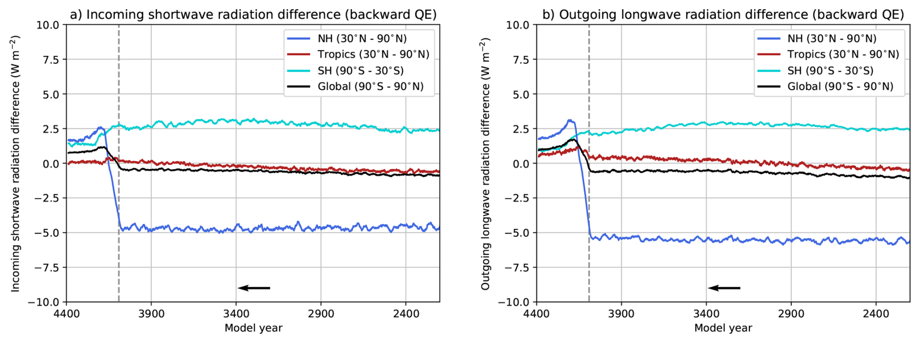
To further understand the abrupt net energy input during the onset of the AMOC collapse, we decompose the TOA radiative imbalance into its incoming shortwave radiation (SWⁱⁿ, Fig. 10b) contribution and outgoing longwave radiation (LW^out, Fig. 10c) contribution. Under an AMOC collapse, both the globally-averaged SWⁱⁿ and LW^out at the TOA decline, although inter-hemispheric differences remain. The SWⁱⁿ decreases over the Northern Hemisphere by the higher surface albedo (primarily due to greater sea-ice cover) and the opposite is true for the Southern Hemisphere, but the Northern Hemispheric albedo response dominates and there is a net increase in the planetary albedo (van Westen et al., 2024b). Consequently, the Northern Hemisphere cools and emits less longwave radiation (i.e., the Planck feedback) and again the opposite is true for the Southern Hemisphere. The globally-averaged response in LW^out is slightly stronger than in SWⁱⁿ, resulting in the positive radiative imbalance at TOA during and after the AMOC collapse. Note that there are also regional climate feedbacks that alter the local radiative imbalance, such as the southward migration of the Intertropical Convergence Zone (ITCZ) that is visible in both SWⁱⁿ and LW^out components (Fig. 10e, f), but not so much in the radiative imbalance (Fig. 10d).

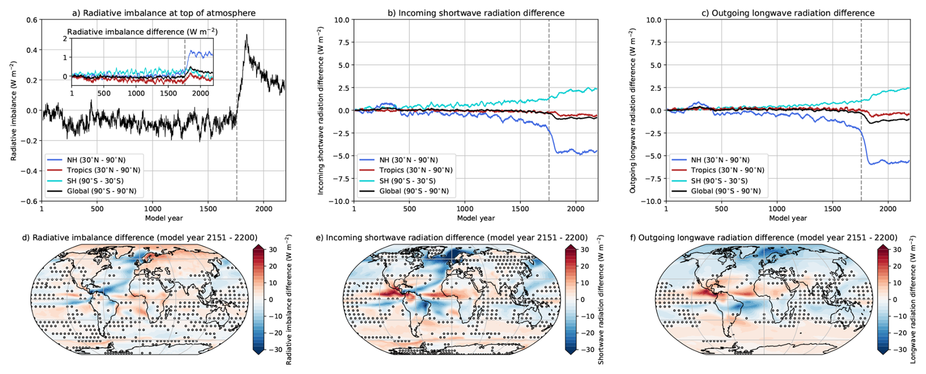
Figure 10 (a–c) The globally-averaged radiative imbalance at the top of atmosphere (a) for the LR-CESM. The inset shows the radiative imbalance difference compared to first 50 model years, which is also split for different latitude bands. The radiative imbalance is decomposed into an incoming shortwave radiation (SWⁱⁿ, panel (b)) contribution and outgoing longwave radiation (LW^out, panel (c)) contribution. The SWⁱⁿ and LW^out time series are displayed as differences (compared to the first 50 model years) and for different latitude bands. All time series are smoothed through a 25-running mean to reduce the variability. The dashed gray line indicates the onset of the AMOC collapse. (d–f) The radiative imbalance at top of atmosphere, SWⁱⁿ and LW^out differences for model years 2151–2200 (compared to first 50 model years). The markers indicate non-significant (p≥0.05) differences.

A collapsing AMOC affects DSLs (Sect. 3), steric sea levels, surface heat fluxes and Earth's energy imbalance. These changes are dependent on horizontal resolution used (strongly eddying versus eddy parametrisation) and configuration used (coupled versus stand-alone ocean). In the coupled simulation (LR-CESM), the findings presented in this section demonstrate that an AMOC collapse leads to a substantial thermosteric sea-level rise (>20 cm), driven by increased oceanic heat uptake. This does not contradict the findings by Gregory et al. (2024) and Vogt et al. (2025), where they argue that the AMOC strength and oceanic heat uptake are not related. Indeed, when the AMOC reduces to zero in the LR-CESM, it effectively halts downwelling of heat in the Atlantic Ocean. Net oceanic heat uptake is ultimately stored in regions outside the Atlantic Ocean (Fig. A4a), underscoring the key role of the AMOC in modulating Earth’s energy balance.

4.2 Sterodynamic sea-level responses

In this last result section, we analyse the resulting SDSL (= ${\mathit{\eta }}_{\mathrm{s}}^{\mathrm{g}}$ + DSL) responses. For the LR-CESM and HR-POP, the increasing ${\mathit{\eta }}_{\mathrm{s}}^{\mathrm{g}}$ contribution during and after the AMOC collapse (Fig. 8a) exacerbates the earlier reported DSL responses over the North Atlantic Ocean and Arctic Ocean. The opposite is true for the LR-POP, which shows declining ${\mathit{\eta }}_{\mathrm{s}}^{\mathrm{g}}$ values during the AMOC collapse. The comparison between DSL and SDSL is shown in Fig. A1 between the end and begin of the forward QE simulations, note that both the DSL and SDSL fields have the unintended hosing effect. It is, however, far more relevant to analyse the full QE hysteresis simulation of the LR-CESM, as Earth’s energy balance can be determined and the climate further equilibrates to its collapsed AMOC state beyond model year 2200. The ${\mathit{\eta }}_{\mathrm{s}}^{\mathrm{g}}$ and TOA radiative imbalance over the full hysteresis simulation are displayed in Fig. 11a, b, respectively.

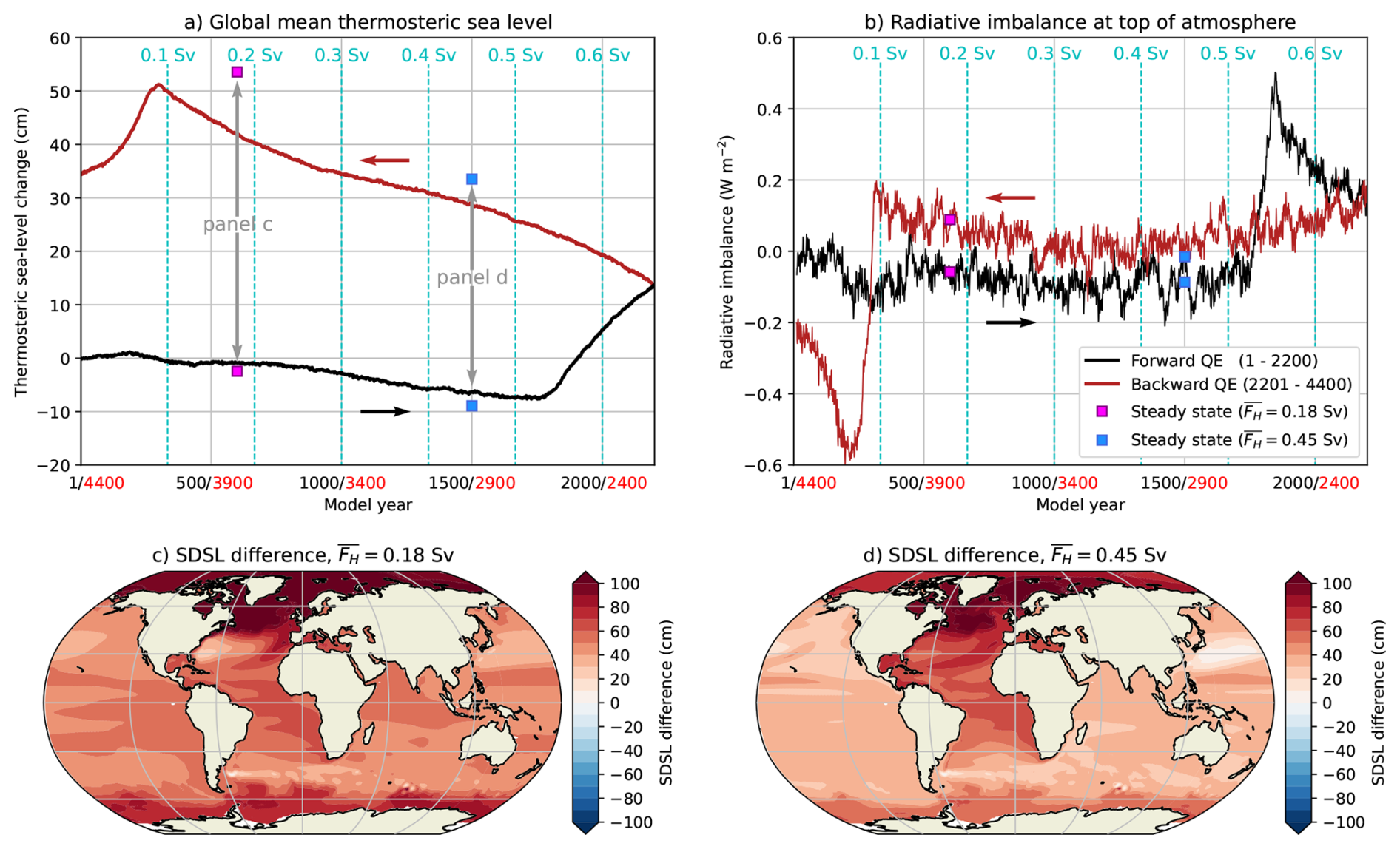
Figure 11 (a) The globally-averaged thermosteric sea-level change (${\mathit{\eta }}_{\mathrm{s}}^{\mathrm{g}}$, compared to first 50 model years) for the forward (black curve) and backward (red curve) quasi-equilibrium LR-CESM. Markers indicate the statistical equilibria (i.e., steady states) for $\stackrel{\mathrm{‾}}{F_H}=\mathrm{0.18}$ Sv and $\stackrel{\mathrm{‾}}{F_H}=\mathrm{0.45}$ Sv (for legend, see panel (b)). (b) Similar to panel (a), but now for the globally-averaged radiative imbalance at the top of atmosphere. The time series is smoothed through a 25-running mean to reduce the variability. (c, d) SDSL differences between the statistical equilibria for $\stackrel{\mathrm{‾}}{F_H}=\mathrm{0.18}$ Sv and $\stackrel{\mathrm{‾}}{F_H}=\mathrm{0.45}$ Sv, displayed as the “AMOC off” state minus the “AMOC on” state. All SDSL differences are significant (p<0.05).

The ${\mathit{\eta }}_{\mathrm{s}}^{\mathrm{g}}$ increases by 14 cm (compared to the first 50 model years) with a remaining TOA imbalance of about +0.15 W m⁻² by model year 2200 (F_H=0.66 Sv). The climate system equilibrates to the “AMOC off” state in the following 1200 years, with the TOA imbalance reaching 0 W m⁻² and ${\mathit{\eta }}_{\mathrm{s}}^{\mathrm{g}}$ rise of 34 cm in model year 3400 (F_H=0.30 Sv). Then, the TOA imbalance slightly increases again up to the AMOC recovery event in model year 4,090 (F_H=0.093 Sv), with a maximum ${\mathit{\eta }}_{\mathrm{s}}^{\mathrm{g}}$ increase of 51 cm. This increase in the TOA imbalance is related to the development of a weak and shallow AMOC state (red curve in Fig. 5a), resulting in enhanced inter-hemispheric meridional heat transport by the weak AMOC (van Westen and Dijkstra, 2023) and effectively cooling the near-surface Southern Hemispheric temperatures by about 0.25 °C (between model years 3400 and 4090, not shown). The cooler Southern Hemisphere reduces LW^out (under the Planck feedback) and SWⁱⁿ (under sea-ice albedo feedback), where the LW^out responses are slightly more dominant and these explain why the TOA imbalance increases (Fig. A6); the Northern Hemispheric SWⁱⁿ and LW^out hardly vary. During and after AMOC recovery, the responses in the TOA imbalance are opposite to the ones during the collapse (as described in Sect. 4.1), resulting in a TOA imbalance of about −0.2 W m⁻² with a final ${\mathit{\eta }}_{\mathrm{s}}^{\mathrm{g}}$ rise of 35 cm by model year 4400 (F_H=0 Sv). The climate system needs to further equilibrate to the recovered AMOC state, where we expect that ${\mathit{\eta }}_{\mathrm{s}}^{\mathrm{g}}$ continues to decline to its initial state (under no hosing).

The time-mean states of the four statistical equilibria are also displayed in Fig. 11a, b, with a TOA imbalance close to zero. The error bars (i.e., minimum and maximum deviations) are not displayed here, as the error bars are relatively small for ${\mathit{\eta }}_{\mathrm{s}}^{\mathrm{g}}$ (<1 cm) or relatively large for TOA (≈1 W m⁻²) compared to the displayed vertical ranges. Note that these equilibria were integrated for 500 years, explaining the ${\mathit{\eta }}_{\mathrm{s}}^{\mathrm{g}}$ deviations compared to the QE hysteresis simulation (in particular for “AMOC off” and $\stackrel{\mathrm{‾}}{F_H}=\mathrm{0.18}$ Sv). When comparing the ${\mathit{\eta }}_{\mathrm{s}}^{\mathrm{g}}$ differences between the stable “AMOC off” and “AMOC on” states, the ${\mathit{\eta }}_{\mathrm{s}}^{\mathrm{g}}$ increases by 56 cm and 42 cm for $\stackrel{\mathrm{‾}}{F_H}=\mathrm{0.18}$ Sv and $\stackrel{\mathrm{‾}}{F_H}=\mathrm{0.45}$ Sv, respectively. The resulting hosing-corrected SDSL responses are shown in Fig. 11c, d, demonstrating that a collapsed AMOC induces SDSL rise over all ocean surfaces.

5 Conclusions

We presented results from the fully-coupled climate model (LR-CESM) and a high-resolution and low-resolution stand-alone ocean model (HR-POP and LR-POP), which were forced under a slowly increasing freshwater flux forcing (van Westen et al., 2024b, 2025a). Our aim was to revisit DSL responses under a collapsing AMOC (Levermann et al., 2005) in a modern complex climate model.

The DSL is controlled by ocean density and ocean dynamics, with the largest DSL changes over the North Atlantic Ocean and Arctic Ocean during the AMOC collapse. Local DSL trends reach +4 mm yr⁻¹ near densely-populated coastal regions and with maximum trends of +6 mm yr⁻¹ in the LR-CESM (model years 1750–1850). Note that both the collapsing AMOC dynamics and the hosing contribute to these positive DSL trends, although the latter contribution is relatively small ($\approx +$0.2 mm yr⁻¹) over the considered 100-year period. Apart from DSL changes, the AMOC also modulates Earth's energy balance and causes steric effects. A collapsed AMOC induces net oceanic heat uptake leading to global mean thermosteric sea-level rise (${\mathit{\eta }}_{\mathrm{s}}^{\mathrm{g}}$) of more than 50 cm over millennial timescales (>2000 years), which is also reflected in the positive radiative imbalance at top of atmosphere (maximum of +0.5 W m⁻²).

During and after the AMOC collapse in the LR-CESM, the ${\mathit{\eta }}_{\mathrm{s}}^{\mathrm{g}}$ contributes to +0.4 mm yr⁻¹ (model years 1750–1850) and up to a maximum of +0.7 mm yr⁻¹ (model years 1800–1900). The resulting SDSL (${\mathit{\eta }}_{\mathrm{s}}^{\mathrm{g}}$ + DSL) changes represent a considerable local increase compared to other global sea-level rise contributions, in particular for the North Atlantic Ocean. For comparison, we use the sea-level projections under the Shared Socioeconomic Pathways (SSPs) as the greenhouse gas concentrations are constant in our hosing simulations. The median sea-level rise by 2100 (Table 9.9 in Fox-Kemper et al., 2021) is converted to a rate over the SSP period (2015–2100, 86 years). To be specific, the median sea-level rates under the SSP1-2.6 (SSP5-8.5) scenario are: +1.63 mm yr⁻¹ (+3.49 mm yr⁻¹) for thermal expansion, +1.05 mm yr⁻¹ (+2.09 mm yr⁻¹) for glaciers, +0.70 mm yr⁻¹ (+1.51 mm yr⁻¹) for the Greenland Ice Sheet, and +1.28 mm yr⁻¹ (+1.40 mm yr⁻¹) for the Antarctic Ice Sheet. Note that local sea-level rates may deviate from these median rates due to gravitational, rotational and deformation effects (Frederikse et al., 2019). The local SDSL changes under a collapsing AMOC can be larger than the observed global mean sea-level rise of +3.3 mm yr⁻¹ (1993–2024, Hamlington et al., 2024), again highlighting the considerable AMOC collapse contribution to local sea-level rise. We note that these SDLS responses are dependent on the model configuration used (coupled versus stand-alone ocean) and the horizontal ocean resolution used (strongly eddying and eddy parameterisation), but their overall patterns are robust.

The presented DSL trends and changes in Sect. 3.1 do have an unintended hosing contribution in the LR-CESM, HR-POP and LR-POP, where DSL changes over the North Atlantic Ocean and Arctic Ocean are substantially overestimated. For relatively small changes in the hosing forcing, such as the 100-year window during the AMOC collapse (ΔF_H=0.03 Sv), intrinsic ocean dynamics dominate and DSL trends and changes are not affected much by the imposed hosing ($\approx +$0.2 mm yr⁻¹). For larger hosing intervals (e.g., end of simulation minus begin of simulation), this hosing contribution needs to be considered. To remove the hosing contribution to DSL changes, the accompanying backward QE LR-CESM simulation was used (van Westen and Dijkstra, 2023). The hosing-corrected DSL changes are obtained by considering the different oceanic regimes (“AMOC on” and “AMOC off”) within the multi-stable AMOC regime and for the same hosing forcing. For example, for the North Sea region, the hosing-corrected DSL change between “AMOC off” and “AMOC on” is about 50 cm, with the hosing contribution (ΔF_H=0.66 Sv) adding a further 30 cm of DSL rise. Thus, DSL changes should be considered with care in the presence of a varying freshwater flux forcing.

The LR-CESM has constant pre-industrial greenhouse gas concentrations, which allows us to nicely isolate DSL due to just the AMOC collapse. For assessing impacts, it is also relevant to study DSL responses under climate change (Ferrero et al., 2021; Pardaens, 2023), as the overall impact on DSL depends on greenhouse gas emission scenario and timing of AMOC collapse. van Westen et al. (2025d) recently performed such climate change simulations, in which the LR-CESM was forced under an intermediate-emission scenario and a high-emission scenario. The drawback of these climate change simulations is that they were performed under constant freshwater flux forcings of $\stackrel{\mathrm{‾}}{F_H}=\mathrm{0.18}$ Sv and $\stackrel{\mathrm{‾}}{F_H}=\mathrm{0.45}$ Sv, which may influence the DSL responses. A few CMIP6 simulations are available that exhibit a collapsing AMOC under climate change (Drijfhout et al., 2025) and are well suited for analysing DSL responses. Future work will address these DSL changes in LR-CESM and different CMIP6 models under climate change. The global mean sea level is projected to increase in the upcoming decades to centuries under future climate change (Turner et al., 2023) and an acceleration in the global mean sea-level rise poses challenges for successful adaptation strategies to sea-level rise (Haasnoot et al., 2018; Hamlington et al., 2024). An AMOC collapse could exacerbate local sea-level rise projections in the North Atlantic Ocean, primarily through the DSL contribution. For example, the observed sea-level rise over the North Sea is currently +3 mm yr⁻¹ (Steffelbauer et al., 2022; Keizer et al., 2023) and a collapsing AMOC results in an increased DSL contribution of up to +4 mm yr⁻¹ over a 100-year period. When considering the expected median global sea-level rate of +5.2 mm yr⁻¹ (+12.1 mm yr⁻¹) under SSP1-2.6 (SSP5-8.5) by the end of this century (Fox-Kemper et al., 2021), this means that a collapsing AMOC accelerates the local sea-level rate by 75 % (33 %), assuming that the North Sea level follows global sea level (see https://sealevel.nasa.gov/ipcc-ar6-sea-level-projection-tool, last access: 14 January 2026). It is therefore important that future sea-level rise projections for the North Atlantic Ocean consider the effects of an AMOC collapse scenario (Biesbroek et al., 2025).

Appendix A

Table A1 The root-mean-square error (RMSE, in cm) between the DSL-AMOC responses and the DSL-AMOC relation (ϕ, Fig. 2e, f, g) for the five regions and the three QE simulations. The RMSE is determined for three periods: before the AMOC collapse, during the AMOC collapse, and after the AMOC collapse (brackets indicate the model year range). To reduce the variability, the DSL and AMOC responses are first converted to 10-year windows and then the RMSE is determined.

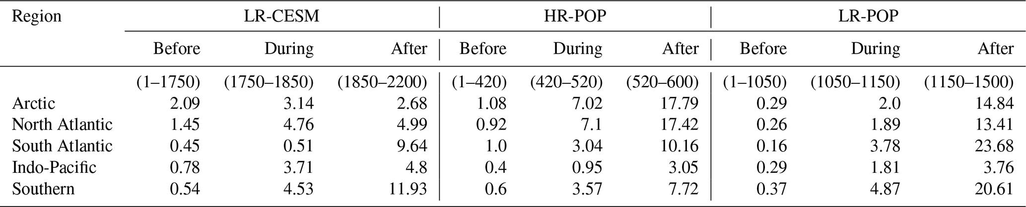
Table A2 DSL sensitivities under varying hosing and DSL differences for fixed hosing in the LR-CESM. For DSL sensitivities, the DSL differences are determined between model years 2200–3200 ($\mathrm{\Delta }{F}_H=-\mathrm{0.3}$ Sv, AMOC strength ≈0 Sv) in the backward QE LR-CESM. The DSL differences are determined between the “AMOC off” state and “AMOC on” state for $\stackrel{\mathrm{‾}}{F_H}=\mathrm{0.18}$ Sv and $\stackrel{\mathrm{‾}}{F_H}=\mathrm{0.45}$ Sv.

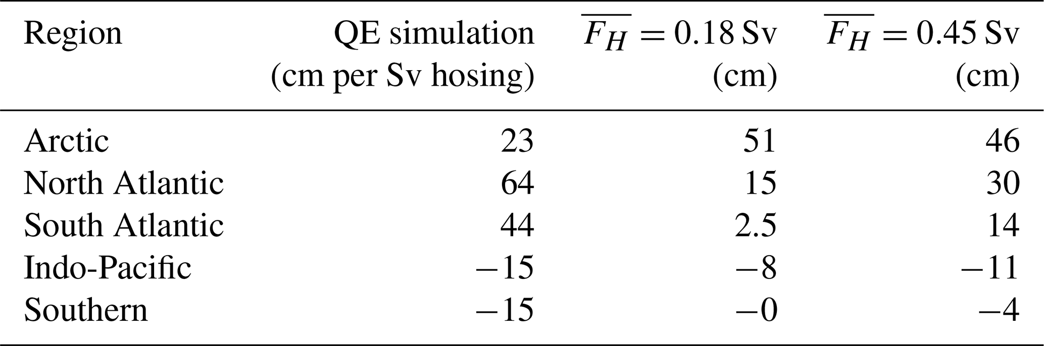
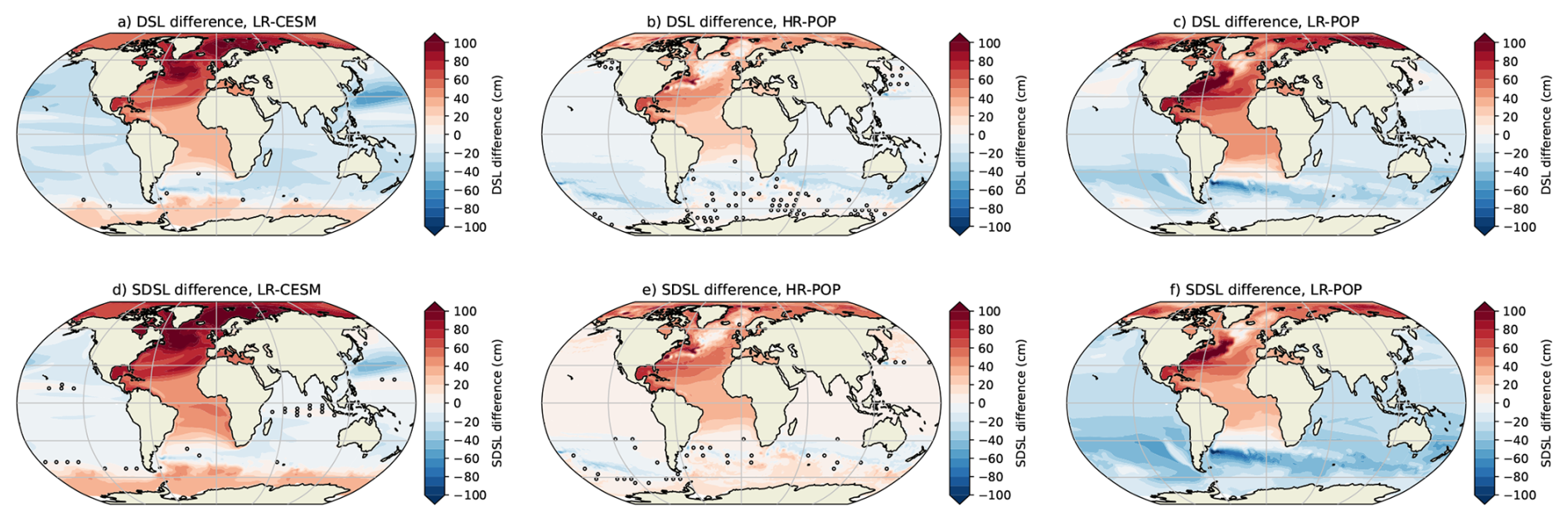
Figure A1 (a–c) Dynamic sea-level (DSL) differences between the last 50 model years and first 50 model years of the (forward QE) LR-CESM, HR-POP and LR-POP. (d–f) Sterodynamic sea-level (SDSL) differences between the last 50 model years and first 50 model years of the (forward QE) LR-CESM, HR-POP and LR-POP. In all panels, the markers indicate non-significant (p≥0.05) differences.

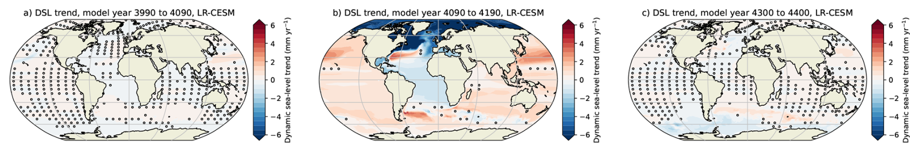
Figure A2 DSL trends over 101-year windows for the backward quasi-equilbirium LR-CESM, where markers indicate non-significant (p≥0.05) DSL trends. The 101-year windows are (a) before the AMOC recovery, (b) during the AMOC recovery, and (c) after the AMOC recovery (the last 101 model years).

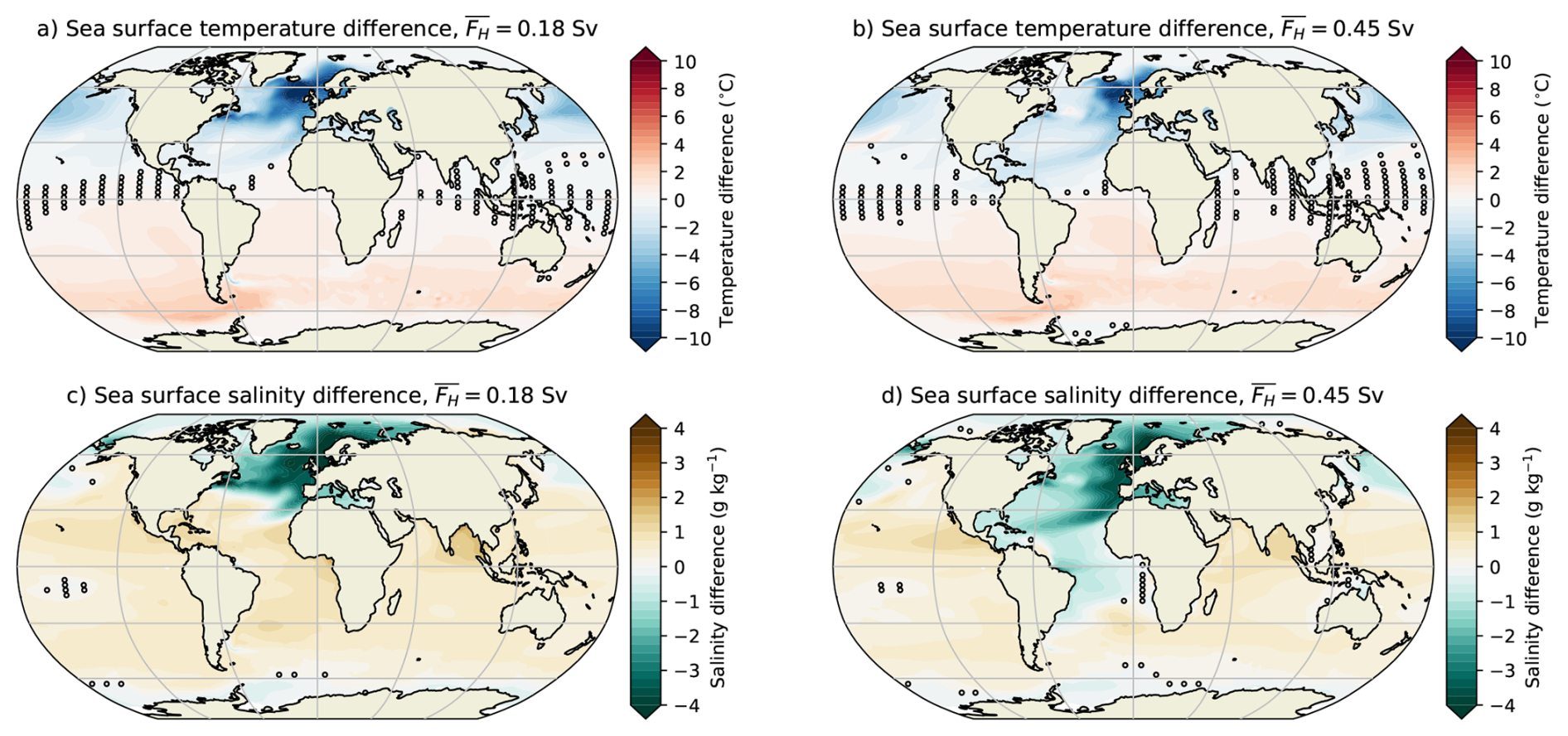
Figure A3 (a, b) Sea surface temperature differences between the statistical equilibria for $\stackrel{\mathrm{‾}}{F_H}=\mathrm{0.18}$ Sv and $\stackrel{\mathrm{‾}}{F_H}=\mathrm{0.45}$ Sv, displayed as the “AMOC off” state minus the “AMOC on” state. (c, d) Sea surface salinity differences between the statistical equilibria for $\stackrel{\mathrm{‾}}{F_H}=\mathrm{0.18}$ Sv and $\stackrel{\mathrm{‾}}{F_H}=\mathrm{0.45}$ Sv, displayed as the “AMOC off” state minus the “AMOC on” state. The markers indicate non-significant (p≥0.05) differences.

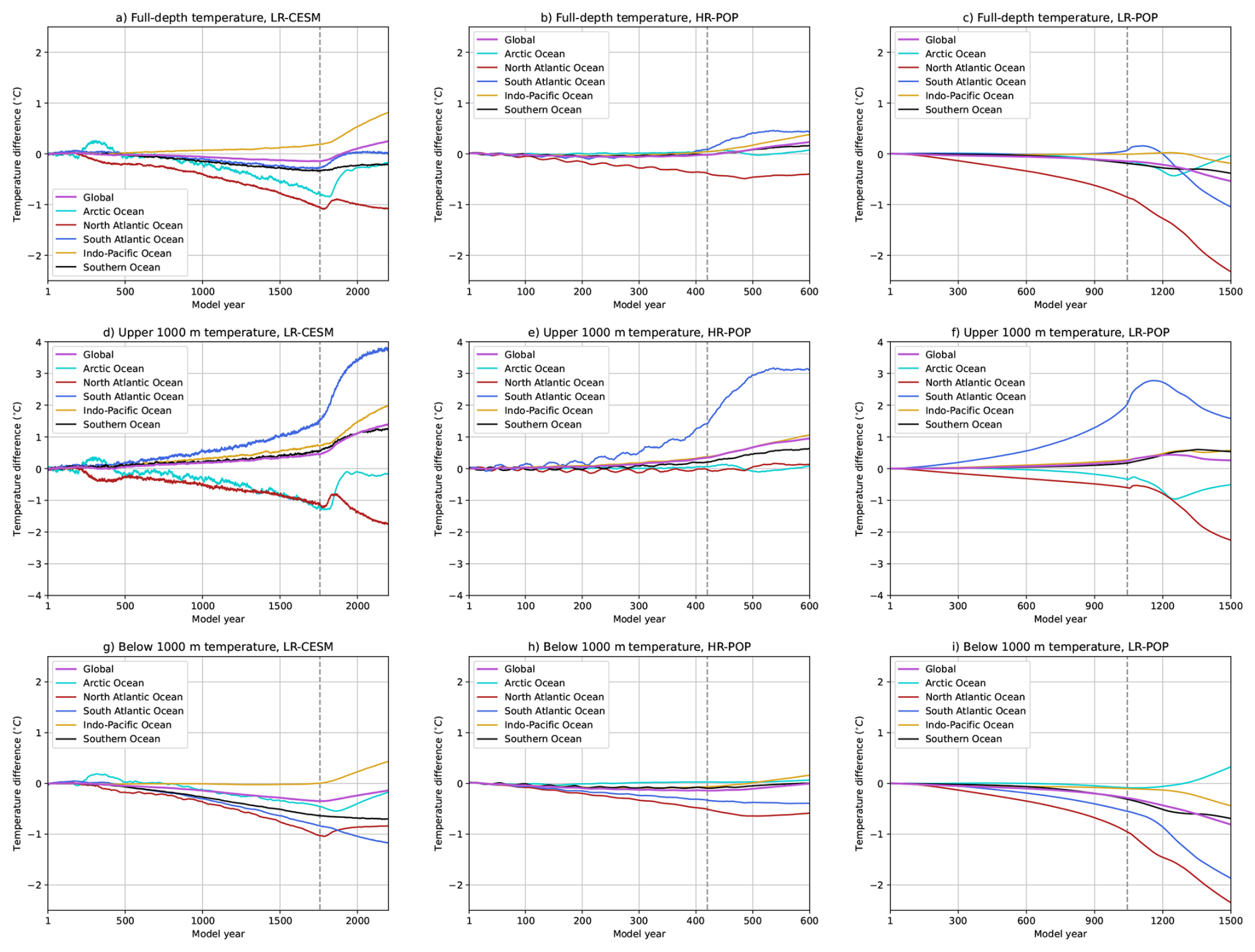
Figure A4 Volume-averaged oceanic temperature responses for the five different regions and global mean for the LR-CESM (left), HR-POP (middle) and LR-POP (right). The full-depth temperatures (upper row) are decomposed into an upper 1000 m contribution (middle row) and below 1000 m contribution (lower row). All time series are displayed as differences compared to the first 50 model years and are smoothed through a 25-running mean to reduce the variability. The dashed gray line indicates the onset of the AMOC collapse.

Figure A5 Similar to Fig. A4, but now for the salinity.

Figure A6 Similar to Fig. 10b, c, but now for the backward QE simulation (model years 2200–4400, right to left). The dashed gray line indicates the onset of the AMOC recovery.