Can the boundary profiles at 26° N be used to extract buoyancy-forced Atlantic Meridional Overturning Circulation signals?

The temporal variability of the Atlantic Meridional Overturning Circulation (AMOC) is driven both by direct wind stresses and by the buoyancy-driven formation of North Atlantic Deep Water over the Labrador Sea and Nordic Seas. In many models, low-frequency density variability down the western boundary of the Atlantic basin is linked to changes in the buoyancy forcing over the Atlantic subpolar gyre (SPG) region, and this is found to explain part of the geostrophic AMOC variability at 26^∘ N. In this study, using different experiments with an ocean general circulation model (OGCM), we develop statistical methods to identify characteristic vertical density profiles at 26^∘ N at the western and eastern boundaries, which relate to the buoyancy-forced AMOC. We show that density anomalies due to anomalous buoyancy forcing over the SPG propagate equatorward along the western Atlantic boundary (through 26^∘ N), eastward along the Equator, and then poleward up the eastern Atlantic boundary. The timing of the density anomalies appearing at the western and eastern boundaries at 26^∘ N reveals ∼ 2–3-year lags between boundaries along deeper levels (2600–3000 m). Record lengths of more than 26 years are required at the western boundary (WB) to allow the buoyancy-forced signals to appear as the dominant empirical orthogonal function (EOF) mode. Results suggest that the depth structure of the signals and the lagged covariances between the boundaries at 26^∘ N may both provide useful information for detecting propagating signals of high-latitude origin in more complex models and potentially in the observational RAPID (Rapid Climate Change programme) array. However, time filtering may be needed, together with the continuation of the RAPID programme, in order to extend the time period.

1 Introduction

The Atlantic Meridional Overturning Circulation (AMOC) plays a key role in controlling the Earth's energy budget. It transports warm water to the north, overlaying a return flow southward of colder and denser water (Cunningham et al., 2007). Due to its large net heat transport, low-frequency variability in this circulation can have an important impact on Atlantic sea surface temperatures (SSTs) and therefore on the wider climate (Knight et al., 2005; Sutton and Dong, 2012). Decadal prediction systems have shown that the upper ocean temperatures over the subpolar gyre can be predicted due to the leading role of the ocean heat transport (Robson et al., 2012, 2017; Hermanson et al., 2014). In order to make these decadal predictions, it is essential that we ensure the best ocean initial conditions are available with a well reproduced AMOC.

RAPID (Rapid Climate Change programme) has been monitoring AMOC and boundary densities at 26^∘ N since 2004 (Cunningham et al., 2007; McCarthy et al., 2015). The observational record so far has revealed a large range of AMOC variability on different timescales: from high-frequency variability (Balan Sarojini et al., 2011) to large anomalies persisting at inter-annual timescales (Blake et al., 2015; Roberts et al., 2013) or decadal trends (Smeed et al., 2014; Jackson et al., 2016). Using different methods, several studies have investigated the observed weakening (since 2005) of the AMOC and have related the trends to earlier high-latitude density changes (Jackson et al., 2016; Robson et al., 2014, 2016).

The AMOC circulation is driven both by direct wind stresses and by the buoyancy-driven formation of North Atlantic Deep Water (NADW) over the Labrador Sea and Nordic Seas. Theories of the response of the AMOC and the ocean gyres to wind stress or buoyancy input rely on energy being transmitted through the ocean by planetary Rossby waves or along the ocean margins by boundary waves (Johnson and Marshall, 2002; Hirschi et al., 2007; Hodson and Sutton, 2012; Jackson et al., 2016). In particular, changes in the NADW may produce a chain of events in the North Atlantic on a range of timescales from months to decades. The adjustment has been studied in an extensive literature. Some model studies (Kawase, 1987; Huang et al., 2000; Johnson and Marshall, 2002; Getzlaff et al., 2005; Marshall and Johnson, 2013) suggest that AMOC anomalies propagate with boundary Kelvin wave speeds resulting in a very short lead time (of the order of a few months) between subpolar and subtropical AMOC changes. Roussenov et al. (2008) suggested that this boundary propagation may also involve higher-mode Kelvin and topographic Rossby waves, leading to longer propagation times (of the order of years). The advection of the NADW outflow also moves down the western boundary more slowly in the Deep Western Boundary Current (DWBC), although Lagrangian float observations show that a large fraction of this NADW moves away from the boundary and enters the ocean interior near the Flemish Cap and the Grand Banks (Bower et al., 2009). Using a coupled climate model, Zhang (2010) and Zhang et al. (2011) showed AMOC variations associated with NADW formation propagating more in line with the advection speed, with much longer lead times (several years) between subpolar and subtropical AMOC variations. Getzlaff et al. (2005) have shown that the high-latitude adjustment to AMOC anomalies can result from a superposition of a fast wave response and a slower advective signal in ocean model experiments with different resolutions. Interestingly, the speed of propagation along boundaries of the density or velocity anomalies related to AMOC changes is found to be model-resolution dependent (Getzlaff et al., 2005; Hodson and Sutton, 2012). These propagating density anomalies will also affect the geostrophic AMOC variability at 26^∘ N.

Model simulations clearly show a large range of mechanisms leading to AMOC variability at the latitude 26^∘ N (Hirschi et al., 2007; Biastoch et al., 2008; Cabanes et al., 2008; Duchez et al., 2014; Polo et al., 2014; Pillar et al., 2016). Buoyancy forcing generally operates from inter-annual to decadal timescales, while the wind forcing mostly acts from intra-seasonal to inter-annual timescales (Cabanes et al., 2008; Kanzow et al., 2010; Duchez et al., 2014; Polo et al., 2014; Pillar et al., 2016). Using an adjoint ocean general circulation model (OGCM), Pillar et al. (2016) have found that inter-annual to inter-decadal AMOC variability of ∼5 Sv (sverdrup) amplitude can be excited by heat fluxes in the subpolar North Atlantic, with freshwater fluxes playing a more minor role. Originating from higher latitudes, the western boundary (WB) density anomalies explain most of the variance in the zonal density gradients (and hence geostrophic transports) at 26^∘ N, especially at decadal timescales (Hirschi et al., 2007; Polo et al., 2014). The eastern boundary (EB) explains only a small part of the inter-annual variability in zonal density gradients in the upper 1500 m, and this is mostly due to local wind forcing (Polo et al., 2014).

Despite the many model studies showing boundary wave connections between the Labrador Sea and lower latitudes, as well as their importance for the AMOC, less work has been done on the vertical structure of these anomalies. Yet, it is the vertical density structure at 26^∘ N that is primarily measured by the RAPID array. We now benefit from more than 10 years of boundary density records at 26^∘ N; therefore, we can consider how best to use the vertical structure in these data to study the lower-frequency variability. If low-frequency signals can be identified from the vertical structure, then this would help us to assimilate the most important signals that need to be reproduced in climate forecast models. This poses the question we address in this paper: can we extract the buoyancy-forced signals from vertical density profiles, such as those sampled at 26^∘ N?

An earlier attempt to extract buoyancy signals at 26^∘ N was made by Polo et al. (2014, hereafter PA14) using a NEMO (Nucleus for European Modelling of the Ocean) 1^∘ OGCM forced with full European Centre for Medium-Range Weather Forecasts (ECMWF) reanalysis meteorology from 1958 to 2010 (denoted as the CTRL experiment hereafter). This CTRL experiment was compared to runs using only inter-annual wind or buoyancy forcing, allowing for separation of buoyancy from wind-forced variations in the AMOC. PA14 found that the buoyancy-forced AMOC anomalies at 26^∘ N could be related to changes in deep water formation over the Labrador Sea some years before. Although they showed a coherent WB vertical signal at 26^∘ N, they were not successful in isolating the buoyancy-forced signal in the CTRL experiment, due to the confounding influence of the wind-forced variability. They did not look in detail at the propagation or how the vertical structure associated with the buoyancy-forced anomalies develops. In the present work, we extend the work by PA14 by (i) developing statistical means of isolating the buoyancy-forced AMOC variability from the full variability in the CTRL using the density profiles at 26^∘ N, (ii) analysing the propagation of the buoyancy-forced signals from the Labrador Sea down to the subtropics and (iii) developing statistical covariance relationships linking the AMOC to the Labrador Sea that might potentially be used in a data assimilation context to modify the low-frequency AMOC variability. The diagnostics developed are also tested on RAPID observations and on output from the state-of-the-art coupled model HadGEM3-GC2 (Williams et al., 2015), which has a 1∕4^∘ NEMO global ocean.

In this paper, Sect. 2 presents the methodology used to analyse AMOC variability and its sources in several runs of the NEMO model (1^∘ × 1^∘ horizontal resolution) driven by different components of ECMWF atmospheric forcing from 1960 to 2012, as in PA14, but now including some validation of the boundary density variability in the CTRL run against the RAPID observations. Sections 3 and 4 describe the modes of the 26^∘ N density profile variability in the model and the associated propagation occurring upstream and downstream, respectively. Section 5 describes a statistical analysis of boundary densities in the RAPID observations and compares these modes with the NEMO experiments. Section 6 discusses density variability in the coupled experiments (GC2) in comparison to the lower-resolution results. Section 7 discusses the results and limitations of the interpretations. Finally, Sect. 8 summarises the main conclusions.

2 Methodology

This section describes the model experiments and statistical methods used to understand the boundary density variability and its relation to the AMOC variability.

2.1 Forced experiments

The forced ocean-only model (hereafter NEMO1) is based on NEMO V3.0; it uses the tripolar ORCA (Madec et al., 1998) grid in a global configuration with 1^∘ × 1^∘ horizontal resolution and a tropical meridional refinement to 1∕3^∘. The model has 42 vertical levels with thicknesses ranging from 10 m at the surface to 250 m at the ocean bottom. Initial conditions are taken from the second iteration of a 50-year cyclic model spin-up, with each cycle spanning the period 1958–2009 (Balmaseda et al., 2013). The model is forced with daily atmospheric fluxes as boundary conditions taken from the ECMWF reanalysis ERA-40; (Uppala et al., 2005) from 1958 to 1978 and the interim ECMWF reanalysis (ERA-Interim; Dee et al., 2011) from 1979 to 2009.

The control experiment (CTRL) is forced with time-varying daily surface heat, freshwater and momentum fluxes for the period 1958–2009. The sea surface temperature (SST) is weakly relaxed to daily values with a relaxation timescale of ∼1 month, while the sea surface salinity (SSS) is restored to climatological SSS with a timescale of 1 year. There is no ice model; instead, wherever the sea ice concentration in the observations exceeds 55 %, the model SSTs are nudged more strongly (1 d timescale) to the freezing point (−1.88 ^∘C). The restoration to SSS and SST is stronger under sea ice (30 and 1 d, respectively).

Following the work by PA14, we also have a set of simulations where the momentum and buoyancy forcing are decoupled from one another. In the experiment referred to as BUOY, the momentum flux is taken from the ERA-Interim 1989–2009 seasonal climatology, while the buoyancy forcing (heat, freshwater flux and SST) is still inter-annually varying. In the experiment referred to as WIND, the momentum flux is fully varying, but the buoyancy forcing is from the same seasonal climatology. These experiments allow us to identify and distinguish the AMOC signals and processes associated with buoyancy and wind forcing to the extent that they are independent. We use the BUOY experiment as reference for the buoyancy-forced-only signals and the CTRL experiment as the “truth”, which includes both buoyancy and wind forcings, as well as the interaction between them. Where appropriate, we also include the WIND experiment and SUM (as the sum of anomalies from BUOY and WIND). Results are discussed in Sects. 3 and 4.

2.2 Coupled experiment

We also analyse 120 years of monthly-mean data from a control run of the high-resolution coupled ocean–atmosphere model HadGEM3-GC2 (hereafter GC2; Williams et al., 2015). The ocean component is NEMO v3.4 with the ORCA025 tripolar grid configuration, using Met Office parameters for “Global Ocean 5.0” (GO5.0; Megann et al., 2014), with the CICE (Bitz and Lipscomb, 1999) sea ice model. The atmosphere component is GA 6.0 of the Met Office Unified Model (UM; Walters et al., 2011) at a resolution of N216 (∼60 km in mid-latitudes) and 85 levels. This model was used in the Met Office seasonal and decadal prediction systems (GloSea5 and DePreSys3, respectively). The model has been used to study the North Atlantic variability and its predictability (Menary et al., 2015; Williams et al., 2015; Ortega et al., 2017; Robson et al., 2016). Results are shown in Sect. 6.

2.3 Model evaluation

We use the RAPID array (McCarthy et al., 2015; Smeed et al., 2017) to evaluate the boundary densities in the model. We use the merged profiles at the western boundary (26.52^∘ N, 76.74^∘ W) and eastern boundary (26.99^∘ N, 16.23^∘ W) for the period April 2004 to December 2009.

Figure 1 shows the profiles of temperature, practical salinity and density at the boundaries for the RAPID and CTRL experiments. The main differences occur at the EB in the upper 1000 m, especially in temperature and salinity (Fig. 1a, b), probably due to a bias in the location of the Mediterranean Water. Beneath 2000 m, the variables in CTRL and RAPID are very similar.

Figure 1 Temperature, salinity and density profiles at 26^∘ N. (a) Temperature profiles (in ^∘C) at 26^∘ N for western boundary (WB, blue line) and eastern boundary (EB, green line) for the CTRL experiment (dashed line) and the RAPID data (solid line) for the period 2004–2009. (b) Same as (a) but for the salinity profiles. (c) Same as (a) but for the density profiles (in kg m⁻³).

NEMO1 and GC2 are both able to capture important aspects of the observed boundary density profiles such as the mean vertical density gradients (N², Fig. S1a in the Supplement). On the WB the profiles are similar between 1500 and 4500 m, but the model stratification is stronger between 300 and 700 m. The EB profiles are similar at all levels below 500 m (Fig. S1a). However, the NEMO1 model underestimates the density variance at all levels, especially at the WB, while GC2 has a more realistic variance on the WB at depth (Fig. S1b).

The AMOC at 26^∘ N in NEMO1 has a time mean (12 Sv) and maximum (18 Sv) at a depth of 1000 m in the CTRL experiment. The mean AMOC is higher in the BUOY experiment by ∼2 Sv. The AMOC measured at 1000 m has a prominent trend in the BUOY experiment (+3.2 Sv in 52 years), but the trend is not significant for the CTRL (−0.2 Sv in 52 years). The AMOC seasonal cycle (not shown) in the CTRL presents a maximum in boreal winter with a secondary peak in boreal summer, which is also reproduced in the BUOY experiment. The annual cycle defined as the difference between the maximum (in boreal winter) and the minimum (in boreal spring) is 3.9 and 4.9 Sv for the CTRL and BUOY experiments, respectively. After removing the linear trend, the standard deviation of both experiments is similar: 2.28 and 1.92 Sv for CTRL and BUOY, respectively (see also Fig. S2 for the AMOC distributions). The AMOC at 26^∘ N in the RAPID observations presents a mean and maximum of 17 and 31 Sv, respectively, from 2004 to 2014, with monthly standard deviation of 4.35 Sv, which is double the standard deviation for the CTRL experiment. Trends have been reported for RAPID data of −0.6 Sv yr⁻¹ (Smeed et al., 2014, 2018), which could be part of a longer variation cycle (Smeed et al., 2018; Jackson et al., 2016). Results from the modes of variability at the western boundary density profile are shown in Sect. 5.

2.4 Statistical analysis

Model experiments are first sampled at the western and eastern Atlantic boundaries at 26^∘ N to simulate the monthly-mean density profiles from the RAPID array. Empirical orthogonal function (EOF) analysis of these density profiles is used to obtain vertical modes of density variability and related time series of principal components (PCs), which together represent the largest fractions of the total variance (Bretherton et al., 1992).

Before calculating the EOFs, the data are processed to remove the seasonal cycle and linear trends. Unlike in PA14, density anomalies are weighted by the thickness of each layer to ensure that all points are appropriately represented for the total density variability. The EOF analysis is computed for the individual boundaries – western boundary (WB) and eastern boundary (EB) – and also for the combined anomalies at both boundaries. Finally, we have explored the combined EOFs by lagging the eastern boundary variability in order to understand related signals from both boundaries.

The PC time series is normalised (the units are standardised anomalies), and the associated EOF is represented as the regression map of the density anomalies (in kg m⁻³) superimposed onto the PC time series. Therefore, the EOF pattern has density units (density anomalies by 1 standard deviation of the PC). The PC is calculated from monthly data of the density profiles. The PC from 800 m is calculated using only the information from 800 m downwards. However, the resulting EOF pattern, by computing the regression map, can have a density signal shallower than 800 m.

Regression analysis of the PC time series on other fields (e.g. 3D density) allows us to detect spatial patterns and depth structures of the propagating modes associated with the EOFs at 26^∘ N. We show regression and the correlation coefficients where they are statistically significant at the 95 % confidence level, according to a Student's t test for the effective number of degrees of freedom (Metz, 1991).

2.5 Spectral analysis

In order to remove the high frequencies in the time series in Sect. 3, we have used a 1-year running-mean filter. This filtered time series is obtained by taking the average of a data subset (13 months) which is centred in a monthly time step (von Storch and Zwiers, 1999).

Spectral analysis is used to decompose the time series to show signals that lie within different frequency bands. The analysis is performed in order to identify the frequencies involved in the propagation of density anomalies at different depths. Power spectra of the time series are obtained using the multi-taper method, which provides more degrees of freedom and therefore more significance (Thomson, 1982). The power spectra are tested against the hypothesis that the signals are generated by a first-order autoregressive process, AR(1), with the same timescale as the original, yielding a red noise spectrum, and the 95 % confidence limit for the rejection of the red noise hypothesis is applied. Additionally, when we have a large internal variability, we use the decomposition in order to filter some of the time series using a Lanczos (1956) filter. This is done in particular for the control GC2 simulation.

We have used the Radon transform (RT) function (Dean, 1983) in order to estimate the phase speed of propagation of density anomalies. The angle of the maximum RT standard deviation determines the propagation phase speed. We calculate the RT every 0.1^∘. The phase speed averaged for the Hovmöller diagrams has been estimated at the 3000 m level for the CTRL and BUOY experiments.

3 Modes of vertical density variability at the 26^∘ N boundaries

3.1 Linearity of AMOC and the boundary density signals in the NEMO1 model

The forced ocean model experiments enable us to isolate the boundary density variability associated with buoyancy forcing, i.e. from the BUOY experiment, as noted by PA14. We focus here on developing the vertical density fingerprint of this signal and using it to identify the buoyancy-forced AMOC signal as it appears in the CTRL run.

Figure 2a shows the monthly AMOC (the total AMOC minus Ekman component) variability, defined as the integral of the meridional transport at 26^∘ N down to 1028 m, for both the CTRL and BUOY experiments (as in Fig. 1a in PA14). There is a prominent decadal signal in both CTRL and BUOY with peaks in 1975, 1985 and 1995, although CTRL also shows additional monthly and inter-annual variability. Similar decadal signals of AMOC variability are reproduced by reanalysis products (Wang et al., 2010; Karspeck et al., 2017). The monthly-mean time series correlate at 0.43, but the correlation rises to 0.62 when using a 1-year running-mean filter (Fig. 2b). Wind-forced inter-annual variability explains most of the remaining differences; when the 1-year smoothed AMOC anomalies from BUOY and WIND are summed the correlation with CTRL rises to 0.86 (SUM in Fig. 2b).

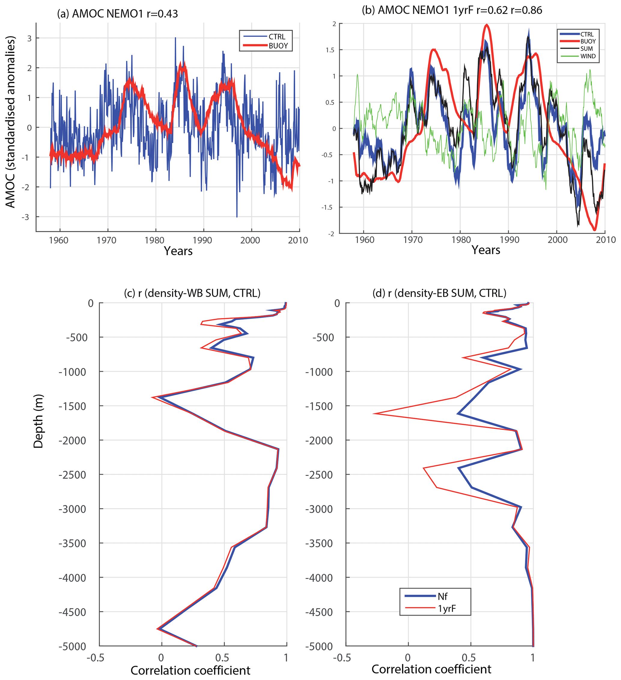
Figure 2 AMOC and linearity of the forcings for the density profiles at the boundaries. (a) Geostrophic AMOC defined at 26^∘ N and 1100 m for the CTRL (blue line) and BUOY (red line) experiments. In the title, the correlation between both time series is detailed. (b) Same as (a) but the time series have been smoothed with a 1-year running-mean filter. Black line refers to AMOC for the SUM (BUOY + WIND). Green line is the filtered AMOC time series for the WIND experiment. In the titles, correlations between blue and red and between blue and black lines are detailed. (c) Correlation coefficient between profiles of density anomalies at the WB for the CTRL experiment and the SUM. Blue line refers to anomalies without time filter; red line refers to anomalies that have been smoothed with a 1-year running-mean filter. (d) Same as (c) but for the EB.

Most of the boundary density variability is also recreated in BUOY and WIND. The correlations between boundary density anomalies in CTRL and SUM are shown as a function of depth in Fig. 2c–d. For the WB, most of the CTRL variability is reproduced by SUM from 1800 to 4000 m (Figs. 2c and S3). For the EB, SUM explains most of the variability seen in the CTRL experiment at all depths (Figs. 2d and S3). A 1-year low-pass filtering does not influence the correlations for the WB, although for the EB filtering reduces the correlation at some depths. We now relate this density variability with the AMOC signals in Fig. 2a and b.

3.2 EOFs of boundary density profiles

Figure 3 shows the principal component time series of the first EOF computed using monthly density profiles on the western and eastern boundary at 26^∘ N for the CTRL (blue) and BUOY (red) experiments. As density profiles near the surface contain significant noise, we calculate the PCs for both full-depth profiles (f_0 m, Fig. 3a–b) and only from 800 m downwards (f_800 m, Fig. 3c–d). The full-depth PCs in Fig. 3a both show substantial high-frequency noise, and the CTRL time series does not correlate well with AMOC variability from Fig. 2a. However, when only retaining densities below 800 m, in Fig. 3c, the BUOY and CTRL PCs closely match each other (r=0.80), and both now correlate with the AMOC time series in Fig. 2a (r=0.33 and r=0.88 for CTRL and BUOY, respectively). These f_800 m EOFs also explain more of the deeper density variance. Note that adding a 1-year filter to the PC-CTRL time series increases the correlations with the CTRL AMOC variability to 0.47 (Fig. 3c). However, for the BUOY experiment the temporal filter has little impact on the correlation between PC and AMOC time series (0.89).

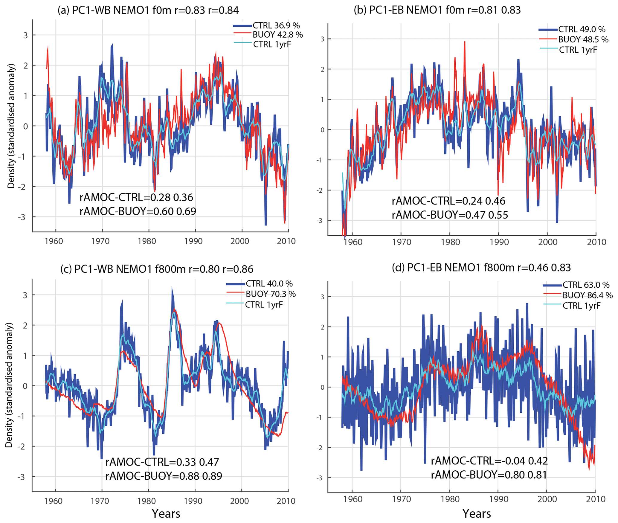
Figure 3 AMOC at 26^∘ N and individual EOF of density profiles at the 26^∘ N boundaries: sensitivity to depth truncation. (a) Time series associated with the leading mode of density variability of the water column at the WB for the CTRL (blue line) and BUOY experiments (red line), using the full water column. Cyan line corresponds to the time series of the CTRL smoothed with a 1-year running-mean filter. In the title, correlations between blue and red and between blue and cyan lines are detailed. (b) Same as (a) but for the EB. (c–d) Same as (a)–(b) but considering the EOF analysis with profiles from 800 m downwards. Time series are dimensionless, and the percentage of explained variance is seen inset. Also, on the bottom, the correlations between PCs and the AMOC are detailed for time series without filter and smoothed with a 1-year running mean filter.

Figure 3b and d show the corresponding eastern boundary density EOF time series for full depth and below 800 m variability. The full-depth PC is rather different to that on the western boundary and also to the AMOC variability itself. However, when only the deep variability is retained, the inter-annual variability in BUOY is more similar to the western boundary buoyancy-driven variability. In CTRL there is still considerable high-frequency wind-generated variability in the deep PC; however, when a 1-year filter is introduced, the buoyancy-forced AMOC-related signal becomes clearly visible on the eastern boundary, and the correlation with the AMOC rises to 0.42 (Fig. 3d). All correlations are summarised in Table 1.

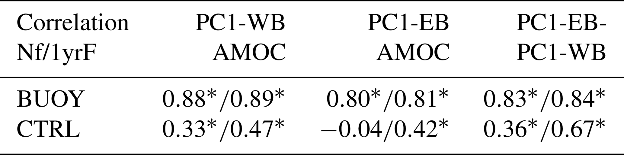
Table 1 Correlations between PCs f_800 m and AMOC time series in NEMO1 are shown. Correlations between the geostrophic AMOC and the PCs at the boundaries for the CTRL and BUOY experiments are also shown. Significant correlations are highlighted with a star (^∗) based on a t test at 95 % confidence level and after calculating the number of effective degrees of freedom. Time series with no filter (Nf) and with 1-year running mean filter (1yF) are shown in the same cell separated by a slash.

In order to understand the usefulness of truncating the density profiles for the EOFs, Fig. 4a–b summarise correlations between leading PCs at the boundaries and AMOC time series in the CTRL experiment by increasing the truncation level for the density profiles. For the WB, maximum correlation is found simultaneously at all truncations, especially for deeper levels (Fig. 4a). In contrast, for the EB simultaneous correlations are always low even with a 1-year filter, but correlations increase greatly when a lag is applied to the AMOC (Fig. 4b). Correlations still require a 1-year filter to remove noise, but now there is a peak at 0.7 with a lag of around 2–3 years, with the more deeply truncated signals also showing longer lags. Similar lag-increased EB correlations are found for the BUOY experiment (not shown). The nature of this lag in the EB-AMOC correlation is related to signal propagation between boundaries and will be discussed in the next section.

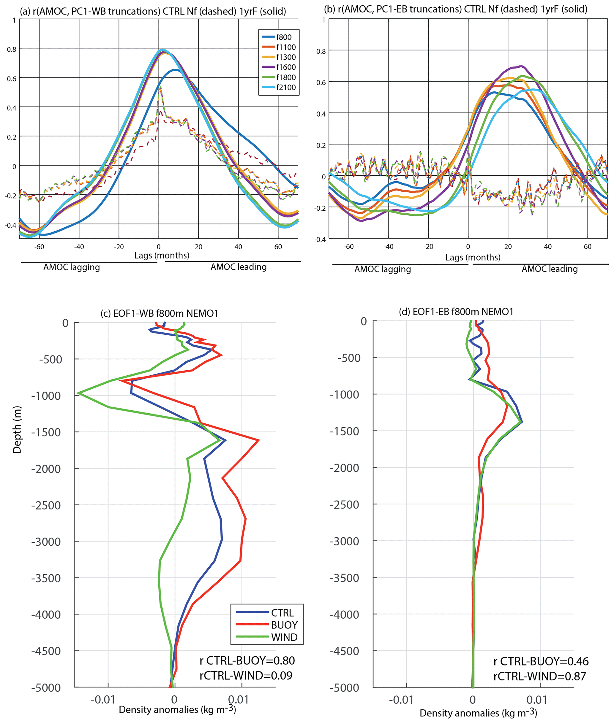
Figure 4 Individual EOFs of density profiles at the 26^∘ N boundaries from 800 m are shown. (a) Lead–lag correlations between AMOC and PC1-WB at different truncations are shown (represented with different colours). Positive (negative) values over the x axis represent the AMOC leading (lagging) PC1-WB. A 1-year running-mean filter (solid line) and no filter (dashed line) are applied to the time series for the CTRL experiment. (b) Same as (a) but for the correlations between AMOC and PC1-EB. (c) Profile of density anomalies (in kg m⁻³) associated with the leading mode of density variability of the water column from 800 m downwards at WB for the CTRL (blue line), BUOY (red line) and WIND (green line) experiments. Associated time series are in Fig. 3c except for the WIND experiment. (d) Same as (c) but for the EB; associated time series are in Fig. 3d except for the WIND experiment. Correlation coefficients between time series of the PCs for CTRL with BUOY and WIND are detailed.

Figure 4c–d show the vertical structure of density anomalies associated with the leading EOF modes for both boundaries using the 800 m depth truncation and monthly-mean data for the three experiments (CTRL, BUOY and WIND). The leading EOFs are very similar between CTRL and BUOY on the WB, with maxima between 1200 and 4000 m. Note that in PA14 Fig. 3b, their PC-WB in the CTRL experiment with only 500 m depth truncation was substantially different and was mainly wind driven. The WIND experiment has much less variability at greater depths, and the PC is uncorrelated with the PC-WB from CTRL (r=0.09, Fig. 4c). Therefore, on the WB, Figs. 3c and 4c show that the EOF analysis successfully extracts the buoyancy-forced signal related to the AMOC in the CTRL.

On the EB the leading EOFs, even below 800 m, show more correspondence between CTRL and WIND (Fig. 4d, with PC correlations r=0.87). This explains why further filtering and the application of a lag to the PC time series in Figs. 3d and 4b is needed to extract the weaker buoyancy-forced AMOC-related signal on the EB. The relationship between these buoyancy-driven density variations at both boundaries is now explored further.

3.3 Relationship between boundaries

Figure 5a shows lead–lag correlations between the WB leading PCs (computed from 800 m depth) and the EB at different depth truncations in the CTRL experiment. Dashed (solid) lines indicate PCs without (with) the application of a 1-year running-mean filter. For truncations deeper than 1600 m, the highest correlation is found when the EB is lagged up to 30 months (Fig. 5a), revealing longer links between boundaries for deeper levels. However, this lag is much less clear when shallower depths are retained, and substantial WB–EB density correlations start to be seen with a lag of 0 (unlike in Fig. 4b). Even in the BUOY experiment, only when the EB EOFs are truncated to below 1600 m is a strong lag clearly seen between the boundaries, again reaching up to 30 months for the deepest signals (Fig. 5b).

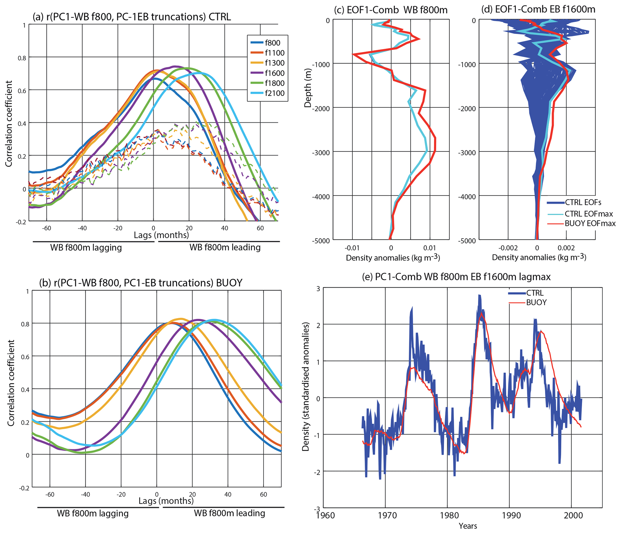
Figure 5 Relationship between boundaries and the combined EOF. (a) Lead–lag correlations between PC1-WB from 800 m and PC1-EB at different truncations (represented with different colours). Positive (negative) values over x axis represents the PC1-WB leading (lagging) the PC1-EB. A 1-year running-mean filter (solid line) and no filter (dashed line) are applied to the time series for the CTRL experiment. (b) Same as (a) but for the BUOY experiment, and only the 1-year running-mean filter is plotted. Panels (c)–(d) are the EOFs as a result of combining the density profile at the WB (from 800 m) at lag 0 and the EB (from 1600 m) at different lags. The CTRL experiment is plotted in blue and the cyan line corresponds to the EOF at the lag in which the explained fraction of variance is maximum (EOFmax). The latter equivalent EOFmax profile for the BUOY experiment is plotted in red. (e) The associated time series of EOFmax for the CTRL (blue) and BUOY (red) experiments.

In order to reduce upper-level noise at the EB and to bring out the deep density signal connecting the boundaries more clearly, we compute the combined EOF while truncating the EB to below 1600 m, which shows a maximum in the WB–EB correlations for CTRL (Fig. 5a). The new combined EOF shows similar WB structure for all lags (Fig. 5c) with a deeper signal around 2000 m on the EB (Fig. 5d). Figure 5e shows the time series, which is very similar to the PC1-WB in Fig. 3c. The new combined EOF explains more density variance in CTRL (43 % compared to 40 % explained by PC1-WB) and a slightly longer lag between WB and EB (18 months in CTRL and 25 months in BUOY, not shown).

We conclude that the deep densities on the EB contain a very clear signal of the buoyancy-forced AMOC variability but that this signal plays no detectable role in the direct (lag 0) control of the AMOC. The EB lag signal can also be seen in relation to the PC-WB density, although the signal is less clearly lagged, probably reflecting the noise still present in the upper-layer densities on the WB.

The WB clearly contains the core density information on the buoyancy-forced AMOC changes at low frequencies. Using PC1-WB, we will now identify the propagating density signal connecting the boundaries (Sect. 4) and search for similar signals in the RAPID data (Sect. 5) and in the higher-resolution GC2 model (Sect. 6).

4 Propagation of the buoyancy-driven signals

Motivated by the lagged signal at the EB, we analyse the (i) spatial coherence of the anomalies at deeper levels (∼ 3000 m) and (ii) the propagation fingerprints of the connecting signals.

4.1 Spatial regression patterns

Figure 6 shows the spatial density anomalies averaged over 2700–3000 m, regressed onto the PC1-WB for the CTRL and BUOY experiments, at different lags. At these deep levels, the regression patterns in CTRL (Fig. 6a–c) and BUOY (Fig. 6d–f) are very similar to each other. This agreement suggests that although the magnitude of the regressions is stronger in BUOY, we are identifying the same signal in both experiments. The density signal in the Labrador Sea appears from a lag of −30 (Fig. 6a, d) and intensifies and propagates down the WB to the Equator (Fig. 6b, e) and then across the Equator and poleward at the EB (Fig. 6c, f).

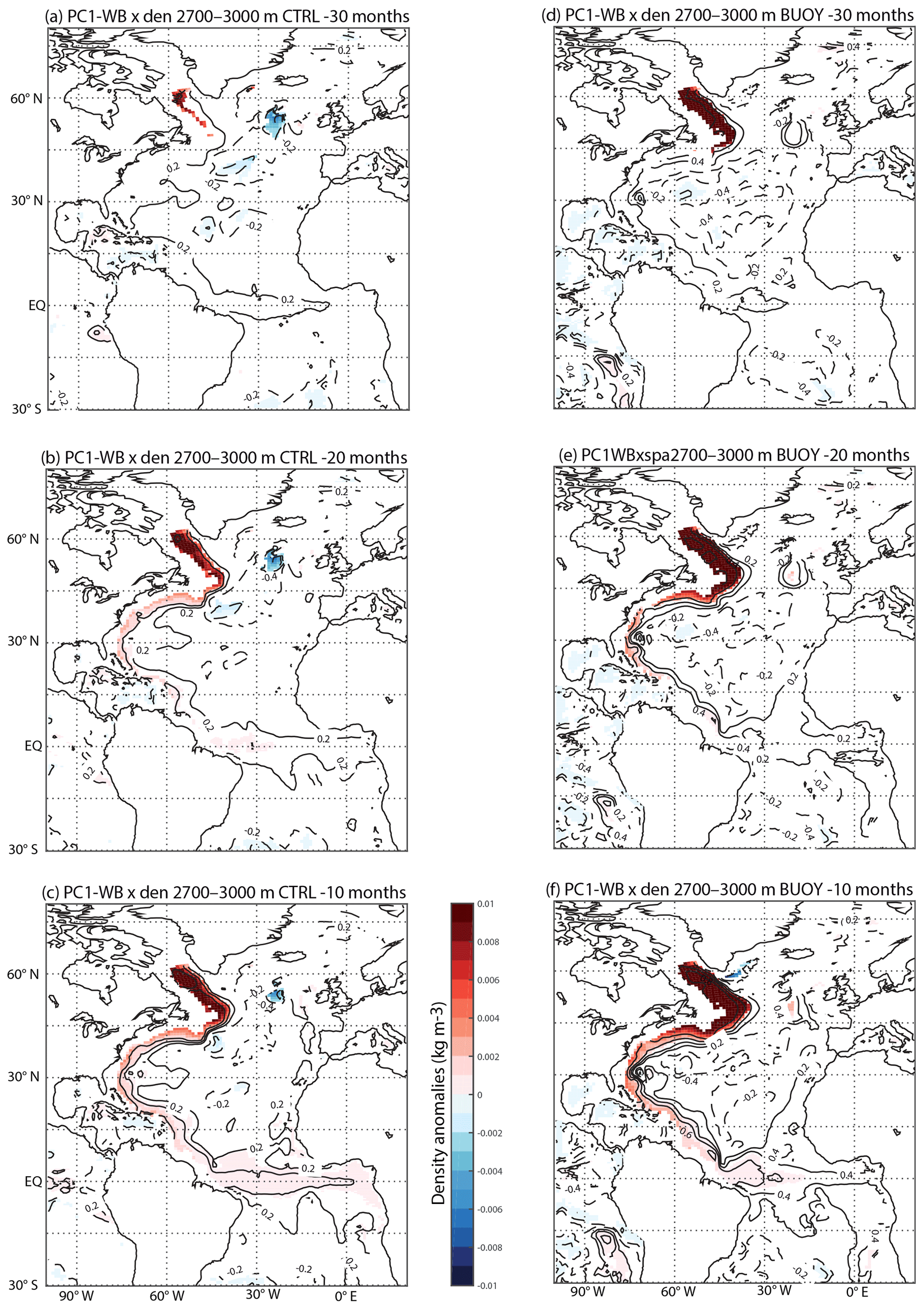
Figure 6 The spatial relationship of density anomalies with PC1-WB in the CTRL and BUOY experiments. (a) Density anomalies (in kg m⁻³) averaged from 2700 to 3000 m levels, 30 months in advance, are projected onto PC1-WB for the CTRL experiment. Black lines correspond to correlation contours every 0.2. Only significant areas are plotted with a Student's t test at 95 % confidence level, considering only effective degrees of freedom. (b, c) Same as (a) but for lags of −20 and −10 months. (d–f) Same as (a)–(c) but for the BUOY experiment.

Density regressions at shallower levels (900–1300 m) against PC1-WB in the CTRL experiment (suggested by the maximum in the EOF profiles in Fig. 4) also find anomalies beginning near the Labrador Sea, leading PC1-WB by 30 months, and a pattern of equatorial Kelvin and Rossby-waves as in Johnson and Marshall (2002) from a lag of −30 to ∼0 (Fig. S5). However, the absence of such tropical signals in BUOY at long lags (lag −30) shows that the CTRL signals could be due to wind-driven Ekman pumping (see the Supplement, Fig. S6). Therefore, we concentrate on the deeper signal which is clearly related to buoyancy.

4.2 Wave path and phase speed

Figure 7a shows the wave track defined by following the signals in Fig. 6 and using the topography at the 3269 m model level. The wave track starts in the Labrador Sea (60^∘ N) and proceeds southwards to the Equator. We plot it along the Equator and then north along the eastern boundary to 55^∘ N. The path avoids entering into the Gulf of Mexico. But at these depths this is not expected.

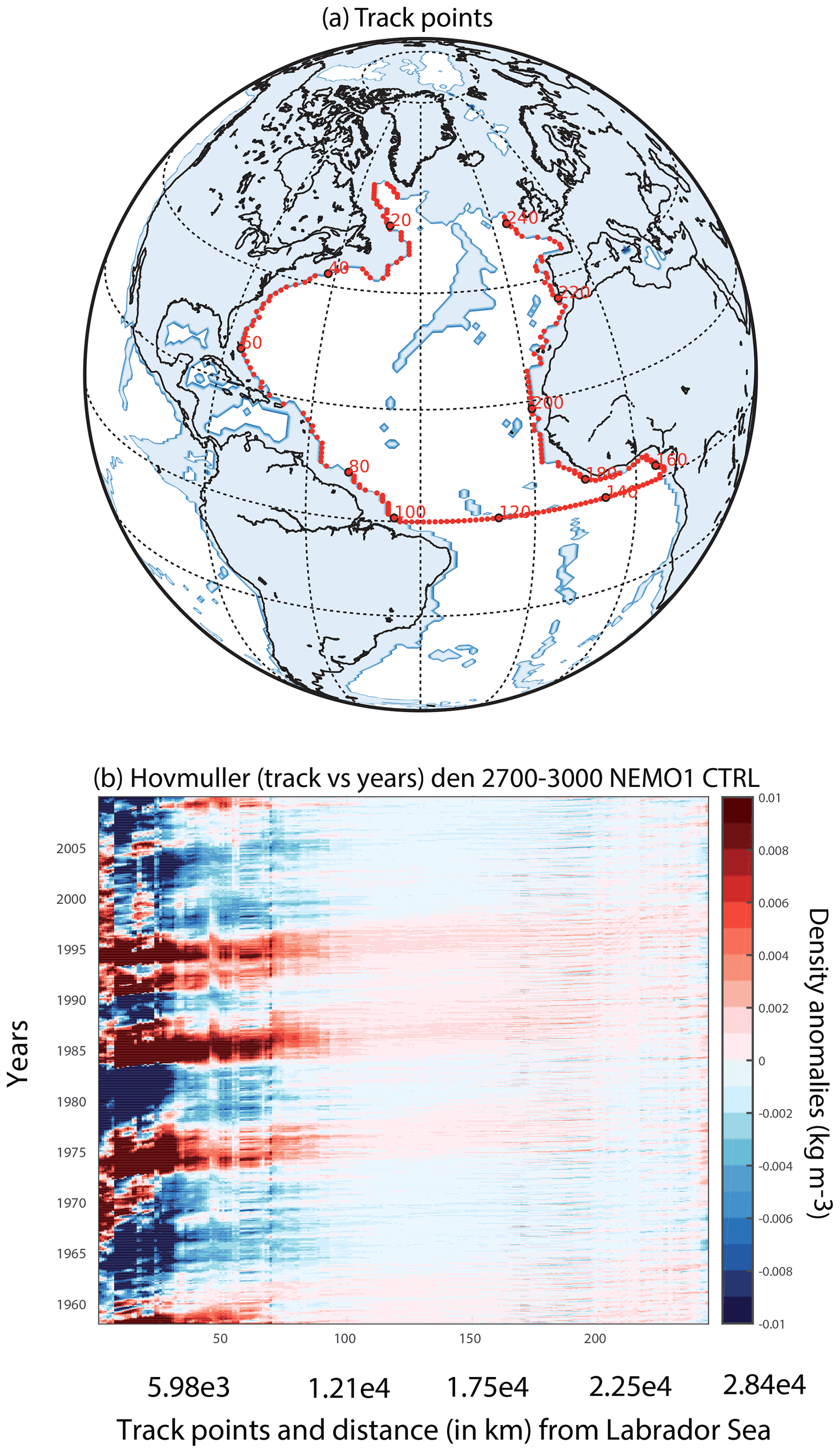
Figure 7 Hovmöller diagrams of density anomalies along the wave track in the CTRL experiment. (a) Map of the wave track used in the study. The track points correspond to the first point before the coast following the bathymetry at 3269 m. (b) Density anomalies (in kg m⁻³) along the track averaged from 2700 to 3000 m levels for the CTRL experiment. Distance (in km) from Labrador Sea is detailed together with track points on the x axis.

The Hovmöller diagram along this path (Fig. 7b) shows the propagation related to peaks in the deep water formation at high latitudes for the CTRL experiment (BUOY is very similar, not shown). Density anomalies propagate continuously along the track from the Labrador Sea around to the British Isles. The propagation shows density maxima in 1975, 1985 and 1995, also seen as peak AMOC years in Figs. 1–2. Additionally, the propagation speed from the Radon transform is similar for both experiments (0.41 and 0.31 m s⁻¹ for the BUOY and CTRL, respectively). This phase speed is consistent with the lags found between boundaries (i.e. density anomalies in CTRL will take ∼25 months to travel between WB and EB following the defined track). Background currents at the 2700–3000 m level in the CTRL are shown in the Supplement (Fig. S4).

Figure 8 shows the regression of density anomalies from Fig. 7b onto PC1-WB for the CTRL and BUOY experiments. The density anomalies in both experiments show a continuously propagating pattern from the Labrador Sea right around to 40^∘ N on the eastern boundary. The signal is stronger in BUOY, as noted in Fig. 6, but otherwise the regression patterns are very similar.

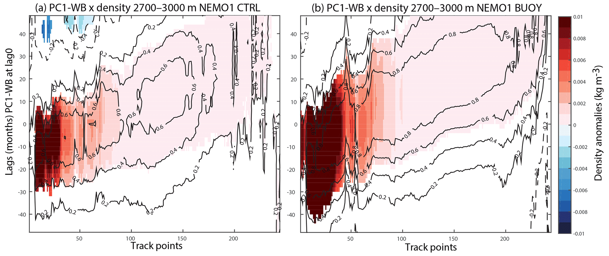
Figure 8 PC1-WB and density along the wave track. (a) Density anomalies (in kg m⁻³) averaged from 2700 to 3000 m projected onto PC1-WB for the CTRL experiment. Black lines correspond to the correlation every 0.2. Only significant areas are plotted with a Student's t test at 95 % confidence level, considering only effective degrees of freedom. (b) Same as (a) but for the BUOY experiment.

Importantly, these propagating buoyancy-related signals are clearly seen in the CTRL experiment where wind and buoyancy forcing are both applied, again suggesting that the analysis is extracting the same buoyancy-forced processes. Therefore, the diagnostic methods developed should allow for identification of similar signals in other models and in the observations. In the next section we look for similar buoyancy-forced signals in the RAPID observations.

5 Modes of WB density variability in RAPID data

The RAPID time series dataset is considerably shorter than the datasets analysed for buoyancy signals in the NEMO model. Nevertheless, Fig. 9 uses the same EOF analysis on the WB density profile for the RAPID array and for the NEMO experiments for the common period 2004–2009. The first two leading EOFs and their PCs indicate inter-annual variability in RAPID data (black lines in Fig. 9a, c). EOF1 has a maximum density anomaly at ∼1000 m (with a maximum of 0.04 kg m⁻³ in Fig. 9b), while the second mode describes variations at deeper levels (∼3000 m in Fig. 9d).

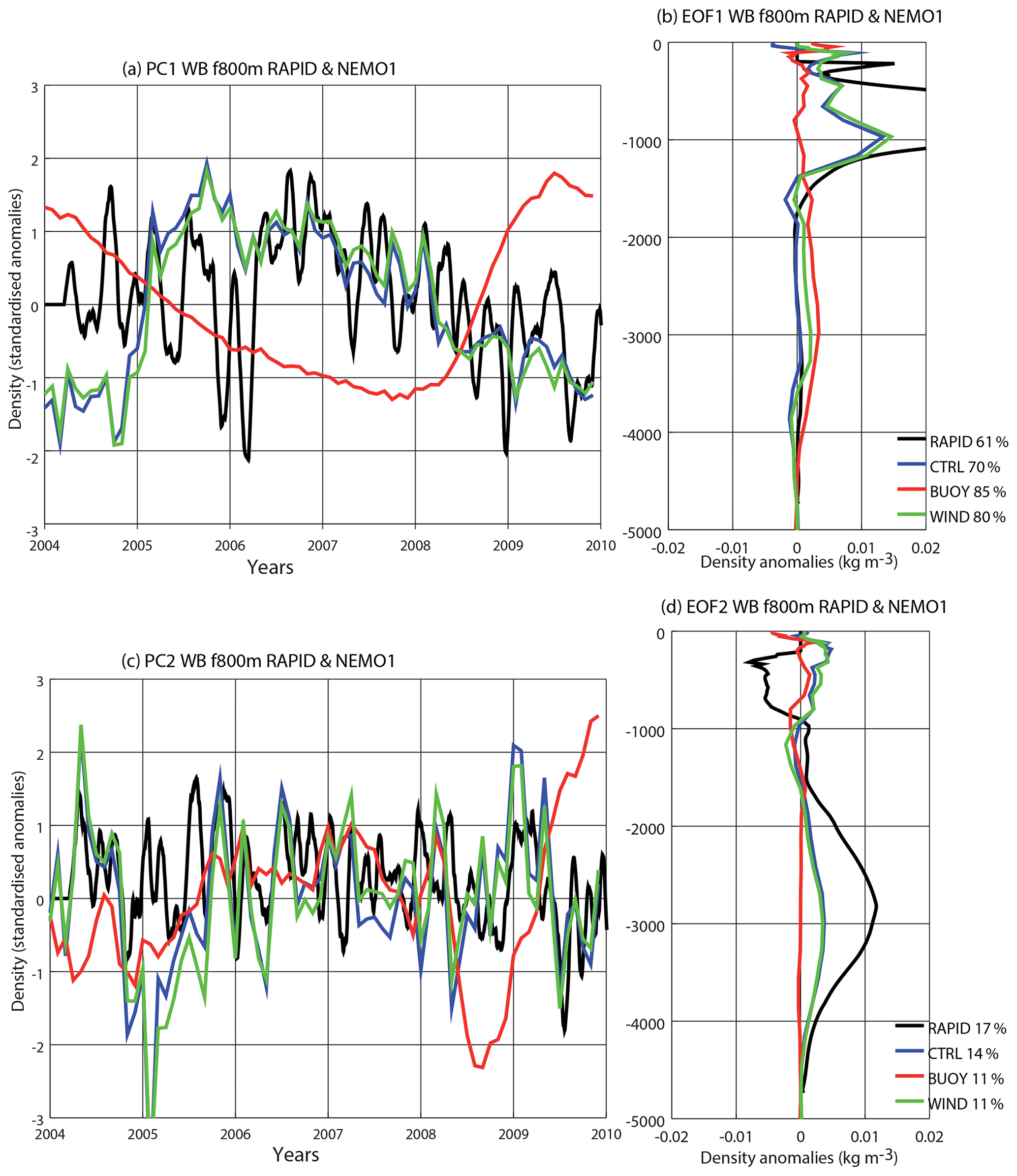
Figure 9 Leading EOFs for the NEMO experiments and the RAPID data. (a) PC time series associated with the leading EOF for the WB at 26^∘ N for the CTRL (blue line), BUOY (red line) and WIND (green line) experiments and for RAPID (black line) in the common period 2004–2009. (b) Density profiles of the EOF patterns linked to the PCs in (a). (c–d) Same as (a)–(b) but for the second mode. For this time period, the EOFs for the CTRL experiment capture wind-forced-only modes.

The density EOFs of the WB in both the CTRL (blue lines) and WIND (green lines) experiments for the common period 2004–2009 look quite similar to the EOFs from the RAPID array, in particular with EOF1 peaking at around 1000 m and EOF2 peaking much deeper at ∼3000 m (Fig. 9b, d). However, the density anomalies in the RAPID modes are larger than in the model modes (larger amplitude of density variance in RAPID compared with CTRL is also seen at all depths in Fig. S1 in the Supplement).

However, in BUOY (Fig. 9, red lines), although the deep 3000 m peak shows up as EOF1, it has very small amplitude (0.001 kg m⁻³), showing very little variability over the short 2004–2009 period. EOF1 is associated with a decrease up to 2008 and an increase thereafter up to 2010 (Fig. 9a, similar to the signal at the end of the period in Fig. 3c). BUOY EOF2 shows very little density signal at depth and mainly represents inter-annual variability (Fig. 9c–d).

The PC1 time series in CTRL and WIND also look similar to PC1 from RAPID, reaching a peak in 2007 and declining to 2010 (Fig. 9a). Therefore, for these common 6 years of simulation (2004–2009), the wind-forced inter-annual density variability on the WB is remarkably well captured by the model.

Figure 10 shows the statistics of the correlation between the leading WB mode for CTRL and both WIND (Fig. 10a) and BUOY (Fig. 10b) experiments using different numbers of years for each sub-period (x axis). Figure 10a (first box) shows the test of sampling 6-year periods (as we have in 6 years in the common period in Fig. 9a). For all 6-year sub-periods selected between 1958 and 2009, we found that EOF1 and PC1 in CTRL and WIND agreed well (Fig. 10a, first box), even in periods when the buoyancy signal was known to be changing rapidly. This dominance of the wind forcing over short time periods is not surprising and was noted previously (PA14).

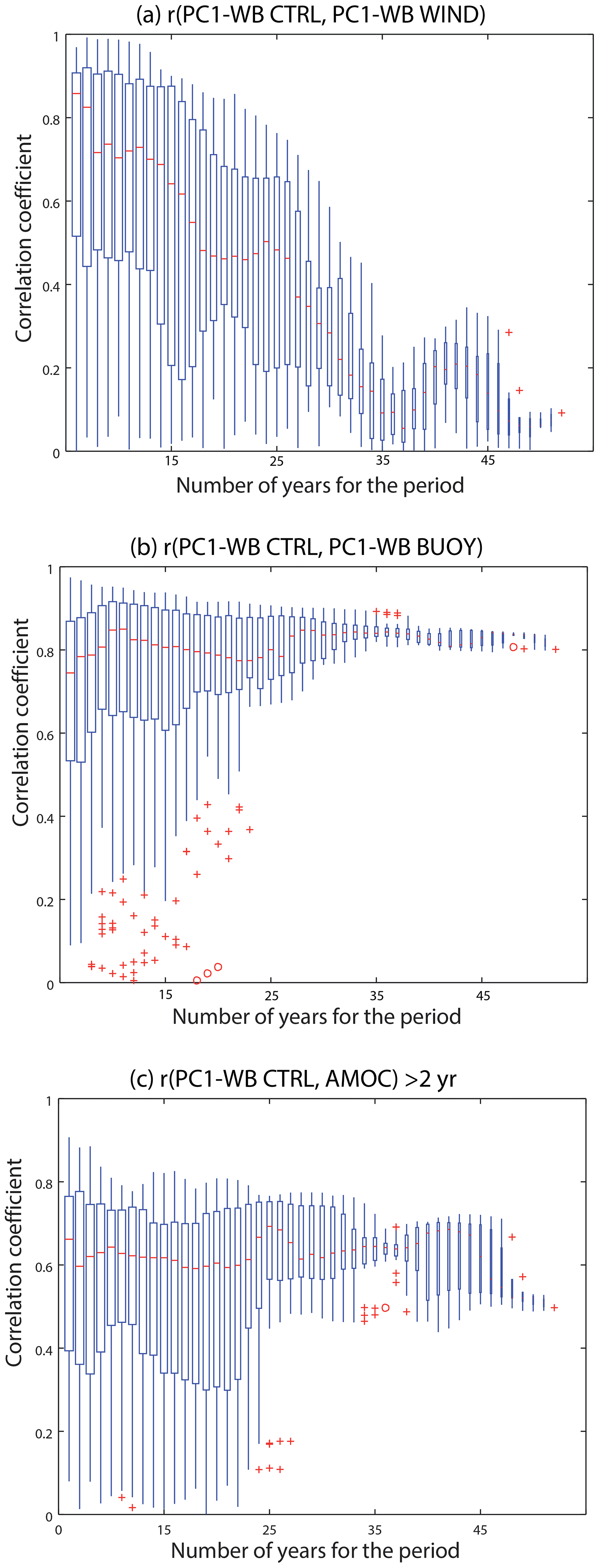
Figure 10 Impact of the number of years used in capturing the buoyancy-forced signal in CTRL. (a) Box plot of the correlation score (y axis) between PC1-WB CTRL and the PC1-WB WIND for different numbers of years (x axis) in the sub-periods considered. (b) Same as (a) but for the correlation between PC1-WB CTRL and PC1-WB BUOY. (c) Same as (a) but for the correlation between PC1-WB CTRL and AMOC filtered with periods >2 years. Red line corresponds to the median, box corresponds to the inter-quartile range (IQR), and the whiskers extend to the most extreme data points which are no more than 1.5 times the IQR from the box. Data points outside 1.5 and 3 times the IQR from the box are marked with crosses and circles, respectively. The signal extracted by PC1-WB CTRL is always a mix of forcings; however, there is a higher probability of extracting the buoyancy-forced signals when periods are longer than ∼26 years. If periods are longer than 35 years, the wind-forced signal is negligible. We have to note that for sub-periods with more years we have a smaller number of independent sub-periods and therefore there is less dispersion in the sample distribution (i.e. the box is smaller).

We find that typically 16 years of data are needed to find a significant (above 0.35) correlation between CTRL and BUOY (Fig. 10b); however, the leading mode in CTRL may still be a mix of wind and buoyancy signals (as seen from Fig. 10a). The best extraction of buoyancy forcing signals occurs when we have periods longer than 35 years, i.e. when the wind-forced signal nearly disappears (Fig. 10a). Figure 10c shows the correlation between PC1-WB and the AMOC time series for CTRL over different periods. This shows how much AMOC variance can be explained by PC1-WB. Only for periods of >25 years is PC1-WB in the CTRL experiment able to explain more than 25 % of the AMOC variance (r>0.5) and is therefore able to extract an AMOC-related signal at 26^∘ N (Fig. 10c). We note that as the sub-periods get longer, with more years (x axis), we have fewer independent sub-periods and therefore less dispersion in the sample distribution (i.e. the box is smaller). However, Fig. 10 still suggests that for long periods the correlation between PC1-WB CTRL and PC1-WB BUOY is high, the correlation between PC1-WB CTRL and PC1-WB WIND is low, and thus the WB density profile associated with PC1-CTRL is mainly a buoyancy-forced signal.

Although EOF2 data from CTRL and RAPID represent deeper density variability (Fig. 9d), they are still dominated by wind forcing over this short time period, and we note that EOF2 from WIND shows the same deep density peak. The PC2 data from CTRL and WIND show very similar time series, and even the RAPID PC2 shows a considerable level of agreement with CTRL and WIND (Fig. 9c). However, PC1 from BUOY, which has a similar EOF but represents only the buoyancy-forced component, has only lower-frequency changes with no relationship to the other time series (Fig. 9a). The BUOY PC2 time series (Fig. 9c) also shows no comparable variability.

Therefore, the short record of the RAPID array would not allow us to follow buoyancy-forced signals from the NEMO1 model. Hence, it appears likely that the variability seen here in the RAPID record, both at shallow and deeper depths, is mainly related to wind forcing (both PC1 and PC2 in the CTRL experiment and RAPID show agreement in Fig. 9). Note that the same EOF analysis using the longer record now available for RAPID data (2004–2018), but not for these model results, still gives similar density profiles to Fig. 9 (not shown).

The NEMO1 model results suggest that the lower-frequency buoyancy-forced signals from higher latitudes may start to dominate over the wind-forced signals after ∼25 years of RAPID data have been collected, when their leading density variability should show up at deeper depths (∼3000 m). In the next section we look at the ability of the analysis to extract buoyancy-forced signals, and their propagation, in a higher-resolution HadGEM3-GC2 coupled model run, which is the current UK operational coupled model.

6 Boundary density in a high-resolution coupled model

6.1 Density propagation in GC2

Figure 11a shows a wave track for the GC2 model (Sect. 2.2) bathymetry using the 3138 m level boundary, and Fig. 11b shows the Hovmöller diagram of the density anomalies for 120 years along this track after applying a 2-year low-pass filter as GC2 is much noisier at higher frequencies (see Methodology section). The high-frequency density anomalies (<2-year period) in a similar high-pass Hovmöller diagram (not shown) are very noisy and do not propagate; therefore, we suggest that the high-frequency signal is dominated by local Ekman pumping.

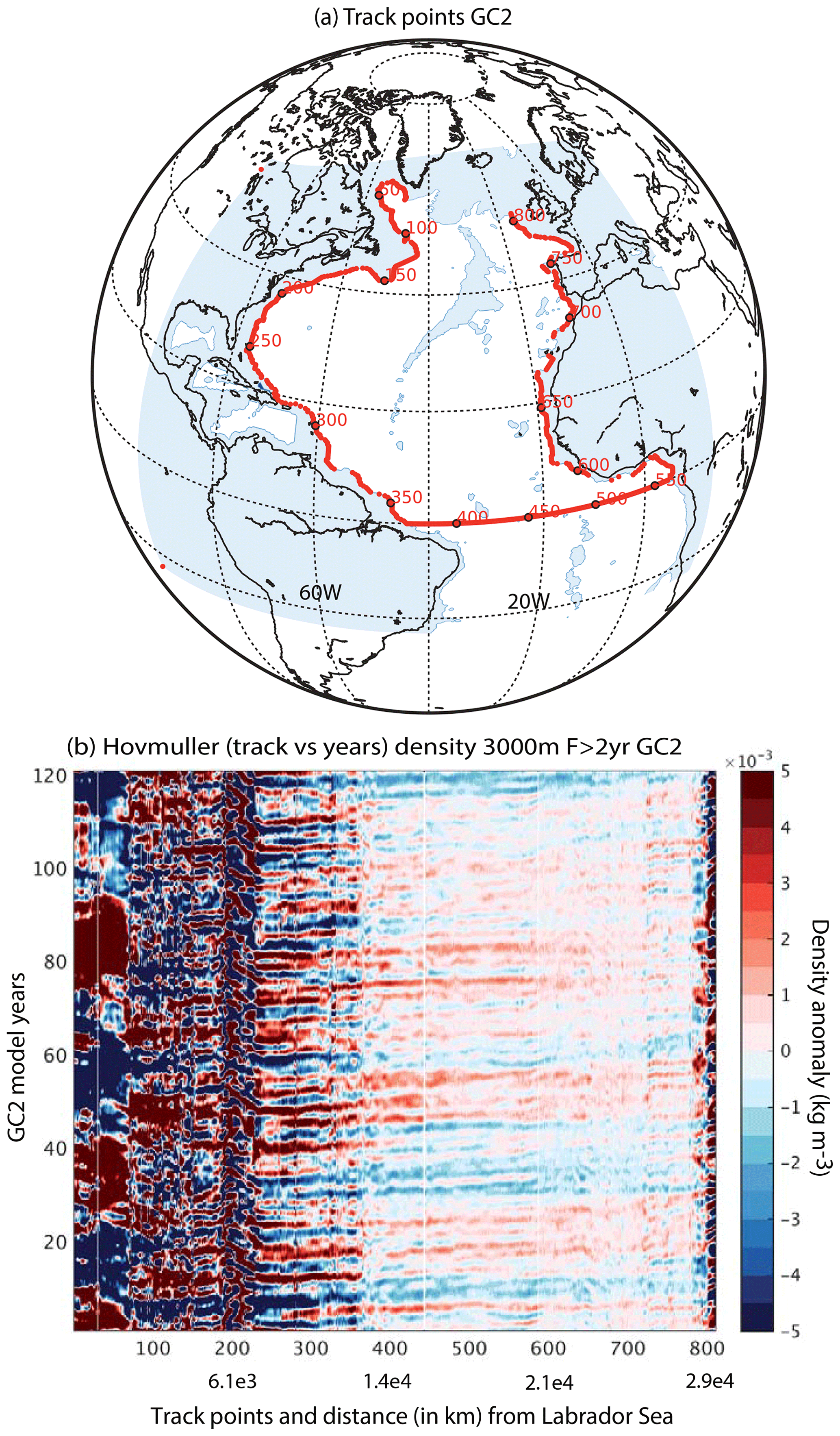
Figure 11 Hovmöller diagram of density along the wave track in the GC2 experiment. (a) The track points correspond to the first point before the coast following the bathymetry at 3138 m in GC2. (b) Hovmöller diagram of density anomalies at 3000 m along the wave track, after filtering the density time series retaining >2 years. The x axis corresponds to track points in (a), and the y axis corresponds to model year.

Anomalies propagate down the WB from ∼40^∘ N (track point 200) to the Equator and across to the EB. These signals can be traced back across the Gulf Stream to subpolar latitudes (points 100–200), but only appear as lower-frequency decadal variations in the subpolar gyre and into the Labrador Sea (points 0–100). The Radon transform phase speed is ∼2 m s⁻¹, which is faster than the phase speed calculated in NEMO1 at the same depth (Fig. 7), and closer to the theoretical and observed Kelvin wave propagation speeds (Illig et al., 2004; Polo et al., 2008). Other authors, using models of different complexity, have found a similar phase speed of density anomalies from AMOC variations propagating along the western boundary (Getzlaff et al., 2005; Zhang, 2010; Marshall and Johnson, 2013). Therefore, as the density anomalies propagate down the deep western boundary, we would expect to find this deep density variability signal using the EOF analysis.

6.2 EOFs at the WB in GC2

Figure 12a shows the vertical density profiles associated with the first two EOFs from 800 m downwards at the 26^∘ N WB in the GC2 experiment. The profile location is the closest grid point to the western wall at the Bahamas, which reaches the bottom at 3200 m, and the first two EOFs explain more than 70 % of the total density variance. EOF1 shows an equivalent barotropic vertical structure peaking near the bottom (∼3000 m, blue line), while EOF2 changes sign between 900 and 3000 m (red line).

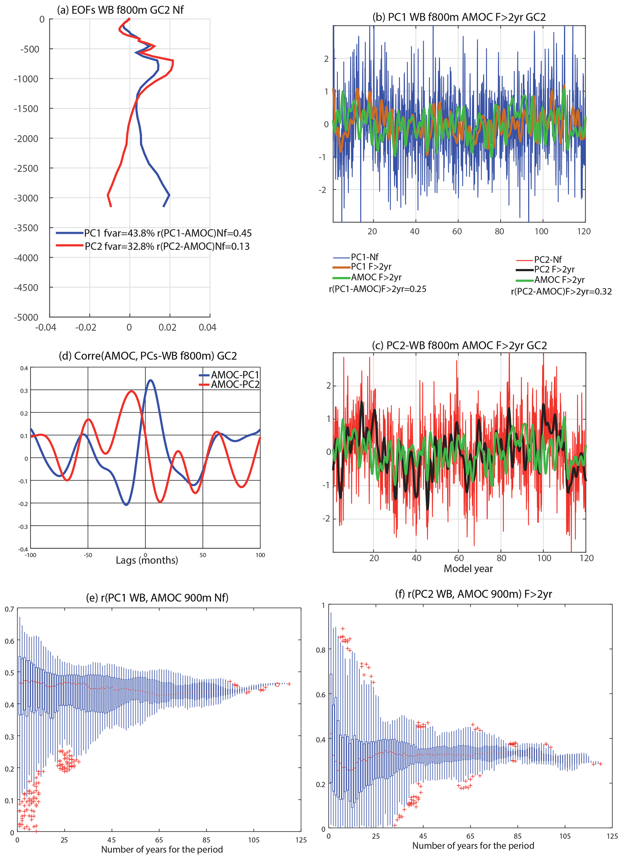
Figure 12 EOFs of WB density profiles at 26^∘ N in the GC2 experiment. (a) Leading (blue line) and second (red line) EOFs from the WB at 26^∘ N, 76.75^∘ W in the GC2 experiment are shown. Percentage of explained variance and correlation with the AMOC time series defined at 26^∘ N and 925 m depth are displayed. (b) Time series associated with leading EOF-WB (PC1-WB, blue line), PC1-WB filtered time series (PC1-F > 2 year, brown line) and the AMOC filtered time series (AMOC-F > 2 year, green line) are shown. (c) Same as (b) but for the PC2-WB. (d) Correlation between AMOC (at lag 0) and the first two PC-WB series (lagged). (e) Correlation between PC1-WB and AMOC time series. Box plot is similar to Fig. 10c. The x axis represents the number of years used in the periods for the correlation; the y axis represents correlation score. (f) Same as (e) but for the correlation between PC2-WB and AMOC filtered with periodicity >2 years.

Table 2 Correlations between PCs f_800 m WB and AMOC time series in GC2. Correlations between the geostrophic AMOC and the PCs at the WB for the GC2 experiment. Significant correlations are highlighted with a star (^∗) based on a t test at 95 % confidence level and after calculating the number of effective degrees of freedom.

The PC1 time series associated with EOF1 is plotted in Fig. 12b (blue line). Unlike in NEMO1, this PC1 shows high-frequency variability which is nevertheless still correlated with the AMOC minus Ekman component (i.e. the peak AMOC stream function at 900 m after the variability due to Ekman has been removed) without filtering at r=0.45, rising to r=0.49 with high-pass (<2 years) filtering. However, PC1 becomes less correlated with the AMOC after 2-year low-pass filtering, r=0.25 (Table 2). In contrast, for PC2 the unfiltered correlation with the AMOC minus Ekman component is low (r=0.13), but this increases with a 2-year low-pass filtering (r=0.32, Fig. 12c, Table 2). As density anomalies at deep levels are able to be excited by wind alone (already seen in both NEMO1 and the RAPID observations in Fig. 9), the two EOFs in GC2 each capture some wind and some buoyancy forcing.

Although PC1 and PC2 are orthogonal by construction, and thus correlation between time series is zero, after time filtering the PCs the modes are correlated (r=0.41) and the lead–lag correlations with the AMOC present a cycle between vertical profile modes, with 16 months between the peaks (Fig. 12d). This indicates the limitations of extracting low-frequency AMOC-related signals in more complex environments using linear methods.

The high-frequency PC1-WB (<2 years) represents a high-frequency density signal at 26^∘ N, which could be wind-forced. It is correlated with the AMOC and is independent of the number of years used to identify it (Fig. 12e). PC2-WB correlates better with a lower-frequency AMOC signal (>2 years) and is also independent of the number of years used to identify it (Fig. 12f).

If we filter the density anomalies prior to performing the EOF, then the leading mode corresponds to PC2-WB seen here. This confirms that we cannot isolate the low frequencies by identifying a deep density signature, as works well in NEMO1; therefore, time filtering is needed to identify the inter-annual buoyancy signal in GC2 as a leading mode. Nevertheless, the buoyancy signal is still traceable emerging from the Labrador Sea and is well captured in the PCs, representing relevant information on AMOC variability.

Here we summarise the comparison between density profile modes in different environments as follows.

• i.

  In the NEMO1 CTRL simulation with 52 years of data, we can find a vertical density pattern at 26^∘ N that is buoyancy forced (i.e. similar to the mode in the BUOY experiment). This has maximum density anomalies at 1500–3000 m and corresponds to low-frequency variability of the AMOC. The source is the density changes over the Labrador Sea. In comparison, the leading density mode for the WIND experiment has a maximum at 1000 m and represents inter-annual variability of the AMOC.

• ii.

  However, if the same methodology is applied over shorter periods, the wind-forced variability dominates the first two EOFs, with density anomalies at 1000 and 3000 m. The limit for the time period is about 25 years to extract buoyancy-forced signals that can be related to the AMOC at lower frequencies.

• iii.

  When CTRL is compared with the RAPID array PCs, we find similar vertical profiles in the CTRL and observed PCs, suggesting that the short period of RAPID does not allow us to extract relevant buoyancy signals. Wind-forced signals are predominant, showing density anomalies that are also relevant for the geostrophic part of the AMOC at 1000 m (but without any lag and at inter-annual timescales).

• iv.

  The same methodology applied to a more complex GC2 Earth system model results in a leading PC that shows positive anomalies between 1000 and 3000 m. This PC1 is related to the AMOC at short inter-annual timescales (predominantly wind forced). The PC2 mode shows reversing density anomalies between 1000 and 3000 m and is related to the AMOC at lower frequencies (period >2 years). The analysis shows that these PC1 modes are correlated to AMOC independently of the number of years used in the calculation, although correlation with PC1 has less spread for sub-periods longer than ∼26 years (Fig. 12e–f).

The EOF below 800 m method seems to be appropriate to detect buoyancy-forced signals from density profiles if we have more than ∼25 years of data in NEMO1. However, a Lanczos time filtering for periods >2 years prior to the EOF analysis is recommended in more complex environments, as would be required for RAPID observations, and for coupled models. From similarities between NEMO, RAPID and GC2, we conclude that the density profile mode that is likely to be buoyancy forced, corresponds to density anomalies at deep levels (3000 m) that covary negatively with density anomalies at upper levels (1000 m). Time series should be filtered with periods >2 years and the PC should then correlate with the AMOC at 26^∘ N (1000 m) for the same frequencies.

7 Discussion

In this work we have used model output and statistical methods to identify vertical density profiles along the boundaries that are consistent with the buoyancy-forced variability. We have shown that the most relevant profile at 26^∘ N is found at the WB using EOF analysis after truncating the density profile from 800 m (PC1-WB). This truncation is very effective in emphasising low-frequency (decadal timescale) signals, and in NEMO1 it negates the need for temporal filtering, which can also add spurious signals or lead to excess smoothing. Caveats that warrant further discussion include the differences between the EOFs in NEMO1 and GC2 and the role of the EB.

We note that vertical profiles of the WB EOFs in GC2 and NEMO1 are different, especially in the top 1500 m, and the frequencies of the dominant variability in boundary signals in GC2 are higher than the decadal signature seen in NEMO1. We find that shallow (<1500 m) density signals related to PC1-WB in NEMO1 have different timing in CTRL and BUOY experiments in the tropics (Figs. S5–S6), suggesting that at 26^∘ N wind forcing is modulating the buoyancy-forced density signal in CTRL. This is also an argument to suggest that in GC2 the shallow signal is probably a wind-forced signal.

Although PCs in GC2 contain the low-frequency AMOC-related variance, it is perhaps not surprising that the details of the WB EOFs are different to those in NEMO1, given the range of AMOC variability in models (Biastoch et al., 2008; Cabanes et al., 2008; PA14; Ortega et al., 2017). The 1^∘ horizontal resolution, and even the 1∕4^∘ model, may still be too coarse to correctly capture propagating boundary signals (Johnson and Marshall, 2002; Getzlaff et al., 2005; Hodson and Sutton, 2012) from the Labrador Sea. Therefore, we may not expect the exact details of the boundary density EOFs (or the phase speeds or phase lags identified from the boundary and Labrador Sea signals) to be very realistic. Nevertheless, the methods reveal, in two very different modelling environments, boundary signals consistently related to the geostrophic AMOC at 26^∘ N.

Regarding the differences in the phase speed propagation in NEMO1 and GC2, there are factors that influence propagation (and hence the phase speed) of boundary waves in numerical models such as (i) model resolution (Hsieh et al., 1983; Hodson and Sutton, 2012), (ii) lateral viscosity (Davey et al., 1983), (iii) orientation of the coastal boundary relative to the ocean grid (Schwab and Beletsky, 1998), (iv) ocean stratification along the propagation trajectory and (v) additional complexity in a coupled model in comparison with an ocean-only model, potentially influencing the propagation. We think that both resolution and complexity are explaining the differences in the phase speed along boundaries shown in the Hovmöller plots (Figs. 7 and 11); however, specific sensitivity experiments should be designed in order to properly understand these factors.

It is also worth noticing that, due to noise from high-frequency wind forcing, time filtering is needed to see a more clear buoyancy-related signal in GC2. Wind forcing can be projected onto density anomalies at deep levels (as is seen in the RAPID data and in GC2), and similar time filtering may be needed in the observations in order to extract the buoyancy-forced signals. Understanding the differences between these boundary density EOFs between models would be useful for interpreting observations as the RAPID record becomes longer, and it should be a focus of further work.

In Sect. 3.3, we tested the value of using WB and EB together in a single EOF. The fact that combining the WB and EB at different lags does not improve the explained variance shows that the WB alone captures most of the variability at decadal timescales. This is in agreement with previous results by PA14 and also with the propagating signal from the Labrador Sea that can reach the subtropics along the WB (as shown by Jackson et al., 2016), but the propagation up the EB is less clear. This is not to say that the EB observations do not make up an important component of the RAPID array observations. Indeed, it has already been shown, in observations (Kanzow et al., 2010; Duchez et al., 2014) and in models (PA14), that the EB is important for understanding the wind-forced variability in the observed AMOC at 26^∘ N from sub-annual to inter-annual timescales. Here we were able to show the density propagation at 3000 m depth on the EB, which has a clear AMOC-related signature, although with a lag. Therefore, the EB observations are still important in understanding the role of decadal buoyancy-forced variability.

We want to comment that the correspondence of the PCs and boundary wave modes is not direct. The boundary EOFs only capture variability at single locations (26^∘ N). Figure 4 shows that the teleconnection between density signals at the WB and EB occurs very quickly at 800–1100 m (around 8 months as a fast response). However, at deeper levels the EB signal is delayed. The different lags in Fig. 5 reflect different propagation speeds at different depths, mainly along the Equator. (Hovmöller diagrams at different depths suggest that the phase speeds change at the Equator.) The propagation along either the WB or the EB represents boundary waves with more coherent EOF vertical modes, albeit different modes on the WB and EB.

The temporal variability in the RAPID WB density profile suggests that wind forcing is still the dominating variability in the short record. More years of RAPID data may be needed to allow the buoyancy-forced variance to appear in the leading EOFs. Although it may be helpful to perform time filtering which could allow the buoyancy-forced signal to be found in shorter periods of data, the continuation of the RAPID array would be crucial in order to understand the wind-forced inter-annual variability and to detect the density signals linking the subpolar North Atlantic with the AMOC at 26^∘ N.

8 Conclusions

In this work we have used NEMO1 OGCM experiments which separate buoyancy and wind-forced signals (BUOY and WIND experiments; Polo et al., 2014), together with statistical techniques, to develop methods to extract the Atlantic boundary density profile signatures at 26^∘ N most associated with the buoyancy-forced AMOC from an experiment with both buoyancy and wind-forced variability (CTRL). After finding the “best” vertical profile on the western boundary, we describe the spatio-temporal structures related to this signal. The main findings are summarised as follows:

• Using EOF analysis and outputs from OGCM experiments, we find that the vertical density structure at both the western (WB) and eastern boundaries (EB) at 26^∘ N show characteristics that can be unambiguously linked to buoyancy forcing in the Labrador Sea.

• The vertical structure associated with the leading EOF mode of density variability on the WB (EOF1-WB) shows positive anomalies from 1500 to 3000 m depth that can be related to earlier changes in the North Atlantic Deep Water formation and to density anomalies over the Labrador Sea, which are seen to lead PC1-WB by ∼30 months. PC1-WB is found to be very robust in both the CTRL and BUOY experiments, driving buoyancy-forced AMOC variability on decadal timescales. PC1-WB explains 40 % and 70 % of the 26^∘ N deep density variance for the CTRL and BUOY experiments, respectively.

• PC1-WB is found to lead density anomalies at 1000–1500 m on the EB (associated with PC1-EB) by ∼ 7 months. The result of combining both boundaries into a single density EOF allows us to extract the correlated variance and the optimal lag between the boundaries. The combined EOF variance shows maxima when lagging the EB between 7 months and 3 years. The longer-period lagged relationship is consistent with density propagation at 2700–3000 m.

• In the CTRL experiment, density anomalies at 2000–3000 m propagate southwards along the WB, eastward along the Equator and then up to the African coast, impacting the vertical structure on both boundaries at 26^∘ N. The propagation is continuous from the Labrador Sea around the basin and up to the British Isles. This density signal propagates at an average speed of ∼ 0.3 m s⁻¹, consistent with the propagation speeds in the BUOY experiment.

• The same method is applied to the RAPID array data for the common period with the NEMO1 simulations. The two leading EOFs for the WB have anomalous densities at 1000 and 3000 m and are well simulated by the CTRL experiment (Fig. 9). This inter-annual variability is unequivocally wind forced. The observational record must be longer in order to identify the buoyancy-forced vertical anomalies, which have lower frequencies.

• The same method was able to extract boundary signals from the higher-resolution model HadGEM3-GC2. Despite the greater complexity in GC2, the vertical density profiles on the WB at 26^∘ N can be clearly related to the geostrophic AMOC, although some time filtering is needed in order to separate the timescales.

• After filtering (periods below and above 2 years), PC1-WB is found to be more related to AMOC at 1000 m at high frequencies, with an EOF profile with strong positive density anomalies at 1000 and 3000 m. PC2-WB is related to the AMOC at 1000 m at low frequencies and shows positive (negative) density anomalies at deep 1000 m (3000 m) levels.

• We also show clear density propagation from the Labrador Sea around the basin to the British Isles along a wave track at 3000 m depth (defined by 3138 m bathymetry), which explains part of the AMOC variability. However, temporal filtering is needed to make this stand out above the noise.

• We conclude that the buoyancy-forced density signals at 26^∘ N will be distinguishable in the observations (as well as in coupled models) if the available record is long enough (>26 years), selecting density profiles with opposite anomalies at 1000 and 3000–3500 m, with time filtering >2 years to help eliminate high-frequency wind-driven signals.