AMOC weakening across latitude and time in CMIP6 future scenarios

The Atlantic Meridional Overturning Circulation (AMOC) is projected to weaken in the latest generation of climate models used in the Coupled Model Intercomparison Project, Phase 6 (CMIP6). This study investigates the latitudinal coherence of this AMOC weakening and how it differs across depth- and density-space, future forcing scenarios and individual models. Percentage AMOC weakening is presented as a function of latitude and time between 1900 and 2100. By identifying the first year when specific percentage thresholds of weakening are reached at each latitude, contour lines of weakening are mapped as a function of latitude and time. Propagation of AMOC weakening is inferred from the gradient of these lines (defined as weakening gradients). Percentage weakening is found to originate at high latitudes (45–51° N in depth-space and 51–61° N in density-space) and propagate southwards. Because density-space weakening originates further north than depth-space, it has a longer lead time for propagation and our results suggest it could provide a more effective framework for early warning signal development. South of 40° N, propagation speeds in depth-space and density-space representations are similar. In the most extreme future forcing scenario, the multi-model mean weakening gradient reduces from ∼ 3.0 to ∼ 1.4° yr⁻¹, implying that as the AMOC weakens so too does the propagation of AMOC weakening. This behaviour is also seen for the majority of models (67 %). For a small fraction of models (13 %) the weakening gradients increase as the AMOC weakens and for the remainder (20 %) there is no discernable trend. The weakening gradients reduce more steeply in less extreme future forcing scenarios than in more extreme ones. The initial speed of propagation is found to be positively related to historical AMOC strength.

1 Introduction

The Atlantic Meridional Overturning Circulation (AMOC) is an important component of large-scale global ocean circulation. It is characterised by northward flow of warm and salty surface water, densification of water at high latitudes and the southward return flow of colder, fresher deep water. Europe's mild climate is due to the AMOC transporting heat northward, it is responsible for 0.5 PW of cross-equatorial heat transport (Trenberth and Fasullo, 2017) and 1.2 PW northward heat transport at 26.5° N (Johns et al., 2023).

The latest generation of climate models in the Coupled Model Intercomparison Project, phase 6 (CMIP6) (Eyring et al., 2016) predict the AMOC will weaken on average by 24 %–39 % by 2100 dependent on future scenario (Weijer et al., 2020; Fox-Kemper et al., 2021). A weakened AMOC will have significant weather and climate risk for Europe such as an increased risk of heatwaves (Meccia et al., 2025), although they may be less severe with a weakened AMOC (Duarte et al., 2025), enhanced storm tracks over Northwestern Europe (van Westen and Baatsen, 2025; Vacca et al., 2025) and lagged warming compared to the rest of the world (van Westen and Baatsen, 2025; Vacca et al., 2025). On top of the localised impacts, there are a variety of global climate impacts associated with a weakened AMOC (e.g. changes to precipitation patterns Bellomo et al., 2021; Jackson et al., 2015, reduced northern hemisphere temperatures Jackson et al., 2015; Liu et al., 2020 and a poleward shift of northern hemisphere midlatitude jets Liu et al., 2020; Bellomo et al., 2021). The large uncertainties on the magnitude of AMOC weakening are linked to model differences between the CMIP6 ensemble, e.g. due to mean state AMOC strength (Jackson et al., 2020; Lin et al., 2023), connectivity between the Atlantic and Indo-Pacific (Baker et al., 2023) and parametrisation schemes (Zhao et al., 2024). Improved understanding of the model differences could be used to improve model simulations, constrain existing AMOC projections and increase confidence in predictions of future impacts. There is also uncertainty as to whether or not the AMOC will reach a tipping point. While the latest IPCC report deemed it as 'low probability' by 2100, there is evidence that suggests the AMOC is more likely to tip this century than CMIP6 predictions (Van Westen et al., 2024). For some CMIP6 models, it has been shown the AMOC experiences a tipping point in deep convection within the before 2100 (Drijfhout et al., 2025). The possibility of AMOC tipping adds to model uncertainty and while it is not the focus of this study, it is worth considering the model biases potentially related to an overly stable AMOC (e.g. Mecking et al., 2017).

A general mechanism for AMOC weakening under climate forcing was proposed by Haskins et al. (2020) through the use of hosed experiments: freshening of the surface layer occurs due to changes in the water cycle, the fresh layer inhibits heat exchange with the atmosphere, preventing cooling, and results in a subsurface warm “blob”. The warm blob increases stratification across the surface, reducing the formation of North Atlantic Deep Water (NADW) as well as adjusting the zonal pressure gradients through the increased subsurface temperature anomaly, which weakens the AMOC. A similar mechanism was shown by Levang and Schmitt (2020) for CMIP5 high emissions scenarios, with a focus on the heat brought north from the subtropics. This general temperature-driven mechanism of weakening has been shown both as a response to climate forcing (Levang and Schmitt, 2020) as well as freshwater hosing (Haskins et al., 2020; Gérard and Crucifix, 2024). There are numerous studies on AMOC weakening in CMIP6, typically using an AMOC index at specific latitudes such as 26.5° N, the latitude of the RAPID array (Weijer et al., 2020; Bryden et al., 2024; Madan et al., 2023). However, the latitudinal structure of AMOC weakening and possible differences across CMIP6 future projections are poorly understood.

Latitudinal connectivity of the AMOC is an active area of research, particularly regarding the propagation of density anomalies and understanding multi-decadal variability. The timescale of interest plays a key role in understanding the meridional coherence of the AMOC. Fast connectivity of density anomalies between the subpolar and subtropical gyres (with the subtropical lagging the subpolar on the order of 1–2 years) has been found by studying observational arrays (Wett et al., 2023; Han, 2023). Coherence between the Labrador Sea and the subtropical gyre has also been assessed in model studies, showing a lag in density anomalies on the order of 3–4 years (Zhang, 2010; Zou et al., 2019; Kostov et al., 2022) while others show a lag of between 5-10 years, a result that is model dependent (Li et al., 2019). One potential reason for this difference is the resolution of the models. Higher resolution models that resolve eddies have been shown to propagate tracer (e.g. salinity) signals faster along the Deep Western Boundary Current (DWBC) than in non-eddying models (Weijer et al., 2012). Models that do not resolve eddies and the Rossby deformation radius struggle to accurately capture propagation speed along the boundary (Marshall and Johnson, 2013) and parameterisation in coarse resolution models could explain differences in propagation speed. The presence of eddies in models has also been shown to impact the rate and severity of AMOC decline due to freshwater hosing (Den Toom et al., 2014; van Westen et al., 2025). Most CMIP6 ocean models have (nominally) 1 degree resolution and do not resolve eddies but some modelling centres provide higher resolution versions.

Zhang (2010) propose that north of 35° N advection by mean flow is the mechanism that transports density anomalies and that south of 35° N density anomalies are transported by coastal Kelvin waves. The relationship between changes to densification in the SPG and AMOC strength south of the SPG (at 45° N) was the subject of a recent modelling study by Petit et al. (2025), where the authors found coherence was facilitated by the shoaling of isopycnals along the DWBC resulting in changes to the zonal density gradient. This response occurs on the order of months. They also noted no coherence between AMOC strength between the OSNAP arrays and 45° N. The role wind plays in the connectivity of the AMOC is complex, with Zou et al. (2019) highlighting that meridional coherence can be driven by wind forcing as well as by buoyancy forcing while Fraser et al. (2025) discuss that wind driven Ekman pumping can disrupt meridional coherence in both depth and density-space representations of the AMOC.

The AMOC responds to high latitude buoyancy forcing on many time scales, from months and years to slow adjustments to the mean state on multi-decadal timescales (Gu et al., 2020). Proposed mechanisms that facilitate this adjustment include the slow advection of anomalies through the DWBC (Gerdes and Köberle, 1995; Hodson and Sutton, 2012; Zhao et al., 2017) where adjustment can take on the order 100 years (Marotzke and Klinger, 2000), or a baroclinic adjustment of the ocean interior from Rossby waves mediated by equatorial Kelvin waves (Döscher et al., 1994; Marshall and Johnson, 2013). The decadal changes to the structure of the AMOC in response to climate change, rather than annual variability of density anomalies, is the focus of this study.

The AMOC can be represented by overturning streamfunctions in depth-space, with latitude-depth coordinates, and in density-space, with latitude-density coordinates. The depth-space AMOC best represents vertical mass flux while the density-space AMOC better captures water mass transformation, particularly at high latitudes (Hirschi et al., 2020). The depth-space AMOC is more straightforward to compute and has historically been used more commonly than the density-space AMOC. Density-space AMOC has gained popularity because of its description of water mass transformation, particularly in the sub-polar North Atlantic (Buckley et al., 2023; Straneo, 2006; Pickart and Spall, 2007). Propagation differences of weakening between a depth-space and density-space were explored by Kwon and Frankignoul (2014), considered in the context of a 20 year cycle of AMOC variability and showing at depth a broadly southward propagation of weakening for both representations.

The focus of this study is to understand the latitudinal and basin-wide changes to the AMOC under CMIP6 future scenario forcing, both in the multi-model mean and individual models, and to understand how AMOC weakening propagates through the basin. This study uses a new technique to investigate latitudinal connectivity of AMOC weakening using exclusively the streamfunction. Specifically, we consider the AMOC decline across the basin rather than at select latitude to deliver new insights into the latitudinal connectivity of AMOC weakening for the CMIP6 model set. The analysis is split into three sections. The first section is on the differences of AMOC weakening and propagation speed in depth-space and density-space representations of the AMOC, using the multi-model mean and in experiments under a high emission scenario. The second section is on the differences of the basin-wide response between future climate forcing scenarios of the multi-model mean. The third section explores individual model differences of the propagation speed of weakening and categorises models according to those differences.

2 Methods and Data

2.1 CMIP6 Models

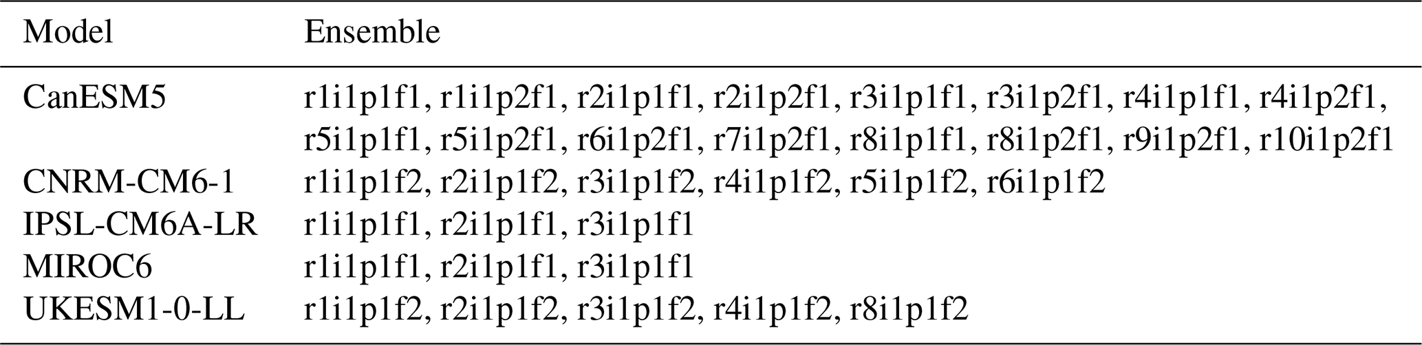
This study analyses data from 15 models from the Coupled Model Intercomparison Project Phase 6 (CMIP6) (Eyring et al., 2016). Historical experiments, using historical external forcing, simulating 1850–2014 (Eyring et al., 2016) and four ScenarioMIP future projections for 2015–2100 (O'Neill et al., 2016); ssp126 (low emission), ssp245 (medium emission), ssp370 and ssp585 (high emission) are investigated. Since the focus of this study is the AMOC streamfunction, the models selected require the necessary monthly-resolution variables to compute them for both depth- and density-space: meridional velocity (vo), practical salinity (so) and potential temperature (thetao) for the historical and all the previously mentioned ScenarioMIP experiments. Additionally, where available, variable vertical thickness (thkcello) is used in density streamfunction calculations. The exceptions to this are ACCESS-CM2 and ACCESS-ESM1-5, which lack sufficient vo on JASMIN for all scenarios but have computed depth-space streamfunctions available. We also choose to use the provided density-space streamfunctions for sigma-level models. This is to avoid issues with interpolating from sigma-levels to depth-levels and back to sigma-levels. These requirements limit the number of models in this study to 15. For consistency, priority is given to offline computed streamfunctions over the provided streamfunctions. As many ensemble members were used as possible. The variables used for each CMIP6 model in this study are listed in Table 1 and for models with multiple ensemble members, they are listed in Table 2. For models with multiple ensemble members, the ensemble mean values are used unless otherwise specified.

Bi et al. (2020)Ziehn et al. (2020)Swart et al. (2019)Zhang et al. (2020)Danabasoglu et al. (2020)Lovato et al. (2022)Voldoire et al. (2019)Döscher et al. (2022)Döscher et al. (2022)Boucher et al. (2020)Tatebe et al. (2019)Yukimoto et al. (2019)Seland et al. (2020)Sellar et al. (2019)Wang et al. (2021)

Table 1 The CMIP6 models used this study, listed with their institution, the variables and the ensemble member used. For models with multiple ensemble members, see Table 2. Streamfunctions provided by the modelling centres are labelled “msftmz” for depth-space and “msftmrho” for density-space. Calculated streamfunctions are labelled by the variables they are calculated with: “vo” (meridional velocity) for depth-space and “vo”, “so” (absolute salinity), “thetao” (conservative temperature) and when available “thkcello” (variable vertical thickness) for density-space.

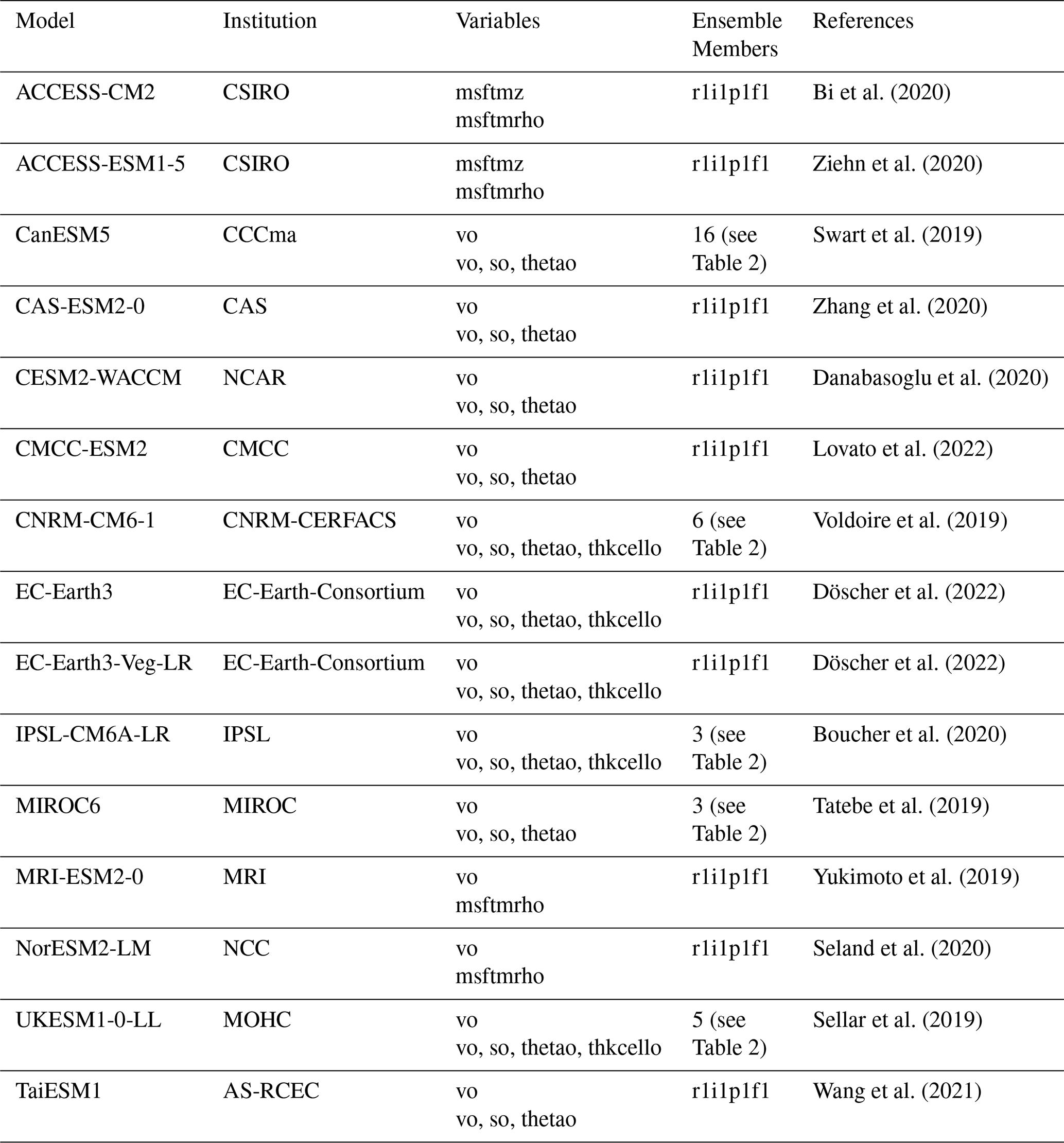
Table 2 The ensemble members used for models with multiple ensemble members.

2.2 AMOC Streamfunction

The depth-space streamfunction is computed with Eq. (1), integrating the meridional velocity (“vo”).

The depth-space streamfunctions were calculated by the integral as described in Hirschi and Marotzke (2007),

$$\begin{array}{}\text{(1)}& {\mathit{\psi }}_z(y,z^{\prime },t)=\underset{x_{\mathrm{w}}}{\overset{x_{\mathrm{e}}}{\int }}\mathrm{d}x\underset{-H(x,y)}{\overset{z^{\prime }}{\int }}\left(\mathrm{vo}\right(x,y,z,t)-\widehat{\mathrm{vo}}(y,t\left)\right)\mathrm{d}z\end{array}$$

where ${\mathit{\psi }}_z(y,z^{\prime },t)$ is the streamfunction, vo is the meridional velocity, $\widehat{\mathrm{vo}}$ is the section averaged volume transport as a correction term for mass conservation,

$$\begin{array}{}\text{(2)}& \widehat{\mathrm{vo}}(y,t)={\displaystyle \frac{\mathrm{1}}{A\left(y\right)}}\underset{x_{\mathrm{w}}}{\overset{x_{\mathrm{e}}}{\int }}\underset{-H(x,y)}{\overset{z_{\mathrm{surf}}}{\int }}\mathrm{vo}(x,y,z,t)\mathrm{d}x\mathrm{d}z\end{array}$$

where A(y) is the section area at a given latitude y. H(x,y) is the bottom topography, x is longitude with x_e and x_w as the eastern and western boundary, y is latitude, z_surf is surface and t is time. A comparison between this product and provided online streamfunctions is found in Appendix A, as well as a comment on the use of meridional mass transport (“vmo”) to compute depth-space streamfunctions. In summary, we find using “vo” to compute the streamfunction results in differences (> 1 Sv) from the online streamfunction (Fig. A1) whereas using “vmo” has much smaller differences (≪ 0.1 Sv). We suggest this is due to the inclusion of the bolus velocity in “vmo”, which is absent in “vo”. For consistency with the variables used for the density-space product, we choose to use “vo” to calculate the depth-space streamfunction.

Calculating the density-space streamfunction requires the density at every grid point. Practical salinity (“so”) and potential temperature (“thetao”) are interpolated from the model T-grid points to the model V-grid points and sigma-2 density is calculated using the Gibbs SeaWater (GSW) Oceanographic Toolbox for python (McDougall and Barker, 2011). Sigma-2 is density referenced to 2000 dbar using the TEOS-10 (IOC et al., 2010) equation of state.

The density-space streamfunctions were calculated with the integral,

$$\begin{array}{}\text{(3)}& {\mathit{\psi }}_{\mathit{\rho }}(y,{\mathit{\rho }}^{\prime },t)=\underset{x_{\mathrm{w}}}{\overset{x_{\mathrm{e}}}{\int }}\mathrm{d}x\underset{\mathit{\rho }(x,y,-H(x,y\left)\right)}{\overset{{\mathit{\rho }}^{\prime }}{\int }}v(x,y,\mathit{\rho },t){\displaystyle \frac{\mathrm{d}z}{\mathrm{d}\mathit{\rho }}}\mathrm{d}\mathit{\rho }\end{array}$$

where ${\mathit{\psi }}_{\mathit{\rho }}(y,{\mathit{\rho }}^{\prime },t)$ is the streamfunction, v is the meridional velocity component, $\mathit{\rho }(x,y,-H(x,y\left)\right)$ is the lower bound of density, $\frac{\mathrm{d}z}{\mathrm{d}\mathit{\rho }}$ is the isopycnal thickness, x is longitude, y is latitude, ρ^′ is variable density and t is time. The density-space streamfunctions were calculated as in Eq. (3) using the NEMO Cookbook python package (Tooth, 2026). Volume transports were computed and then binned into sigma-2 densities over the range of 28–38 kg m⁻³ in 0.125 kg m⁻³ bins. These calculations are done on monthly output. For C grids, interpolation is done by taking the average of the so and thetao data to the north and south of the desired V-grid point. For B grids, so and thetao data to the north and south of the desired V-grid line are averaged and the velocity data to the east and west are averaged onto the same point. Partial cells were included as part of the mesh files and thkcello, where available. Interpolation is done prior to the use of the NEMO Cookbook.

The four modelling centres with provided the density-space streamfunction (see Table 1 for the label “msftmrho”) are sigma-level models and to avoid issues with interpolating from sigma-level to depth-level and back to sigma-levels, the provided streamfunctions for these models are used. A comparison between the provided and computed density streamfunctions are found in Appendix B.

2.3 AMOC Strength and Weakening

For this study the AMOC strength is defined at each latitude in the Atlantic as the maximum of the overturning streamfunction measured in Sverdrups (1 Sv ≡10⁶ m³ s⁻¹) for both the depth- and density-space AMOC. AMOC strength can alternatively be defined using a fixed depth or density level (e.g. Wett et al., 2023; Rapanague et al., 2026). However, the difference in definition of AMOC strength does not significantly impact the conclusions of this paper (not shown). Using the AMOC maxima to define AMOC strength avoids having to take into consideration of the shoaling behaviour of the AMOC under future climate forcing. The latitudinal response of the AMOC is investigated over the Atlantic basin (30° S to 65° N). To avoid the wind driven cell, AMOC strength computation excludes the top 500 m in depth-space and excludes densities less than 35.5 kg m⁻³ in density-space.

The response of the AMOC to future climate change scenarios is calculated as the percentage reduction from a historical reference period (1850–1899). The multi-model mean (MMM) AMOC strength for the historical reference period in depth-space has a peak AMOC strength of 18.2 Sv (at 35° N) and a minimum strength south of the peak of 14.8 Sv (at the equator) (Fig. 1a) while in density-space the peak AMOC strength is 18.0 Sv (at 55° N) and the minimum strength south of the peak of 14.0 Sv (at 30° S) (Fig. 1b). A 50-year period has been chosen for the reference period to reduce the impacts of interannual and multi-decadal variability.

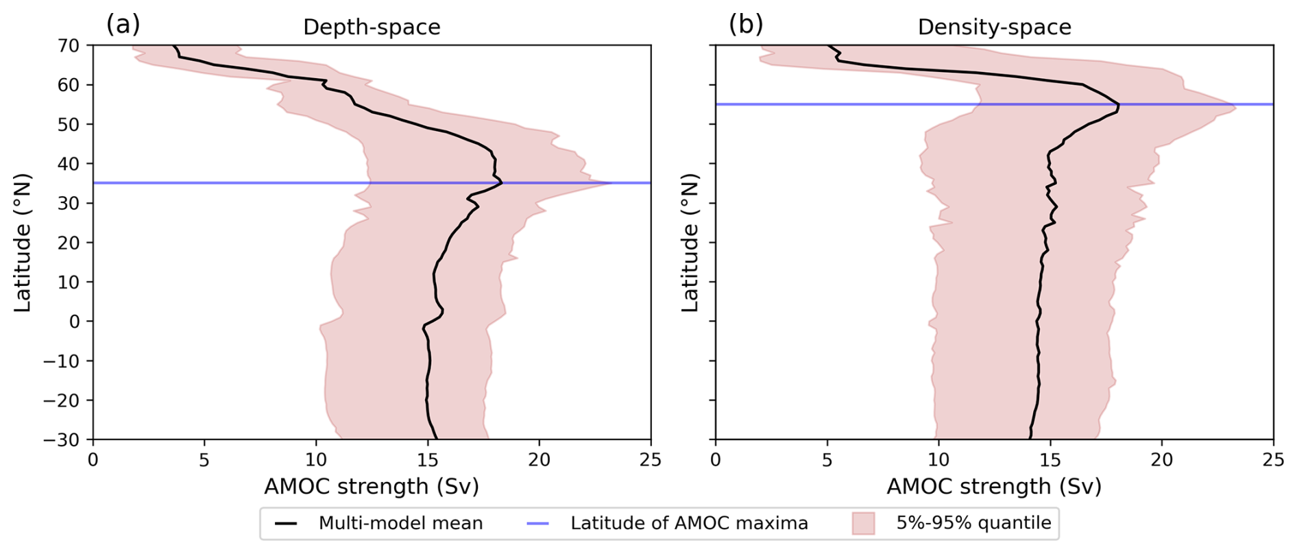
Figure 1 Average AMOC strength over the historical period 1850–1899 for depth-space (a) and density-space (b) as a function of latitude. Black lines show the multi-model mean. The blue lines highlight the latitude of the MMM streamfunction maximum. The red shading shows the 5 %–95 % quantile range of the reference strengths for the model set. Note the substantial drop in AMOC strength north of 65° N in both representations.

AMOC strength is calculated as a 10-year running mean from 1900–2100 for the historical and four future scenarios labelled at the centre year of the decade, providing “annual” AMOC strengths from 1905–2095. The percentage weakening is computed relative to the reference period at each latitude. Latitudes are resampled onto a regular 1° resolution grid from 30° S to 65° N for consistency across the models. Changes to the streamfunctions north of 65° N are not considered due to the weak mean streamfunction and curved model grids at these latitudes.

AMOC weakening refers to the reduction in AMOC strength relative to the reference period. Thus, a negative AMOC weakening indicates a strengthening of the AMOC relative to the reference period. The use of percentage weakening rather than absolute reduction (in Sverdrups) is to allow the direct comparison of weakening between models that have a wide range of AMOC strengths, as is evident in the quantile ranges seen in Fig. 1. The use of percentage normalisation does not remove potential method-dependent structural differences between models of underlying AMOC diagnostics.

Taken at the multi-model mean peak (35° N for depth-space, 55° N for density-space), AMOC strength ranges from 10.7 Sv (IPSL-CM6A-LR) to 23.8 Sv (TaiESM1) and from 11.5 (CanESM5) Sv to 24.7 Sv (TaiESM1) for depth- and density-space respectively. To provide context on our model set in relation to the wider literature, we calculate the AMOC decline at 26° N for ssp585 using the method described in Weijer et al. (2020) to compare mean weakening of the two different model sets. That paper takes the historical reference over the entire historical period (1850–2014). The model set for this paper has a mean percentage weakening of 45 %, where MRI-ESM2-0 has the most weakening at 67 % and EC-Earth3 is at the low end with 27 % weakening (Fig. C1). This is larger than the mean weakening of 39 % found in the aforementioned study. Our model set skews slightly towards models with greater AMOC weakening.

2.4 Threshold Weakening

To connect AMOC weakening across latitudes, contours are computed at specific percentages of weakening, henceforth referred to as weakening thresholds or threshold. The first year a given weakening threshold is exceeded is recorded at each latitude. The threshold line is defined for a specific weakening threshold, e.g. 15 %, as the contour of years as it changes across latitudes. The latitude at which the threshold is first exceeded indicates the year where AMOC weakening originates. The weakening anomaly of a given threshold can be followed throughout the basin to reveal its propagation. The threshold lines are calculated at 2.5 % intervals over the range 2.5 %–60 % between 2000-2095.

The gradient of the threshold line (here-on referred to as the “weakening gradient”) represents the speed of propagation of the AMOC weakening signal at a specific percentage reduction. The larger the weakening gradient, the faster the signal is transported southward. Assuming the threshold lines are approximately linear, the weakening gradient is found by performing a linear least-squares regression between 40° N and 30° S. This latitude range is chosen to capture the propagation south of the weakening onset. To ensure confidence in the validity of the gradient for a given threshold there must be at least a continuous line of thresholds from 40° N to the equator. This prevents erroneous gradients arising from limited data points. With these criteria, the linear fits of all models have a mean p-value < 0.05 (Fig. C2). All models, with the exception of ACCESS-ESM1-5 and EC-Earth3, have a mean absolute r-value > 0.8 for all four scenarios (Fig. C3).

The use of a rolling decadal mean is essential to the functioning of the first exceedance framework used to calculate thresholds. Without it, interannual variability would dominate the threshold lines and present a very noisy dataset, significantly lowering confidence in the linear fit and onset years. As we are interested in the mean state change of the AMOC and not in the propagation of annual and sub-decadal anomalies, our use of a rolling decadal mean is justified.

When comparing differences between future scenarios, the significances are computed using a two sided student t-test and a p-value of 0.05.

3 Results

The results are presented in three sections: differences in AMOC weakening between the depth-space and the density-space representation in the ssp585 experiment (Sect. 3.1), comparisons of weakening across four ScenarioMIP experiments (Sect. 3.2) and different weakening behaviours across the CMIP6 models used in this study (Sect. 3.3).

3.1 Depth-space and density-space

The MMM reference streamfunctions for depth-space (Figs. 1a and 2a) and density-space (Figs. 1b and 2b) respectively show peak overturning at 35 and 55° N. By the end of the 21st century both streamfunctions have shoaled and weakened in amplitude (Fig. 2c and d). The streamfunction maxima are now at 30° S for both representations and there is no longer a clearly defined latitudinal maxima in the North Atlantic. Taking the difference between the reference streamfunction and the ssp585 streamfunction confirms that the greatest reduction in the AMOC occurs where the AMOC is strongest in the reference (Fig. 2e and f). Figure 2f also shows an increase in the density-space streamfunction at the lightest densities north of 40° N. This increase is due the surface waters in the SPG becoming less dense due to subsurface warming (Lin et al., 2023; Levang and Schmitt, 2020), so it is not that the streamfunction has strengthened but instead the density classification has shifted. The standard deviations of the differences in the model ensemble reveal that the largest model spread is not aligned with maximum weakening (Fig. 2g and h). Instead, the greatest standard deviations are on the contours above and below the peak. This could indicate the model spread is most strongly determined by the intensity of shoaling and change in vertical position of the AMOC streamfunction as it weakens. This relates to a recent study that found models with deeper AMOCs exhibit greater shoaling than with shallower AMOCs and these models with deeper AMOCs may be more sensitive to warming than observations imply (Bonan et al., 2025).

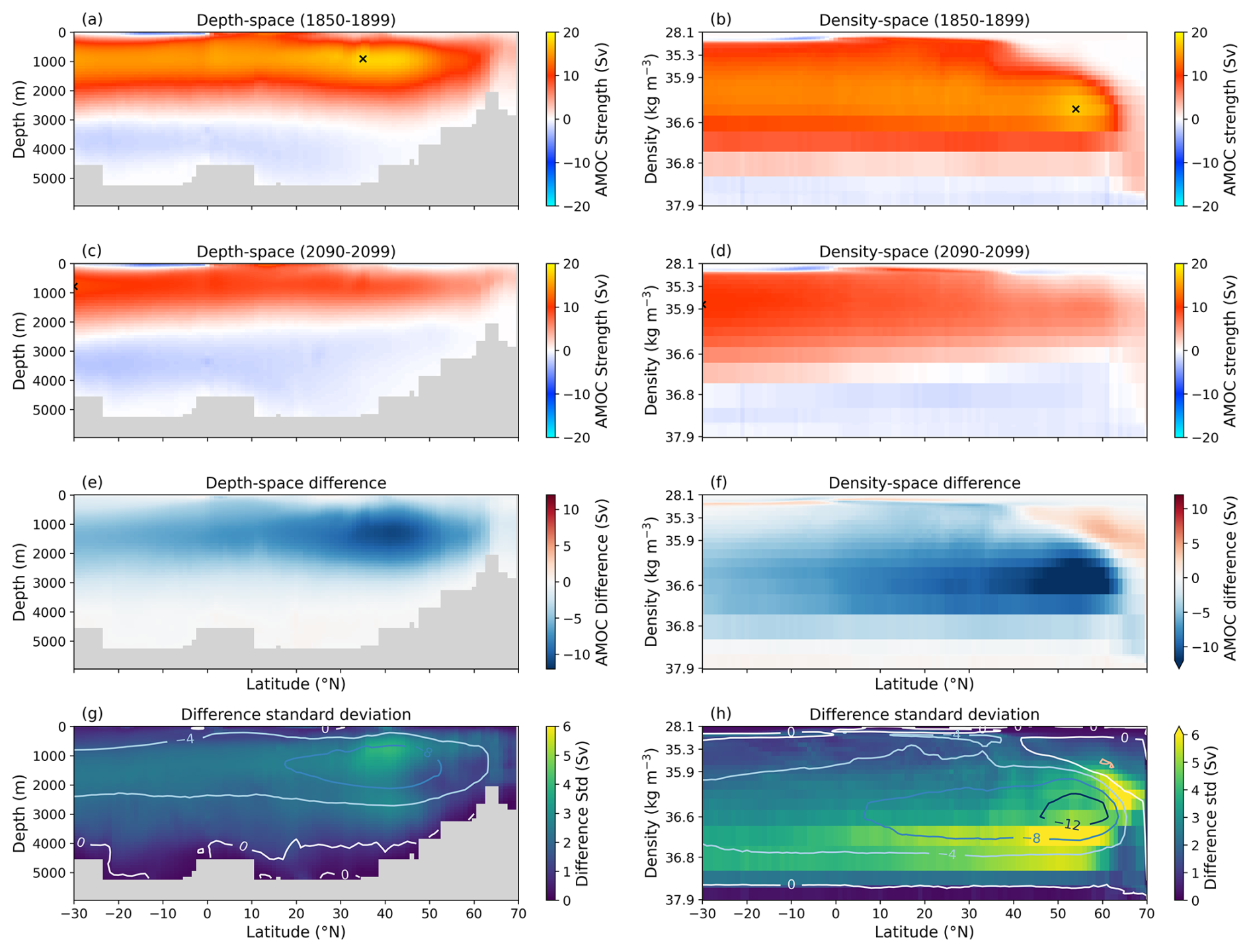
Figure 2 Multi-model mean depth-space (left column) and density space (right column) streamfunctions. (a, b) Averaged over the historical reference period (1850–1899). (c, d) Averaged over the last decade of the ssp585 scenario (2090–2099). The maxima of the streamfunctions are marked by “x”. (e) The difference between (a) and (c). (f) The difference between (b) and (d). (g, h) the standard deviations of the differences (e, f) contoured with the differences. Note the non-linear vertical scale in the density plots. Topography in depth-space is the aggregation of all model topographies.

By representing AMOC weakening as a function of latitude and time, the connectivity of AMOC weakening across the Atlantic basin is revealed and the timescales of AMOC weakening can be inferred. Figure 3 shows the percentage weakening Hovmöllers for depth-space and density-space plots from the first decade after the reference period (1905) to the end of the ssp585 experiment (2095). Changes from 1905–2000 are not of particular interest to this study but are included for completeness. This time period does show AMOC strengthening between 1960–2000 of approximately 10 % in both depth and density space, attributed to aerosol emissions (Menary et al., 2020), before the AMOC starts declining from 2015.

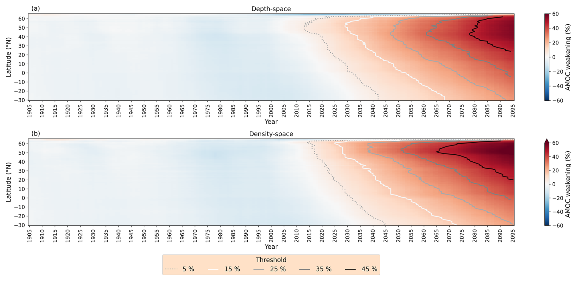
Figure 3 Multi-model mean Hovmöller plots of percentage AMOC weakening for (a) depth-space and (b) density-space over the historical (1905–2014) and ssp585 (2015–2095) experiments, relative to the historical reference period (1850–1899). AMOC weakening is taken as a rolling decadal average. Threshold lines of 5 %, 15 %, 25 % 35 % and 45 % weakening are shown.

AMOC weakening begins at high latitudes, north of 40° N, with a weakening signal propagating to the southern boundary of the Atlantic basin in both depth-space and density-space (Fig. 3a and b). This is clearest when following the threshold lines. At the 5 % threshold, the time to traverse from the latitude of onset to 30° S is approximately three decades (2015–2045). At the 25 % threshold, this takes ∼ 45 years for depth-space and ∼ 55 years for density-space. Density-space has a longer signal than depth-space because the latitude of onset is further north in density-space than depth-space. This might be expected when looking at the streamfunctions (Kwon and Frankignoul, 2014), as the density streamfunction takes into account changes in the zonal structure in higher latitude North Atlantic, which are suppressed in the depth-space streamfunction and the maximum of the density-space streamfunction is likewise further north than the depth-space streamfunction. In both depth and density space representations of the AMOC streamfunction, there is a southward shift of the onset latitude as the threshold increases, 51 to 45° N in depth-space and 61 to 51° N in density-space from 5 % threshold to 45 % threshold. The difference between onset latitudes means density-space shows AMOC weakening earlier than in depth-space. For example, the 25 % threshold reached in 2035 in density-space compared to 2047 in depth-space. South of 40° N the timings of the threshold lines realign between the two representations. That AMOC weakening begins in the north suggests methods for early warning signals should focus more on high latitude monitoring.

Relating Fig. 3 to the latitudes of the observational arrays RAPID (26° N, Smeed et al., 2014) and OSNAP (53–60° N, (Lozier et al., 2017), where we use 57° N to represent the whole array) reveals that for thresholds over 10 %, weakening at OSNAP leads weakening at RAPID by at least a decade (10–22 years, the range increases as threshold increases) in density-space while only precedes by 4–11 years in depth-space. As an illustrative example, we consider the difference in detection time of 25 % weakening at OSNAP and RAPID in depth-space and density-space. In density-space, OSNAP precedes RAPID by 17 years for ssp585 (ranging over 17–21 years, depending on scenario). In depth-space, OSNAP precedes RAPID by only 5 years for ssp585 (ranging over 4–8 years, depending on scenario). Since the onset latitudes of AMOC weakening in depth-space are further south than the OSNAP array, there are delays in detection at OSNAP when compared to the detection of weakening in density-space, where the onset latitudes broadly overlap the OSNAP latitudes. Depth-space performs better for early warning when measured at the latitude of most intense weakening (∼ 45° N) to 26° N. For 25 % weakening, depth-space weakening at 45° N precedes 26° N by 8 years for ssp585 (ranging over 8–15 years, depending on scenario). Density-space still generally outperforms along this latitude range, with a time difference of 11 years for 25 % weakening in ssp585 (ranging over 11–16 years, depending on scenario) and still has the additional signal from further north (8 years for 25 % weakening in ssp585). For less than 10 % weakening, depth-space signal precedes the density-space signal by 0–7 years. This is likely due to the high latitude (40–60° N) weakening between 2000–2015 that is seen in depth-space and not density-space.

The timescales associated with the weakening gradients found are longer than the propagation timescales of density anomalies (e.g. Zhang, 2010; Hodson and Sutton, 2012), however they do align with timescale of some studies on AMOC adjustment to high latitude forcing (Kwon and Frankignoul, 2014; Gerdes and Köberle, 1995; Döscher et al., 1994). This will be discussed further in Sect. 4.

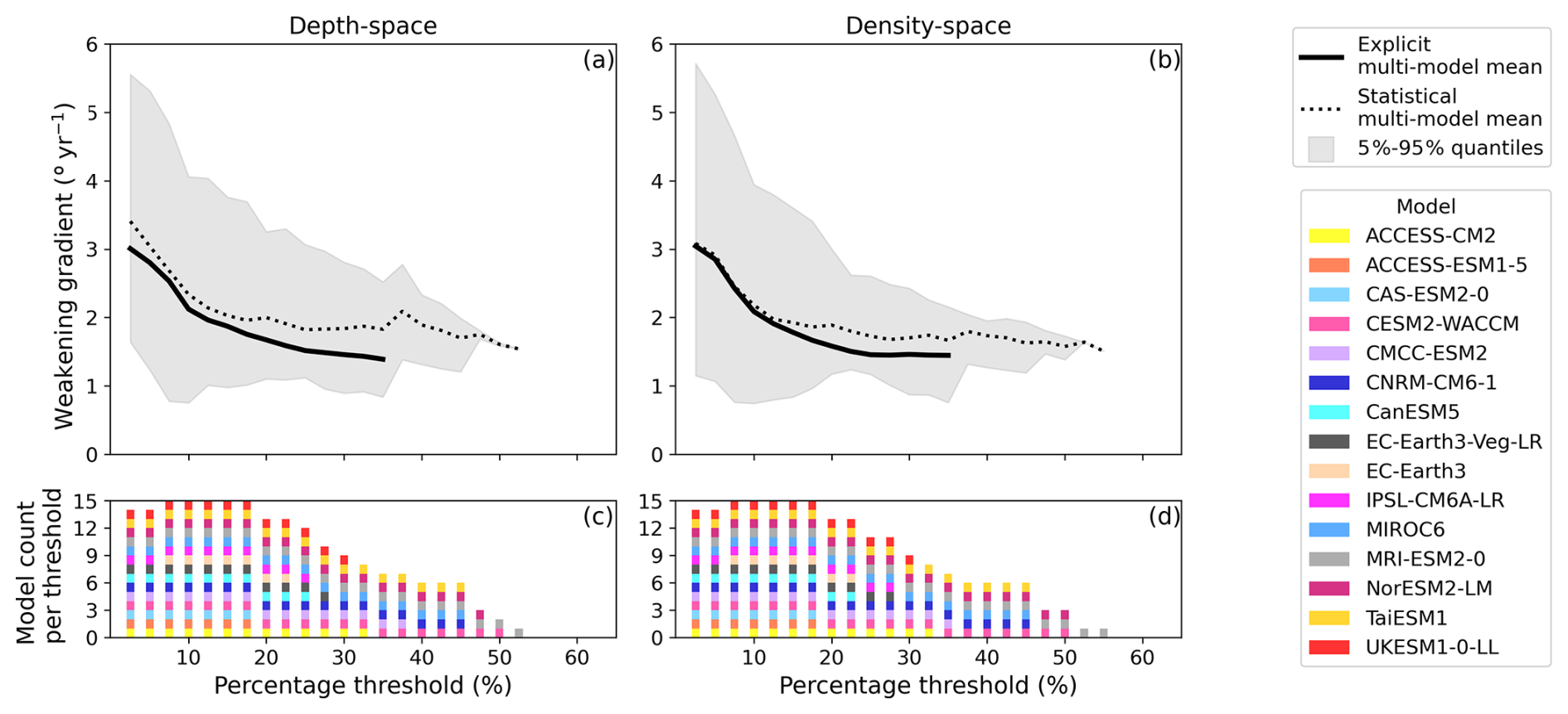
Figure 4 The weakening gradient of the threshold lines (between 40° N and 30° S) at 2.5 % intervals for (a) depth-space and (b) density-space. The continuous black line are the weakening gradients of multi-model mean threshold lines, as seen in Fig. 3. The dotted black line is the statistical multi-model mean, calculated from the individual weakening gradients of the model set, and the red shading is the 5 %–95 % quantile range of the model set. (c, d) The models included for the statistical calculations at each threshold. The speed of the weakening gradient is measured in degrees per year.

For the multi-model set, weakening gradients are calculated for each model and each scenario and are calculated in the unit degrees per year (° yr⁻¹). There are two approaches for considering the MMM weakening gradients.

Method 1: Calculating weakening gradients of the MMM Hovmöller threshold lines (seen on Fig. 3). We call this the explicit multi-model mean (EMMM) (Fig. 4a and b, solid black line).

Method 2: At each threshold, computing the weakening gradient of each model individually before taking the mean across all the models. This does not include the MMM Hovmöller threshold lines. We call this the statistical multi-model mean (SMMM) (Fig. 4a and b, dotted black line).

All the models in the model set contribute to all the values of the EMMM weakening gradients whereas since the SMMM weakening gradients are calculated separately at each threshold, the number of models involved can vary (Fig. 4c, d). Analysis will primarily focus on the EMMM weakening gradients with the SMMM weakening gradients and associated 5 %–95 % quantiles acting as a reference for the behaviour of the model set.

For both depth-space and density-space, there is a gradual reduction of the EMMM weakening gradient ending in a plateau starting at around the 25 % threshold as the threshold increases. The EMMM weakening gradient reduces from 3.01 to 1.39° yr⁻¹ for depth-space and 3.04 to 1.45° yr⁻¹ for density-space, i.e. in both representations the weakening gradient has halved and, by proxy, we infer the propagation speed of weakening has halved. The story is similar for the SMMM weakening gradient, although the gradients are consistently slightly higher (by an average of 0.28° yr⁻¹) and due to a handful of models with weakening gradients at high thresholds, the SMMM weakening gradients persist along higher thresholds. The SMMM weakening gradients at high threshold should be considered cautiously, since the number of models contributing to statistical calculations are diminishing (Fig. 4c, d). The model missing at the 2.5 % and 5 % threshold is EC-Earth3 as this model starts the century more than 5 % weaker than its historical reference, and weakening gradients cannot be calculated at these thresholds.

The interpretation of changes to weakening gradients seen in Fig. 4 is that as the AMOC weakens there is a gradual slowdown in the southward speed of propagation of AMOC weakening, down to a minimum, constant propagation speed. This is consistent in both depth and density space analysis.

Figure 4 shows an intriguing reduction of the weakening gradient as the AMOC weakens but also poses three questions: (1) Do all future projection scenarios have similar weakening gradients? For example, does a 25 % reduction in the AMOC propagate at the same speed across the Atlantic basin regardless of specific forcing? (2) Do individual models follow the same gradient curve as the EMMM? (3) Why does the gradient slow at lower thresholds and plateau at higher thresholds?

The next section (Sect. 3.2) will address the first question and Sect. 3.3 will address the second question while the third question will be a topic of discussion.

The differences between depth and density-space have been explored in this section. While there are differences between the high latitude response to AMOC weakening in depth-space and density-space, the behaviour in weakening gradients south of 40° N is comparable between the two representations. As density-space reveals more details of high latitude processes than depth-space and is more descriptive for AMOC propagation in connection to those high latitudes (Zhang, 2010; Kwon and Frankignoul, 2014), the remainder of the analysis will be presented using the density-space representation. This will capture a more complete representation of AMOC weakening than depth-space. There is very little difference between depth and density space and the equivalent figures for depth-space have been included in Appendix E.

3.2 The ScenarioMIP experiments

This section explores differences in density-space AMOC weakening between the future scenarios; ssp126, ssp245, ssp370 and ssp585.

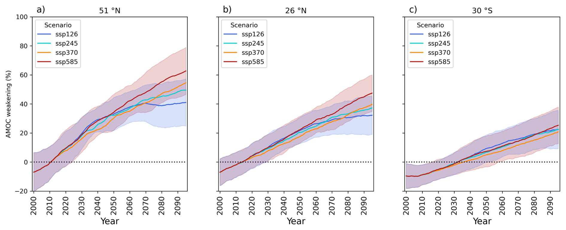
Figure 5 Timeseries of MMM AMOC weakening for the four scenarios relative to the 1850–1899 reference at (a) 51° N, (b) 26° N and (c) 30° S. Red and blue shading show 1 SD for ssp585 and ssp126, respectively.

To initially assess differences between scenarios, timeseries of AMOC weakening are shown for 3 selected latitudes of 51° N, 26° N and 30° S (Fig. 5). As was inferred from Fig. 3, the rate of AMOC weakening is greatest at high latitudes (51° N) and is slower at lower latitudes (26 and 30° S). The latitude with the greatest divergence in AMOC weakening between scenarios is 51° N with end of century MMM weakening of 63 % in ssp585 and 41 % in ssp126 but also the largest standard deviations for those two experiments of the latitudes (Fig. 5a). In contrast, end of century weakening at 26° N is 47 % in ssp585 and 32 % in ssp126 (Fig. 5b) and at 30° S is 25 % in ssp585 and 22 % in ssp126 (Fig. 5c). AMOC weakening is more responsive to climate forcing in northern latitudes than latitudes further south. For example, under ssp585 forcing 25 % weakening is reached in 2036 at 51° N, 2055 at 26° N and only in 2095 weakening at 30° S. The latitudinal responsiveness can also be seen when looking at “negative” weakening (when the AMOC has elevated strength relative to the reference). The two higher latitude figures show weakening start by 2015, whereas at 30° S it takes until the mid 2030s (depending on scenario) to start experiencing positive weakening. The divergence between scenarios appears mainly driven by a slowdown of weakening in the lower emissions scenarios (ssp126 and ssp245) as the rate of weakening for ssp370 and ssp585 appears largely unchanged over each timeseries. A point of interest is that the AMOC weakening for ssp370 is consistently less than the other three experiments until the mid-2060s, contrary to the expectation that higher emissions scenarios lead to greater AMOC weakening but by the end of the century the amplitude of weakening in each scenario corresponds to the severity of the emissions in that scenario. The AMOC weakening being less for ssp370 is a consistent feature across the model set. Another point of interest with ssp370 is that it has a slower rate of weakening to the other scenarios prior to 2050, in disagreement with what was found by Weijer et al. (2020). This may be due to differences in the method of calculating the timeseries, such as this use of percentage difference taking the rolling decadal average rather than rolling annual average, or because our study uses a smaller number of ensemble members than their study used.

Relative to the 1850–1899 reference period, the AMOC is shown to already be weakening from the year 2000 at 51° N (Fig. 5a) and 26° N (Fig. 5b), which is model dependent and due to the model's sensitivity to aerosols (Robson et al., 2022). While the RAPID array has not yet detected significant weakening across 2004–2022 (Jackson et al., 2022), statistically significant weakening has been seen in specific water masses after decomposing the AMOC (e.g. in the deep western boundary) (Pita et al., 2026). Observational arrays are subject to large internal variability which could obscure AMOC weakening (McCarthy et al., 2025). Longer timescales of observations are required to detect any weakening of the real-world AMOC, with Lobelle et al. (2020) proposing at least 29–67 years of RAPID observations to be at the 90 % confidence level of detection, but decomposing the AMOC as was done by Pita et al. (2026) could reduce this timescale. Weakening has not yet been significantly observed by OSNAP (2014–2021) (Li et al., 2021).

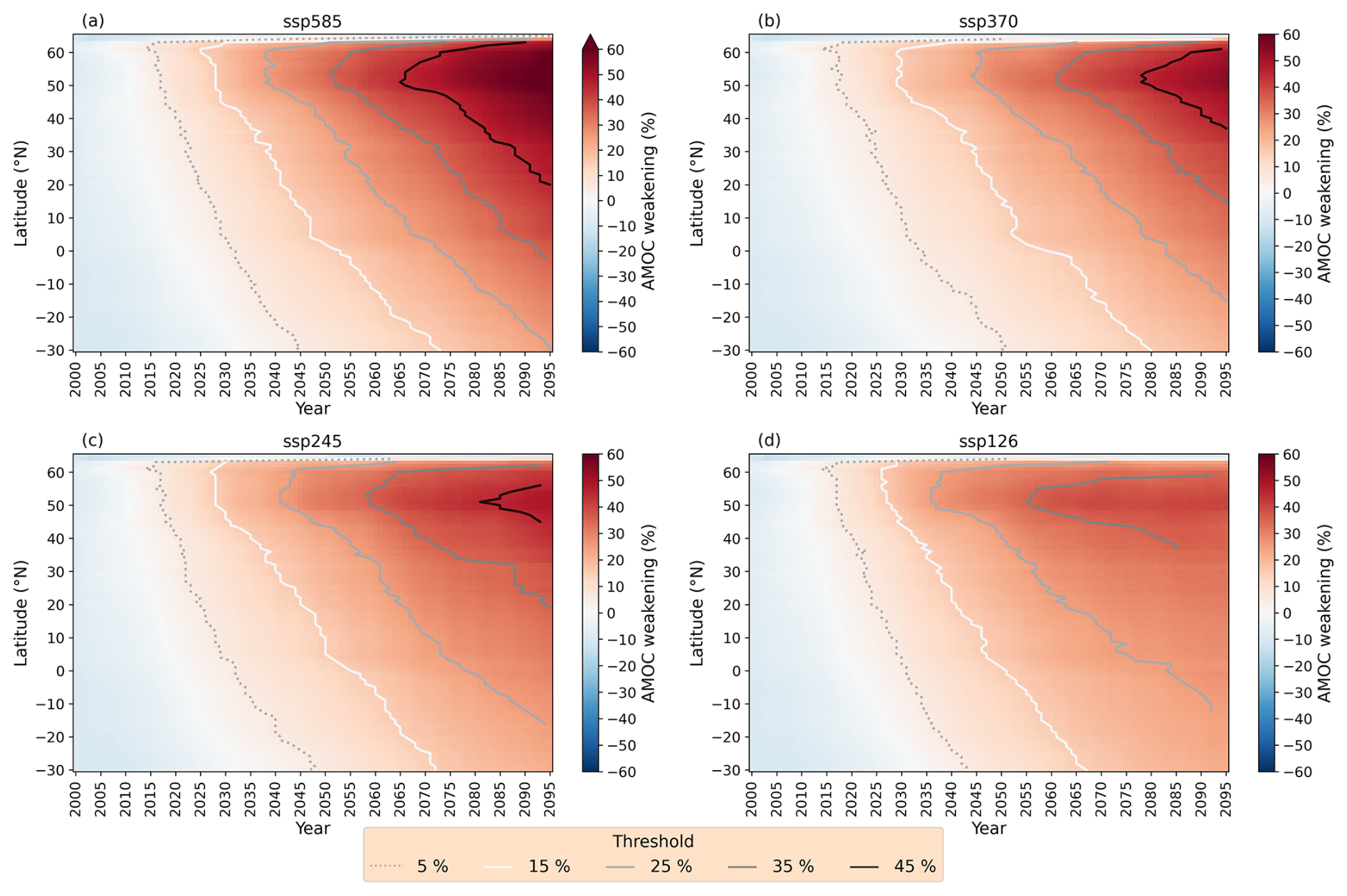
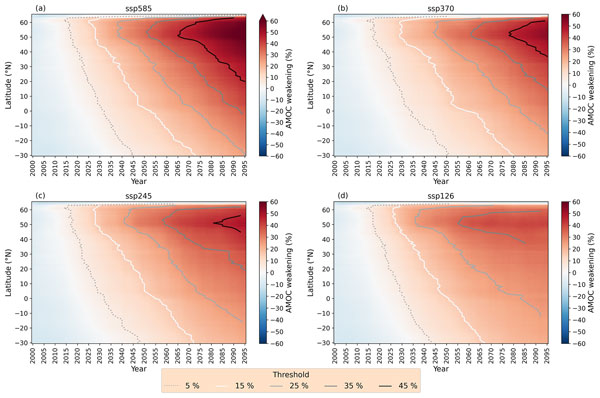
Figure 6 Multi-model mean weakening Hovmöller plots for the four ScenarioMIP scenarios (2000–2095) in density-space. Scenarios are (a) ssp585, (b) ssp370, (c) ssp245, (d) ssp126. Threshold lines of 5 %, 15 %, 25 %, 35 % and 45 % are shown where they exist. (a) is as seen in Fig. 3b, reproduced here for ease of comparison.

Having assessed AMOC weakening at specific latitudes, we now consider the full basin response to AMOC weakening for the four scenarios. All scenarios exhibit positive weakening gradients, indicative of a north-to-south propagation of AMOC weakening (Fig. 6) with weakening onset occurring at high latitudes similar to what was shown for ssp585 in Sect. 3.1. At a glance, Hovmöller plots are broadly similar for the first 50 years with similar threshold lines of 5 % and 15 % weakening after which the scenarios start diverging with ssp585 experiencing the greatest weakening and ssp126 experiencing the least. Detailed comparisons between scenarios are found by taking pairwise differences of the four Hovmöller plots, testing for 95 % significance of difference found with a student t-test (Fig. 7).

Considering the scenarios compared to ssp585, the greatest magnitude end of century differences are with ssp126 (Fig. 7a), with smaller differences for ssp245 (Fig. 7b) and smaller again for ssp370 (Fig. 7c), consistent with Fig. 5. Interestingly, there are hardly any significant differences between ssp585 and either ssp126 or ssp245 before 2050. When the differences do become significant they do not propagate at the speed of the weakening gradients but can occur over a large range of latitudes in a single year and at least for the case with ssp245, it appears the equator may present a barrier for differences to propagate across (Fig. 7b). This is not seen in Fig. 7c, as the ssp370 and ssp585 are significantly different for the vast majority of the basin and time period because at every latitude AMOC weakening for ssp370 is less rapid than for ssp585 (Fig. 5).

The remaining pairwise differences between emissions scenarios (ssp126, ssp245 and ssp370) are characterised by less extreme emissions scenarios experiencing greater weakening than the more extreme emissions scenarios, especially before 2070 (Fig. 7d–f). This is contrary to what we expect from the end of the century, and indeed after 2070 this trend is reversed, especially north of 50° N. In comparisons with ssp370, significant differences south of the equator persist until the 2090s. Comparing similar experiments (ssp370 and ssp245, Fig. 7e) and (ssp245 and ssp126, Fig. 7f), there are wavelike periods with no significant differences in AMOC weakening possibly driven by multi-decadal variability aligning AMOC strengths. Figure 7d and f also show an indication that the equator is a barrier for differences to cross.

The ssp370 scenario has been shown to be consistently different from the other scenarios (Fig. 7c–e) and with a different rate of reduction of weakening (Fig. 5). This scenario is characterised by high aerosol emissions, which have been linked with strengthening the AMOC (Menary et al., 2020). The increased presence of aerosols in the atmosphere may explain the slower weakening of the AMOC in this scenario.

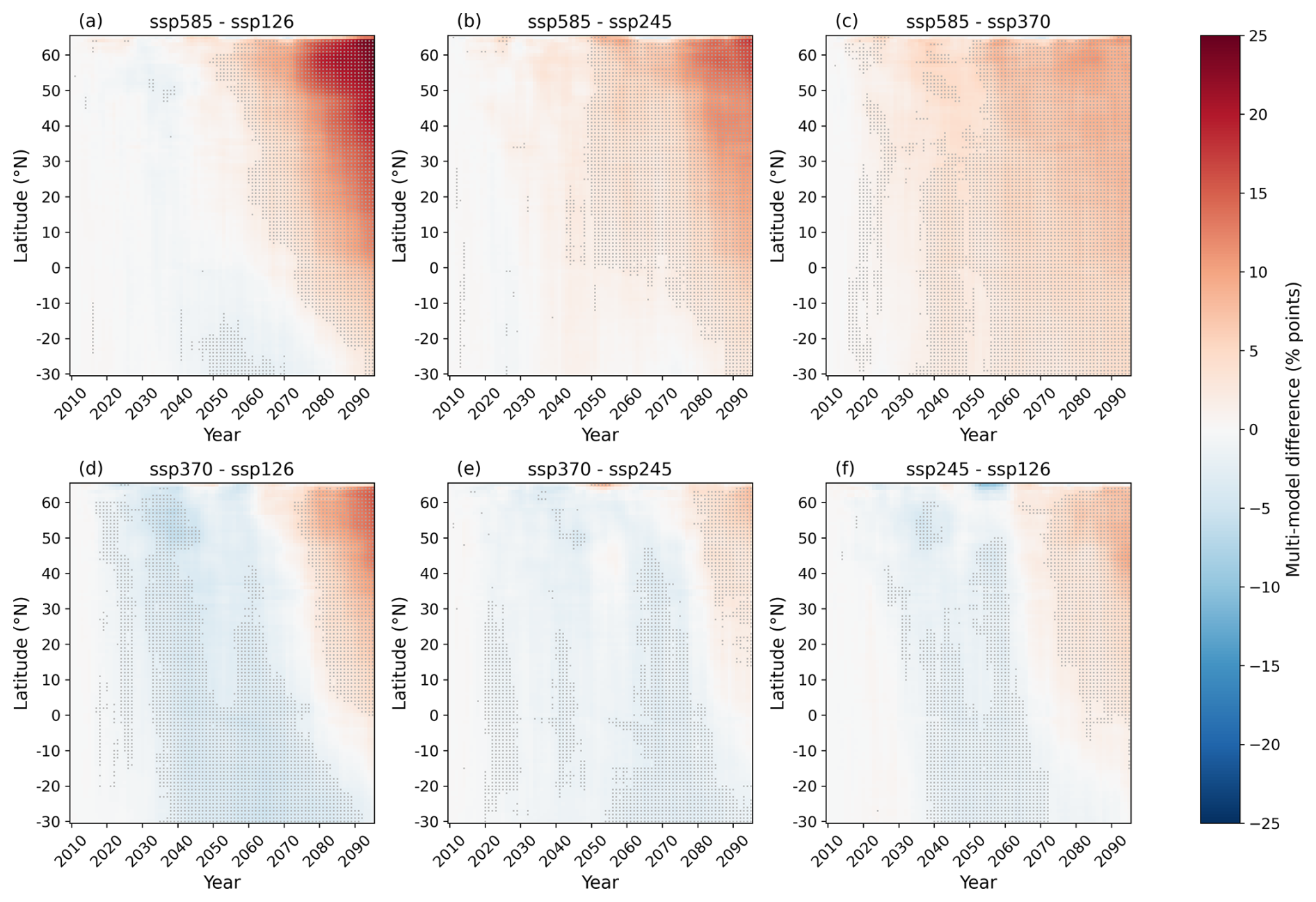
Figure 7 The pairwise differences of AMOC weakening between the four ScenarioMIP experiments. Weakening in the more extreme emissions scenario is subtracted by weakening in the less extreme emissions scenario. Positive (red) means the more extreme emissions scenario has greater weakening, negative (blue) means the less extreme emissions scenario has greater weakening. 95 % significance from a student t-test is indicated by a dot.

Figure 7 explores the magnitude and spatial distribution of differences in AMOC weakening between scenarios but to understand differences in latitudinal connectivity we must return to Fig. 6. At high threshold (≥ 25 %) the threshold lines in the lower emissions scenarios reduce in gradient, southward propagation is slower, while in higher emissions scenarios there isn't such a noticeable change in the threshold line gradient (Fig. 6). The reduction in weakening gradient for lower emissions scenarios is clear in Fig. 8 as is the relatively constant propagation speed in the high emissions scenarios. In Fig. 8, both ssp126 and ssp245 show a continuous reduction in weakening gradient as threshold increases while for ssp370 and ssp585 the weakening gradient initially reduces but plateaus at high thresholds. The EMMM weakening gradient for ssp370 also starts lower than any of the other experiments with the 2.5 % threshold gradient at 2.50° yr⁻¹ compared to 2.99° yr⁻¹ (ssp585), 2.92° yr⁻¹ (ssp245) and 3.04° yr⁻¹ (ssp126), further supporting its uniqueness from the other experiments.

The plateau of high threshold weakening gradient could indicate a minimum speed of propagation in response to strong forcing that is not required for weaker forcing. Alternatively, depending on the mechanism for southward propagation of weakening is, if the driver of weakening stops or slows in lower emissions scenarios, it is plausible that the southward progression of a weakening signal would stop or slow as well. Figure 5 shows that the rate of AMOC weakening varies as a function of latitude. The process that sets the rate of weakening at a fixed latitude is not the object of this study but we posit is strongly related to the propagation of AMOC anomalies through the basin. Exactly understanding the mechanism that propagates weakening southward would provide insight into this slowdown across the scenarios. Does weakening in the high latitudes and SPG necessitate weakening for the rest of the AMOC?

Figure 8 Density-space weakening gradients, as seen for ssp585 in Fig. 4, for all four ScenarioMIP experiments. (a) ssp585, (b) ssp370, (c) ssp245, (d) ssp126 and (e–h) the models used for the SMMM and quantile calculations. (a) is as seen in Fig. 4, reproduced here for ease of comparison.

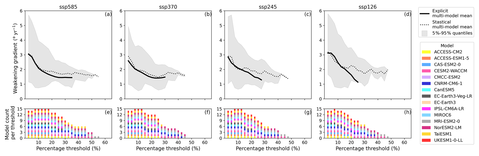
Figure 8c and d show a divergence between the EMMM line and the SMMM line, where the SMMM plateaus rather than continuously declining. This is a surprise, but considering the number of models involved in the high threshold statistics (Fig. 8e-h), this divergence only occurs between the multi-model mean and a small number of models. As will be shown in Sect. 3.3, most models show similar behaviour to the EMMM rather than the SMMM.

3.3 Inter-model comparison

This section explores intermodel behaviour of AMOC weakening. We primarily focus on the subset of models with multiple ensemble members: CNRM-CM6-1 (6), CanESM5 (16), IPSL-CM6A-LR (3), MIROC6 (3) and UKESM1-0-LL (5), with numbers in the brackets indicating the number of ensemble members. We focus on these models to reduce the uncertainty associated with internal variability. We also present three models with only one ensemble member (MRI-ESM2-0, NorESM2-LM and TaiESM1) to highlight weakening gradient behaviours not seen in the ensemble analysis.

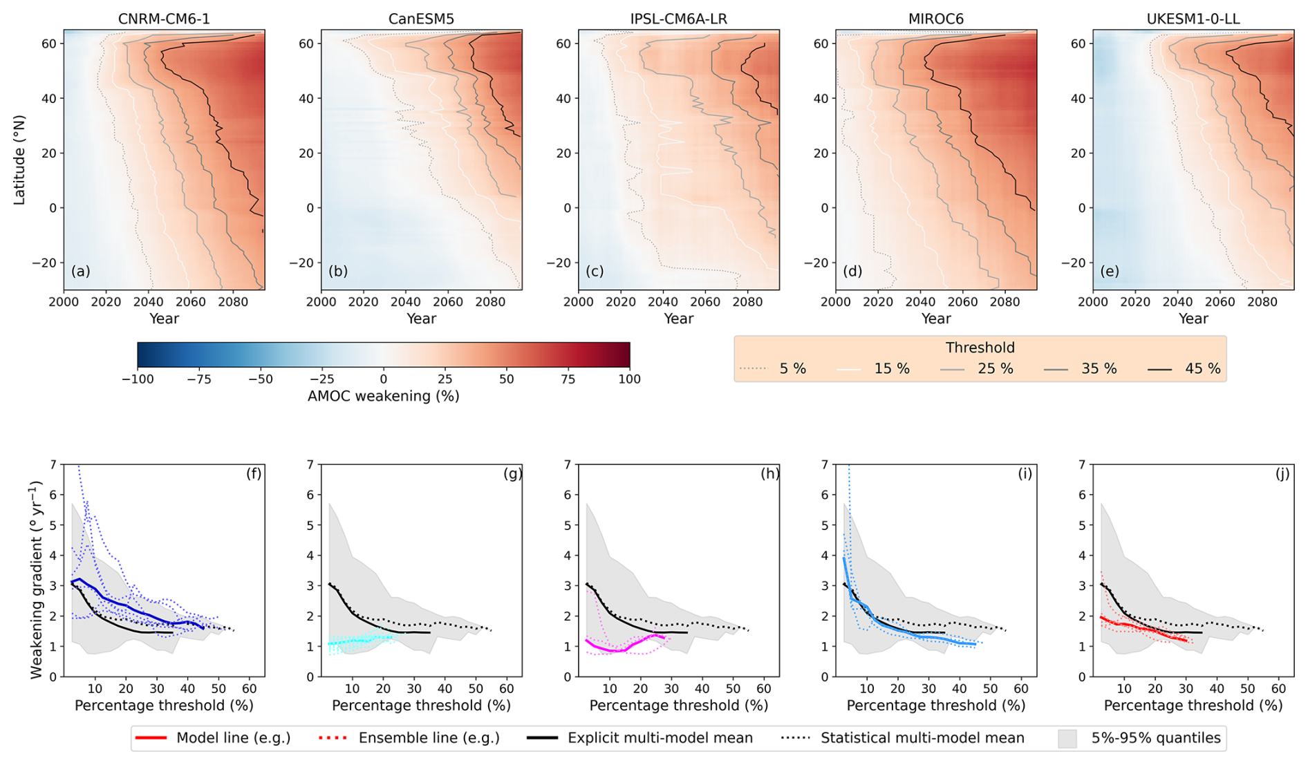
Figure 9 AMOC weakening in density-space for the model subset with multiple ensemble members for ssp585. (a–e) Individual model Hovmöller plots shown with threshold lines of 5 %, 15 %, 25 %, 35 % and 45 % reduction. (f–j) Individual weakening gradient plots imposed over the multi-model mean gradient and statistics. The model lines are the weakening gradients found from the ensemble-mean Hovmöller. Hovmöller and weakening gradient plots of the full model set can be found in Appendix D.

The ensemble mean Hovmöller for ssp585 generally show smoother and less variable behaviour than their individual ensemble members (Figs. 9a–e and D5). Likewise, the weakening gradient of the ensemble means are also less variable than their individual ensemble counterparts, especially CNRM-CM6-1 (Fig. 9f–j, model and ensemble lines). The speed of weakening gradients is visibly model dependent, with some models faster (e.g. CNRM-CM6-1) and some slower (e.g. CanESM5), especially when compared to the EMMM and SMMM lines.

CNRM-CM6-1, MIROC6 and UKESM1-0-LL show that as the AMOC weakens, the weakening gradient also reduces (Fig. 9f, g and j). This is the same trend as the EMMM and SMMM. MIROC6 shows similar behaviour to the MMM lines having a non-linear decrease with increasing threshold. The final weakening gradients are 1.06° yr⁻¹ for MIROC6 at 45 % weakening, 1.45° yr⁻¹ for the EMMM at 35 % weakening and 1.51° yr⁻¹ for the SMMM at 55 % weakening.

Unlike the non-linear reduction shown by MIROC6, CNRM-CM6-1 and UKESM1-0-LL have a more linear reduction in weakening gradient, with CNRM-CM6-1 declining from 3.13° yr⁻¹ at the 2.5 % threshold to 1.58° yr⁻¹ at the 45 % threshold (Fig. 9f) and UKESM1-0-LL declining from 1.95° yr⁻¹ at the 2.5 % threshold to 1.18° yr⁻¹ at the 30 % threshold (Fig. 9j). These amount to a 50 % reduction in weakening gradient for CNRM-CM6-1 at the 45 % threshold and a 39 % reduction in weakening gradient for UKESM1-0-LL at the 30 % threshold. While the ensemble means of these two models show a linear reduction, the UKESM1-0-LL ensemble lines are similar to the ensemble mean whereas CNRM-CM6-1 shows a range of values spanning the 5 %–95 % quantiles of the model set. CNRM-CM6-1 has been shown to have greater internal variability than the other models in this set (Coquereau et al., 2026) which may explain the large range of ensemble member weakening gradient behaviours.

CanESM5 is a model with particularly low weakening gradients compared to the model set (see Appendix D, Fig. D3) and differs from the MMM weakening gradient behaviour. It is the model with the greatest number of ensemble members in our analysis (16) and the ensemble spread in weakening gradients is small relative to other models (Fig. 9g). The ensemble mean weakening gradient at the 2.5 % threshold is 1.08° yr⁻¹ which gently increases to 1.29° yr⁻¹ at the 22.5 % threshold (Fig. 9g). This is a near constant weakening gradient in comparison to the MMMs.

Of the five models in the model subset, IPSL-CM6A-LR has the most unclear weakening gradient behaviour with a decrease in weakening gradient followed by an increase (Fig. 9h). This behaviour is not inherently physically implausible but it appears more likely to be a limitation of the threshold line method rather than a physical process (Fig. 9c). These limitations are best explored studying the 5 % and the 15 % threshold lines (Fig. 9c). Weakening of 5 % propagates from 40° N to 20° S on the order of 20 years (∼ 2020 to ∼ 2040), similar to MIROC6, but 5 % weakening only occurs at the southern boundary of the Atlantic (30° S) in the 2070s. There is a similar delay in the 15 % threshold line at the equator during 2050–2070. The non-linearity of the southward propagation results in a less robust linear fit, that while still statistically significant, results in a smaller weakening gradient than would be expected when considering other parts of the threshold line. This highlights that weakening gradients are most informative when capturing latitudinally coherent weakening (e.g. the other four models) and does not perform as well when fitting noisy threshold lines. IPSL-CM6A-LR is a model with only three ensemble members and the mean may be more sensitive to internal variability.

The trends of the weakening gradients can be grouped by visual inspection by whether the gradient reduces (CNRM-CM6-1, MIROC6, UKESM1-0-LL), increases (CanESM5) or oscillates (IPSL-CM6A-LR). We sort all 15 models into Table 3. The majority of the models (10 out of 15) have a reducing weakening gradient with increasing threshold (Fig. E3). Of those ten, two of them show a plateau in weakening gradient (CESM2-WACCM and TaiESM1) not seen elsewhere in the ensemble set. Two models have an increasing weakening gradient with increasing threshold (CanESM5 and EC-Earth3). Both are models that started with a small weakening gradient. The remaining three models have neither a distinctly increasing or decreasing weakening gradient with increasing threshold (ACCESS-CM2, IPSL-CM6A-LR, MRI-ESM2-0).

Table 3 CMIP6 models sorted by visual inspection according to the weakening gradients response to ssp585 forcing. The categories are whether the weakening gradient increases, decreases or both increases and decreases with increasing percentage threshold.

Figure 10 The same as Fig. 9 but for three models with only one ensemble each.

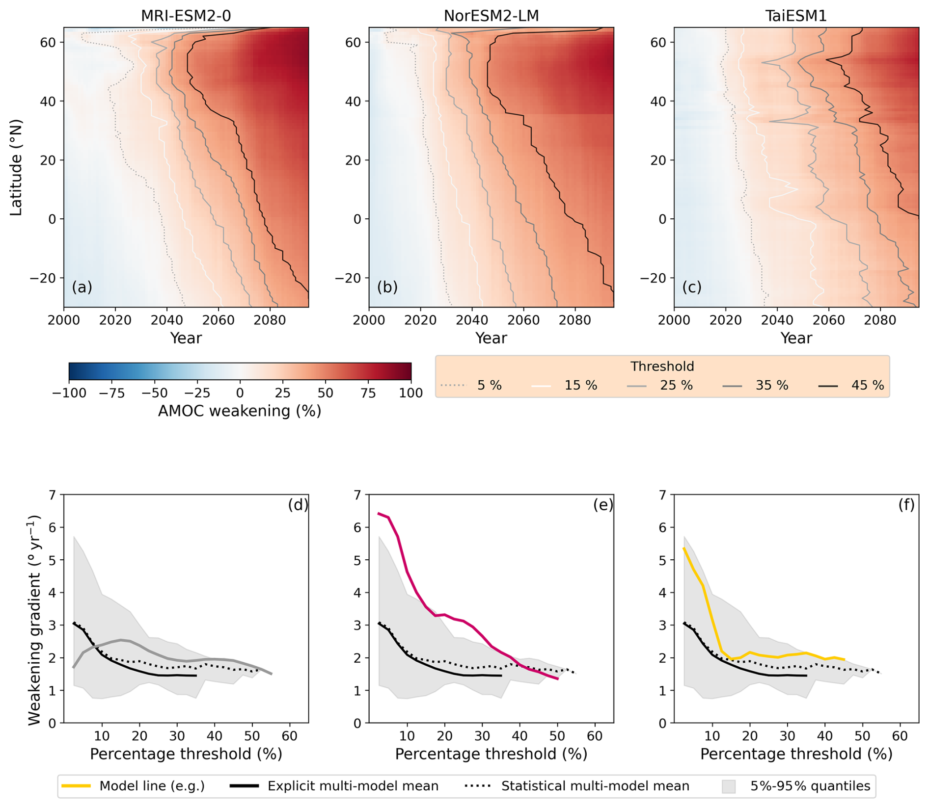
Here we analyse three models (MRI-ESM2-0, NorESM2-LM and TaiESM1) with only one ensemble member that reach a high threshold and are thus visually clearer to analyse (Fig. 10). Ensemble member behaviour can vary substantially (e.g. CNRM-CM6-1) or very little (e.g. CanESM5). With only one ensemble member it is not possible to know if a model will be the former or the latter. For the sake of this analysis, we assume the individual ensemble realisations are representative of the model behaviour but acknowledge that these model results may be due to internal variability.

MRI-ESM2-0 has a somewhat oscillating behaviour, similar to IPSL-CM6A-LR, and does not show a decreasing trend in weakening gradient with threshold (Fig. 10d). MRI-ESM2-0 has a mean weakening gradient of 2.08° yr⁻¹. NorESM2-LM, on the other hand, has a strong decreasing weakening gradient, reducing from 6.41° yr⁻¹ at 2.5 % threshold to a minimum of 1.34° yr⁻¹ (Fig. 10e). This is similar to the the r5i1p1f2 ensemble member of CNRM-CM6-1, meaning this behaviour in NorESM2-LM could be influenced by internal variability, either in the historical reference or the future response. In TaiESM1, instead of a continuous reduction in weakening gradient, there appears to be a two-stage response. Initially there is a rapid, linear reduction until the 15 % threshold from an initial weakening gradient of 5.34° yr⁻¹ which then plateaus to a mean weakening gradient of 2.04° yr⁻¹. If this response is not related to internal variability, it suggests that there is an adjustment period of weakening in future forcing which then settles to a constant speed.

AMOC weakening north of 40° N is not considered in the weakening gradient calculation, but there are interesting features seen in subpolar gyre (SPG) region. CanESM5, IPSL-CM6A-LR and MIROC6 experience noticeable reductions in the SPG region (49 to 63° N) that are not immediately propagated southwards, most pronounced being the delay of the 35 % threshold line (Fig. 9b–d). Meanwhile CNRM-CM6-1 and UKESM1-0-LL show similar behaviour to the MMM with a less clear-cut latitude break (Fig. 9a and e). This indicates high latitude weakening in the streamfunction does not immediately propagate further south. A recent high resolution modelling study (Petit et al., 2025) found that there is a strong relationship between density at OSNAP latitudes with AMOC strength at 45° N but not between AMOC strength at OSNAP latitudes (53–60° N) and 45° N, which aligns with the lack of immediate propagation. However, as is seen in the trio of single ensemble models (Fig. 10), this does not apply to all models. MRI-ESM2-0 and NorESM2-LM show much broader weakening over the SPG region (Fig. 10a and b), displaying greater connectivity between the high and lower latitudes, while TaiESM1 has no visible region of greater weakening (Fig. 10c). The broad weakening response in the SPG for MRI-ESM2-0 and NorESM2-LM cannot just be due to these streamfunctions being provided by modelling centres, as CAS-ESM2-0 (Fig. D5) shows a similar response and is a calculated streamfunction. These models are in disagreement with the results from Petit et al. (2025), but given the differences in experimental set-up and model resolution, it is difficult to assess whether this disagreement has any significance.

Figure 11 The same as Fig. 9 but for ssp126.

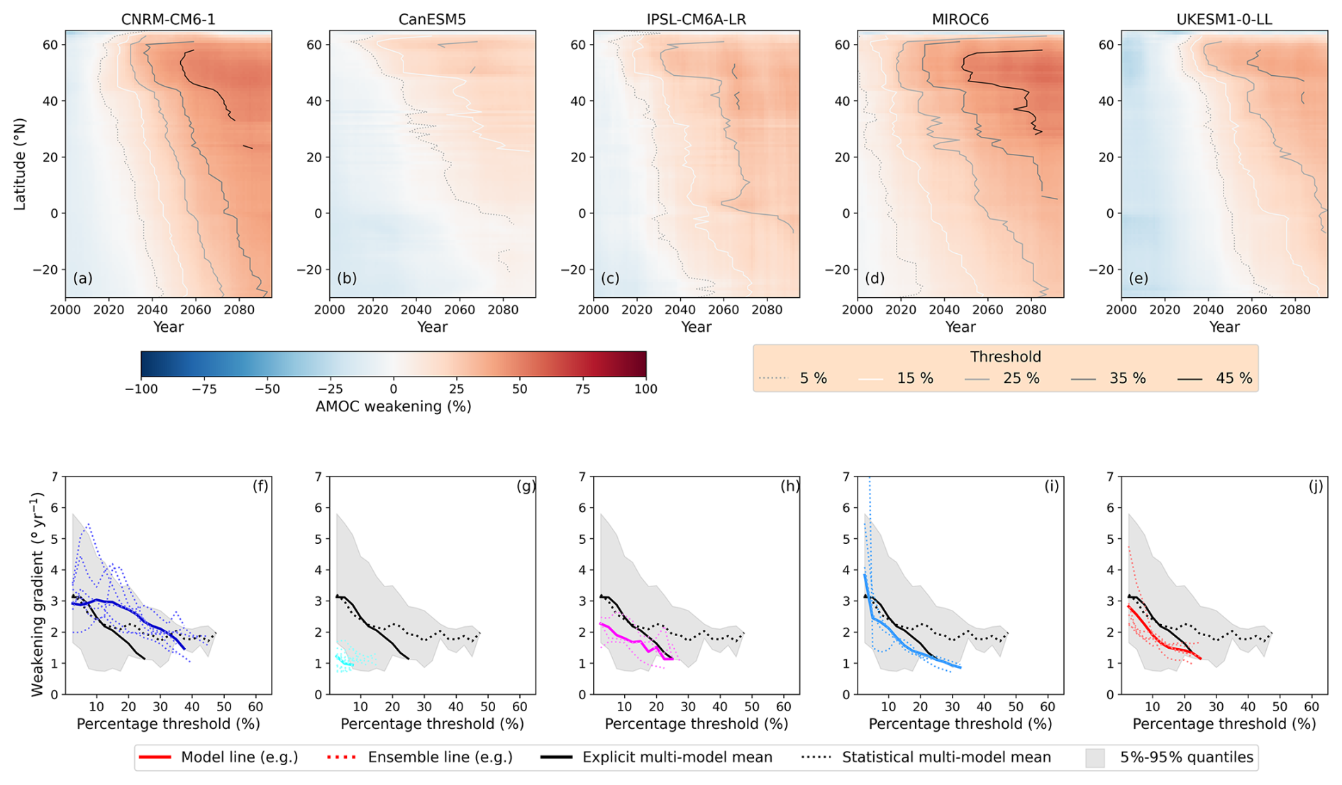
Figure 11 shows the same models as in Fig. 9 but under ssp126 forcing. All models, with the exception of CNRM-CM6-1, show fewer and/or less steep (e.g. slower) threshold lines in the ssp126 experiment (Fig. 11a–e). This is confirmed when looking at the weakening gradients (Fig. 11f–j), where all except CNRM-CM6-1 show a reduction in gradient with increased threshold similar to the EMMM, although for CanESM5 it is hard to make a definitive statement as the ensemble mean weakening gradients do not reach the 10 % threshold. Unlike its ssp585 behaviour, the weakening gradients of CNRM-CM6-1 maintain at ∼ 3° yr⁻¹ until the 15 % threshold before reducing. An interpretation of this is that for CNRM-CM6-1, the initial onset of AMOC weakening is largely resultant from the historical forcing and associated feedbacks and only after the cumulative effects of the ssp126 forcing has occurred does the weakening gradient start to change. Linking this Sect. 3.2, the SMMM weakening gradients at high percentage threshold of ssp126 are skewed by the behaviours of CNRM-CM6-1 and MRI-ESM2-0 while the EMMM weakening gradient is more consistent with most models (see Appendix D, Fig. D4).

As is seen with CNRM-CM6-1 (Fig. 11b), it is possible for weakening signals to propagate under ssp126 forcing similarly or faster to those under ssp585 forcing (Fig. 9b). Understanding model differences in response to different forcing scenarios will give a clearer understanding of how AMOC weakening propagates throughout the Atlantic.

4 Discussion

This study explored AMOC weakening as a function of time and latitude in four CMIP6 future scenarios. The analysis focused on threshold lines and weakening gradients, which show a north-to-south propagation of AMOC weakening initiating in the subpolar North Atlantic (Fig. 3). Variation in the speed and extent of southward propagation are dependent on future forcing scenario and the threshold of weakening (Figs. 6 and 8). Reduction in weakening gradient is suggested to be both scenario and model dependent; for the MMM in the high emissions scenarios (ssp585, ssp370) the weakening gradient reduces then plateaus at higher thresholds (> 20 %) while for low emissions scenarios (ssp245, ssp126) it reduces continuously. An interpretation of these results is that there could be two mechanisms at play, a low threshold/low forcing declining signal in the weakening gradient seen in ssp245 and ssp126 and a high threshold/high forcing constant weakening gradient which the AMOC transitions to. Additionally, weakening in the lower emissions scenarios is more locally constrained to the North Atlantic. It is unclear if the reduction of the weakening gradient, and by inference the propagation speed, is the cause or the result of this local constraint.

There are broad similarities with weakening gradients and the magnitude of AMOC weakening in depth-space and density-space south of 40° N, which is expected given the similarities of the streamfunctions at these latitudes (Kwon and Frankignoul, 2014). Crucially, north of 40° N the density-space streamfunction reveals a higher latitude of origin of the weakening signal for each given threshold and, as seen in Fig. 3, weakening occurs earlier and at higher latitude in density-space than depth-space. While the time difference between 45 and 26° N is comparable for depth-space and density-space (8 and 11 years, respectively, for 25 % weakening in ssp585), when considering measurements at latitudes corresponding to OSNAP and RAPID, density-space shows weakening at OSNAP precedes weakening at RAPID by ∼ 17 years, while ∼ 5 years in depth-space (for 25 % weakening). This substantial difference is due to the latitude of weakening onset being further south in depth-space. As such, when considering latitudinal connectivity of AMOC weakening, the use of density-space is more informative than depth-space (in agreement with Zhang, 2010) showing signals of weakening earlier and suggests it has greater potential for developing early warning signals.

We suggest that the mechanism of weakening gradients is an advective process. A representative weakening gradient value of 2° yr⁻¹ (i.e. reducing from ∼ 3 to ∼ 1.5° yr⁻¹) approximates to a propagation speed of 0.6 cm s⁻¹. Density anomalies advected by internal Kelvin waves with wave speed $c=\sqrt{g_{r}h}=\sim$ 1 m s⁻¹ propagate several orders of magnitude too large to explain the observed weakening gradients (Zhang, 2010; Marshall and Johnson, 2013). Instead, we propose that the negative density anomaly at the western boundary that results from cessation of deep mixing in the convective source areas of deep water formation is advected by the mean flow composing of the DWBC and interior pathways. The negative density anomaly reduces the west-east pressure gradient that drives the southward deep branch of the AMOC (Buckley et al., 2012; Marotzke and Klinger, 2000). Because the mean flow, in turn, is reduced when the west-east pressure gradient reduces, the weakening gradient of the AMOC reduces as the AMOC itself weakens. The majority of models used in this study (67 %, including three of the five models with multiple ensemble members), reduce as the AMOC weakens in support of this argument. While not conclusive evidence, the linear relationship between AMOC weakening and weakening gradients for CNRM-CM6-1 and UKESM1-0-LL suggests that advection may be the main mechanism for propagates mean state AMOC weakening.

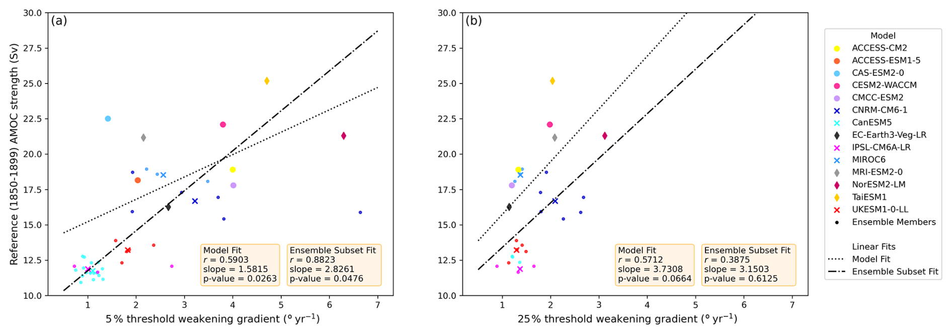
Figure 12 Historical reference (1850–1899) AMOC strength against (a) 5 % and (b) 25 % threshold weakening gradients in density-space. Linear trends are calculated using the full model set (Model Fit) as well as the subset of models that have multiple ensemble members and were the focus of Sect. 3.3 (Ensemble Subset Fit). Note, the absence of EC-Earth3 is due to it lacking weakening gradients at these thresholds.

We find there is a statistically significant positive trend (p < 0.05) between the historical reference AMOC strength and low threshold (≤ 10 %) weakening gradients (shown for the 5 % threshold in Fig. 12a). The trends are shown for both the full model set (see Table 1) with p=0.026 and the subset of models with multiple ensemble members (Table 2) with p=0.048. For these calculations, models with multiple ensemble members are represented by their ensemble mean. The relationship breaks down at higher thresholds (shown for 25 % threshold, Fig. 12b). A positive relationship between reference AMOC strength and the low threshold weakening gradients would support the advective mechanism of weakening gradients, i.e. the initial strength of the AMOC determines the initial speed of propagation of AMOC weakening. However, we treat the results shown in Fig. 12 cautiously, due to inherent uncertainties in the weakening gradient method explored in Sect. 3.3, such as for models with single ensemble members and models where weakening does not span the full basin (IPSl-CM6A-LR).

Given all the models in this study are non-eddying, with a horizontal resolution of ∼ 1°, the real world applicability of these results may be limited and the weakening gradients may be faster than shown here due to better resolved eddy processes (Hodson and Sutton, 2012; Weijer et al., 2012) and stronger boundary currents. Additionally, while we propose the mechanism of propagation to be advective, it has been noted that low resolution models do not adequately represent wave-mediated adjustment. We hypothesise that weakening in high resolution models will still be transported advectively but it may be that wave mechanisms are more involved and result in faster propagation timescales. A recent pre-print article suggests connectivity of decadal variability in the Atlantic is greater at higher resolution (Rapanague et al., 2026). The study uses pre-industrial climate forcing and it would be interesting to see similar analysis holds under future climate forcing. Increasing the number of higher resolution models running the future scenario experiments and outputting the necessary variables to analyse the AMOC streamfunction would be essential to address the effect of resolution on propagation speed. Whether the differences seen in weakening gradient behaviours indicate different mechanisms of AMOC weakening propagation in the ensemble of 1° resolution CMIP6 models requires further work.

In the inter-model comparison, it was shown that for individual models AMOC weakening often has its onset in the SPG and it does not always immediately translate to AMOC weakening further south (Fig. 9). The strength of the SPG has been shown to increase in some models even as the AMOC weakens (see Fig. 8 in Dong et al., 2025) and the relationship between the SPG strength and the AMOC is an active area of research. Changes to the mixed layer depth (MLD) at sites of deep convection have not been considered in this study but are vitally important for understanding the changes to the AMOC (e.g. Drijfhout et al., 2025).

The rate of AMOC weakening in ssp370 is slower than the other scenarios (Figs. 5 and 7), contrary to the findings of Weijer et al. (2020). It's possible this disagreement could be related to the specific models chosen to study or the differences in methodology. Menary et al. (2020) showed aerosol forcing in CMIP6 strengthens the AMOC and we propose the increased aerosol content in ssp370 is what slows the weakening. The response to aerosols may be overstated in CMIP6 compared to reality (Robson et al., 2022) so our results may be more pronounced than observations would show. Despite this oversensitivity, we argue ssp370 is a valuable experiment when considering AMOC changes in the first half of the 21st century due to the slower response of weakening than seen in the other future climate scenarios.

Here we discuss the role of internal variability and weakening on interannual timescales, which are not included in the main results due to the limited number of ensemble members used. The impact of interannual variability is addressed by applying decadal smoothing and multi-decadal variability has been partly resolved by the use of multiple ensemble members in Sect. 3.3. However, 10 of the 15 models in this paper have only one ensemble member available and others only had very few (e.g. IPSL-CM6A-LR only had three). For these models, the threshold lines can become increasingly noisy especially as the signal of internal variability spans the basin faster than the signal of weakening. This is a limitation of the first exceedance framework used to identify the threshold lines. Appendix F contains timeseries of relative AMOC strength at 51° N (Fig. F1) and 26° N (Fig. F2), to reveal the extent of internal multi-decadal variability. Models with multiple ensemble members were emphasized in Sect. 3.3 to increase confidence in capturing the AMOC mean state change with the threshold lines and not signals from internal variability. Another limitation of the threshold method is the requirement for a reference AMOC to compare AMOC weakening against. The chosen reference period cannot be too close to the start of the time period of interest (2015–2100), otherwise one might not capture the true onset of a weakening signal and threshold line, and weakening gradients represent a deviation from the reference rather than propagation. This was found to be the case when using a reference of 1995–2014 (not shown). The reference period chosen was 1850–1899, however this has its own uncertainties associated with a sparsity of measurements from this time (Robson et al., 2022). However, these two issues of internal variability and uncertainty in the historical reference are by no means unique to this study.

5 Conclusions

Using future climate projections from CMIP6 ScenarioMIP we have shown AMOC weakening propagates southward from the high latitude North Atlantic to the southern boundary of the Atlantic (∼ 30° S). The southward propagation of AMOC weakening is measured by looking at the percentage AMOC decline relative to a historical reference AMOC strength. The origin of weakening density-space representation occurs at a higher latitudes than depth-space (45–51° N in depth-space and 51–61° N in density-space, Fig. 3). The behaviour of weakening propagation is dependent on the future climate change scenario. As the AMOC weakens, the propagation speed reduces, with the MMM weakening gradient under ssp585 forcing reducing from ∼ 3.0 to ∼ 1.4° yr⁻¹ (Fig. 4). The behaviour of weakening propagation is dependent on the future climate forcing scenario (Fig. 8). Furthermore, the behaviour of weakening gradients to AMOC weakening is highly model dependent and, in the case of CNRM-CM6-1, also dependent on the ensemble member (Fig. 11). Improving the understanding of latitudinal connectivity of AMOC weakening in the subpolar North Atlantic and southward could be critical to reducing uncertainties in our climate projections and aid the development of early warning signals of potential AMOC weakening or collapse (Jackson and Wood, 2020). Understanding the driving mechanism for southward propagation of AMOC weakening and what determines the different speeds of the weakening gradients between models could also provide insight into the CMIP6 model spread. Better understanding of model spread should lead to improved models and improved confidence in predictions of AMOC weakening in the 21st century.

Appendix A: Depth-space streamfunctions: online vs offline

The depth-space AMOC streamfunction is computed by integrating meridional velocities as described in Hirschi and Marotzke (2007) and in this study (Sect. 2). This study primarily uses streamfunctions calculated from meridional velocity data available in the CMIP archive used (referred to as “offline”). The AMOC streamfunctions are often, but not always, provided by the modelling centres (referred to as “online”). The exact details of how the AMOC is computed offline can lead to differences with the online streamfunction. Meridional velocity in the CMIP archive is provided in two different variables “vo”, the meridional velocity without the bolus velocity in m s⁻¹ and “vmo” the meridional mass transport including the bolus velocity in kg s⁻¹ which requires using a reference density (1026 kg m⁻³) to convert to a velocity. The exact definition of the Atlantic basin can differ and whether the depth or section average velocity has been removed before computing the streamfunction. Here, we compare differences in computing the AMOC streamfunction both online and offline.

We show this difference for models that have online streamfunctions readily available (Fig. A1, column 1), as well as both vmo (Fig. A1, column 2) and vo (Fig. A1, column 4) variables available too. We refer to both vmo and vo as offline streamfunctions. The differences in the available streamfunction and the vmo and vo streamfunctions are shown in Fig. A1, column 3 and 5, respectively. Comparisons show that the offline AMOC streamfunction computed using the mass transport reproduces the online streamfunction closely (Fig. A1). This difference is likely due to the inclusion of the bolus transport in vmo data that is not present in the vo data. The magnitude of difference for the offline vmo streamfunctions is small (≪ 0.1 Sv) for all models except CanESM5 and ACCESS-ESM1-5, while the magnitude of difference in the vo streamfunctions is on the order 1 Sv, with some larger disagreements, for example at the surface near 40° N. This shows that the vmo streamfunction captures the behaviour of the online streamfunction more completely than the vo streamfunction does. The calculated streamfunctions excluded the Mediterranean and including the Mediterranean removes the ∼ 1 Sv difference in the CanESM5 vmo calculations (not shown).

ACCESS-ESM1-5 is the only model where it is not obvious whether vmo or vo reproduces a more accurate streamfunction. The vmo streamfunction contains an error at 4° S. We note ACCESS-ESM1-5 is a sigma-level model that has been interpolated onto a regular z-level grid. Investigating the vmo and vo output, we found the bathymetry at the same z-level between these two outputs was subtly different and suggest the vertical grid for these two outputs are not properly aligned. Shifting the vmo streamfunction up by one vertical level reduces most of the streamfunction differences to less than 1 Sv (not shown). We speculate the alignment issue may be the cause of the error at 4° S.

Furthermore, there is very little difference between the maximum strength and latitude of the maximum streamfunction (Fig. A2), with the exception of ACCESS-ESM1-5, all models sit on the y=x line between the online and offline vmo depth-space streamfunctions and for practical purposes we can treat these streamfunctions as identical. This is contrasted with the comparison between the online and offline vo depth-space streamfunctions (Fig. A3), where vo AMOC strength is consistently ∼ 1 Sv lower than the online product (see also Menary et al., 2020 Fig. S1) and onset latitudes show wide deviation from the y=x line. We therefore suggest when comparing online and offline streamfunctions, the use of vmo to calculate volume transport is better than the use of vo. For this study we prioritise the use of offline streamfunctions and as the density-space streamfunctions are calculated offline using vo, we choose to the use the offline vo streamfunctions for consistency.

Finally, we compare weakening Hovmöller using the vo streamfunctions to a weakening Hovmöller using a hybrid group of online and vmo streamfunctions (Fig. A4). Structurally, these threshold lines are very similar but the vo threshold lines lead the online/vmo by approximately 1–3 years at the latitudes of onset. This is likely due to the vo streamfunctions being ∼ 1 Sv weaker than the online streamfunctions (Fig. A1), attributed to the bolus velocity. As a result, the same absolute change in AMOC strength (e.g. 3 Sv) will result in a larger percentage change for vo than vmo and so the percentage threshold appears sooner in the north. South of 30° N, the vo and vmo threshold lines agree, with differences only of order 1 year at most.

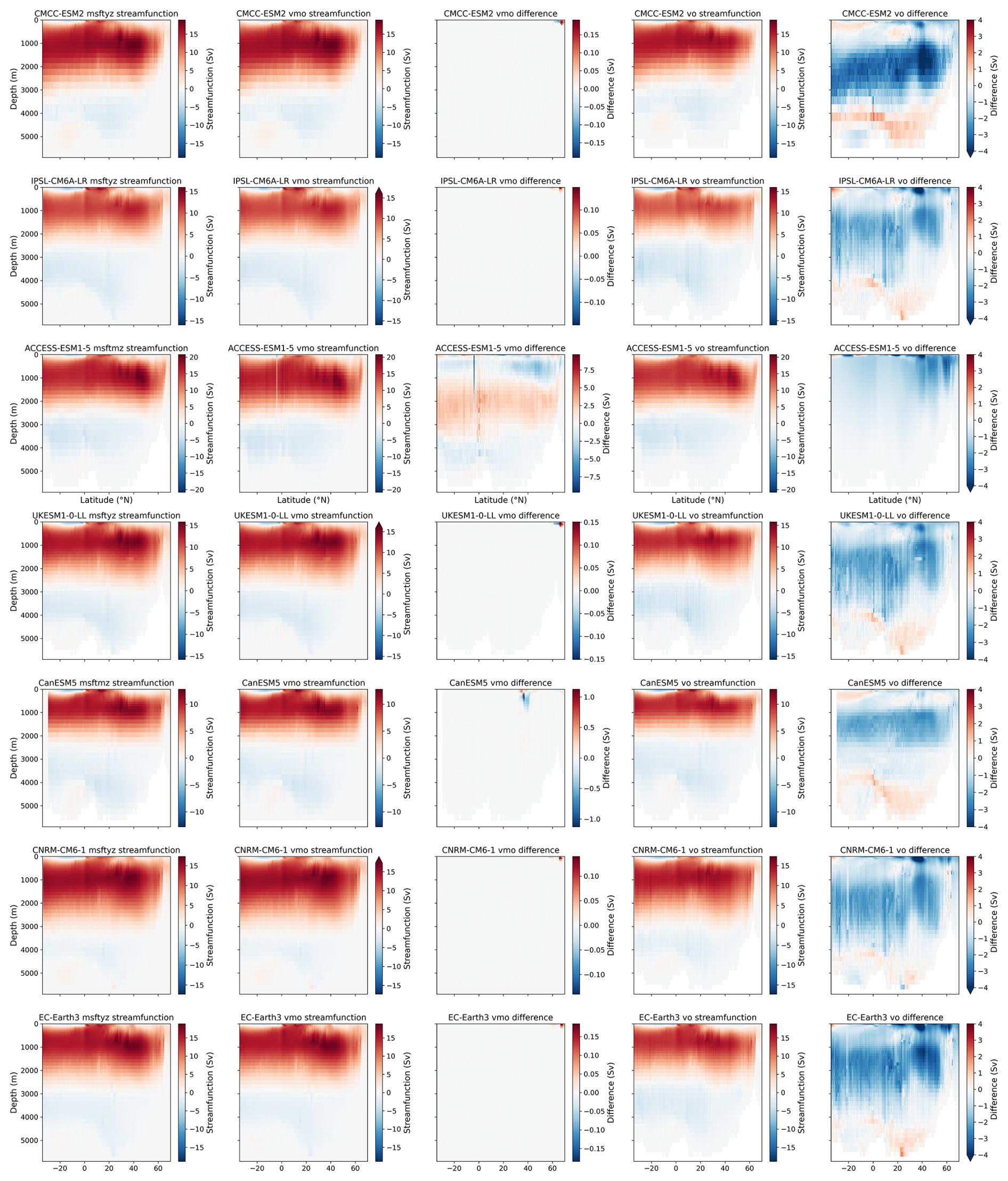
Figure A1 Online depth-space streamfunctions (column 1), offline depth-space streamfunctions calculated with vmo (column 2) and vo (column 4) variables. The difference in streamfunctions, offline subtracted by the online streamfunctions (column 3 and column 5 for vmo and vo, respectively).

For the vo group, we use the same streamfunctions as used in the main body of text (see Table 1). For the online/vmo group, ACCESS-CM2, ACCESS-ESM1-5, CAS-ESM2-0, CESM2-WACCM, MIROC6, MRI-ESM2-0, NoRESM2-LM and UKESM1-0-LL use online streamfunctions and CanESM5, CMCC-ESM2, CNRM-CM6-1, EC-Earth3, EC-Earth3-Veg-LR and IPSL-CM6A-LR use vmo streamfunctions. TaiESM1 uses the vo streamfunction as it does not have vmo available.

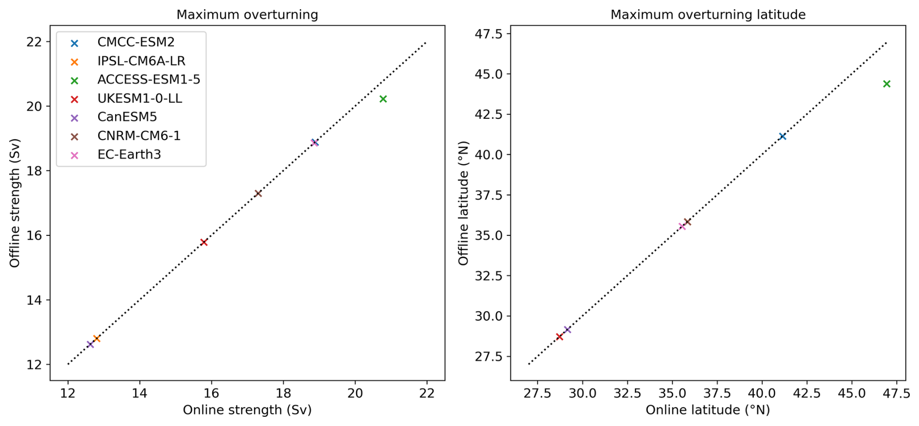
Figure A2 Left: AMOC strength maxima for the online and vmo streamfunctions. Right: Latitude of the maximum overturning for the online and vmo streamfunctions. Taken over the historical period (1850–1899).

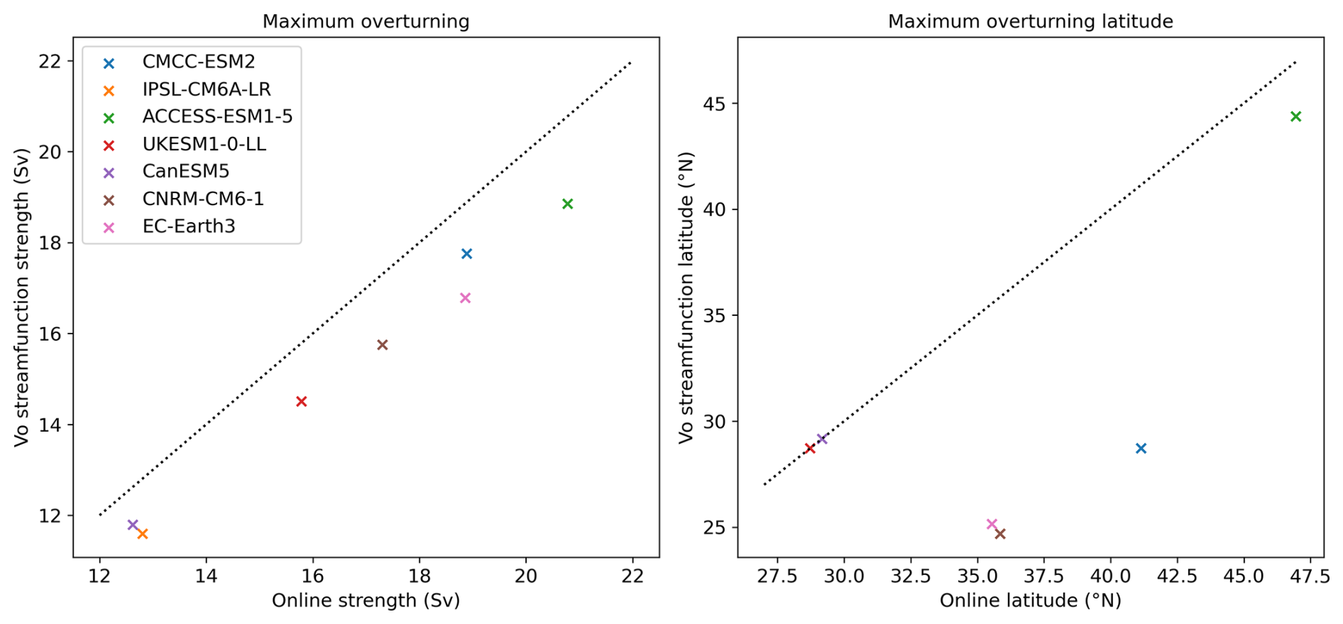
Figure A3 Left: AMOC strength maxima for the online and vo streamfunctions. Right: Latitude of the maximum overturning for the online and vo streamfunctions. Taken over the historical period (1850–1899).

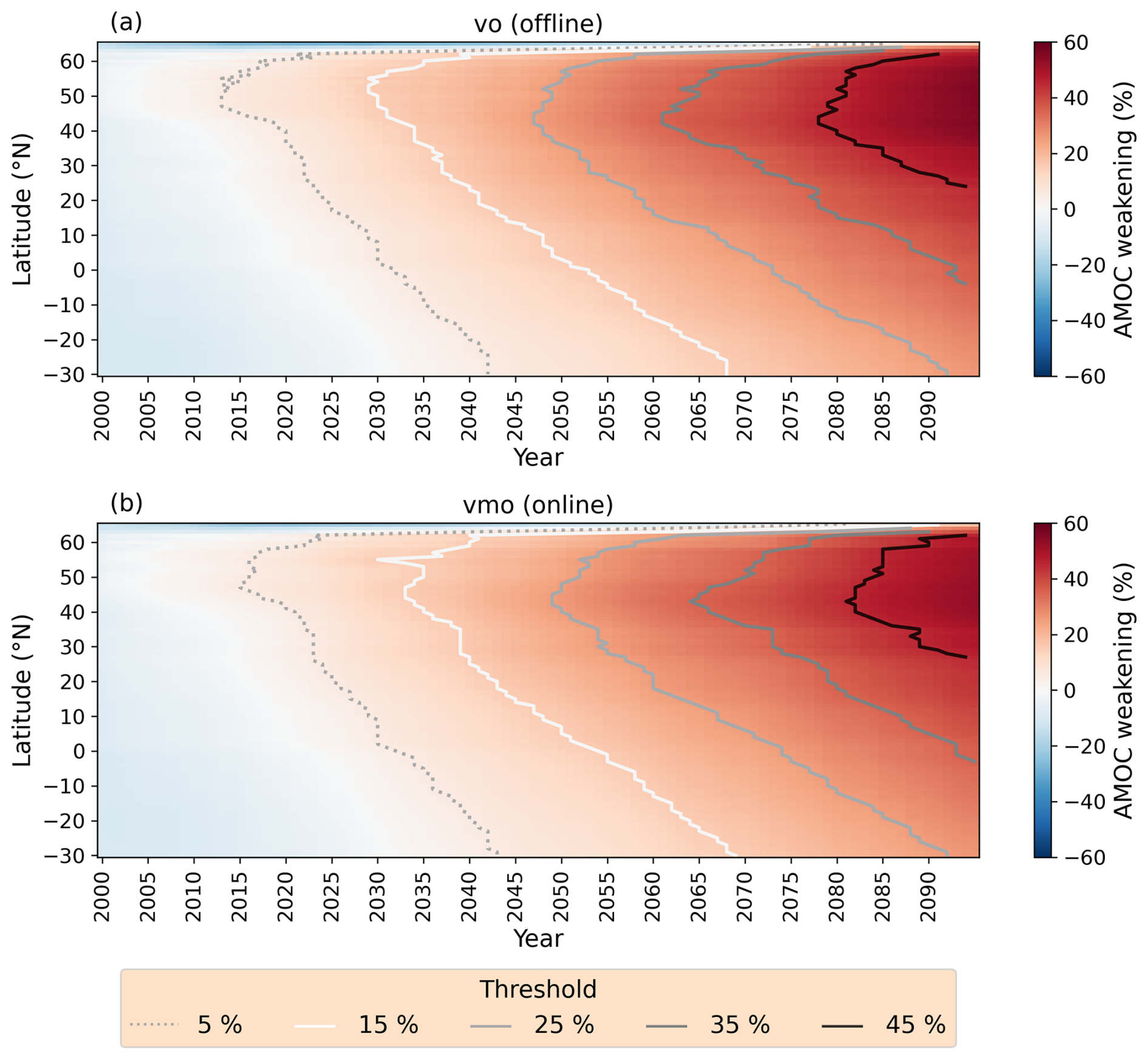
Figure A4 Hovmoller weakening diagrams for the ssp585 scenario, for (a) the offline calculated vo streamfunction and (b) the hybrid online/vmo dataset. The 5 %, 15 %, 25 %, 35 % and 45 % threshold lines are shown.

Appendix B: Density-space streamfunctions: online vs offline

For modelling centres with available density-space AMOC streamfunctions, we compare the provided density-space streamfunctions, which we refer to as online (Fig. B1, column 1), to our calculated density streamfunctions as described in the methods section (Fig. B1, column 2), which we refer to as offline. The models used for this comparison are ACCESS-CM2, ACCESS-ESM1-5, MRI-ESM2-0 and NorESM2-LM. The differences of these streamfunctions are shown in Fig. B1, column 3. The difference in streamfunction is large (> 3 Sv) for all models near the boundary between subtropical and subpolar gyre ∼ 40° N. These differences are reminiscent of the differences in the depth-space vo streamfunction as seen in Fig. A1, column 5. This difference is understandable, given that the meridional velocity (vo) does not include the bolus velocity. We also note that these four models are originally sigma-level models. The model output was interpolated onto a z-level grid to produce the variables vo, thetao and so and we have re-interpolated back onto a sigma-level grid. This double interpolation may have introduced errors into our calculation of the density streamfunction.

Figure B2 shows that the maximum overturning strength is lower in the offline streamfunctions than the online ones except for NorESM2-LM, with the maxima differing in the range of 1–3 Sv. With the exception of ACCESS-ESM1-5, the latitude of maximum overturning is the same in the offline and online. The difference in AMOC strength of 1–3 Sv is not insubstantial, however this study focuses primarily on percentage change of AMOC strength and we suggest this is not a substantial issue. Figure B3 shows the weakening Hovmöllers for these four models for the ssp370 experiment. The threshold lines are shown for the online and offline calculations. There is reassuring coherence in the timings and structures of these lines. The most substantial differences are the offset in the 25 % threshold line for ACCESS-ESM5-1 and north of 40° N for MRI-ESM2-0, the online threshold lines are delayed by a few years compared to the offline.

The weakening gradients are also fairly comparable for online and offline (Fig. B4), but we acknowledge they are not identical, especially for ACCESS-ESM5-1 and MRI-ESM2-0. Despite the exact values of the weakening gradients not being identical, the trends in both of these models are the same for online and offline; the trends are a rapid reduction in weakening gradient in ACCESS-ESM5-1 due to internal variability delaying and obscuring southward weakening signals and for MRI-ESM2-0 a steady reduction in weakening gradient as the AMOC weakens.

The weakening gradients, onset latitudes and onset years for the online and offline density streamfunctions are shown in Fig. B5. There is general agreement in the weakening gradients, except for the 5 % threshold for ACCESS-ESM1-5 (Fig. B5, left). There is a generally linear relationship between the onset years of the models, although the offline do skew earlier than the online (Fig. B5, right). The onset latitudes comparisons are more interesting and we shall discuss them model by model. For ACCESS-CM2 and ACCESS-ESM1-5, the onset latitudes are fairly in agreement between online and offline. The 35 % threshold onset latitude for ACCESS-CM2 we believe to be spurious and should be ignored, especially judging from the threshold lines in Fig. B3. MRI-ESM2-0 has a constant ∼ 50° N onset latitude for the offline, while the online varies between 45–65° N. NorESM2-LM shows the opposite trend, where the online onset is fairly constant at ∼ 62° N, while the offline varies between 45–65° N. When ignoring the very high latitudes (north of 60° N), we find the onset latitudes are consistent or within a few degrees of each other, centred around ∼ 50° N, for both MRI-ESM2-0 and NorESM2-LM. These results, in tandem with ACCESS models agreeing, gives us confidence in the offline streamfunction's ability to reasonably reproduce the high latitude weakening onset.

To conclude, we acknowledge there are differences in the offline and online density streamfunction calculations, but argue they are largely constrained to the subpolar latitudes, do not have a substantial impact on the percentage change in AMOC strength (Fig. B3) and thus do not substantially impact calculations of weakening gradients. We therefore have choose combined use of offline and online density streamfunctions.

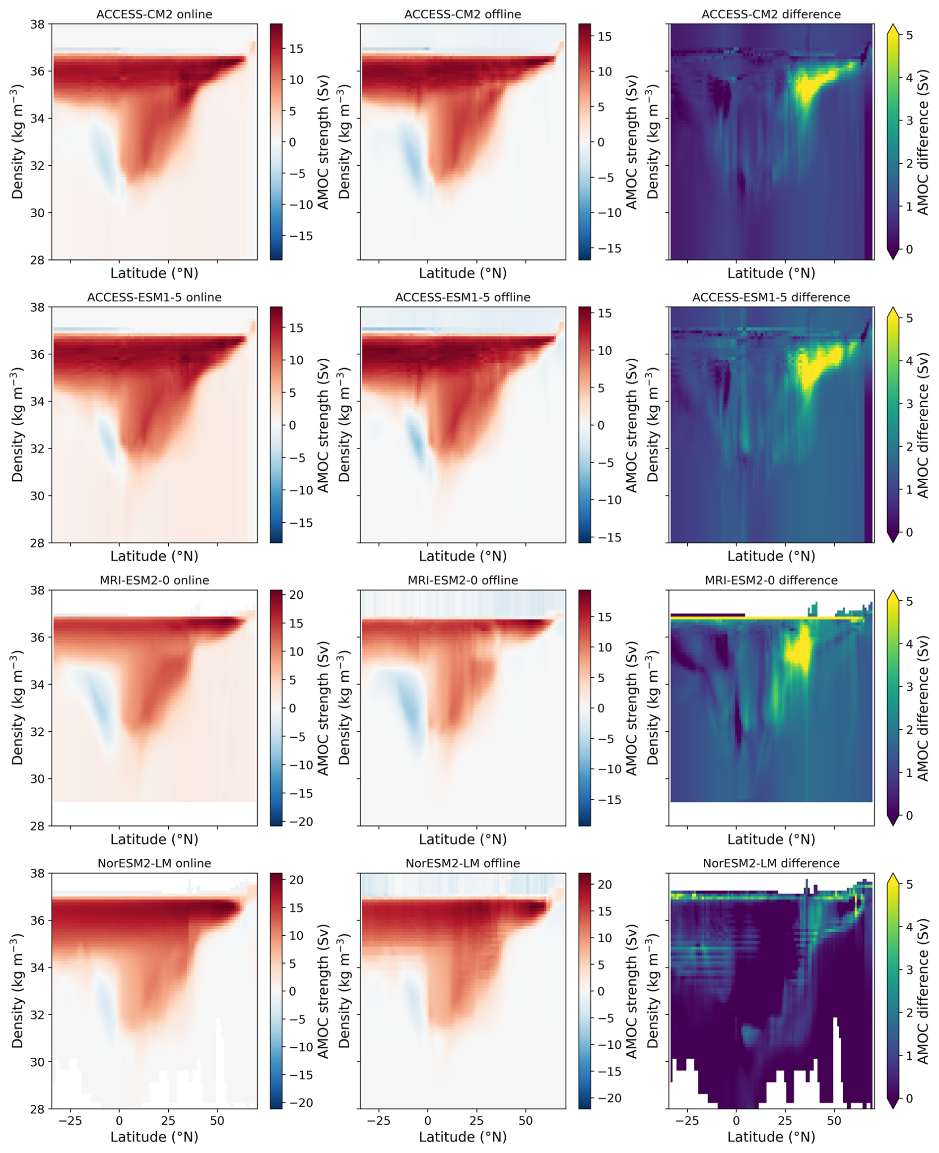
Figure B1 Online density-space streamfunctions (column 1), offline density-space streamfunctions (column 2) and the difference between the two (column 3). Taken over the historical period (1850–1899).

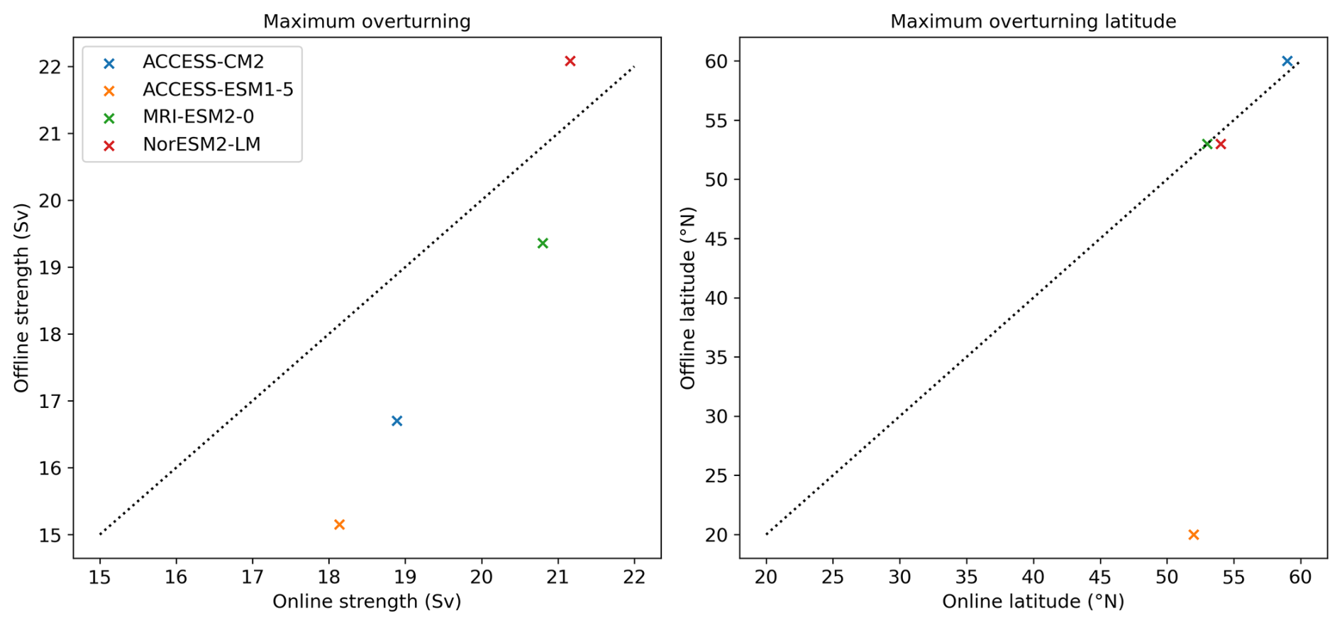
Figure B2 Left: AMOC strength maxima for the online and offline density streamfunctions. Right: Latitude of the maximum overturning for the online and offline density streamfunctions. Taken over the historical period (1850–1899).

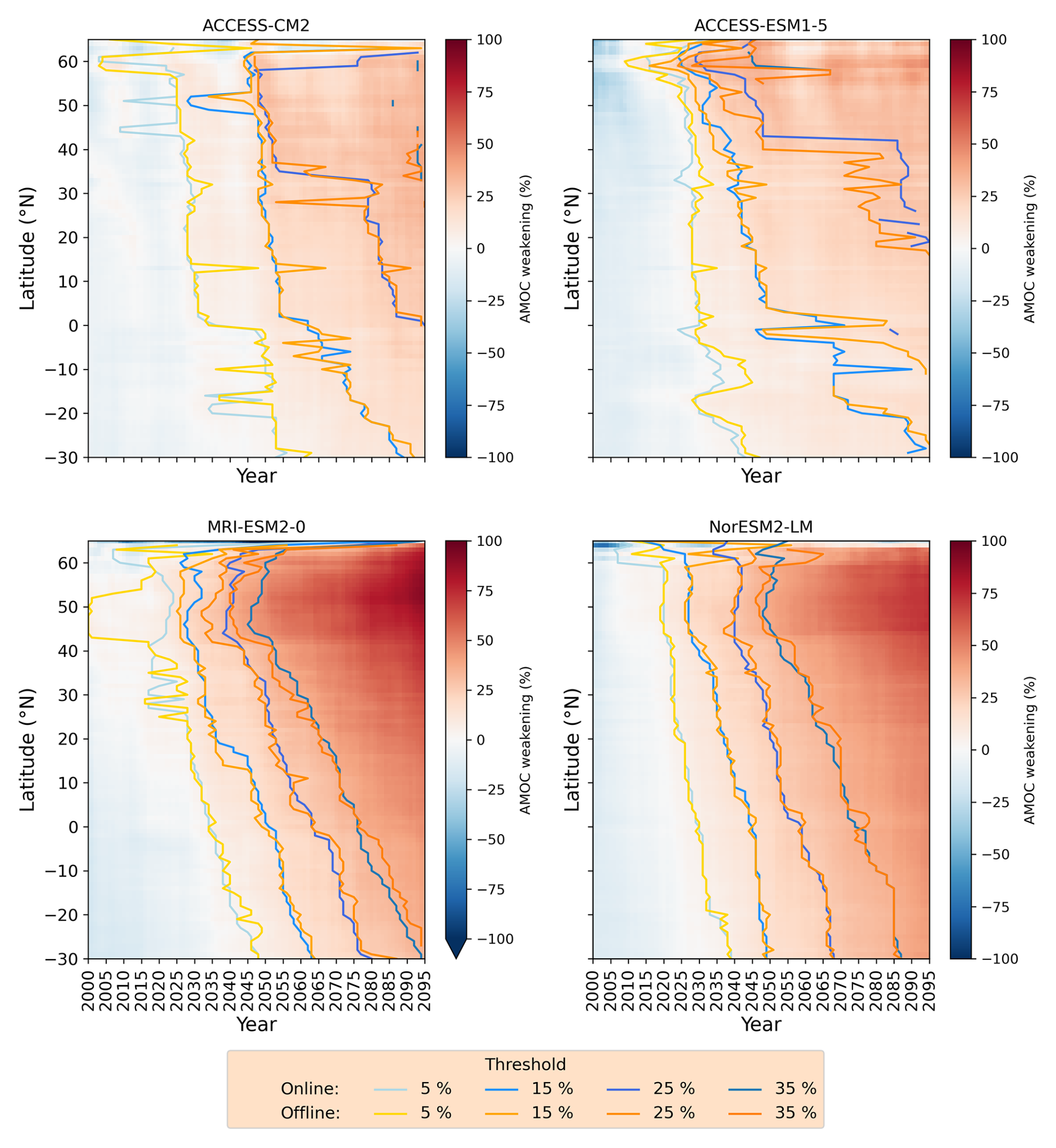
Figure B3 Hovmoller weakening diagrams for the ssp370 scenario, for the offline calculated density-space streamfunction. The 5 %, 15 %, 25 % and 35 % threshold lines are shown as calculated from both the online and offline streamfunctions.

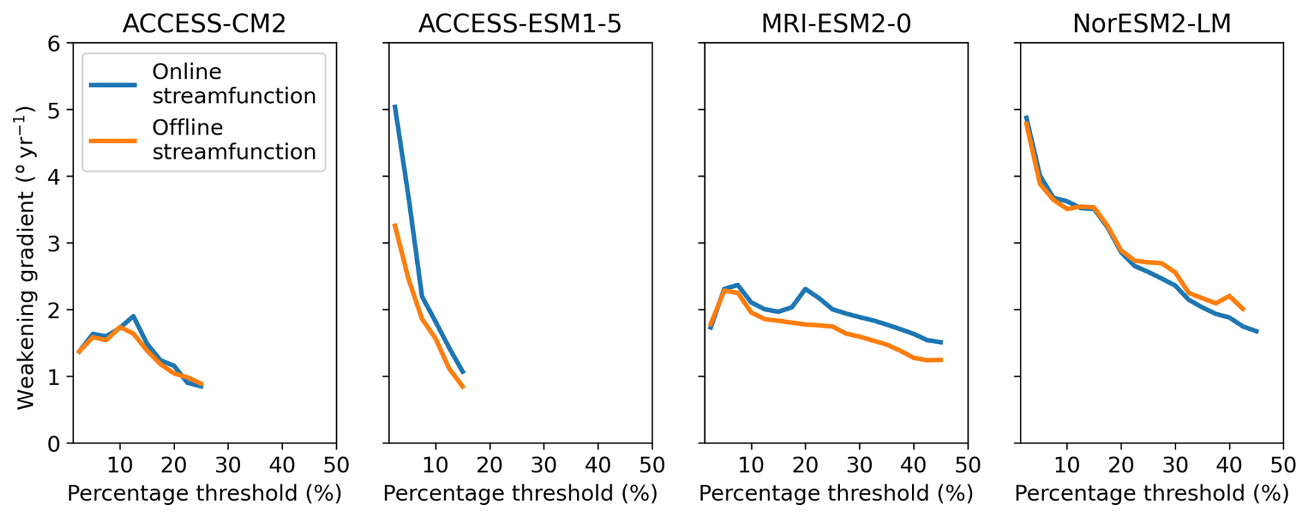
Figure B4 Weakening gradients for the ssp370 scenario, calculated for both the online and offline density-space streamfunctions.

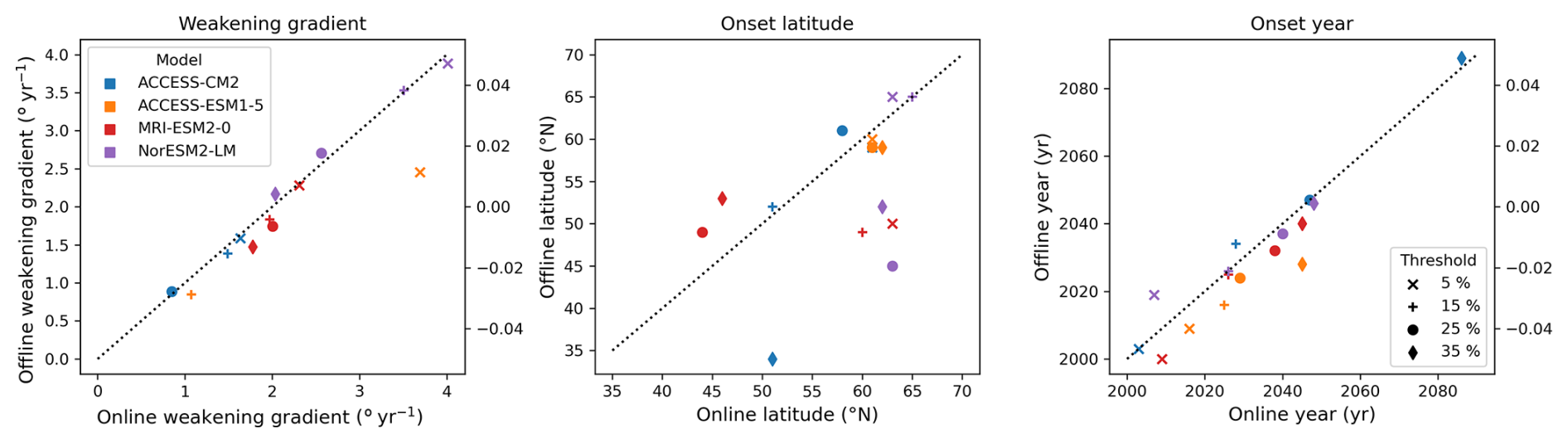
Figure B5 Online and offline threshold weakening gradients (left), online and offline onset latitude of weakening (centre), online and offline onset year of weakening (right). The thresholds included are 5 %, 15 %, 25 % and 35 %. Note ACCESS-ESM1-5 lacks a 25 % and 35 % threshold weakening gradient and ACCESS-CM2 lacks a 35 % threshold weakening gradient.

Appendix C: Statistical Comparisons

We compare the weakening of our model set to the weakening found in Weijer et al. (2020), using the method presented in that paper (Fig. C1). We calculate the percentage strength change between the historical period (1850–2014) as the reference and the final 20 years (2080–2099) of ssp585. We find the mean weakening of this model set is 45 %, which is 6 percentage points higher than the mean weakening of the Weijer et al. (2020) model set.

The p-value and mean r-values for the linear fits of weakening gradients are shown in Figs. C2 and C3, respectively.

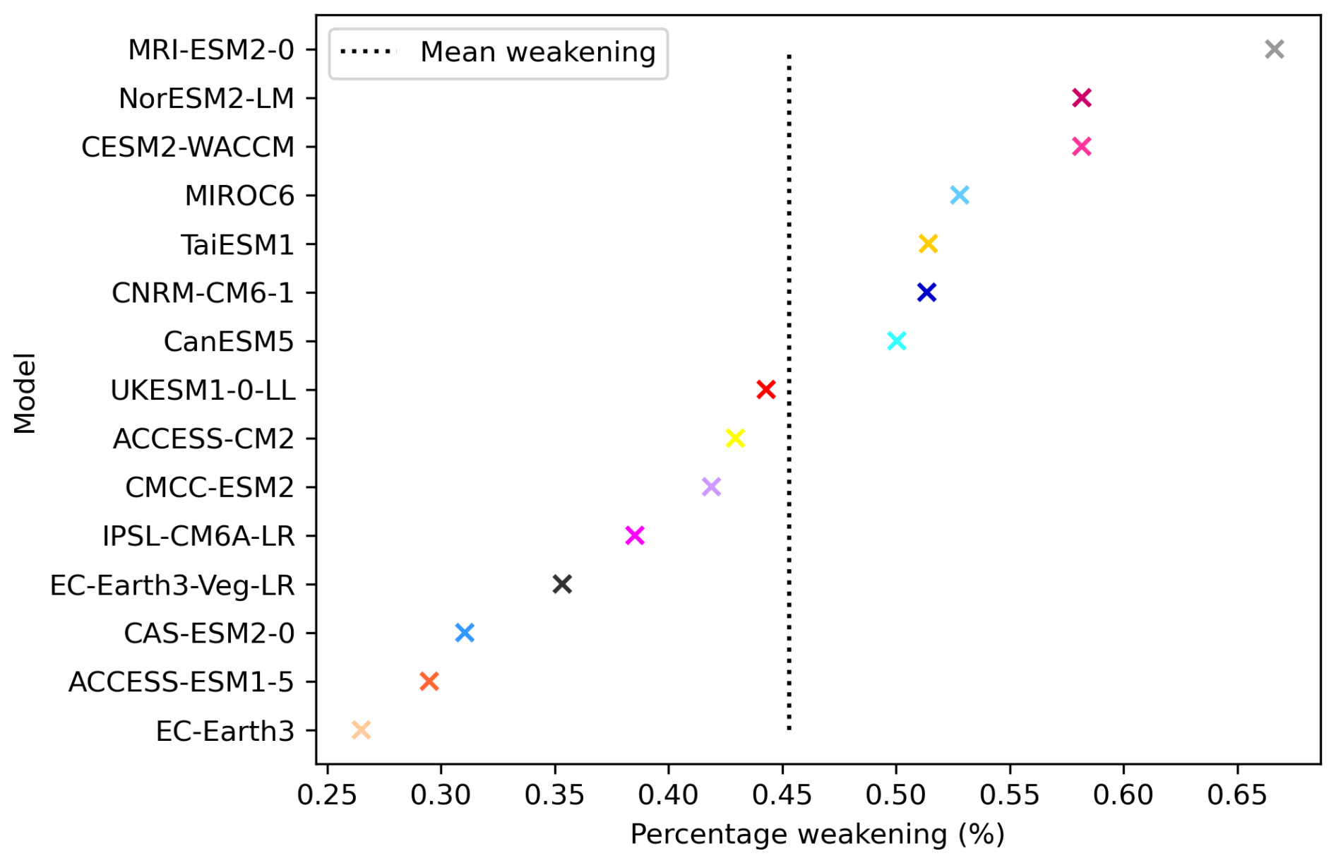
Figure C1 Percentage AMOC weakening using the method from Weijer et al. (2020) for ssp585. The mean weakening of the model set is marked with the dashed line.

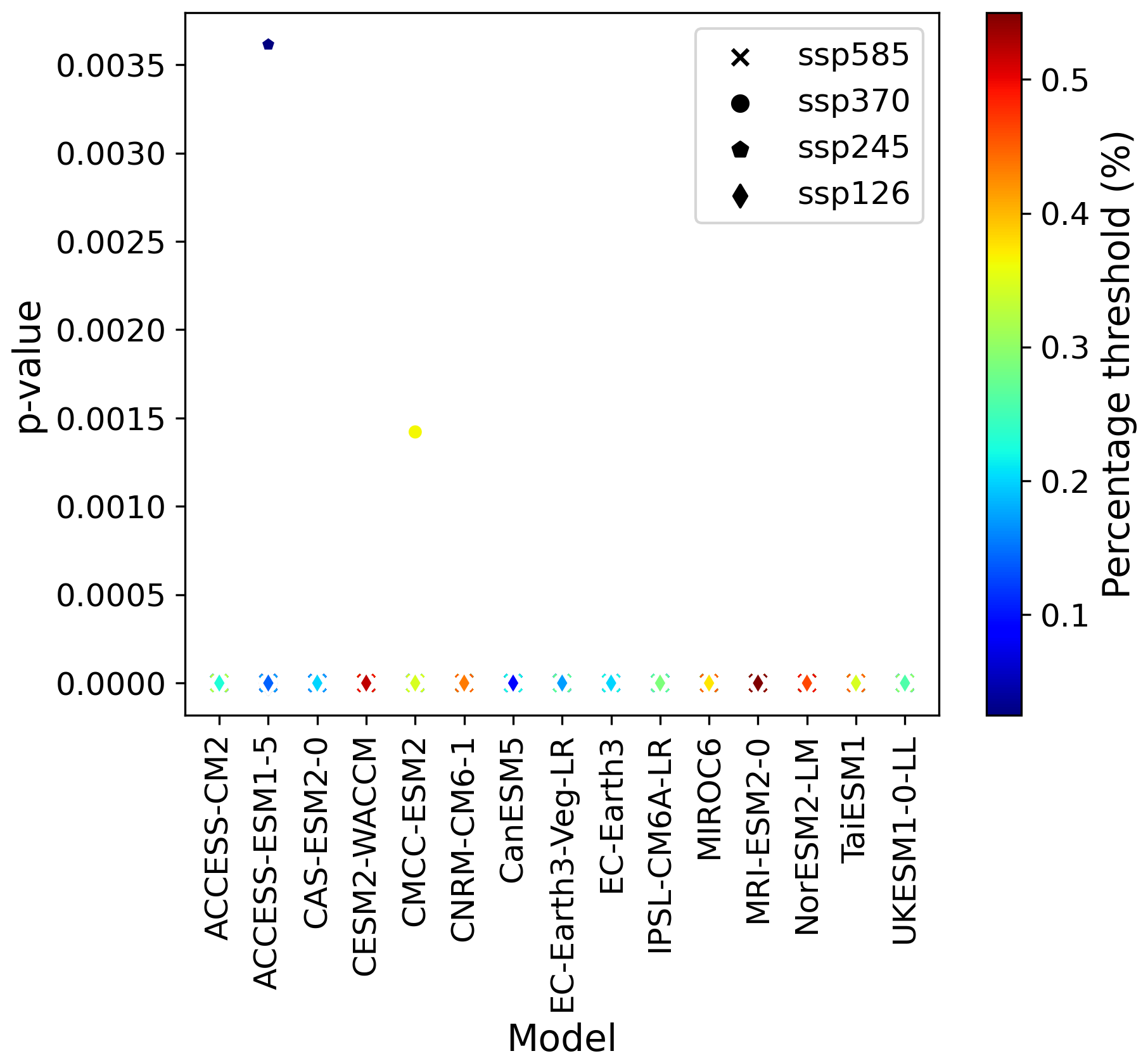
Figure C2 The p-value of the linear fits for the weakening gradients for each scenario for each model.

Figure C3 The mean r-value of the weakening gradients for the four scenarios for each model.

Appendix D: Density Model Set

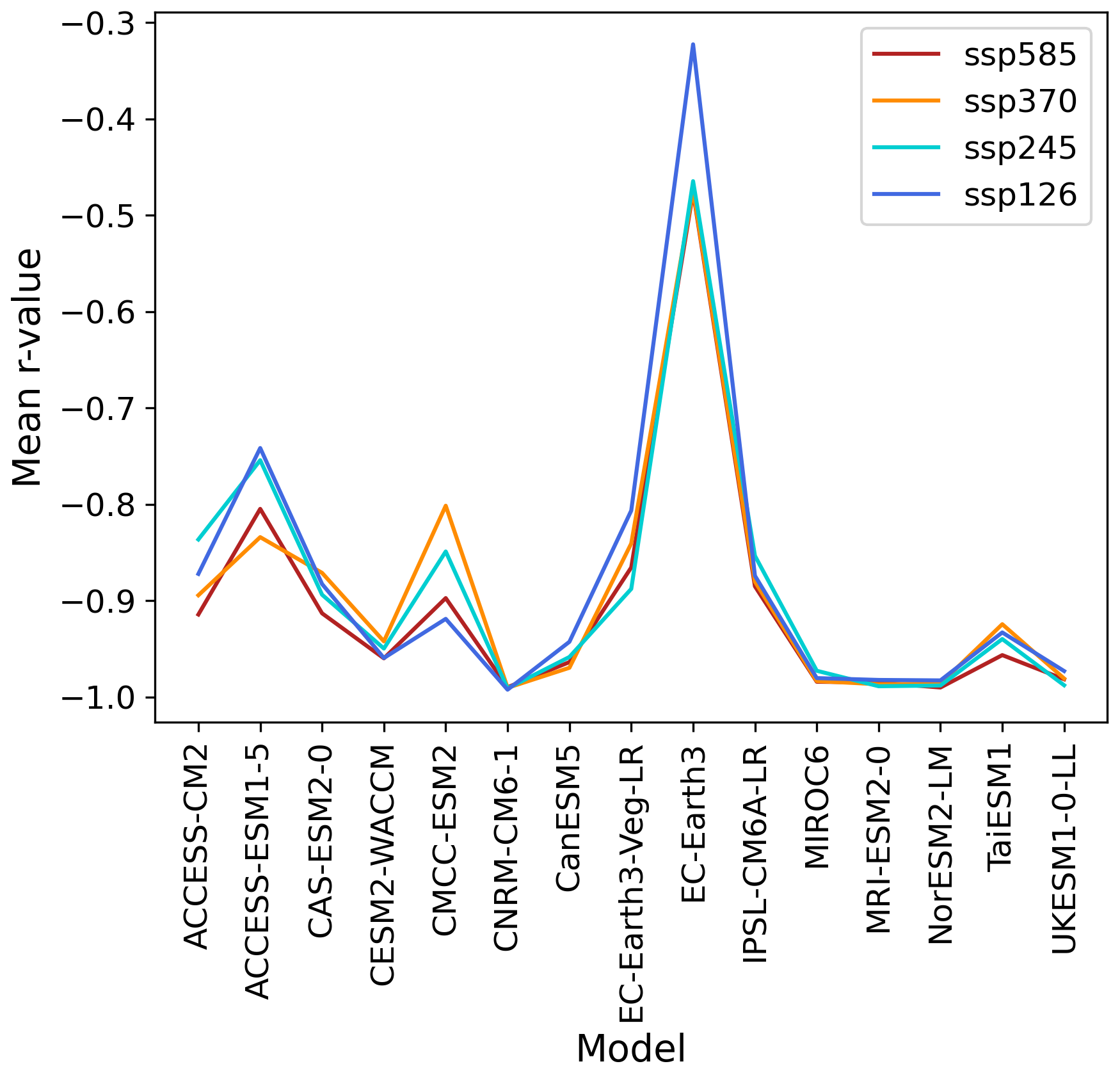
The full model set Hovmöller and weakening gradient plots for density-space.

Figure D1 Weakening Hovmöller in density-space for ssp585.

Figure D2 Weakening Hovmöller in density-space for ssp126.

Figure D3 Weakening gradients in density-space for ssp585.

Figure D4 Weakening gradients in density-space for ssp126.

Figure D5 Weakening Hovmöller for individual ensemble members in density-space for ssp585.

Appendix E: Depth Model Set

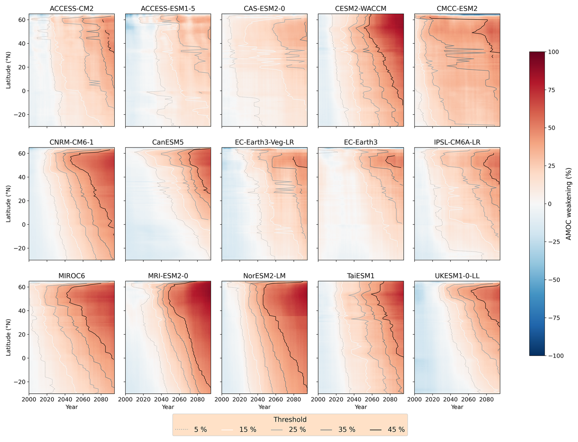
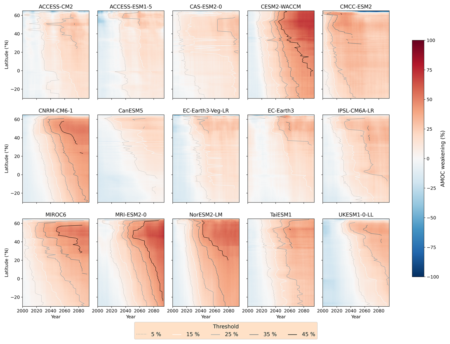
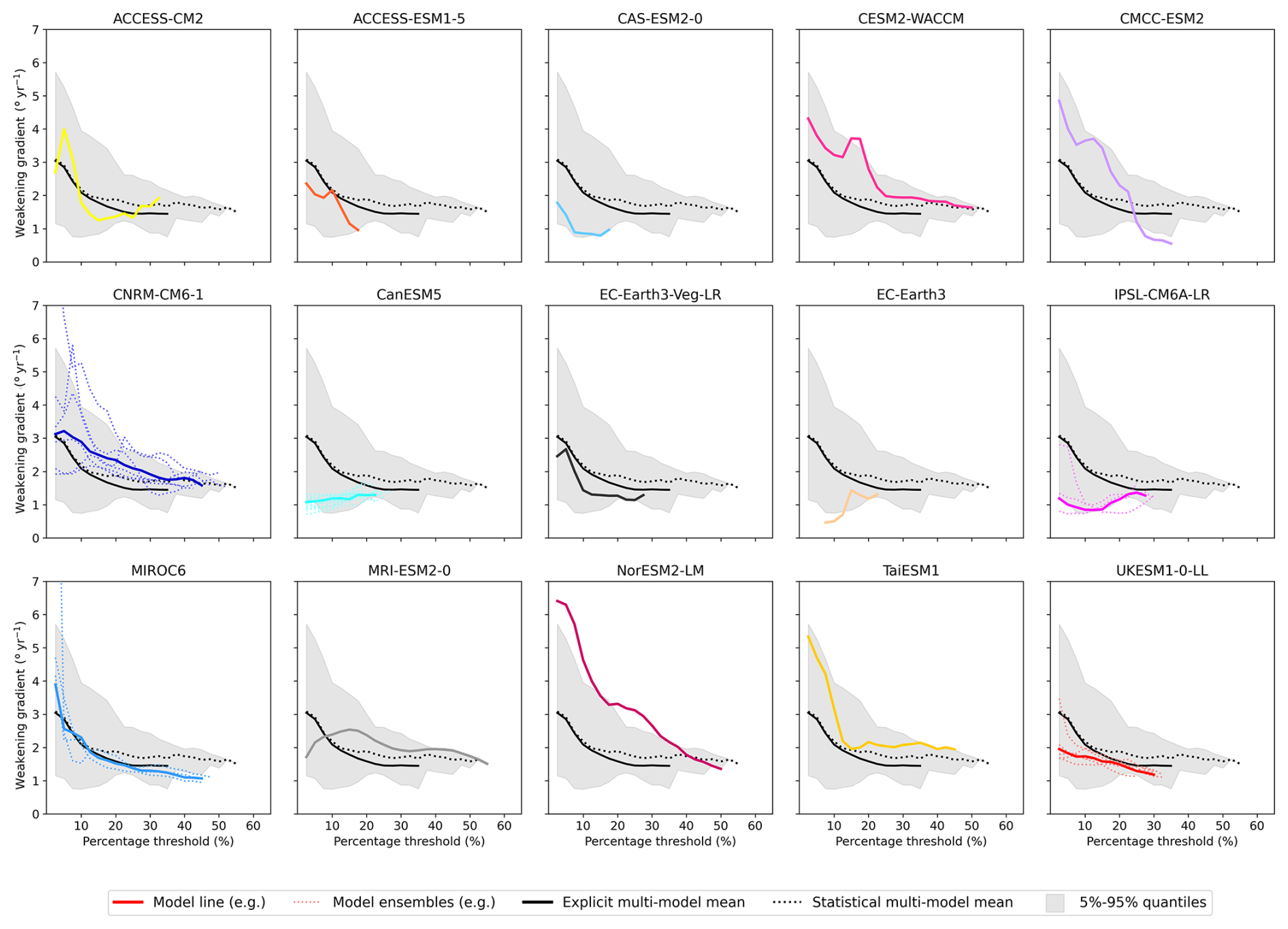
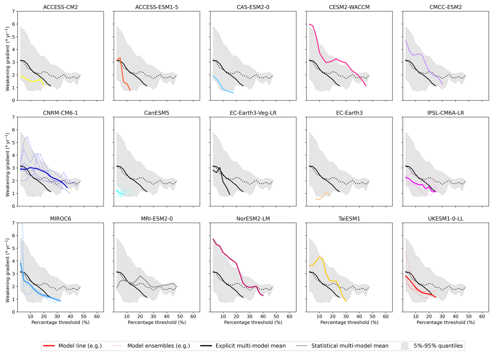
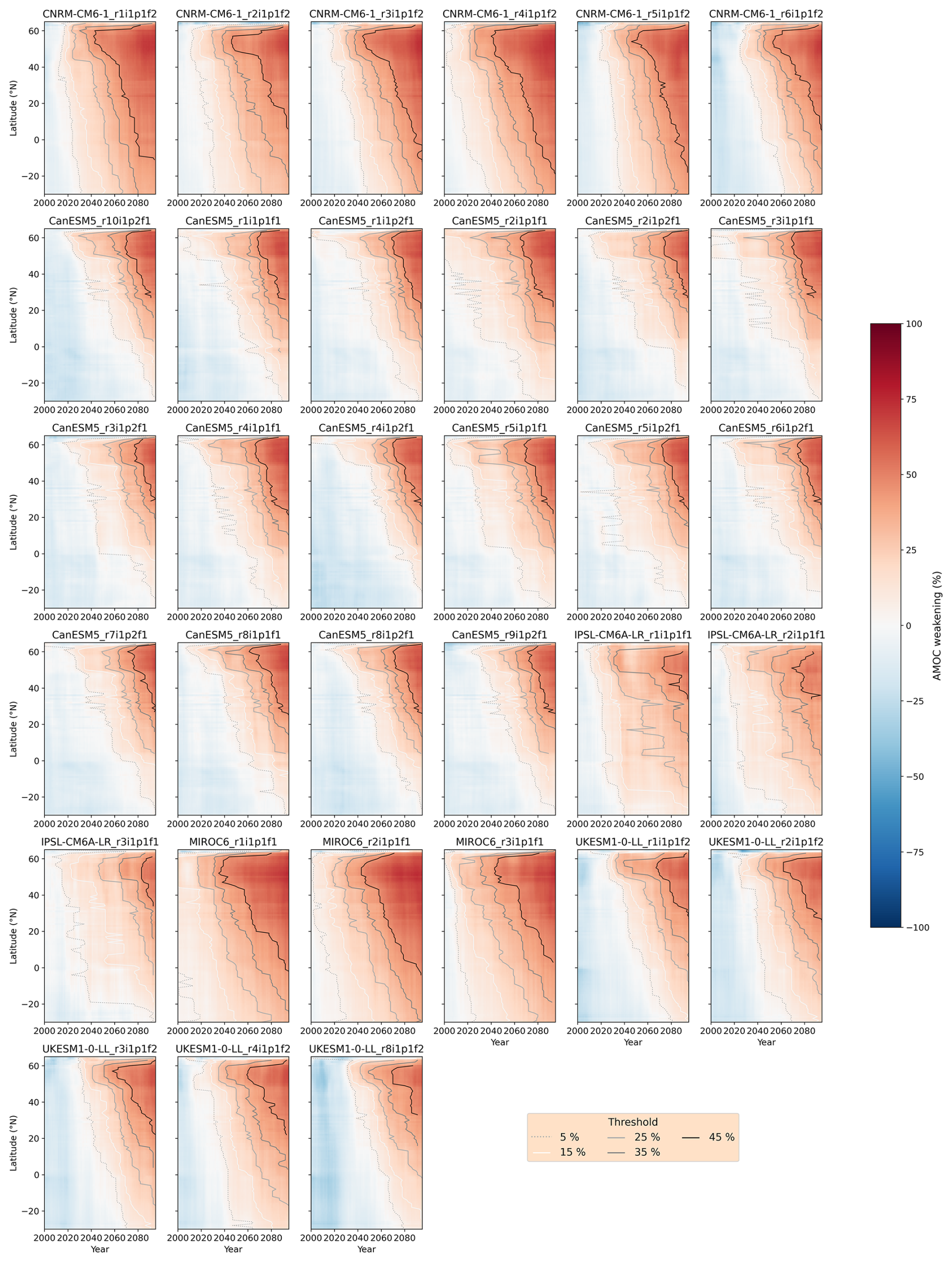
The full model set Hovmöller and weakening gradient plots for depth-space.

Figure E1 Weakening Hovmöller in depth-space for ssp585.

Figure E2 Weakening Hovmöller in depth-space for ssp126.

Figure E3 Weakening gradients in depth-space for ssp585.

Figure E4 Weakening gradients in depth-space for ssp126.

Figure E5 Weakening Hovmöller for individual ensemble members in depth-space for ssp585.

Appendix F: Fixed Latitude Model Timeseries

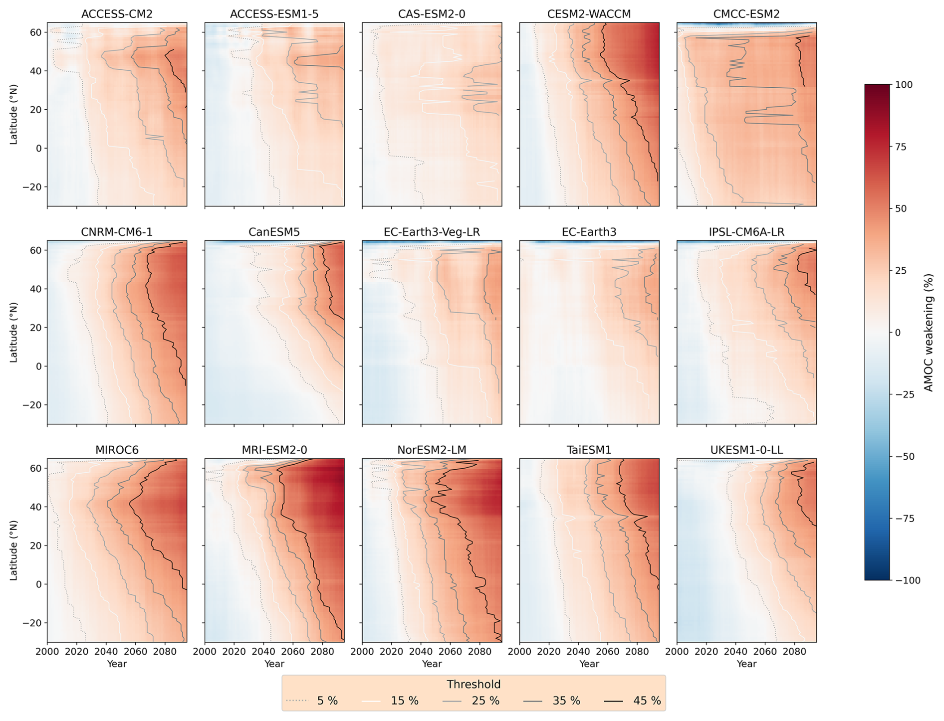
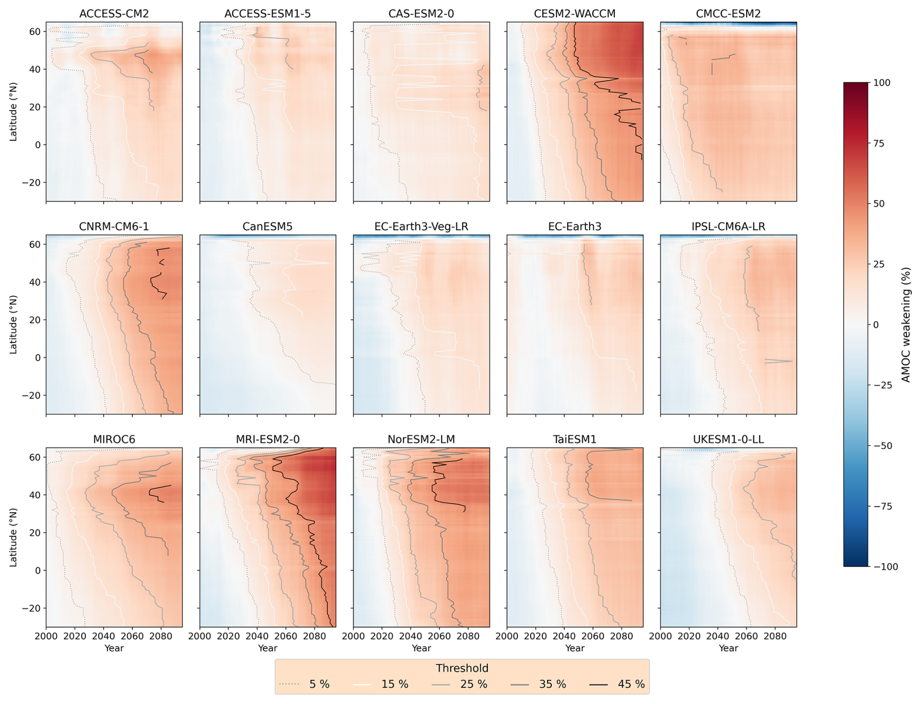
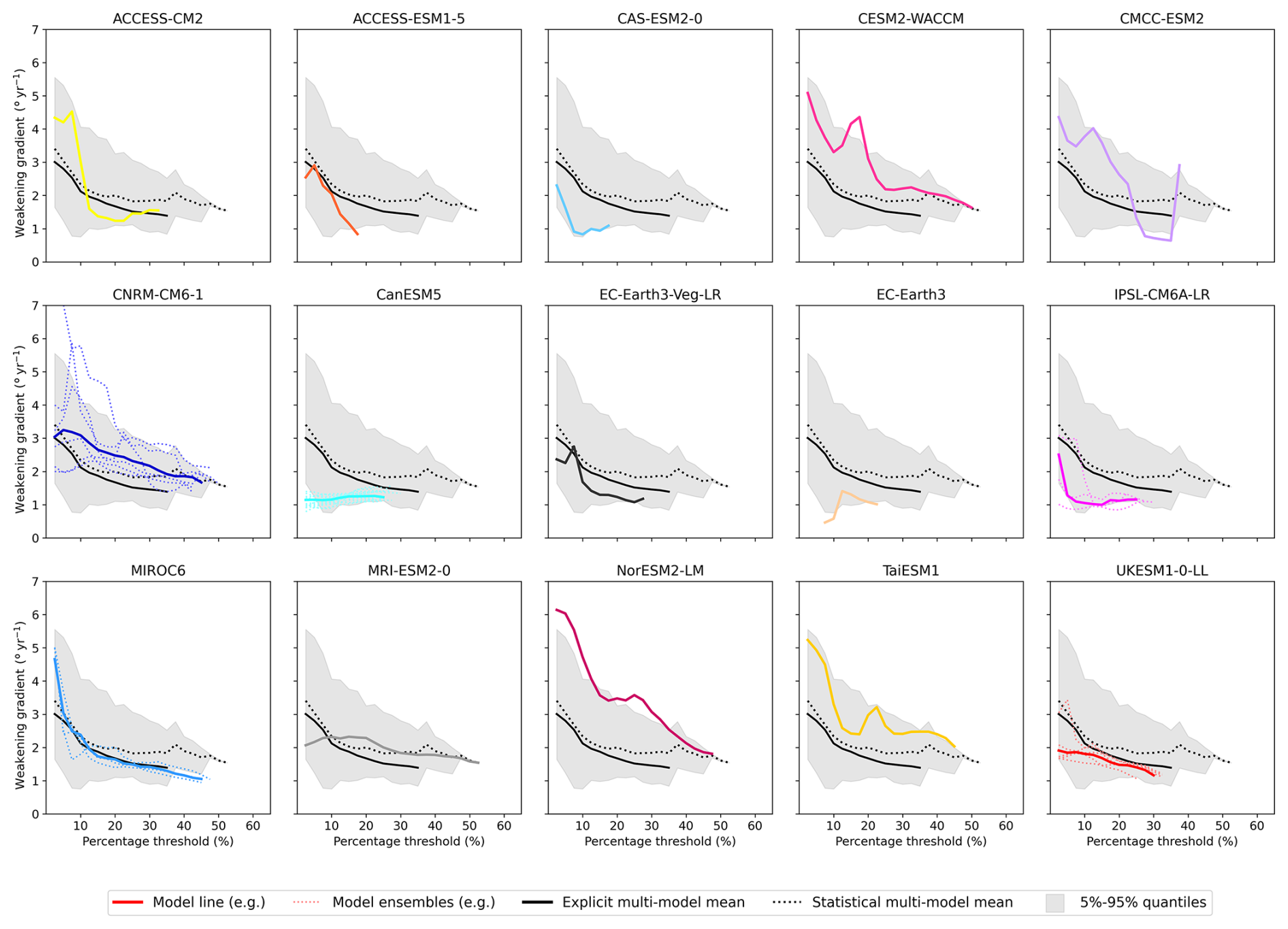
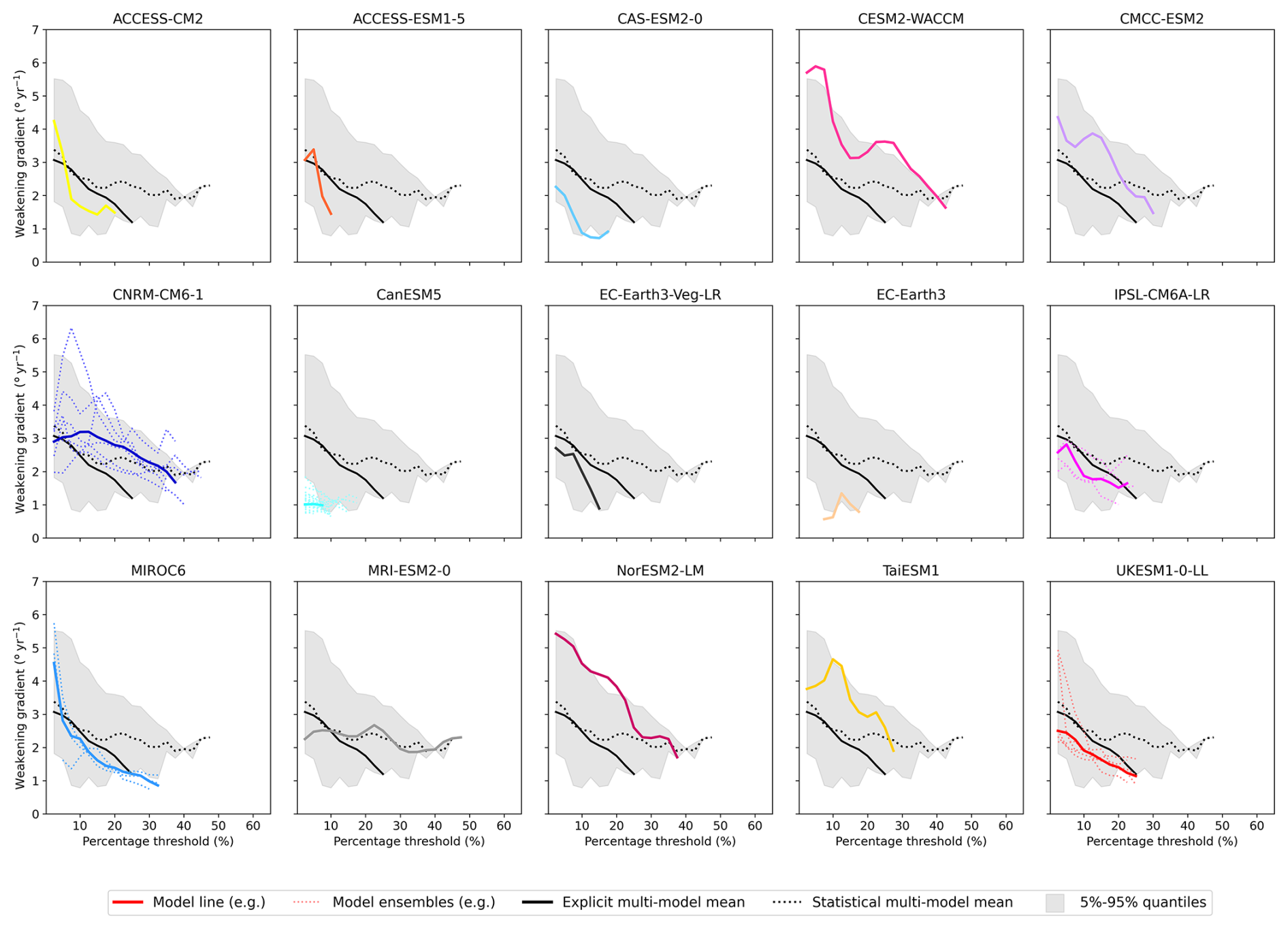
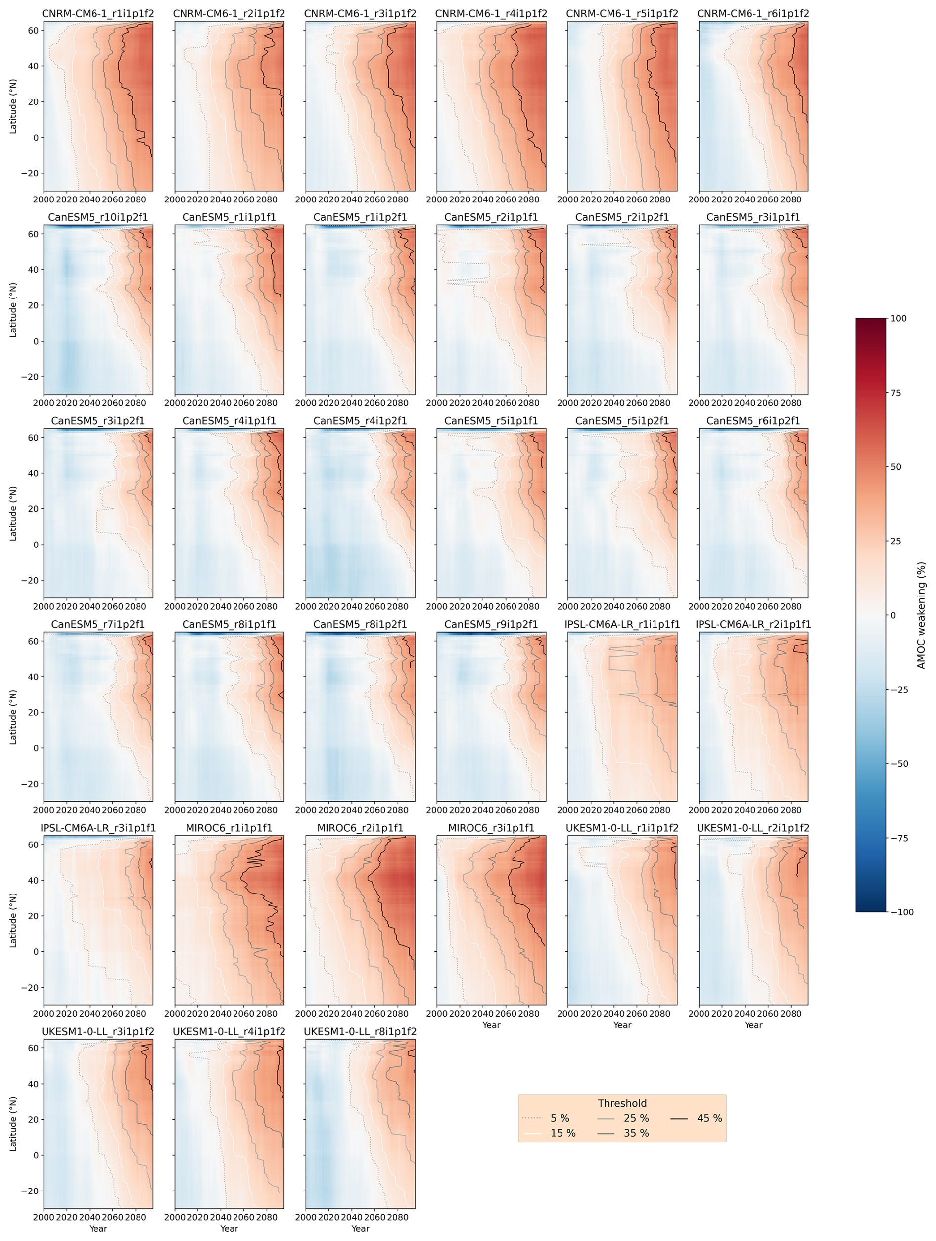
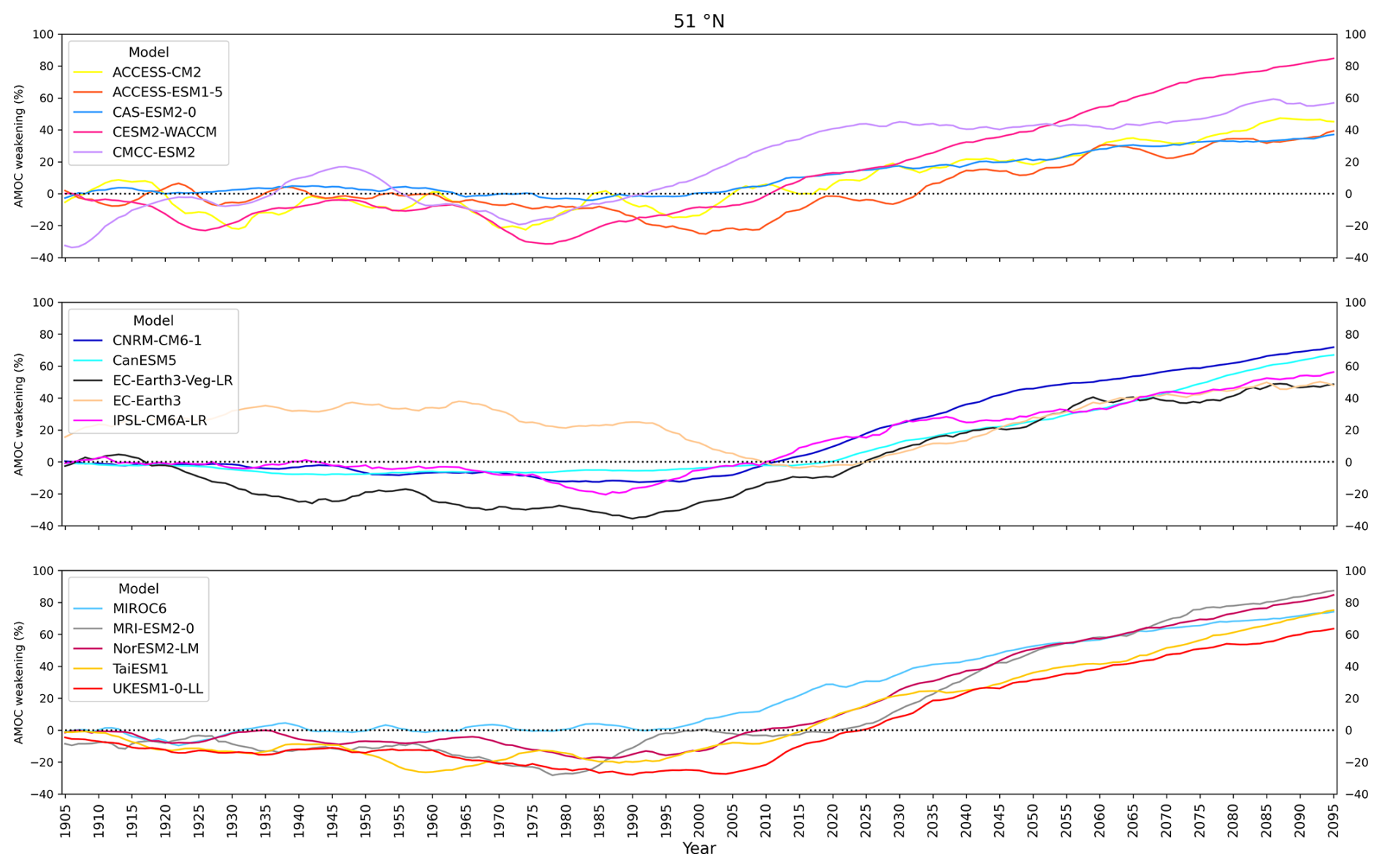
Figure F1 Timeseries of relative AMOC strength for the model set under historical and ssp585 forcing at 51° N. Calculated from the density-space streamfunction. AMOC strength relative to the mean 1850–1899 strength. The models are separated into groups of 5 for visual clarity. CanESM5, CNRM-CM6-1, IPSL-CM6A-LR, MIROC6 and UKESM1-0-LL are represented by their ensemble means.

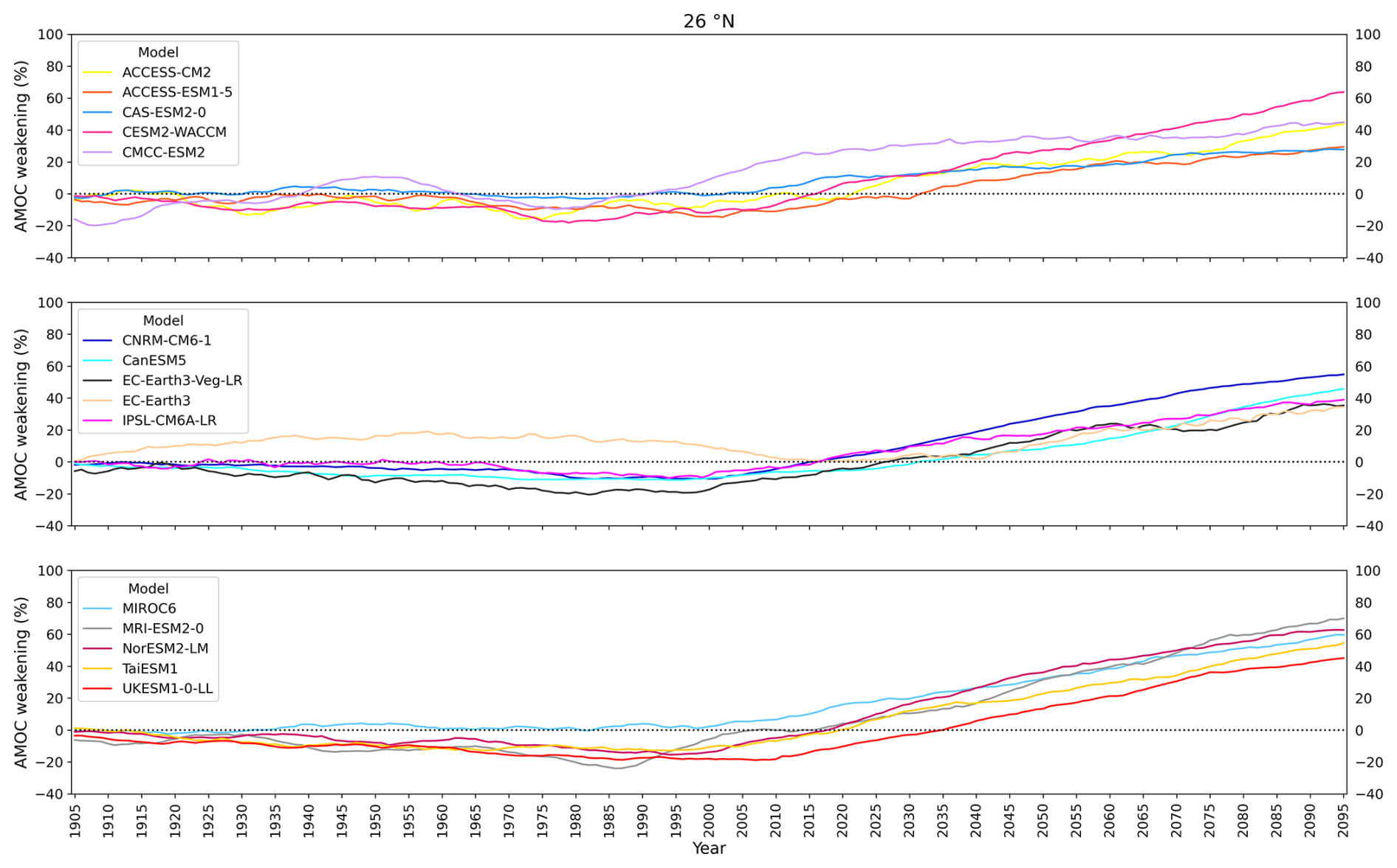
Figure F2 Timeseries of relative AMOC strength for the model set under historical and ssp585 forcing at 26° N. Calculated from the density-space streamfunction. AMOC strength relative to the mean 1850–1899 strength. The models are separated into groups of 5 for visual clarity. CanESM5, CNRM-CM6-1, IPSL-CM6A-LR, MIROC6 and UKESM1-0-LL are represented by their ensemble means.