An ensemble of regional CMIP3/CMIP5 wind wave scenarios for the North Sea and the Baltic Sea: a revisit

Storms and associated marine hazards pose environmental risks, particularly under long-term changes driven by anthropogenic climate change. This study assesses the potential impacts of future climate change on annual median and extreme significant wave height conditions in the North Sea and the Baltic Sea using an ensemble of up to 14 and 8 regional projections, respectively. The ensemble includes simulations based on IPCC CMIP3 and CMIP5 scenarios, incorporating a range of global and regional climate models, initial conditions, and emission scenarios to reflect diverse sources of uncertainty. High- and low-emission sub-ensembles were used to evaluate the influence of emission scenarios on projected significant wave height changes towards the end of the 21st century. Despite variations in magnitude and spatial patterns across the ensemble, some robust spatial and temporal trends emerge.

A meridional gradient of changes is simulated in the North Sea. Significant wave heights decrease along the western margins and increase in the east. These changes are more pronounced under high-emission scenarios, with median values decreasing by up to 5 % in the west and annual maxima increasing by over 5 % in the east. Time series analysis confirms these trends at selected locations, although there is still considerable internal variability among ensemble members.

In the Baltic Sea, both median and extreme wave heights are simulated to increase by more than 5 % in some areas. Although the response to emission scenarios is less distinct than in the North Sea, high-emission scenarios still yield more pronounced increases. Temporal analysis reveals that simulated changes become statistically significant by mid-century in central areas and later in western regions.

The results indicate a robust increase in significant wave height in the eastern North Sea and many regions of the Baltic Sea, as well as a consistent decrease in the western North Sea, particularly under high-emission scenarios. However, these trends are superimposed on substantial temporal and internal variability, highlighting the importance of using ensemble-based assessments to evaluate future marine climate conditions.

1 Introduction

The North Sea and the Baltic Sea in Northern Europe are important regions for many coastal and offshore activities, such as coastal protection, shipping, and planning and operating wind farms and oil or gas platforms. These activities are highly sensitive to mean and extreme sea states, particularly water levels and waves generated by wind, which can vary significantly under different atmospheric conditions. Therefore, it is crucial to understand long-term trends and future changes in the climate of wind, waves and water levels for coastal management and infrastructure planning (e.g. Weisse et al., 2015; Toimil et al., 2020; Meier et al., 2022).

Simulations of potential future changes in wave climate began in the 1990s with time-slice experiments based on single climate scenarios (e.g., WASA-Group, 1998). Since then, studies have increasingly addressed uncertainties in projections by incorporating multiple greenhouse gas emission scenarios and using ensembles of global climate models (GCMs) and regional climate models (RCMs). With the increasing computational capabilities, transient simulations, which often span from the mid-20th century to the end of the 21st century, aim to capture long-term trends and decadal variability in global (e.g. Wang and Swail, 2006; Hemer et al., 2013; Morim et al., 2020; Meucci et al., 2024) and regional wave conditions.

Regional-scale studies have become a focus due to the localised nature of coastal risks and infrastructure needs. In Europe, scenario-based wave climate projections have been conducted among others, in the North Sea (e.g., Debernard and Røed, 2008; Grabemann and Weisse, 2008; Lowe et al., 2009; de Winter et al., 2012; Groll et al., 2014a), in the Baltic Sea (e.g., Dreier et al., 2015; Groll et al., 2017; Soomere, 2023), or in both seas (Bonaduce et al., 2019). While early studies were often based on one or a few climate projections, more recent work increasingly relies on multi-member ensembles to improve robustness and capture the range of possible future conditions (e.g. Grabemann et al., 2015; Aarnes et al., 2017).

Revisiting the work of Grabemann et al. (2015) in the North Sea and Groll et al. (2017) in the Baltic Sea, this study evaluates changes in the significant wave height based on an updated and expanded ensemble of regional wave climate projections. While the earlier studies relied on atmospheric forcing from the Coupled Model Intercomparison Project Phase 3 (CMIP3) simulations (Meehl et al., 2007), the present work incorporates additional projections driven by CMIP5 simulations (Taylor et al., 2012), thereby increasing the ensemble size. Although CMIP3 scenarios are often viewed as outdated, they remain valuable in ensemble-based analyses. Their inclusion helps capture a wider range of plausible futures and offers important context for evaluating model robustness and climate sensitivity. By extending the limited number of regional wave projections, the greater ensemble allows to be subdivided into larger sub-ensembles of high- and low-emission scenarios. This enables a more detailed analysis of the effects of emissions on the significant wave height.

A key contribution of this study is the consistent comparison of regional wave climate responses across different emission pathways. Applying a unified analysis method across all scenarios provides a robust basis for interpreting projected changes in significant wave height conditions in both the North Sea and the Baltic Sea. Although changes in other wave parameters, such as period and direction, can have a significant impact on e.g. coastal erosion and protection, this study focuses on changes in significant wave height.

The atmospheric forcing ensemble accounts for multiple sources of uncertainty, including differences in emission scenarios, climate model formulations (via GCM–RCM combinations), and internal variability (through varying initial conditions). However, the simulations do not account for sea-level rise or changes in coastal bathymetry, both of which can also influence wave dynamics (e.g. Serafin et al., 2019; Chaigneau et al., 2023). Following the approach from Tebaldi and Knutti (2007) and Knutti et al. (2010) of “ensemble of opportunity”, and studies showing that possible weighting of ensemble members based on the historical performance does not necessarily lead to more robust future projections (e.g. Weigel et al., 2010), hence we treat every member of the ensemble as equal plausible and introduce no kind of weighting. This study specifically assesses whether significant differences in projected significant wave height arise between high- and low-emission scenarios. By combining CMIP3 and CMIP5-based projections into one ensemble, the analysis provides a better estimate on the range of uncertainty in future significant wave height conditions for the North Sea and Baltic Sea.

2 Data, models and statistical analyses

2.1 Ensemble members

This study uses an ensemble of 14 simulations of future wave climate projections for the North Sea and eight simulations for the Baltic Sea, along with their respective control simulations. These projections are based on atmospheric forcing derived from regionalised CMIP3 and CMIP5 simulations. The global climate simulations were produced using various GCMs. RCMs were used to downscale the output of the GCMs in order to generate higher-resolution atmospheric fields in the target regions. These atmospheric simulations were then used to drive the wave model WAM, which computed the sea state parameters for the North Sea and Baltic Sea.

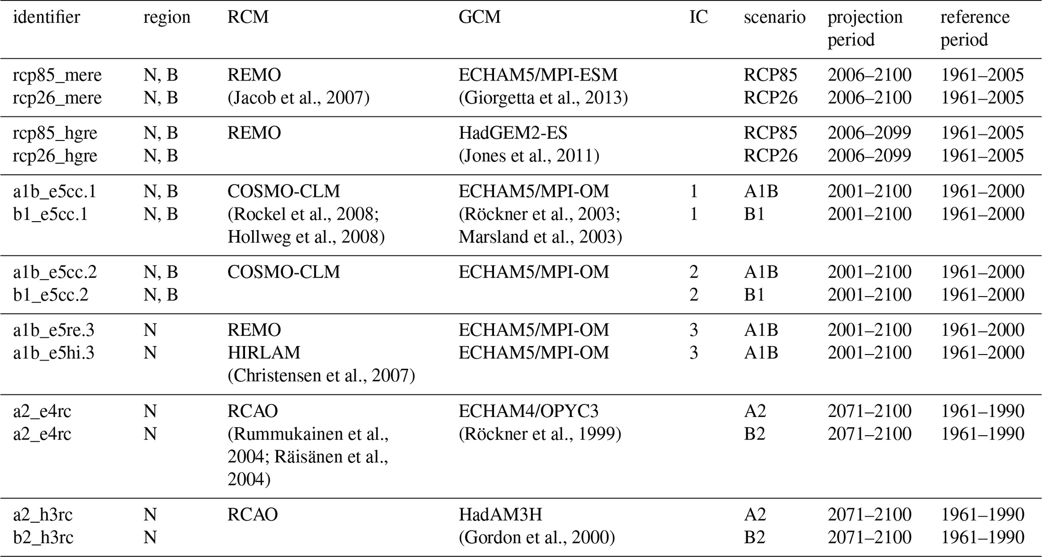
For the North Sea, the ensemble includes: four time-slice simulations (1961–1990 and 2071–2100; Grabemann and Weisse, 2008) and ten transient simulations (1961–2100). When combining time-slice experiments and transient simulations into one ensemble, it is important to use the same time period as given by the time-slice experiments. Additionally, we only use time-slice experiments for the spatial comparison of 30-year mean statistical values. Therefore, the influence of transient internal variability is expected to be reduced, making the combination of time-slice and transient simulations suitable for the spatial comparison conducted here. The transient simulations include six CMIP3–based simulations (Groll et al., 2014a, b) and four CMIP5–based simulations (Groll, 2025). For the Baltic Sea, all eight simulations are transient (1961–2100), and are split evenly between four CMIP3–based simulations (Groll et al., 2017) and four CMIP5–based simulations (Groll, 2025). Note that, for simplicity, we refer to 2100 as the end year of all simulations, even though the simulation periods for rcp85_hgre and rcp26_hgre terminate in 2099. Further details, including the simulation time spans, underlying GCM–RCM combinations, emission scenarios, and spatial domains, are provided in Table 1. To analyze different impacts of high and low emission scenarios, the total ensemble is split into two sub-ensembles, based on their global CO₂ concentraion in the year 2100. Above a CO₂ concentraion of 700 ppm the scenarios are sorted to high-emission scenarios, and below 700 ppm into low-emission scenarios. Concentration pathways for SRES scenarios (B1, B2, A1B, A2) were taken from the IPCC SRES framework (Prentice et al., 2001). Concentration pathways for RCP2.6 and RCP8.5 were taken from Meinshausen et al. (2011) and van Vuuren et al. (2011). The “high-emission” group comprises A1B, A2 and RCP8.5, which reach significantly higher concentrations and stronger radiative forcings. Although A1B represents a medium-emission scenario in the original SRES classification, it was assigned to the high-emission group due to its CO₂ concentrations of over 700 ppm by 2100. The “low-emission” group comprises RCP2.6, B1 and B2, which are characterised by comparatively low greenhouse gas concentrations and moderate radiative forcing up to the year 2100.

(Jacob et al., 2007)(Giorgetta et al., 2013)(Jones et al., 2011)(Rockel et al., 2008; Hollweg et al., 2008)(Röckner et al., 2003; Marsland et al., 2003)(Christensen et al., 2007)(Rummukainen et al., 2004; Räisänen et al., 2004)(Röckner et al., 1999)(Gordon et al., 2000)

Table 1 Summary of all simulations used in the total ensemble and for which region (North Sea – N; Baltic Sea – B) they are available. The four ensemble members based on the scenarios RCP8.5 and RCP2.6 differ in their underlying GCMs for the global climate. The six members based on the scenarios A1B and B1 differ in their underlying RCMs and initial conditions (IC) and the four members based on the scenarios A2 and B2 differ in their underlying GCMs. The simulation identifiers consists of two to three letters before the underscore presenting the respective scenarios. The four letters after the underscore describe the GCMs (me, he, e5, e4 and h3) and RCMs (re, cc, hi and rc), and the numbers after the point show the initial conditions in the case of the members with three different initial conditions.

2.2 Wave model and set-up

The third-generation spectral wave model WAM (WAMDI-Group, 1988), was used to simulate wave conditions. Previous studies have shown that for the CMIP3 simulations the model is capable of representing the historical climate (e.g., Weisse and Günther, 2007; Groll et al., 2014a, 2017). A verification of the CMIP5 simulations is presented in the Appendix B. The sea state was simulated using different versions of WAM in a nested mode, with a coarse grid simulation covering parts of the northeastern Atlantic, the North Sea and the Baltic Sea, with a horizontal resolution of 0.5° × 0.75° (latitude × longitude) which corresponds to about 50 km × 50 km. This area is large enough to take into account swell and wind sea entering the North Sea from the North Atlantic. The fine-grid simulations for the North and Baltic Sea received spectral boundary conditions from the coarse-grid simulations. The horizontal resolution of the fine grid simulations is about 5 km × 5 km. More details on the horizontal and spectral resolution as well as the domain borders can be found in Table 2, the domains are displayed in Fig. 1. In the Baltic Sea, sea ice was accounted for by setting the wave spectra to missing values where grid cells were ice-covered, based on monthly sea ice coverage from the respective GCMs. All simulations were run in shallow water mode with depth refraction and depth-induced wave breaking enabled. All coarse grid simulations were forced with three hourly wind and fine grid simulations with hourly wind fields.

Grabemann and Weisse (2008)Groll et al. (2014a, b)Groll et al. (2017)Groll (2025)

Table 2 Model domains, spatial and spectral resolution of the different used versions of the wave model WAM together with references.

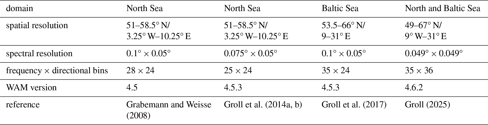
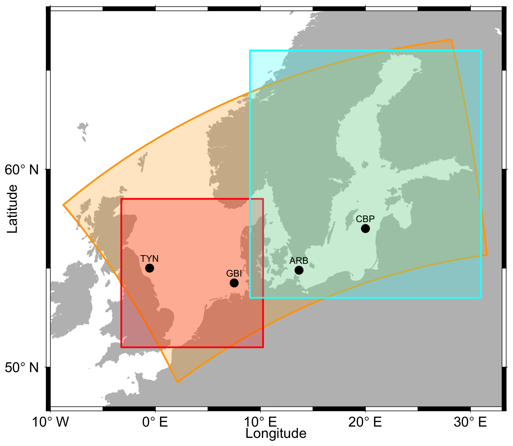
Figure 1 Model domain of the fine grid simulations for the North Sea and the Baltic Sea (orange border) together with the domains for which results are shown for the North Sea (red border) and the Baltic Sea (cyan border). The four chosen locations for the time series analysis are identified by black circles and abbreviations.

2.3 Statistical analysis

To quantify future changes in wave climate, wave statistics were computed at each grid point from the hourly model output, as annual maximum, annual 99th percentile and annual median of the significant wave height (SWH). These annual values were then averaged over 30-year running periods (1961–1990 to 2071–2100). In the following, all 30-year values are only indicated with the term maximum, 99th percentile and median, respectively. The climate change signal is defined as the difference between a future 30-year time slice and the reference period (1961–1990). The period 1961–1990 is retained as the reference to allow for direct comparison with the older studies (Grabemann and Weisse, 2008; Groll et al., 2014a, b, 2017), and because it is the only common baseline available for the time slice projections. Note that, as the different model simulations are conducted on slightly different model grids, all simulations are first interpolated onto the same grid prior to analysis.

Future changes in SWH will be discussed based on spatial and temporal variability.

• Spatial variability: The climate change signal for the period 2071–2100 compared to the period 1961–1990 was derived. A common climate change signal is defined as the number of ensemble members at a given grid point that exhibit a consistent magnitude of change. A one-sided exact binomial test was applied to assess whether the observed number of agreeing ensemble members (N) is significantly greater than expected by random chance (with a null probability of success p = 0.5). Agreement was evaluated for various change thresholds (0 %, 2.5 %, 5 %, and 7.5 %), and statistical significance was assessed at the 0.05 level. Specifically, a signal is considered significant if at least 11 out of 14 ensemble members agree in the North Sea or at least seven out of eight agree in the Baltic Sea. To maintain the same confidence level, the required number of agreeing members was adjusted for sub-ensembles representing different emission scenarios: at least seven out of eight for the high-emission North Sea sub-ensemble, six out of six for the low-emission North Sea sub-ensemble, and four out of four for both the high- and low-emission Baltic Sea sub-ensembles.

• Temporal variability: The 30-year running means of the SWH climate change signal are evaluated for the period 1961–1990 to 2071–2100 at two locations in the North Sea (German Bight and Tyne; see Fig. 1) and two in the Baltic Sea (Arkona Basin and Central Baltic Proper; see Fig. 1). This analysis is conducted separately for high-emission and low-emission sub-ensembles, with the ensemble median used to represent each sub-ensemble. The median is chosen for its robustness to outliers. The North Sea sub-ensembles consist of six high-emission and four low-emission members, while the Baltic Sea sub-ensembles include four members in each category. To assess whether temporal changes in the 30-year running means are statistically significant relative to the reference period (1961–1990), we apply the non-parametric Mann–Whitney U test and the statistical significance was assessed at the 0.05 level. The test is performed using all annual SWH values from the ensemble members within each 30-year window, rather than comparing only aggregated medians. This approach ensures that the full distribution of annual values is considered and accommodates potential non-normality in the data.

3 Results

In the following the spatial and temporal variability of the future wave climate projections of the SWH for the North Sea and the Baltic Sea will be discussed. Whereas for the spatial changes only the last 30 years of the 21 century are taken into account, the temporal variability of changes is discussed on 30-year running means for the whole simulation period, when transient simulations are available. The analysis of the temporal variability is done for two locations in both the North Sea and the Baltic Sea.

3.1 Spatial Variability

3.1.1 North Sea

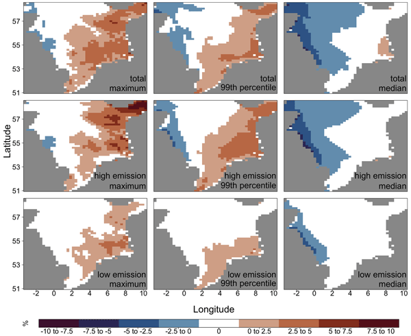
The total ensemble for the North Sea includes 14 wave climate simulations, ten transient and four time-slice experiments. To indicate a statistically significant change, at least 11 of these simulations must exhibit the same magnitude of relative change. The common climate change signal in the North Sea generally shows a west-to-east gradient of changes in SWH (Fig. 2), with the largest increases occurring in the eastern part of the North Sea and the largest decreases in the western part.

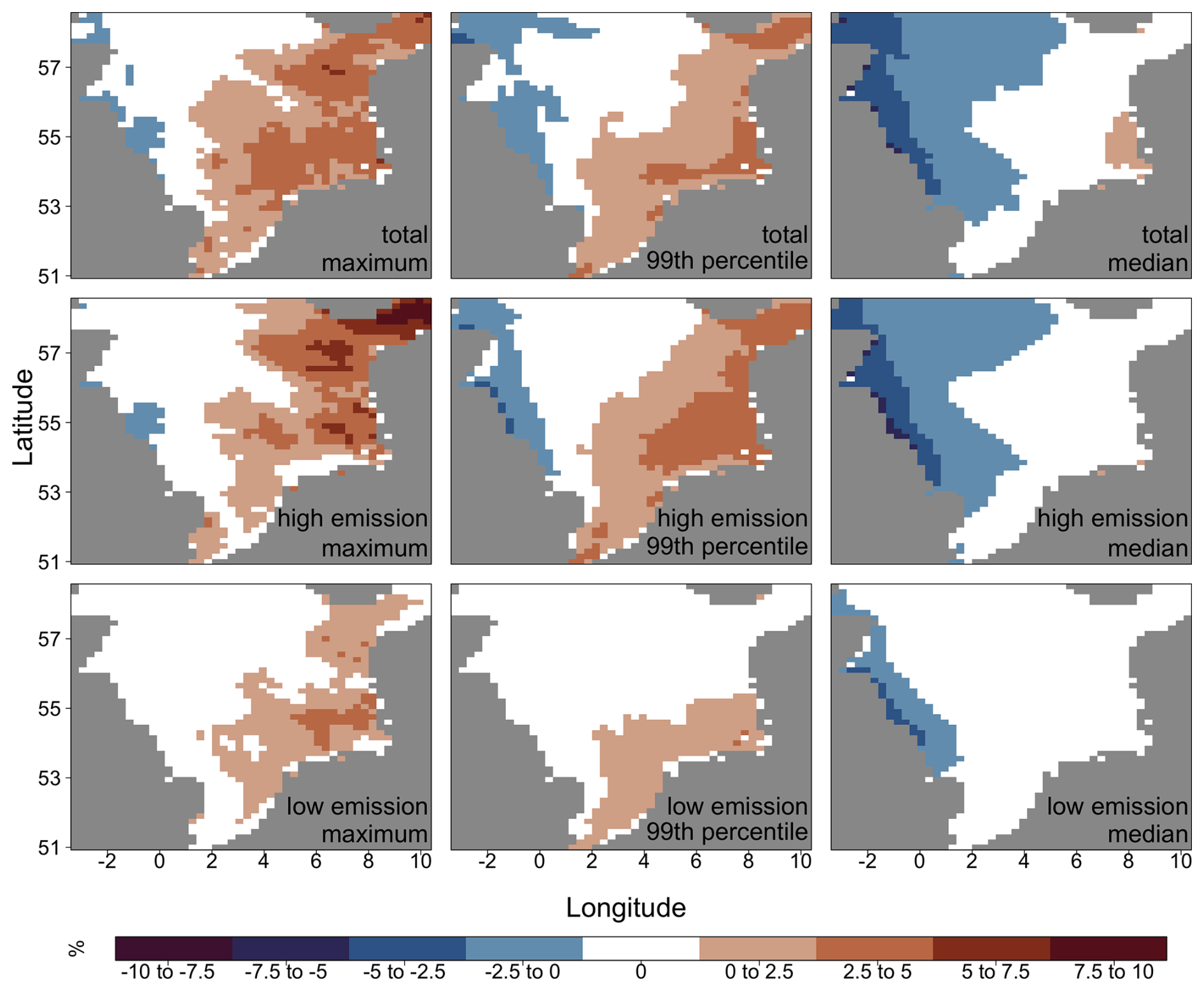
Figure 2 Common climate change for maximum (left), 99th percentile (middle) and median (right) SWH in the North Sea for the last 30 years of the 21st century: relative change in SWH for the total ensemble (upper row) and for the high emission (middle row) and low emission (bottom row) sub-ensembles. For the total ensemble at least 11 out of 14 members are taken into account, for the high (low) emission sub-ensembles seven (six) out of eight (six) members are included.

The common changes in the maximum SWH show a large area of increase from the south over the central parts up to the Skagerrak, with increases exceeding 5 % in the German Bight and in the Skagerrak at few grid points. Conversely, in a few areas along the British coast, a small decrease of up to 2.5 % can be seen. No common change is evident in northern parts of the North Sea. The same spatial characteristics apply to the common changes in the 99th percentile SWH, but the areas and the amplitudes of the common increase are slightly smaller. In the eastern an northern parts of the North Sea the increase ranges only between 2.5 % and 5 %. In contrast, then common decrease along the British coast are covering a larger areas but only exceed 2.5 % in a small region. No common change is evident in the central and northern parts of the North Sea. Common changes in the median SWH changes show decreases of up to 5 % along the British coast, and increases of less than 2.5 % in a small area in the north western part of the German Bight. There is no evidence of any significant common change from the southern North Sea to the Skagerrak in the north.

Until now, all ensemble members were treated as equally likely, regardless of the emission scenario. To distinguish the impacts between high and low emission scenarios the total ensemble was split into a high and a low emission sub-ensemble. The overall spatial distribution of the common changes for both sub-ensembles is the same as when all scenarios are considered. However, the changes are more pronounced and cover a larger area when only the high-emission scenarios are considered (Fig. 2, middle row).

The maximum SWH shows larger differences in the common increases of the high emission sub-ensemble compared to using the total ensemble, with larger areas above 5 % and even 7.5 % in the Skagerrak. Only a small region in the west shows a common decrease. The 99th percentile SWH also shows a comparable area in the east with a common increase in the high-emission sub-ensemble, but the magnitude of the increase is never above 5 %. In contrast, the area of decrease in the western North Sea is larger than the changes in maximum SWH, reaching over 2.5 % at some grid points. The median SWH decrease is similar to that found when considering all scenarios, with a maximum decrease of approximately 5 % occurring in small areas along the British coast. However, no common increase can be found for the median SWH in the eastern part of the North Sea. Changes using only low emission scenarios show smaller areas and amplitudes than changes using all or only high emission scenarios. The maximum SWH shows a common increase of more than 2.5 % in some areas in the east, whereas the 99th percentile SWH for low emission scenarios is almost always below 2.5 %. Neither extreme SWH measure shows any areas of common decrease in the east. The median SWH shows a decrease in a small area in the west of slightly below 2.5 %, with no common increases in the east.

3.1.2 Baltic Sea

The total ensemble for the Baltic Sea consists of eight wave climate simulations. To demonstrate a statistically significant change, at least seven out of the eight simulations must show the same amount of relative change. Changes in the maximum SWH of the total ensemble members indicate an increase in the 30-year mean in many areas of the Baltic Sea (Fig. 3). The largest common changes can be found in the central Baltic Proper, the Gulf of Riga, the Gulf of Finland, and a small area to the west of Bornholm, with an increase exceeding 5 %. Larger areas show a common increase of between 2.5 % and 5 %, from the Skagerrak and Kattegat to the south of Sweden, covering large parts of the central Baltic Proper, the Gulf of Riga and the Gulf of Finland, as well as some areas in the Bothnian Sea and Bay. Changes in the 30-year mean of the 99th percentile SWH show a more homogeneous increase over large areas of the Baltic Sea; however, only a small area in the southeast of the Baltic Sea shows an increase of more than 5 %. Increases of up to 5 % in the 30-year mean of the median SWH are mostly limited to the regions of the Bothnian Sea and Bay and the Gulf of Finland that are covered by seasonal ice.

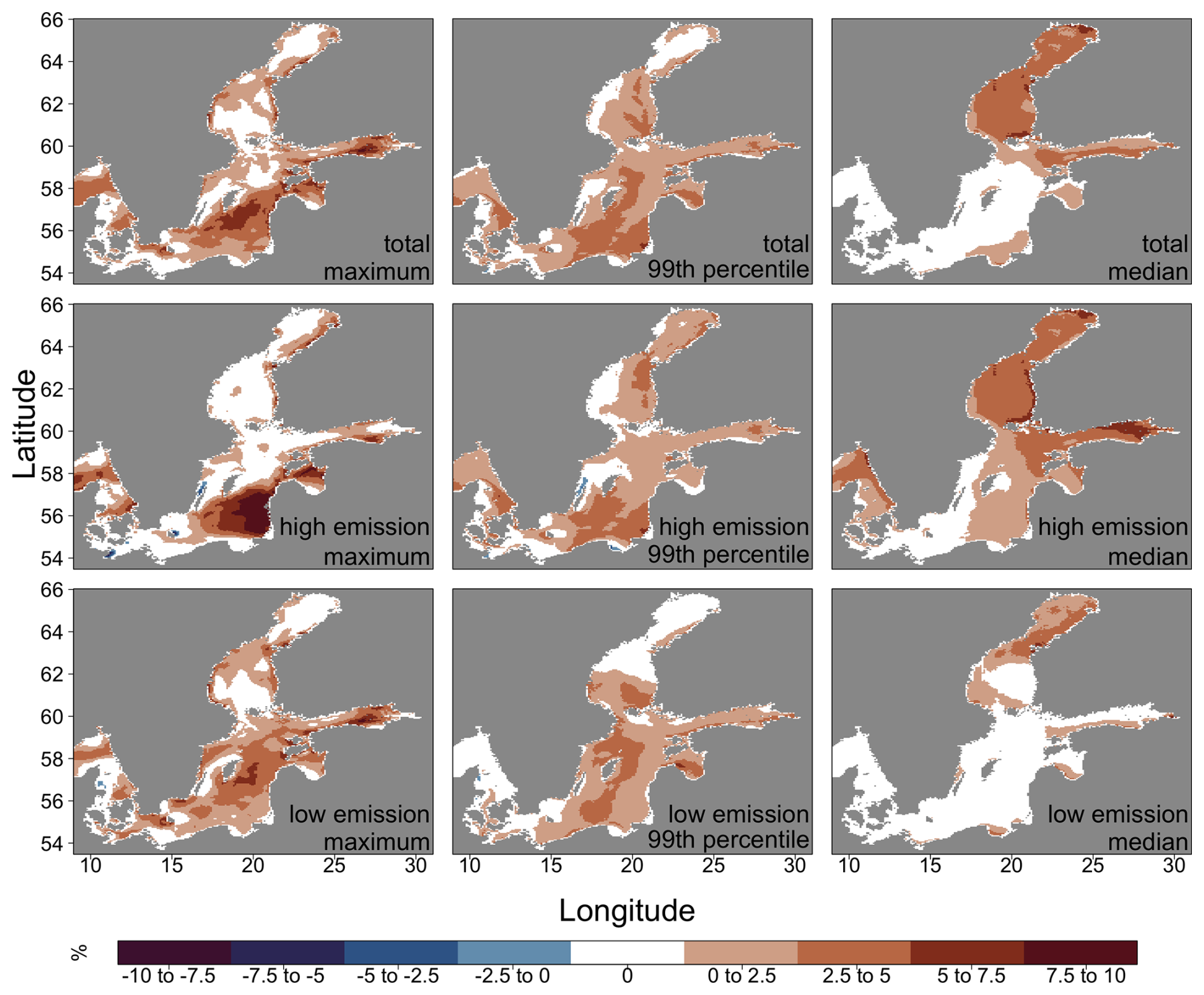
Figure 3 Common climate change for maximum (left), 99th percentile (middle) and median (right) SWH in the Baltic Sea for the last 30 years of the 21st century: relative change in SWH for the total ensemble (upper row) and for the high emission (middle row) and low emission (bottom row) sub-ensembles. For the total ensemble at least 7 out of 8 members are taken into account, for the high or low emission sub-ensembles four out of four members are included.

As each sub-ensemble of high and low emission scenario simulations consists of four members, all members must show at least the same amount of relative change to be considered statistically significant. The high emission scenarios show a common increase of more than 7.5 % in the 30-year mean of the maximum SWH over a large area of the central Baltic Proper and a smaller area of the Gulf of Riga. Areas with an increase of more than 5 % can be found in the Kattegat, the central Baltic Proper, the Gulf of Riga and the Gulf of Finland. Smaller increases of less than 2.5 % can be found in several areas across the Baltic Sea. Small areas east of Bornholm, between Öland and the Swedish mainland, and in the south-western part of the Baltic Sea show a decrease in the 30-year mean of the maximum SWH in all four simulations. Changes in the 99th percentile SWH for the high emission scenarios are comparable to those in the maximum: larger areas experience an increase, albeit smaller, with increases of more than 5 % only occurring in the south-eastern tip of the Baltic Sea. The median SWH increases over most regions of the Baltic Sea, except regions in the south-western parts between Sweden and the Polish and German coasts. In the seasonal ice-covered regions of the Bothnian Sea and Bay, as well as in the Gulf of Finland, the median SWH increases by 2.5 % and even 5 %. The increase is also above 2.5 % in the eastern parts of the Kattegat.

Changes in the low emission scenarios show comparable characteristics, with a smaller overall increase and not necessarily smaller areas. The changes in median SWH mostly affect the Bothnian Bay, with an increase of more than 2.5 %. This indicates that the low emission scenarios show comparable changes, but with a lower amplitude than the high emission scenarios.

3.2 Temporal Variability

The temporal variability of changes in SWH is illustrated using time series of the 30-year running means of maximums, 99th percentiles and medians of SWH for each selected location in the North Sea and in the Baltic Sea from 1961 to 2100, relative to the reference period (1961–1990). Only the transient ensemble members are considered. In addition to the temporal variability of individual ensemble members, the temporal variability of the mean across high and low emission scenarios is also discussed.

Grabemann et al. (2015) verified that the climate projections based on the emission scenarios A1B and B1 display a realistic variability of the 30-year running means of the area-averaged maximum SWH for the North Sea and the reference period 1961 to 1990. This was established by comparing respective time spans and two locations of a hindcast from 1958 to 2002 (Weisse and Günther, 2007). This comparison showed that the variability at the beginning of the A1B and B1 North Sea ensemble members was within the variability derived from the hindcast.

3.2.1 North Sea

At the German Bight (GBI) location (Fig. 4, left), the individual members of the 30-year running mean of the maximum SWH show considerable variability within the ensemble. While most members exhibit a relatively small but stable increase towards the end of the 21st century, some show greater temporal variation, with increases of up to 10 %, and above, compared to the reference period. A few members show a decreasing trend, with only one displaying a consistent decline of about 9 % towards the end of the simulation period. To reduce variability and obtain more robust estimates, ensemble medians for the high- and low-emission sub-ensembles are calculated. Compared to the individual members, these sub-ensemble medians show much lower interdecadal variability. Although neither exhibits a consistent upward trend throughout the 21st century, both ensemble medians show an increase towards the end.The high-emission sub-ensemble also showed a statistically significant increase in the middle of the simulation period, demonstrating a rise of over 8 %. Both ensembles showed an increase of around 5 % towards the end of the simulation period, but only the increase for the high-emission sub-ensemble is statistically significant. The 30-year running mean of the 99th percentile SWH shows less temporal and ensemble variability across individual members. Only one member deviates significantly, showing a pronounced increase during the second half of the century. The median for the high-emission sub-ensemble again shows a larger and statistically significant increase of more than 5 % by the end of the century. The ensemble median for the low-emission sub-ensemble also shows an increase, though smaller and not statistically significant. Only the changes in the 99th percentile SWH ensemble median under high-emission scenarios are statistically significant, indicating robust changes in SWH in the German Bight. By contrast, the sub-ensemble for low-emission scenarios exhibits no significant changes, suggesting that changes in the 99th percentile SWH at GBI are less robust. Ensemble variability is even lower for the 30-year running mean of the median SWH, with the exception of one outlier. While the ensemble median of the high-emission sub-ensemble still shows a slight increase, the ensemble median of the low-emission sub-ensemble exhibits no significant changes at the GBI location. Neither the median SWH for the high- and low-emission sub-ensembles, nor the maximum and 99th percentile SWH for the low-emission sub-ensembles, shows statistically significant changes, implying that any trends are either too small to detect or are masked by substantial internal ensemble variability.

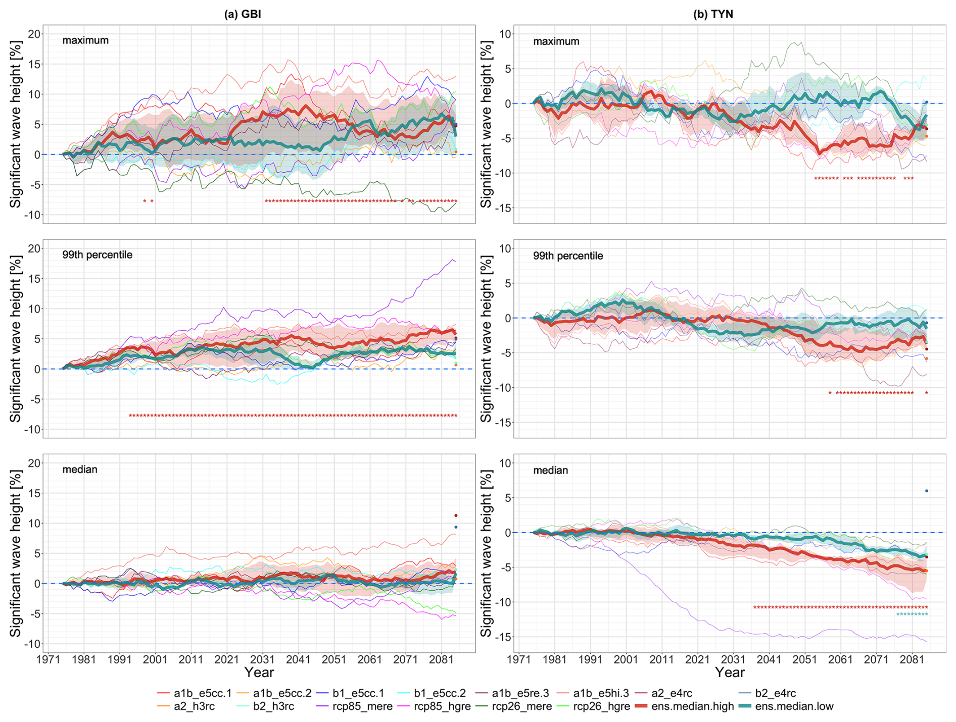
Figure 4 Time series of relative 30-year running means of the SWH climate change signal maximum (top), 99th percentile (middle) and median (bottom) from 1961–1990 to 2071–2100 for two locations in the North Sea (column a – German Bight-GBI; column b – Tyne-TYN). Single ensemble members are presented by thin lines. The median of the high(low)-emission sub-ensemble is shown as a thick red (blue) line. Red (blue) shadings presents the confidence interval (25 and 75 percentiles) of the sub-ensemble median. The statistical significance of the discussed changes to the ensemble median at the 0.05 level is indicated by an asterisk. For completeness, single points show the relative 30-year means of the SWH climate change signal of the four time slice experiments.

At the western location, Tyne (TYN), near the British coast, the results indicate a general tendency toward decreasing SWH, consistent with the patterns discussed in the previous section on spatial variability. While individual 30-year running means of maximum SWH show substantial variability throughout the simulation period, the ensemble medians for both high- and low-emission sub-ensembles fluctuate around the baseline. During the first half of the century, the 50 % confidence interval consistently encompasses the baseline, indicating no statistically significant changes. However, from around 2040 onward, the ensemble median for the high-emission sub-ensemble shows a statistically significant decreasing trend, continuing almost to the end of the 21st century. This decrease reaches a maximum of approximately 6 %, and around 3 % by the end. In contrast, the low-emission scenarios continue to vary around the baseline for most of the simulations, with a slight downward trend emerging in the final decade, though it never becomes statistically significant. The 30-year running mean of the 99th percentile SWH shows broadly similar characteristics to the maximum, albeit with less variability among individual ensemble members. The ensemble median for the high-emission sub-ensemble shows a nearly continuous, statistically significant decrease of about 4 %–5 % towards the end of the 21st century. The low-emission scenarios, meanwhile, show no statistically significant changes. For the 30-year running mean of the median SWH, variability within the ensemble is generally low, except for one outlier. A steady and statistically significant decrease in the ensemble median becomes evident from around 2030 under high-emission scenarios, reaching a decrease in SWH of approximately 5 % by the end. Low-emission scenarios also show a decreasing trend, beginning later, around 2060, and becoming statistically significant from the mid-2070s onward, reaching around 3 % by the end of the century.

3.2.2 Baltic Sea

At the western Baltic location (Arkona Basin – AB), the 30-year running mean of the maximum SWH across individual ensemble members exhibits multi-year to multi-decadal variability. While the sub-ensemble medians for both high- and low-emission scenarios indicate an overall increase towards the end of the 21st century, with embedded multi-decadal fluctuations of up to 4 %–5 %, these changes are not statistically significant throughout the simulation period. The 30-year running mean of the 99th percentile SWH shows less variability, both within individual members and across the ensemble, compared to the maximum SWH. Again, sub-ensemble medians indicate an increasing trend towards the end of the century. For high-emission scenarios, the ensemble median increase reaches approximately 4 %, which becomes statistically significant only in the final years of the simulation. Low-emission scenarios also show an increase, consistently smaller than that of the high-emission scenarios, except for a few isolated years. The ensemble median of the mean SWH reveals similar temporal variability, though with slightly less inter-member spread. Both sub-ensembles show an increasing trend. For low-emission scenarios, the median SWH increases significantly, up to 3 %, by mid-century, followed by a slight decline, yet remaining positive. However, due to greater spread within the sub-ensembles, these later changes are not statistically significant. In contrast, the median for the high-emission sub-ensemble remains consistently positive, with a statistically significant increase of approximately 5 % in the final two decades of the 21st century.

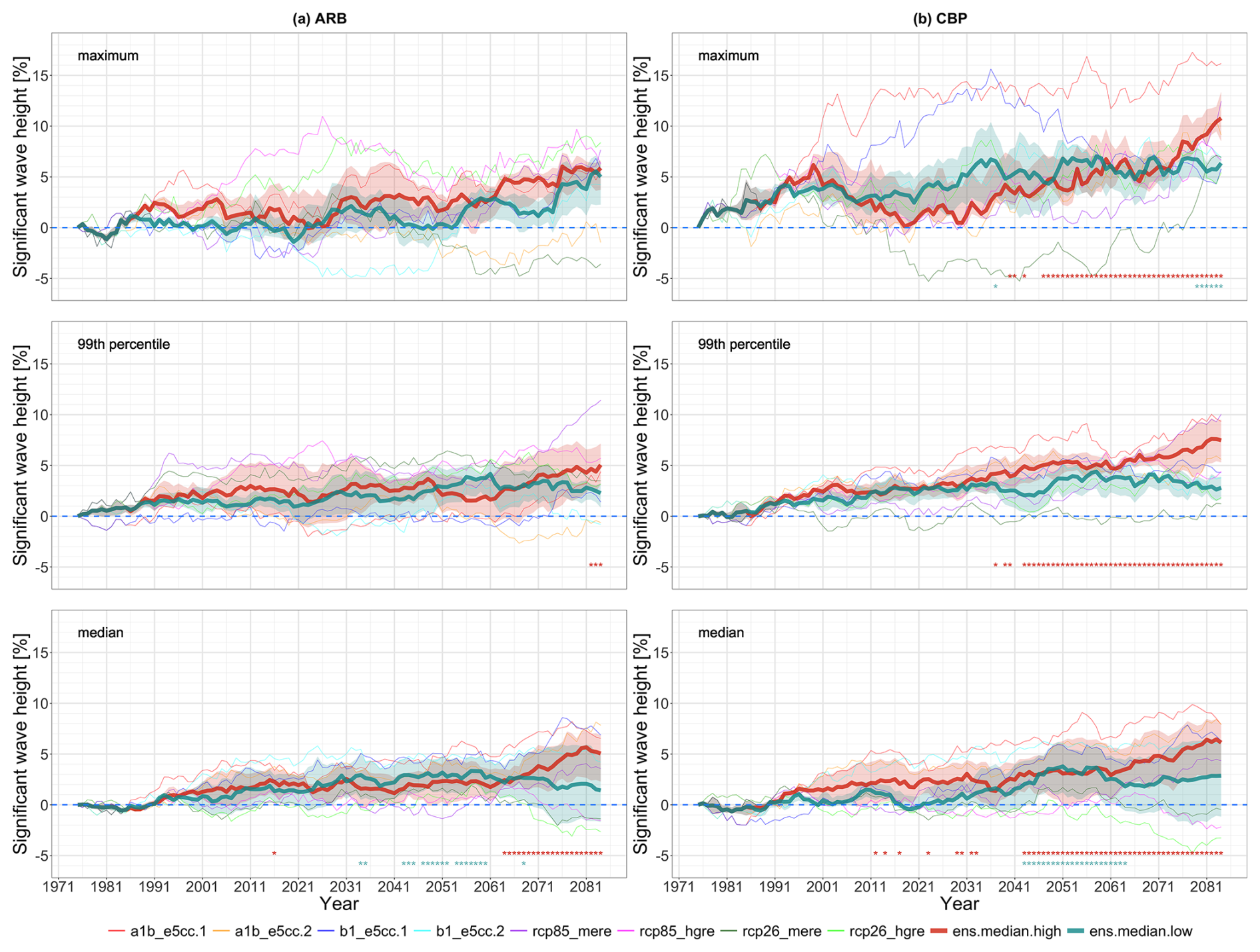
Figure 5 Time series of relative 30-year running means of the SWH climate change signal maximum (top), 99th percentile (middle) and median (bottom) from 1961–1990 to 2071–2100 for two locations in the Baltic Sea (column a – Arkona Basin-ARB; column b – Central Baltic Proper-CBP). Single ensemble members are presented by thin lines. The median of the high(low)-emission sub-ensemble is shown as a thick red (blue) line. Red (blue) shadings presents the confidence interval (25 and 75 percentiles) of the sub-ensemble median. The statistical significance of the discussed changes to the ensemble median at the 0.05 level is indicated by an asterisk.

At the Central Baltic Proper (CBP) location, the time series of the 30-year running mean maximum SWH exhibit substantial variability across individual ensemble members and within the ensemble. Some individual time series show a strong increase at the beginning of the 21st century, while others display a steadier rise towards the end of the 21st century or even a mid-century decrease followed by a late-century increase. The range of variability across individual members spans from −5 % to +17 %. The ensemble median for the high-emission sub-ensemble shows multi-decadal variability with a steady increase of up to 10 % by the end of the 21st century, which becomes statistically significant from mid-century onwards. In contrast, the ensemble median for the low-emission sub-ensemble shows a more gradual increase, reaching up to around 6 %. However, due to greater ensemble spread, these changes are only statistically significant at the end of the 21st century. The time series of 30-year running mean of the 99th percentile SWH at CBP exhibits much less multi-decadal variability than the maxima. While some individual ensemble members show increases of 8 %–9 %, others fluctuate around the baseline. Both high- and low-emission sub-ensembles show an almost linear increase up to mid-century. From there, the high-emission scenarios continue to rise, reaching increases of 5 %–6 % by 21st century's end, which are statistically significant. The low-emission scenarios, however, remain between 2 % and 4 %, with no statistically significant trend. The time series of the 30-year running mean of median SWH show slightly more variability among individual members than the 99th percentile, but the sub-ensemble medians for high and low emission scenarios reveal a relatively steady increase towards the end of the 21st century. For high-emission scenarios, the increase becomes statistically significant from mid-century onward, reaching about 5 %–6 %. The low-emission scenarios show a statistically significant increase of around 3 % by mid-century. However, this significance disappears afterwards due to increasing ensemble variability, despite the ensemble median remaining relatively stable.

4 Discussion and conclusion

Based on the ensemble of CMIP3- and CMIP5-driven wave projections analysed in this study, projected common changes in significant wave height towards the end of the 21st century reveal spatial patterns in both the North Sea and the Baltic Sea. In the North Sea, a west-to-east gradient emerges, with extreme SWH (maxima and 99th percentiles) is projected to increase by 2.5 % to 5 % mainly occurring in the eastern and southern regions. In contrast, the western and northern regions experience a projected decrease, particularly in median SWH (−2.5 % to −5 %). The Baltic Sea exhibits a more widespread projected increase in SWH. The ensemble suggests the largest changes in extreme SWH (maximum and 99th percentile) occur in the western, southern and central Baltic, with projected increases between 2.5 % and 7.5 %. Median SWH increases are projected to be more concentrated in the northern Baltic and are of a similar magnitude.

Even if the relative changes in median or extreme SWH are comparable, it should be noted that the absolute values differ and depend on the region in the North Sea and Baltic Sea. These values range from approximately ±10 cm for the median, −20 to +50 cm for the 99th percentile, and up to +1 m for the maximum SWH (see Appendix A for more details). Depending on the region and application, these differences could impact e.g. sediment transport, coastal erosion, coastal protection infrastructure, and offshore planning and safety in different ways.

The projected SWH patterns are broadly consistent with previously reported wind-related changes in the atmospheric forcing of the underlying CMIP3 and CMIP5 simulations and with findings from earlier studies based on the same or similar model ensembles. For a subset of the simulations used in this study, earlier analyses (Grabemann and Weisse, 2008; Gaslikova et al., 2013; Grabemann et al., 2015; Groll et al., 2017) revealed an increased frequency of westerly circulation patterns and associated changes in regional wind fields, which are consistent with the spatial distribution of projected SWH changes found here. Pinto et al. (2007) identified in the underlying CMIP3 GCM simulations using the A1B and B1 projections, a shift towards more positive North Atlantic Oscillation (NAO) phases, which lead to a shift towards more westerly winds. They also showed multi-decadal variability of the NAO index throughout the twenty-first century. Also, Zappa et al. (2013) using 19 CMIP5 GCM simulations predicted an extension of the North Atlantic storm track towards Europe in winter, which would lead to slight increase of the wind intensity in the area from the British Isles into the Baltic Sea. Ruosteenoja et al. (2019), among others, found that, the strong westerly winds are projected to occur more often in CMIP5 experiments. In contrast, a decrease of easterly winds is evident. Studies using a larger ensemble of CMIP3 and CMIP5 experiments indicate no robust change in the wind field over the North Sea and Baltic Sea regions (e.g. Feser et al., 2015; Meier et al., 2022). de Winter et al. (2013), using 12 GCM CMIP3 simulations, also show that generally no significant changes in extreme annual winds are projected. However, the two GCMs used in the presented study indicate an increasing trend in the North Sea region. Christensen et al. (2022) demonstrated that, for a larger CMIP5 ensemble, there was little agreement on possible changes for the Baltic Sea. Nevertheless, slight positive changes in 75th percentile wind speeds under RCP 8.5 towards the end of the 21st century can be detected, which are more pronounced in the north. Overall, the projected changes in atmospheric circulation and regional wind characteristics provide a physically plausible explanation for the spatial patterns of SWH change identified in the North Sea and Baltic Sea. Additionally, in the Baltic Sea, the simulated reductions in sea ice towards the end of the century, which is in line with other studies (e.g. Luomaranta et al., 2014; Meier et al., 2022), contributes to the increase of SWH in the Northern Baltic Sea region.

Sub-ensembles of emission scenarios indicate that, while the spatial pattern of change remains consistent, high-emission scenarios produce a stronger signal (common changes ranging from below −5 % to above +5 %) than low-emission scenarios. However, individual ensemble members can deviate substantially (from −20 % to +20 %, see Appendix A for the climate change signal in individual ensemble members), reflecting internal variability. While this variability is partly smoothed out when using ensemble medians, it still must be considered when interpreting results and for impact studies on off and on-shore activities.

The time series analysis for the location in the German Bight shows, that the high-emission scenarios exhibit stronger and more consistent increases over time than low-emission scenarios. At Tyne in the western North Sea, a consistent decrease in SWH is evident across all statistics, with high-emission scenarios showing statistically significant changes. Even low-emission scenarios show a significant decline in median SWH towards the end of the century. In the Baltic Sea, the SWH in the Arkona Basin shows moderate increases but few statistically significant changes in extremes. However, median SWH shows significant increases for both sub-ensembles during certain periods. By contrast, the SWH in the central Baltic Proper shows more consistent and substantial increases, particularly under high-emission scenarios.

Time series analyses at specific locations emphasize the importance of temporal variability at multi-decadal time scales and notable differences within the ensemble members, illustrating the important role of internal variability for regional assessment of future changes.

Overall, high-emission scenarios produce more pronounced and widespread changes than low-emission scenarios, particularly in the eastern North Sea and across most areas of the Baltic Sea. Nevertheless, statistically significant and robust changes are relatively limited. For instance, although increases in maximum SWH are evident, they are not consistently statistically robust, except in the central Baltic and for the 99th percentile in certain areas of the eastern North Sea. Conversely, decreases in SWH in the western North Sea are evident and robust, particularly under high-emission scenarios. These findings are consistent with previous studies (e.g. Aarnes et al., 2017; Bricheno and Wolf, 2018), which also identified a slight reduction in SWH in the western North Sea. Changes in SWH patterns in the Baltic Sea are consistent with shifts in wind regimes, particularly the increase of westerly wind directions, which lead to an increase of SWH on coasts exposed to westerly wind and an reduction of SWH on coasts exposed to easterly winds, this is in accordance with findings of Dreier et al. (2021) using comparable atmospheric forcing.

While global CMIP6 wind wave studies (e.g. Meucci et al., 2023) report a decrease in significant wave height in the North Atlantic and an increase in the Arctic Ocean, possible changes in the North Sea and Baltic Sea are not addressed, nor is there any detailed analysis of changes to, or persistence in, significant wave height (SWH). Dubois et al. (2025) used a machine learning approach with global CMIP6 atmospheric forcing under the SSP2-4.5 scenario to analyse changes in significant wave height at selected locations in the Baltic Sea. They demonstrated that a wide range of possible changes in significant wave height (both increases and decreases) could occur, depending on the GCM used for the forcing. However, as regionalised atmospheric forcing based on CMIP6 simulations was unavailable at the time this analysis was conducted, which is preferred for regional wave analysis, possible regional changes in SWH using regionalised CMIP6 simulations may differ from those discussed here.

Compared to earlier studies such as those by Grabemann et al. (2015) and Groll et al. (2017), the larger ensemble used here provides a more robust and nuanced picture. In the North Sea, the gradient of change shifts slightly clockwise from CMIP3 to CMIP5 wave simulations (see Figs. A1, A2 and A3 in Appendix A), while changes in the Baltic Sea are more spatially confined (see Figs. A4, A5 and A6). The increased ensemble size improves statistical robustness and enables clearer distinctions to be made between emission scenarios, thereby supporting conclusions on the potential climate impact of emission mitigation policies. A key limitation is the broad categorization of scenarios as either high or low emissions, which could lead to uncertainty in the climate response.

Future CMIP6-based regional wave projections may, however, modify some of these findings. Initial CMIP6 studies on wind changes (Carvalho et al., 2021; Wohland, 2022) show significant discrepancies with CMIP5 results for Northern Europe. Unlike CMIP5 projections, CMIP6 projections do not predict an increase in annual wind speed but show a notable redistribution across seasons. Krieger and Weisse (2026) analysed storm activity in the German Bight using a multi-model approach with CMIP6 global simulations and found that, although the frequency of westerlies is likely to increase, overall storm activity will probably decrease, while the most extreme storms may become more frequent. The impact of these changes on the wave climate is still uncertain and should be addressed once regionalised CMIP6 atmospheric data becomes available. Incorporating these future wave scenarios will enable projections to be refined further and sources of uncertainty to be addressed more precisely.

Appendix A: Climate change signal of each ensemble member

A1 North Sea

Here, we present the climate change signals of individual simulations for the maximum SWH (Fig. A1), 99th percentile SWH (Fig. A2) and median SWH (Fig. A3) between the reference period 1961–1990 and the future period 2071–2100. Generally, increases in maximum SWH occur more frequently in the south-eastern to north-eastern parts of the North Sea, whereas decreases are more prevalent in the north-western and western North Sea.

In the south-eastern and eastern parts, as well as in the Skagerrak, the maximum SWH can change by up to 0 %–20 % of the reference values in most individual projections. In the A1B.e5cc.2 and B1.e5cc.2 projections, especially, the maximum changes in some southeastern areas are small, negative or around 0 %. The RCP85.mere projection shows maximum changes of up to 25 % in small eastern areas and the Skagerrak, corresponding to 1 to 1.5 m. In the western and northern regions, maximum changes are negative, ranging from −15 % to −10 %, corresponding to a decrease of between 0.5 and 0.75 m. The maximum negative changes occur in projections A1B.e5cc.2, B1.e5cc.1 and A1B.e5re.3 along the western British coast.

Changes in the 99th percentile SWH show a west-to-east gradient in most CMIP3 simulations, and a northwest-to-southeast gradient trend in CMIP5 simulations. In most individual simulations, these changes are smaller than those for maximum SWH. The strongest increases, up to 20 %, can be found in the southern and south-eastern parts of the RCP85.mere projection, corresponding to an increase of 0.6–0.8 m, and an increase of about 15 %–20 % (above 0.6 m) in the Skagerrak in the A2.e4rc and B2.e4rc projections. The strongest decreases of around −15 % (approximately −0.4 m) occur along the British coast in the B1.e5cc.1 and A1B.e5re.3 projections, and in the northern North Sea in the RCP85.mere projection. Changes in the median SWH show a west-to-east or southwest-to-northeast gradient for the CMIP3 simulations (A2.e4rc and B2.e4rc), whereas a more northwest-to-southeast gradient is evident in the CMIP5 simulations. The strongest increase, of up to about 15 % (0.1 m), occurs in the north-east in the A2.e4rc and B2.e4rc simulations, and in the south-east in the A1B.e5hi.3 simulation. Decreases in the median SWH are mainly observed in the western (CMIP3) or northern (CMIP5) regions, with the strongest decreases of around −20 % (0.3 to 0.4 m) occurring in the northern North Sea and along the British coast in the RCP8.5 scenario. It should be noted, when comparing the four time slice experiments (A2.e4rc, A2.h3rc, B2.e4rc and B2.h3rc) with the other ten transient simulations, their changes fell well within the range of the transient experiments.

The variability among the individual projections illustrates the uncertainty in the climate change signal and the difficulty of attributing this uncertainty to specific sources.

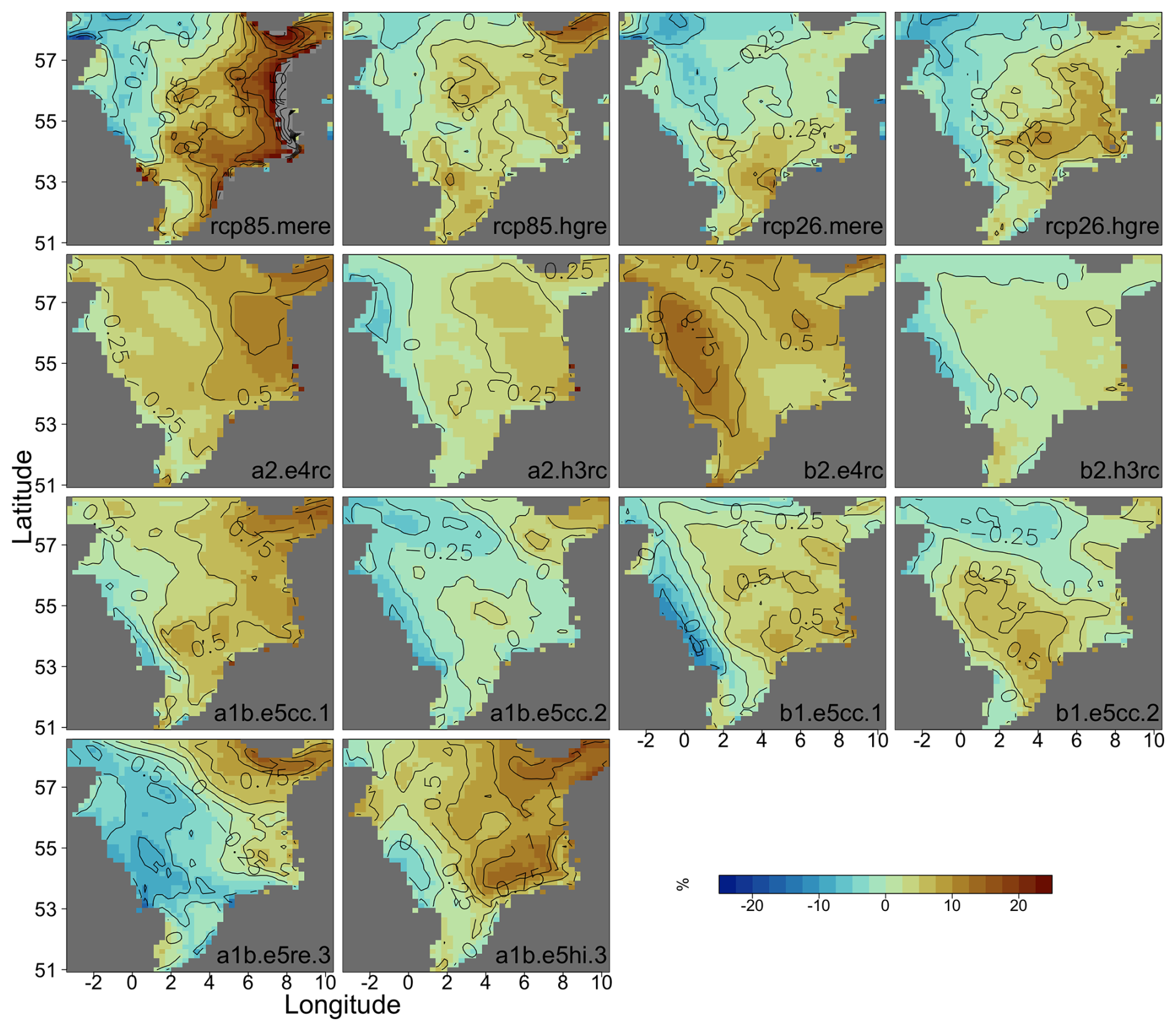
Figure A1 The individual climate change signals for the period 2071–2100 compared to the reference period 1961–1990 in the North Sea of the maximum SWH are shown for the 14 future climate projections (the abbreviations in the graphs represent the respective projections, as listed in Table 1). Colours indicate the relative change and contour lines indicate the absolute change.

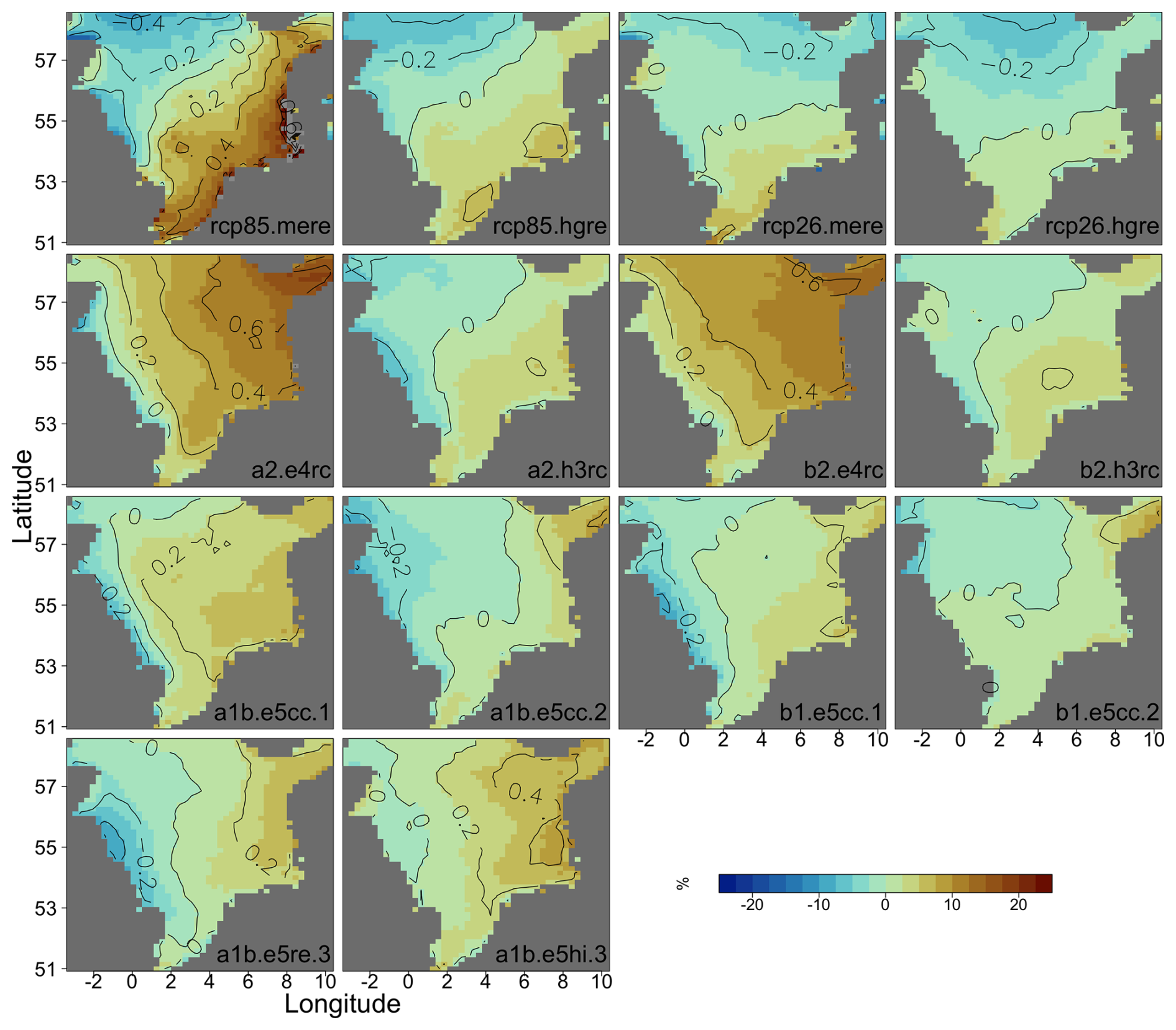
Figure A2 As Fig. A1 but for the 99th percentile SWH.

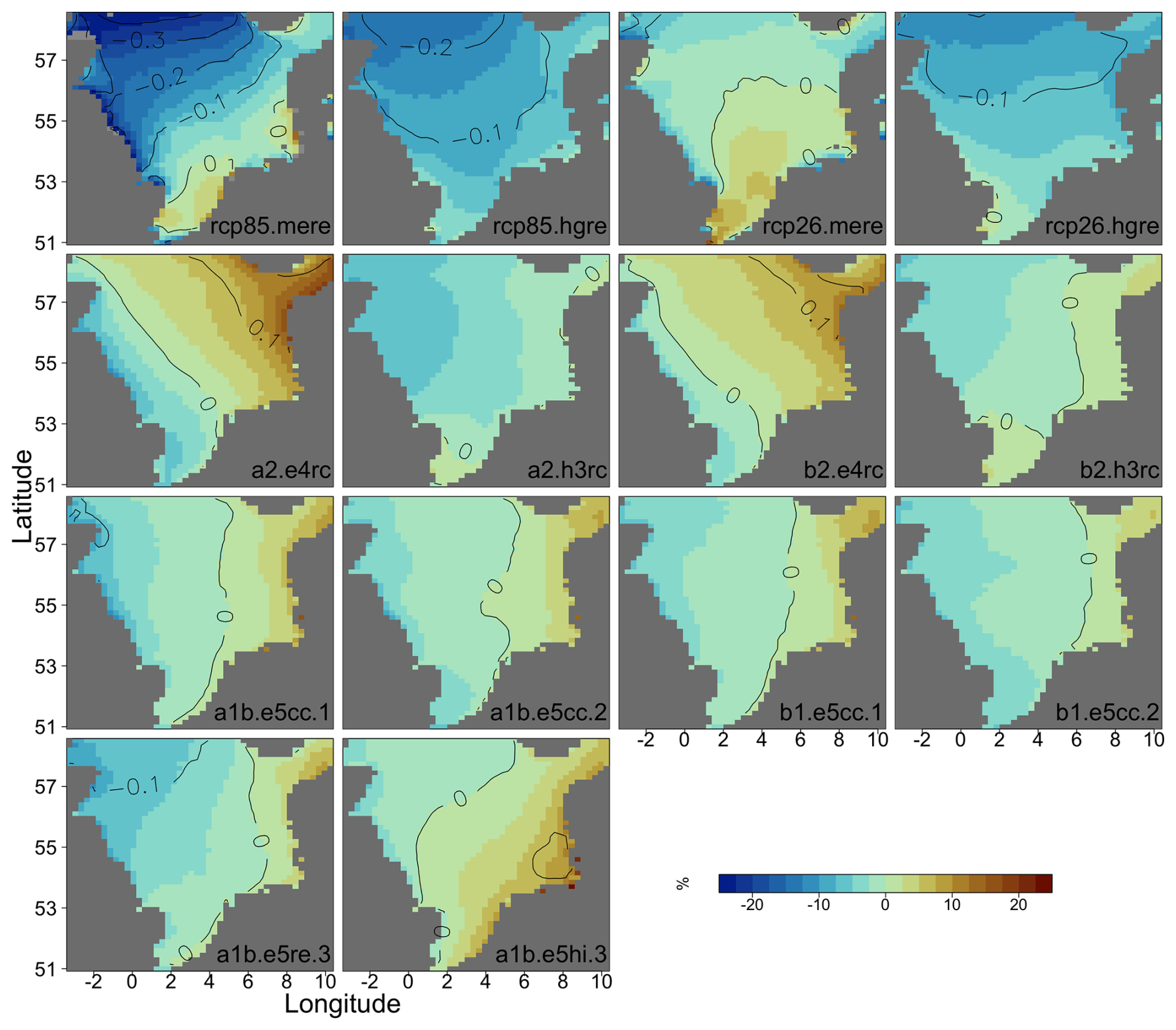
Figure A3 As Fig. A1 but for the median SWH.

A2 Baltic Sea

The climate change signals of the maximum SWH (Fig. A4), 99th percentile SWH (Fig. A5) and median SWH (Fig. A6) for individual simulations between the reference period 1961–1990 and the future period 2071–2100 are presented here.

When comparing the 30-year intervals 2071–2100 and 1961–1990, the maximum change in SWH is 15 %–20 % of the reference value. This change occurs in the south-eastern parts (up to 1 m), the northern parts and the Gulfs of Finland and Riga, depending on the projection (reaching approximately 0.5 m). For some projections, a local decrease of up to −10 % or −20 % occurs (0.25 to 0.5 m). The RCP26.mere projection shows larger areas with negative changes in the northern and south-western Baltic Sea.

The 99th percentile SWH show an increase in most regions at the end of the 21th century compared to the reference period, which can be up to 15 %–20 % (approximately 0.6 m) in the southern Baltic Sea in the RCP85.mere projection. The RCP26.mere and RCP26.hgre projections show the smallest increases, of around 0 %–5 % (about 0.1 m), and decreases of up to 5 % (about 0.1 m), mainly in the northern parts of the Baltic Sea.

The CMIP3 projections generally display a stronger increase in the Baltic Sea than the CMIP5 projections for the median. The strongest increase, exceeding 10 % (around 0.06 to 0.08 m), occurs in the northern parts of the A1B.e5cc.1 projection. The CMIP5 projections show an increase in most northern regions, but three projections show a small decrease of up to 5 % (around 0.02 m) in central Baltic Sea.

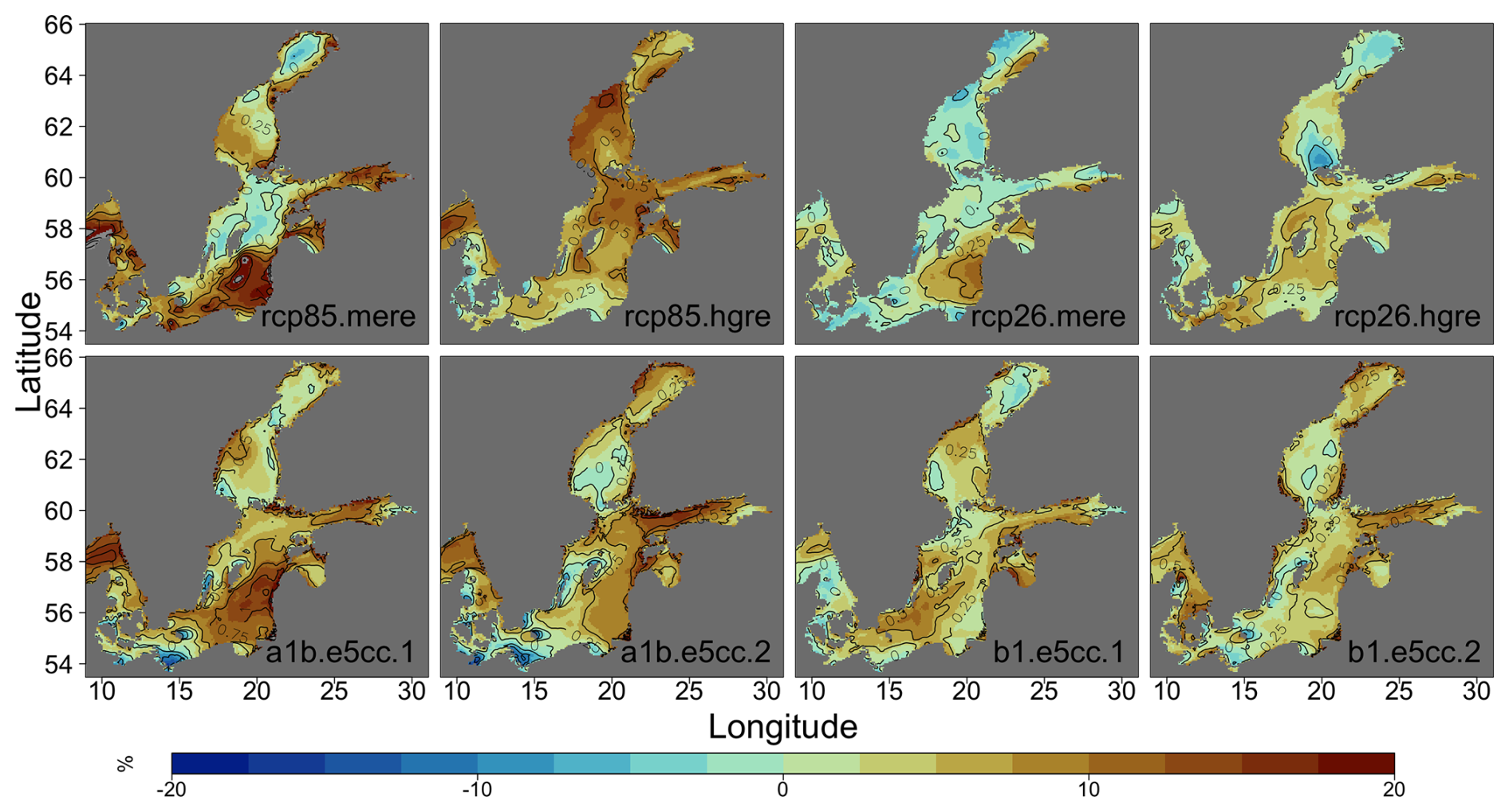
Figure A4 The individual climate change signals for the period 2071–2100 compared to the reference period 1961–1990 in the Baltic Sea of the maximum SWH are shown for the 8 future climate projections (the abbreviations in the graphs represent the respective projections, as listed in Table 1). Colours indicate the relative change and contour lines indicate the absolute change.

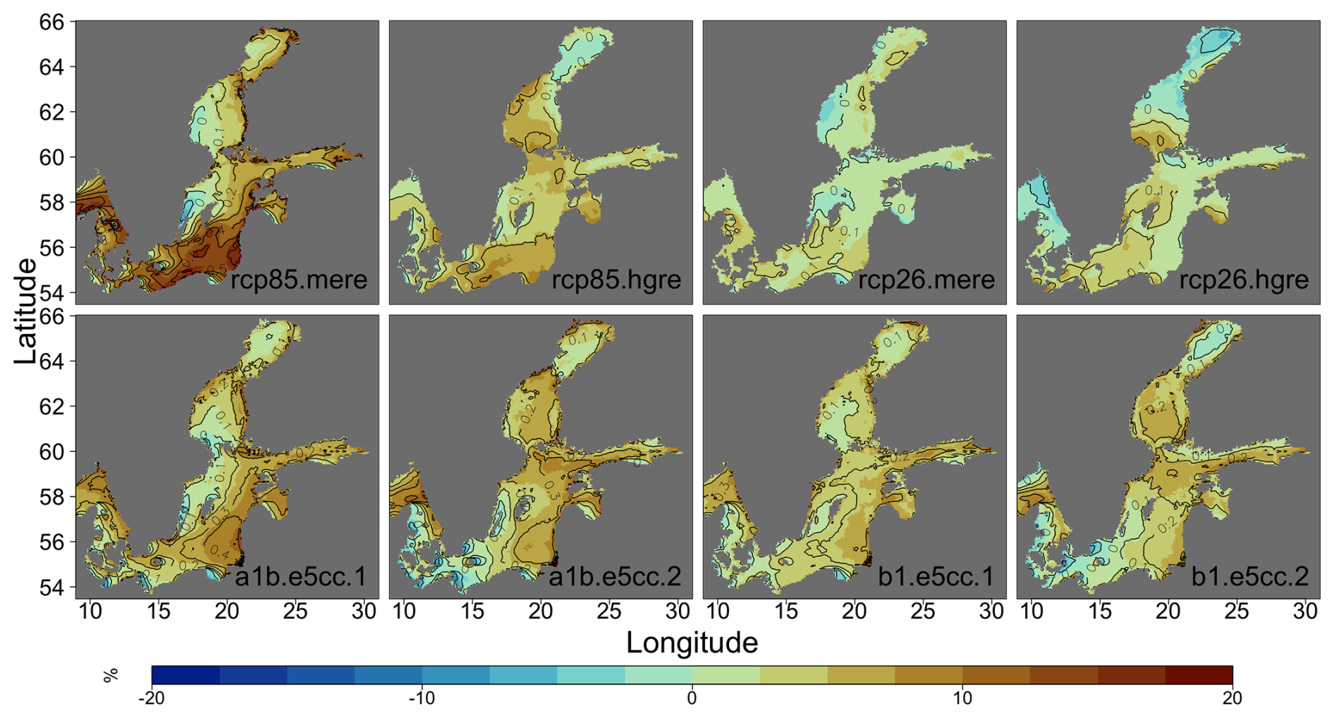
Figure A5 As Fig. A4 but for the 99th percentile SWH.

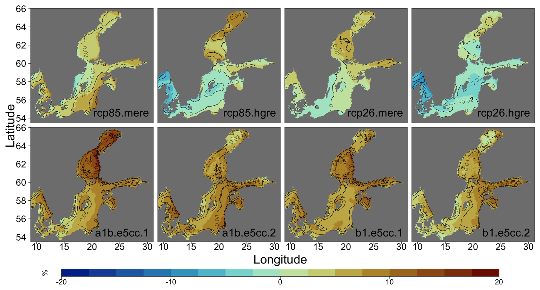
Figure A6 As Fig. A4 but for the median SWH.

Appendix B: Distribution comparison of the significant wave height in the historical period

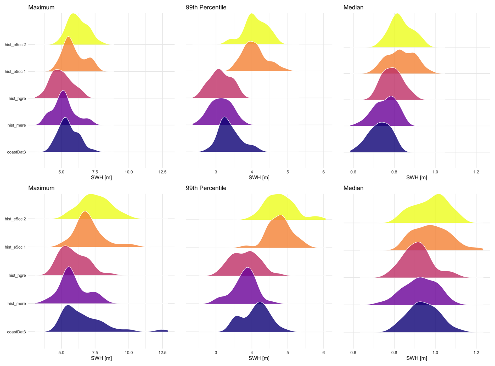
To test the model's ability to reproduce the SWH in the reference period, a distributional comparison between the model members and a reference dataset was done at two locations in the North Sea GBI and TYN (Fig. B1), and at two locations in the Baltic Sea, ARB and CBP (Fig. B2). As reference dataset the regional wave hindcast coastDat3 (Groll, 2024) was used. However, as the historical parts of the climate projections only incorporate greenhouse gas concentrations and no actual weather information, a direct comparison of the time series is not meaningful. Instead, the comparison is structured across three statistical metrics: Maximum, 99th percentile and median SWH, are displayed as density distributions for each location. The overall distributions of the climate models for the maximum, 99th percentile and median SWH at the location GBI (Fig. B1, upper panels) in the south-eastern North Sea show very similar distributions with minimal deviation from the hindcast distribution. This demonstrates that the wave conditions are reliably represented. At the location TYN in the western North Sea (see Fig. B1, lower panels), the distribution ranges for the climate models are generally broader than the range for coastDat3, with several models showing notably flatter distributions, particularly hist_e5hi.3. While most climate models show a comparable distribution with an acceptable difference to the reference, model member hist_e5hi.3 shows substantially higher 99th percentile and median values, representing a considerable difference in these wave conditions. As fewer climate simulations are available for the Baltic, only four historical simulations are compared with the hindcast coastDat3. At the location ARB in the western Baltic Sea (see Fig. B2, upper panels), the distributions of the two CMIP5 models (hg.re and me.re) are within the range of the hindcast, while the distributions of the other two models are slightly shifted towards higher values. Nevertheless, all climate model simulations provide a generally reliable representation of the wave conditions. Finally, the maximum distributions at location CBP in the central Baltic (see Fig. B2, lower panels) are notably broader than those at ARB. All four climate model distributions fall well within the range of the hindcast distribution for the whole simulated domain. While the CMIP5 climate models demonstrate good overall agreement with the 99th percentile hindcast distribution, the other two climate model distributions are slightly broader and shifted towards higher values. All climate models show good agreement with the relatively narrow, well-defined median distributions. Although differences are observed between the absolute values from the climate model simulations and the hindcast data, particularly at location TYN, and the notable inter-model variability underscores the challenges of reproducing absolute wave climate characteristics using climate models. The overall conclusion is that the distributions from the climate models are in good agreement with the reference hindcast. However, due to the differences in absolute values, the main analysis focuses on the relative changes that occur between different time periods, rather than the absolute values themselves.

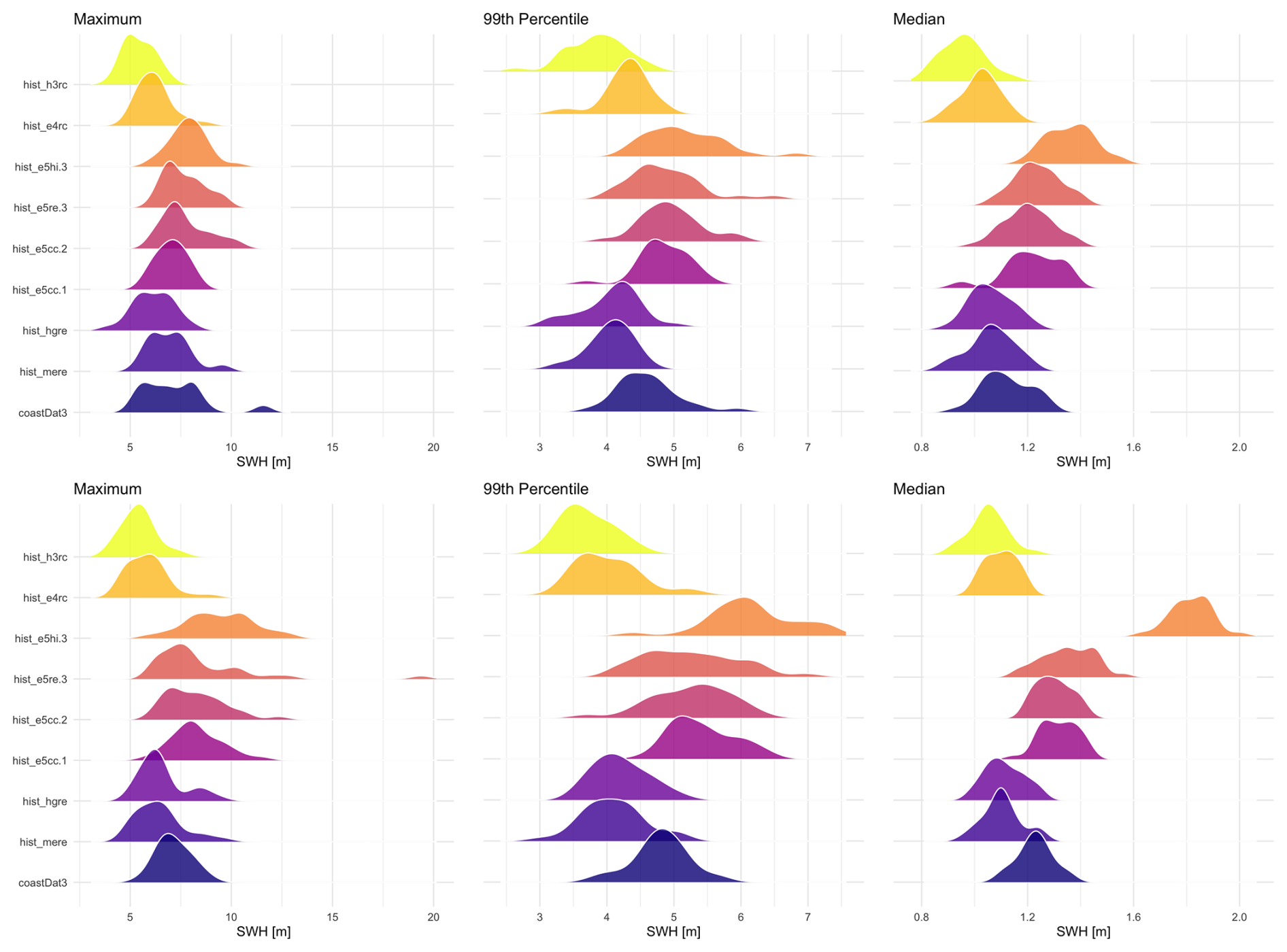
Figure B1 The density distribution of maximum, 99th percentile and median SWH for the historical simulation (hist_) and the hindcast simulation (coastDat3) for two locations in the North Sea (GBI in the upper panels and TYN in the lower panels). The abbreviation after hist_ indicates the respective ensemble member, as shown in Table 1.

Figure B2 As Fig. B1, but for two locations in the Baltic Sea (ARB in the upper panels and CBP in the lower panels).