Current status of ocean observation, ensemble reanalysis and CMIP6 models in describing Antarctic Bottom Water

Antarctic Bottom Water (AABW), a key component of the global meridional overturning circulation, forms in key regions around the Antarctic margin. This study applies a classification combining neutral density, subtype-specific salinity ranges, and prescribed geographical sectors to identify Weddell–Prydz Bottom Water (WPBW), Ross Sea Bottom Water (RSBW), and Adélie Land Bottom Water (ALBW). Using the World Ocean Atlas 2023 (WOA23) as an “observed” climatological reference, we evaluate to what extent current ocean ensemble reanalysis and CMIP6 climate models can reproduce observed AABW subtype-specific spatial distributions and thermohaline characteristics in deep ocean layers. The ensemble reanalysis generally reproduces spatial distributions and thermohaline properties of the three AABW subtypes. Most CMIP6 models show poor identification of the three subtypes, identifying only a small portion or no subtype distributions at all. Among CMIP6 models, CESM1-CAM5-SE-LR reasonably reproduces the general distribution of the three subtypes. The AABW identification does not improve with increasing model horizontal resolution. The poor identification can be improved to some extent after a regional thermohaline mean-state correction is applied, suggesting that some deficiencies might arise from models' systematic thermohaline offsets, whereas others reflect models' structural spatial biases. Our assessment indicates that modeled regional deficiencies may be obscured when AABW is treated as a single water mass.

1 Introduction

Antarctic Bottom Water (AABW) is the coldest and densest water mass in the global ocean. AABW is primarily sourced from coastal polynyas and extends across the world's oceans, constituting approximately 30 %–40 % of the global ocean volume (Johnson et al., 2008). As the principal driver of the lower limb of the global meridional overturning circulation (Orsi et al., 1999), the formation and transport of AABW significantly influence the vertical redistribution of heat (Purkey and Johnson, 2010) and the ocean's capacity for long-term carbon sequestration (Burke and Robinson, 2012; Marinov et al., 2006; Zhang et al., 2023). Therefore, understanding the spatial distribution and variability of AABW is crucial for assessing oceanic heat budgets and biogeochemical cycles in the context of global warming. However, in situ observations of AABW remain limited due to the extensive sea ice cover and extreme climatic conditions over the Antarctic continental shelf and slope regions. Furthermore, because AABW predominantly resides at depths exceeding 2000 m, its characterization using satellites or conventional buoys remains very challenging (Silvano et al., 2023).

Observational data form the foundation for AABW research. Repeat hydrographic sections remain the primary observational constraint on AABW properties (Purkey and Johnson, 2013; Silvano et al., 2023) and provide an important observational basis for climatological AABW (Locarnini et al., 2024; Reagan et al., 2024). Although these sections provide high-quality full-depth measurements along key transects, their spatial coverage remains sparse and their temporal sampling is discontinuous (Silvano et al., 2023). Building on these observations, WOA23 integrates a broad range of historical temperature and salinity profile observations with rigorous quality control (Locarnini et al., 2024; Reagan et al., 2024). Although it attenuates small-scale, regional, and transient signals due to smoothing and averaging, WOA23 is well suited for representing the large-scale, long-term averaged climatic state of AABW. Recently, understanding the variability and trend of AABW has become increasingly important, especially in a warming climate. In this context, ocean reanalysis products and climate models provide valuable datasets.

A few ocean reanalysis products have been used to study AABW. Among them, ECCO2 can generally reproduce the upper limit of AABW (defined by a density threshold γⁿ ≥ 28.27 kg m⁻³, Azaneu et al., 2014), but the post-2004 ECCO2 exhibits unrealistic open-ocean polynyas and deep convection in the Weddell Sea region, failing to capture the Weddell Sea Bottom Water (Azaneu et al., 2014). The German contribution to the Estimating the Circulation and Climate of the Ocean project (GECCO2; Köhl, 2015) shows a substantial fresh bias throughout the water column, whereas the Global Ocean Reanalyses and Simulations Stream 2 version 4 (GLORYS2V4; Lellouche et al., 2013) and the Met Office Global Seasonal forecasting system version 5 with the Global Ocean 5.0 configuration (GloSea5-GO5; MacLachlan et al., 2015; Megann et al., 2014) are generally saltier in certain layers. Taken together, the multi-reanalysis ensemble mean provides better agreement with the observations (Uotila et al., 2019). In addition, global climate models (i.e., the models participating in the Coupled Model Intercomparison Project Phase 6, CMIP6) are increasingly used to study AABW. However, only a few CMIP6 models can represent the shelf overflow processes, with most models relying instead on open-ocean deep convection, particularly in the Weddell and Ross Seas. As a result, the multi-model mean AABW is generally warmer, fresher, and lighter than the observations (Heuzé, 2021). These issues highlight the necessity of further evaluating the ability of reanalysis and climate model datasets to represent AABW formed in different regions.

The Weddell Sea, Ross Sea, Adélie Coast, and Prydz Bay are widely recognized as the four primary source regions of AABW (Gordon et al., 1993; Williams et al., 2008; Ohshima et al., 2013; Silvano et al., 2023). However, significant differences exist in physical processes governing AABW formation in these regions. These include variations in the intensity and direction of prevailing wind fields, sea-ice production rates, basal ice-shelf melt rates, and oceanic dynamical processes (e.g., overflows and mixing) (Pardo et al., 2012; Schmidt et al., 2023; Silvano et al., 2018, 2023; Han et al., 2024, 2025). Such differences lead to distinct regional characteristics in the initial temperature and salinity signatures of the source water, and consequently to marked differences in AABW properties in the deep ocean layer (Orsi et al., 1999; Silvano et al., 2023). To date, large-scale studies conventionally treat AABW as a broadly uniform water mass. Although this provides a useful framework for circumpolar analysis, it cannot fully capture distinct thermohaline properties that exist in AABW formed in different regions (Rintoul, 2018; Zhang et al., 2023). A source-region perspective on AABW is important because abyssal warming varies spatially across ocean basins (Purkey and Johnson, 2010), the bottom-water transport and ventilation undergo substantial regional changes (Gunn et al., 2023), and dense shelf water export transports anthropogenic carbon from the Antarctic shelf into the deep ocean (Zhang et al., 2023).

The present study applies a classification combining neutral density, subtype-specific practical-salinity ranges, and prescribed geographical sectors to identify Weddell–Prydz Bottom Water (WPBW), Ross Sea Bottom Water (RSBW), and Adélie Land Bottom Water (ALBW). Taking WOA23 as a benchmark, we examine spatial distributions and thermohaline properties of the three AABW subtypes. We then systematically evaluate whether the ensemble reanalysis and CMIP6 climate models can reproduce these subtype-specific thermohaline characteristics and spatial distributions. Our evaluation is intended to provide the current status of ocean observation, ensemble reanalysis, and CMIP6 models in describing AABW originating from different source regions, facilitating future investigations into distinctive characteristics and variability of AABW.

2 Data and Methods

2.1 Data

2.1.1 Observational data

This study utilizes full-depth ocean temperature and salinity climatological objective analysis fields from WOA23 (Reagan et al., 2024; Locarnini et al., 2024), covering the period 1991–2020. The data are provided on a 0.25° latitude–longitude grid with 102 vertical levels. WOA23 is a global ocean climatology product developed and distributed by the National Centers for Environmental Information of the National Oceanic and Atmospheric Administration. The dataset integrates measurements from multiple observational platforms and has undergone rigorous quality control procedures. These include removal of duplicate records, range and gradient checks, statistical significance testing based on 3–5 standard deviation thresholds, hydrostatic stability verification, and manual flagging of suspicious values. In addition, uncorrected real-time Argo salinity data have been excluded. To address the warm bias associated with Expendable Bathythermograph and Mechanical Bathythermograph measurements relative to bottle/CTD temperature data (Gouretski and Koltermann, 2007), the bias-correction scheme described by Levitus et al. (2009) is applied. For salinity, the initial quality-controlled profiles are interpolated to standard depth levels using the Reiniger–Ross method, followed by the objective analysis via the Barnes scheme. To mitigate spurious vertical density instabilities arising from inconsistencies between temperature and salinity profiles, often due to the greater abundance of temperature observations, a joint stabilization algorithm is applied (Jackett and McDougall, 1995). This procedure ensures that the final temperature and salinity fields yield a hydrostatically stable water column.

2.1.2 Reanalysis data

This study utilizes the ensemble mean of seawater potential temperature and salinity from 1993 to 2022, derived from the Global Ocean Ensemble Physics Reanalysis (Product ID: GLOBAL_MULTIYEAR_PHY_ENS_001_031; Copernicus Marine Service, 2023). This dataset integrates outputs from three independent ocean reanalysis systems: GLORYS2V4 (Mercator Ocean; Lellouche et al., 2013), ORAS5 (ECMWF; Zuo et al., 2019), and C-GLORSv5 (CMCC; Storto and Masina, 2016). It delivers monthly averaged variables, including temperature, salinity, current velocity, and sea surface height, from 1993 onward, at a horizontal resolution of 0.25° and with 75 vertical layers. The production system is based on the Nucleus for European Modelling of the Ocean (NEMO) model and the ORCA025 global tripolar ocean grid with a nominal horizontal resolution of 0.25°, and is forced by ERA-Interim and ERA5 atmospheric fields. Multi-source observational data are assimilated, encompassing sea level anomalies, sea surface temperature, sea ice concentration, and in situ temperature/salinity profiles. The ensemble is constructed via post-processing of the three reanalysis members, which differ in their model versions, surface forcing treatments, and data assimilation schemes. This diversity enhances the robustness and stability of the ensemble estimates.

2.1.3 Model outputs

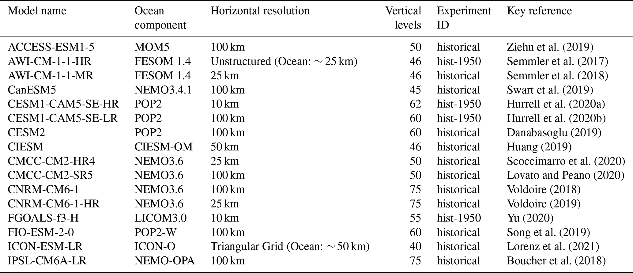
This study utilizes data from 16 CMIP6 models, selected based on the availability of either the “historical” experiment or the “hist-1950” experiment and on the condition that monthly output for seawater salinity and potential temperature was accessible as of the data retrieval cutoff date. All selected models provide output on standard z-coordinates. Only the AWI-CM-1-1-HR dataset has a shorter period (1993–2010) compared to the others (1993–2014). Details of each model are provided in Table 1.

Table 1 Information on the 16 CMIP6 models utilized in this study, including their ocean component, nominal horizontal resolution, number of vertical levels, experiment ID and corresponding official references.

2.2 Methods

Antarctic Bottom Water is first identified using the classical neutral-density criterion γⁿ ≥ 28.27 kg m⁻³ (Orsi et al., 1999). This density-only distribution is used as a physical reference for assessing the additional effects of the practical salinity and geographical constraints. We know that for the cold waters in the Antarctic, the thermal expansion coefficient of seawater plays a relatively minor role, making salinity the primary factor for density. Then the salinity values of 34.650, 34.695, and 34.683 reported by Pardo et al. (2012) are used for the Weddell Sea Bottom Water, Ross Sea Bottom Water, and Adélie Land Bottom Water, respectively. Note that they represent source-water endmembers derived within an Optimum Multiparameter framework rather than the mean properties of fully mixed AABW in the ocean interior. In this study, these values are used only as central hydrographic reference values and are not used to calculate water-mass fractions or to quantitatively attribute an individual water mass to a unique formation source. For the classification adopted here, AABW satisfying the adopted neutral-density and salinity criteria within the Weddell–Prydz sector is referred to as Weddell–Prydz Bottom Water (WPBW). This sectoral hydrographic category is used to facilitate basin-scale comparison and does not imply an OMP-type decomposition or a quantitative merging of distinct source-water contributions. We perform the sensitivity analysis to determine our final classification, which can be found in Sect. 2.3.

The primary analysis is performed at the 4000 m depth level and in the near-bottom layer. The 4000 m level is commonly used to quantify changes in the abyssal ocean (Purkey and Johnson, 2010; Li et al., 2023), and all datasets are vertically interpolated to this depth for comparison. For the near-bottom analysis, the deepest valid level in each dataset is selected, provided that the two immediately overlying levels also contain valid data, thereby reducing the influence of isolated or spurious values. Because the exact depth of the selected near-bottom level varies among datasets, slight differences in the sampled depths may remain. To provide additional information on the vertical persistence of the identified AABW subtypes, practical salinity and subtype diagnostics are also conducted at 3500 and 4500 m, which are presented in the Supplement. These supplementary diagnostics are used to assess whether the identified bottom-water characteristics remain spatially coherent across multiple abyssal depth levels and to distinguish limited vertical extension from more general biases in the simulated deep-ocean thermohaline structure and regional distribution.

2.3 Sensitivity analysis

Here we evaluate the robustness of our AABW subtype classification. We first identified the spatial footprint of AABW using only the classical neutral-density criterion γⁿ ≥ 28.27 kg m⁻³ (Table 2). Based on WOA23, waters satisfying this criterion are mainly distributed from the eastern Ross Sea to the Bellingshausen Sea, from the central Weddell Sea toward the Indian Ocean sector, and along the East Antarctic continental margin between approximately 75 and 150° E at both the 4000 m and near-bottom layers (Fig. S1 in the Supplement).

Table 2 Hydrographic and geographical criteria used to identify the AABW subtypes in this study. The practical salinity endmember values reported by Pardo et al. (2012) are used only as central hydrographic references. The identified categories represent hydrographic AABW subtypes with properties characteristic of the respective source regions rather than unmixed endmembers or quantitative source-water fractions.

We then assessed the sensitivity of the subtype classification to the practical-salinity ranges applied around the central hydrographic reference values reported by Pardo et al. (2012). Four progressively widened ranges were tested, including $\mathrm{\Delta }S=\pm$0.01, ±0.02, ±0.03, and ±0.04. For each test, the neutral-density threshold was retained, and the spatial distributions and identified areas of WPBW, RSBW, and ALBW were calculated at the 4000 m and near-bottom layers (Fig. 1). Under the narrowest range of $\mathrm{\Delta }S=\pm$0.01, the identified subtype distributions are relatively restricted. At 4000 m, the identified areas of WPBW, RSBW, and ALBW are 4.96, 2.53, and 2.03 × 10⁶ km², respectively, compared with 8.36, 2.92, and 3.25 × 10⁶ km² when only the neutral-density criterion is applied (Table 3).

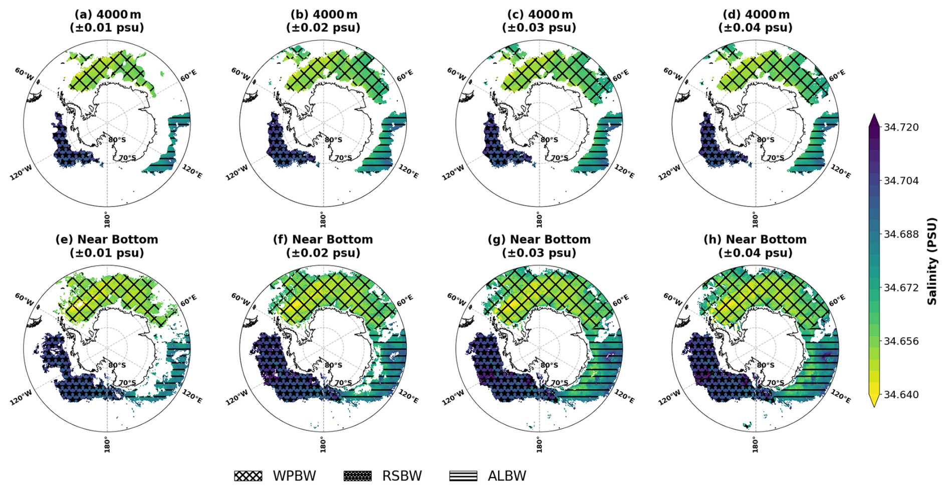
Figure 1 Spatial distributions of the identified Antarctic Bottom Water (AABW) subtypes under different practical-salinity ranges (ΔS). The top row (a–d) and bottom row (e–h) represent the 4000 m depth layer and the near-bottom layer, respectively. Columns from left to right show classifications based on applied ΔS values of ±0.01, ±0.02, ±0.03, and ±0.04 around the central salinity values (WPBW: 34.650; RSBW: 34.695; ALBW: 34.683). All classifications are additionally constrained by the neutral-density threshold (γⁿ ≥ 28.27 kg m⁻³). The respective AABW subtypes are distinguished by distinct hatching patterns, as detailed in the figure legend. Background shading represents practical salinity.

Table 3 Calculated areas (10⁶ km²) of the three AABW subtypes under different practical-salinity ranges (ΔS) at the 4000 m layer and the near-bottom layer. These thresholds are defined around the central salinity values (WPBW: 34.650; RSBW: 34.695; ALBW: 34.683).

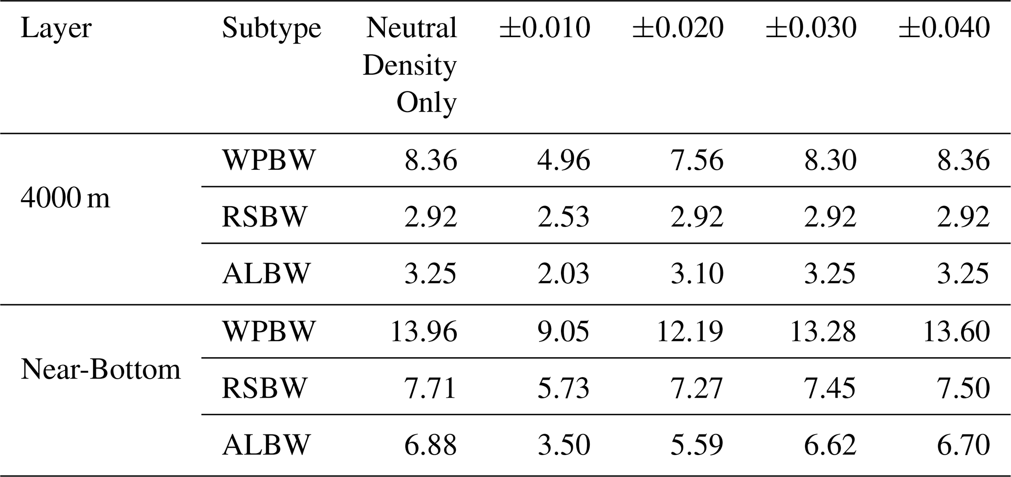
When the practical-salinity range is widened to $\mathrm{\Delta }S=\pm$0.02, the three AABW subtypes within their respective prescribed longitudinal sectors exhibit spatial distributions similar to those based on the neutral-density-only criterion at both the 4000 m and near-bottom layers (Fig. 1). At 4000 m, the corresponding identified areas increase to 7.56, 2.92, and 3.10 × 10⁶ km² for WPBW, RSBW, and ALBW, respectively. Further widening to $\mathrm{\Delta }S=\pm$0.03 or ±0.04 does not lead to an abrupt spatial reorganization; instead, it mainly produces a gradual expansion of the peripheral boundaries, and the identified areas slowly converge toward those obtained using the neutral-density-only criterion (Table 3). Similar behavior is found at the near-bottom layer.

Given that a practical-salinity range wider than ±0.02 may include diluted peripheral waters and parts of the overlying Circumpolar Deep Water, $\mathrm{\Delta }S=\pm$0.02 is adopted in the final classification. This range provides a reasonable balance between identifying the principal bottom-water bodies and avoiding the excessive inclusion of peripheral waters and overlying Circumpolar Deep Water. It also allows moderate modification of the source-water properties through mixing and downstream spreading, rather than requiring the salinity of individual grid cells to exactly match the source-water endmember values.

Temperature is already incorporated into the calculation of neutral density, and therefore contributes to the initial identification of AABW. To determine whether potential temperature could provide an additional independent constraint for distinguishing the three AABW subtypes, we tested progressively widened potential-temperature ranges of $\mathrm{\Delta }T=\pm$0.10, ±0.20, ±0.30, ±0.40, and ±0.50 °C around the corresponding central values reported by Pardo et al. (2012). The neutral-density criterion was retained in all tests and the spatial distributions and identified areas of WPBW, RSBW, and ALBW were calculated at the 4000 m and near-bottom layers (Fig. S2). Under the narrowest potential-temperature range of $\mathrm{\Delta }T=\pm$0.10 °C, the identified subtype areas are small and spatially fragmented. At 4000 m, no WPBW is identified, and the identified areas of RSBW and ALBW are only 0.15 and 0.41 × 10⁶ km², respectively. When the range is widened to $\mathrm{\Delta }T=\pm$0.30 °C, the identified areas of WPBW, RSBW, and ALBW increase substantially to 2.74, 1.31, and 2.03 × 10⁶ km², respectively. At $\mathrm{\Delta }T=\pm$0.50 °C, the corresponding areas increase further to 6.23, 2.92, and 3.11 × 10⁶ km². A similar expansion is found at the near-bottom layer, where the identified areas increase from 2.19, 0.63, and 2.23 × 10⁶ km² at $\mathrm{\Delta }T=\pm$0.10 °C to 10.47, 7.42, and 6.35 × 10⁶ km² at $\mathrm{\Delta }T=\pm$0.50 °C for WPBW, RSBW, and ALBW, respectively (Fig. S2 and Table S1).

Although the increase in the identified area is an expected consequence of widening the classification range, the potential-temperature sensitivity analysis does not exhibit a clear stage at which the principal spatial patterns become relatively stable. By contrast, once the salinity range reaches $\mathrm{\Delta }S=\pm$0.02, the principal distributions of the three AABW subtypes remain broadly consistent, and further widening mainly produces a gradual expansion of their boundaries. A fixed potential-temperature range therefore provides a less stable standalone constraint for the subtype classification than the adopted practical-salinity criterion.

Based on the spatial distribution of regionally sourced AABW, WPBW is confined to the sector between 60° W and 70° E, RSBW to the sector between 160 and 180° E and between 180 and 60° W, and ALBW to the sector between 70 and 160° E (Table 2). Thus, the final classification combines the classical neutral-density criterion, subtype-specific practical-salinity ranges of $\mathrm{\Delta }S=\pm$0.02, and the prescribed geographical sectors (Table 2). Potential temperature is not imposed as an additional independent classification threshold but is subsequently evaluated within the identified subtype regions as a diagnostic property for characterizing their thermohaline properties and assessing biases in the ensemble reanalysis and CMIP6 models.

3 Results

3.1 WOA23 observational data

At the 4000 m layer, the three identified AABW subtypes exhibit distinct spatial distributions and thermohaline characteristics (Fig. 2a and c). RSBW is characterized by relatively high potential temperature and practical salinity, and is predominantly distributed in the eastern Ross Sea, Amundsen Sea, and Bellingshausen Sea. In contrast, WPBW exhibits lower potential temperature and practical salinity, and is mainly found in the Weddell Sea. ALBW has intermediate thermohaline properties and a relatively fragmented spatial distribution, primarily occurring along the East Antarctic continental margin between approximately 75 and 150° E (Fig. 2a and c).

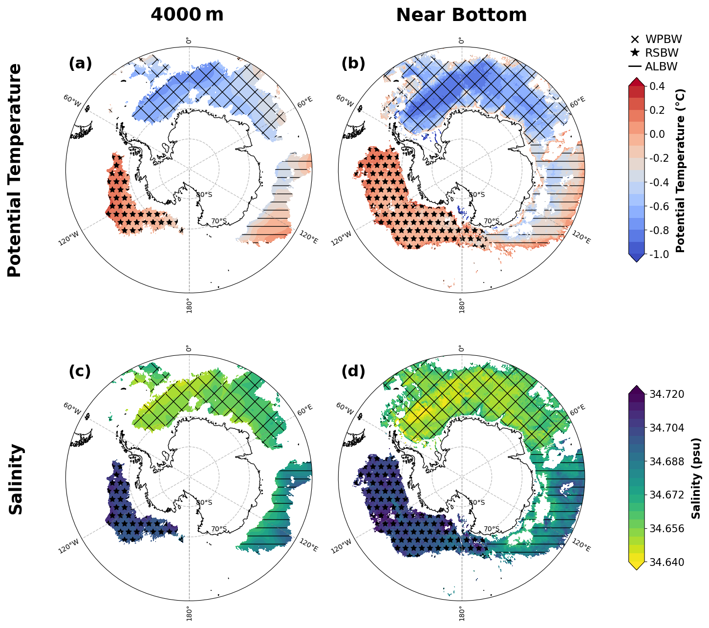
Figure 2 Spatial distributions of Antarctic Bottom Water (AABW) subtypes in the 1991–2020 WOA23 climatology. Panels (a) and (b) show potential temperature at the 4000 m and near-bottom layers, respectively, while panels (c) and (d) show practical salinity at the corresponding depth levels. The AABW subtypes are identified using the neutral-density, practical-salinity, and geographical criteria described in Sect. 2.2 and 2.3. The respective AABW subtypes are distinguished by distinct hatching patterns, as detailed in the figure legend.

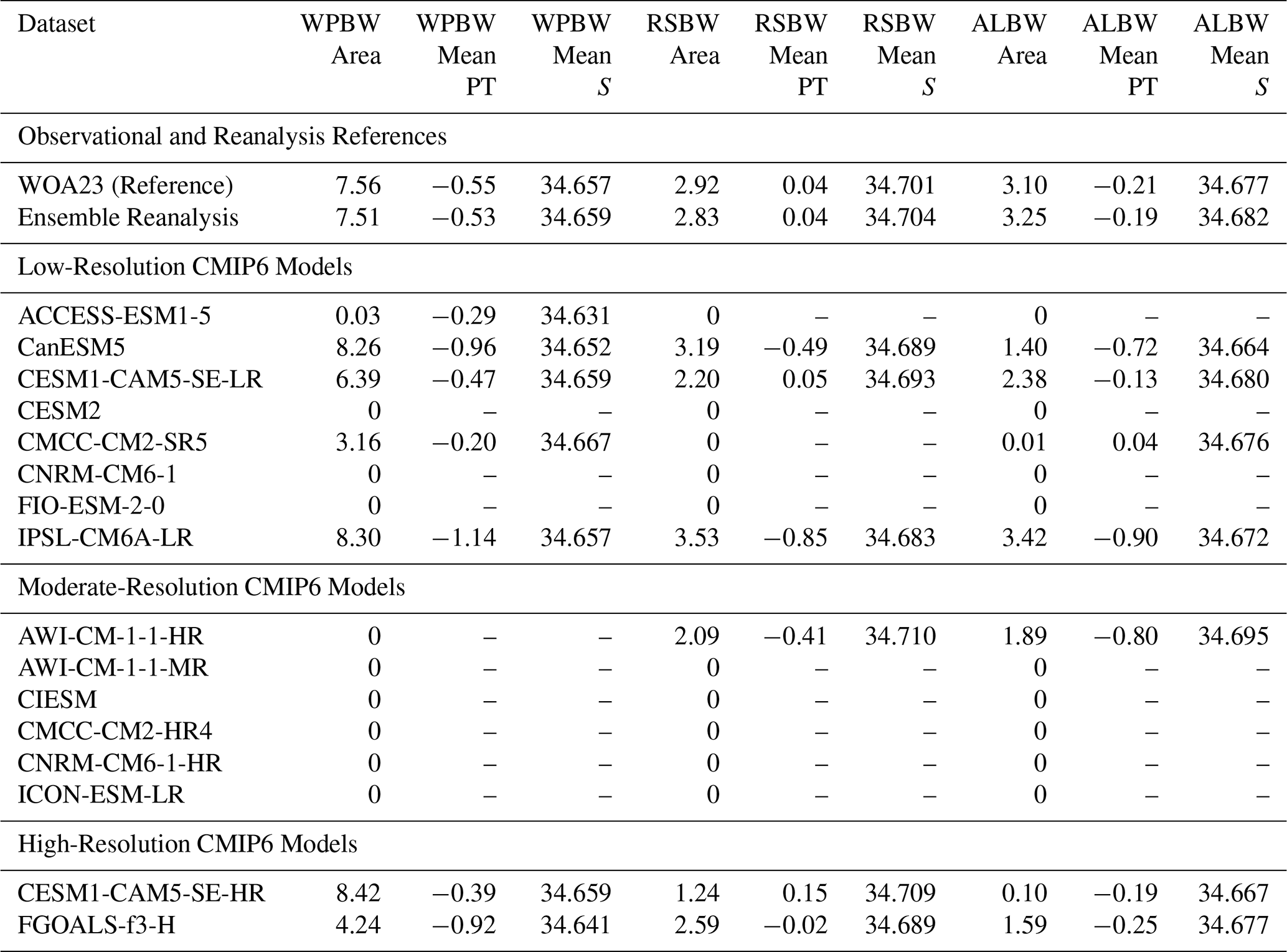
Quantitatively, the identified areas of WPBW, RSBW, and ALBW at 4000 m are 7.56, 2.92, and 3.10 × 10⁶ km², respectively (Table 4). Their corresponding mean potential temperatures are −0.55, 0.04, and −0.21 °C, and mean practical salinities are 34.657, 34.701, and 34.677, respectively. These results confirm that, among the three identified subtypes, RSBW is relatively warmer and more saline, WPBW is colder and fresher, and ALBW exhibits intermediate thermohaline properties.

Table 4 Quantitative metrics of the simulated Antarctic Bottom Water (AABW) subtypes at the 4000 m depth layer across the Southern Ocean (south of 50° S). The table details the spatial area (10⁶ km²), mean potential temperature (PT, °C), and mean practical salinity (S) for the Weddell–Prydz Bottom Water (WPBW), Ross Sea Bottom Water (RSBW), and Adélie Land Bottom Water (ALBW). Metrics are evaluated for the WOA23 climatological reference, the Ensemble Reanalysis, and 16 CMIP6 models. AABW subtype properties are averaged only over grid cells in each dataset that satisfy the prescribed density and salinity thresholds. A value of 0 in the area column indicates that no grid cells satisfy the prescribed criteria for the corresponding subtype. In such cases, the mean potential temperature and practical salinity cannot be calculated and are therefore denoted by dashes.

At the near-bottom layer, the overall distribution of AABW is consistent with previous studies (Orsi et al., 1999; Purkey et al., 2018), with RSBW exhibiting relatively high potential temperature and practical salinity, and WPBW showing lower values. Compared with the 4000 m layer, all three AABW subtypes occupy larger areas near the seafloor (Fig. 2b and d; Table S2). The identified areas of WPBW, RSBW, and ALBW increase to 12.19, 7.27, and 5.59 × 10⁶ km², respectively. Their mean potential temperatures are −0.62, −0.04, and −0.26 °C, and mean practical salinities are 34.654, 34.700, and 34.678, respectively.

The larger near-bottom extent is particularly evident for RSBW, which extends farther northward into the Bellingshausen Sea and occupies a broader zonal area across the Ross Sea than at 4000 m (Fig. 2). WPBW also expands, including a pronounced northward extension near 30° E. ALBW occupies a broader and more spatially continuous area along the East Antarctic continental margin than at 4000 m. Despite these changes in spatial extent, the relative thermohaline ordering of the three subtypes remains consistent between the two depth levels.

3.2 Ensemble Reanalysis

At the 4000 m layer, the ensemble reanalysis data indicate that, consistent with WOA23 observations, RSBW exhibits relatively high potential temperature and practical salinity, while WPBW exhibits a cooler and fresher signature. The identified areas of WPBW, RSBW, and ALBW are 7.51, 2.83, and 3.25 × 10⁶ km², respectively, corresponding to differences of about −0.7 %, −3.1 %, and +4.8 % relative to WOA23 (Table 4). Their mean potential temperatures and practical salinities are also close to the corresponding WOA23 values. The spatial extent of RSBW in the reanalysis data is slightly smaller than that in WOA23, primarily in the western and central Amundsen Sea, while ALBW is slightly more extensive and spatially continuous between 75 and 150° E (Fig. 3a and c). In contrast, WPBW closely matches the spatial distribution in WOA23.

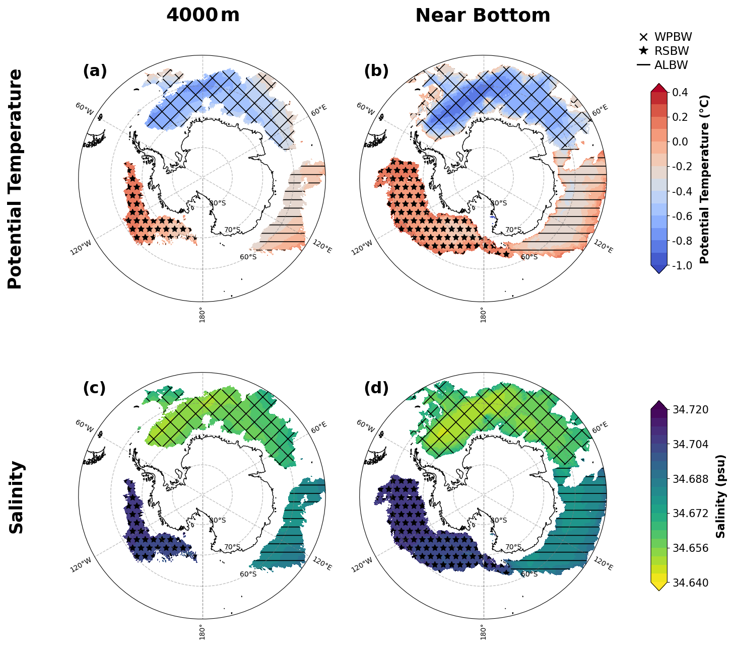
Figure 3 Spatial distributions of AABW subtypes in the 1993–2022 Ensemble Reanalysis dataset (GLOBAL_MULTIYEAR_PHY_ENS_001_031). Panels (a) and (b) show potential temperature at the 4000 m and near-bottom layers, respectively, while panels (c) and (d) show practical salinity at the corresponding depth levels. The respective AABW subtypes are distinguished by distinct hatching patterns, as detailed in the figure legend.

At the near-bottom layer, the reanalysis data further show that, consistent with the observation-based AABW distribution, RSBW is also characterized by relatively elevated potential temperature and practical salinity, whereas WPBW exhibits relatively lower temperature and salinity (Fig. 3b and d). The identified areas of WPBW, RSBW, and ALBW are 10.57, 6.33, and 6.01 × 10⁶ km², respectively (Table S2). Compared with WOA23, the ensemble reanalysis underestimates the near-bottom areas of WPBW and RSBW but slightly overestimates that of ALBW. The spatial extent of RSBW is somewhat reduced, primarily in the Ross-Amundsen sector. Similarly, the distribution of WPBW is more constrained relative to WOA23, particularly with reduced northward penetration. In contrast, ALBW covers a slightly broader and more spatially continuous area than in WOA23 within the longitudinal band of 75–150° E (Fig. 3b and d).

3.3 CMIP6 model simulations

As pointed out by Heuzé (2021), the performance of climate models in simulating AABW might be improved through two main approaches: increasing model resolution and improving parameterizations of complex physical processes. Ocean models with resolutions finer than 25 km can begin to describe the main structure of mesoscale eddies in open oceans (Chassignet and Xu, 2021; Hewitt et al., 2020). The representation of mesoscale eddies may influence the simulated thermohaline properties, export pathways, and spatial distribution of AABW. However, in some cases, coarser-resolution models may better represent certain physical process parameterizations, i.e., AABW formation and export are affected by the parameterization of unresolved overflow processes. Based on these considerations, CMIP6 models evaluated in this study are classified by the resolution of their ocean components into low-resolution (100 km), moderate-resolution (25–50 km), and high-resolution (10 km) groups. This classification is used to compare model behavior across different resolution ranges rather than to assume that higher-resolution models necessarily have better skill.

The original CMIP6 simulations are evaluated using complementary spatial and water-mass diagnostics. Taylor diagrams are first used to evaluate the large-scale spatial patterns of potential temperature and practical salinity relative to WOA23. The identified areas and mean thermohaline properties of WPBW, RSBW, and ALBW are then compared quantitatively at the 4000 m and near-bottom layers. Additional practical-salinity diagnostics at 3500 and 4500 m are used to examine whether the simulated bottom-water characteristics persist vertically.

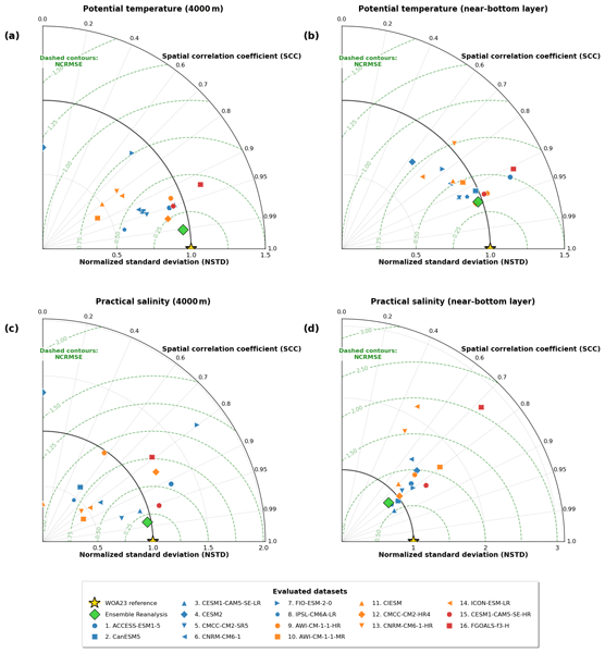
Figure 4 presents Taylor diagrams evaluating the potential-temperature and practical-salinity fields from the ensemble reanalysis and the 16 CMIP6 models relative to the WOA23 climatology over the Southern Ocean south of 50° S. The spatial correlation coefficient (SCC), calculated from spatial anomalies relative to the domain mean, measures the similarity between the simulated and WOA23 spatial patterns. The normalized standard deviation (NSTD) indicates whether the magnitude of simulated spatial variability is weaker or stronger than that in WOA23, whereas the normalized centered root-mean-square error (NCRMSE) summarizes the combined differences in spatial pattern and variability after removal of the spatial mean.

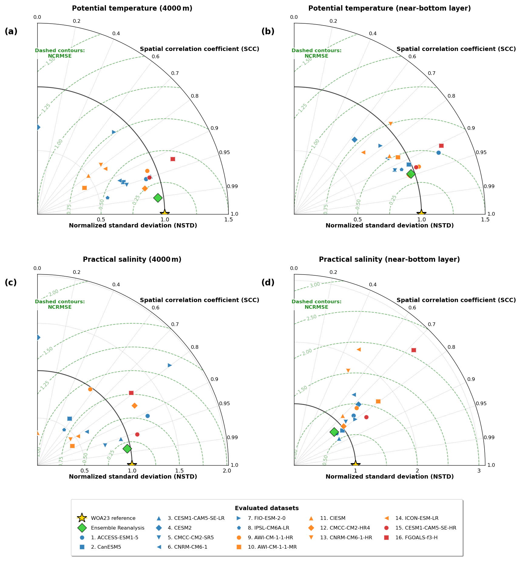
Figure 4 Taylor diagrams evaluating the ability of the simulations to reproduce the spatial distributions of thermohaline properties across the Southern Ocean south of 50° S. Panels (a) and (b) show potential temperature at 4000 m and in the near-bottom layer, respectively, whereas panels (c) and (d) show practical salinity at the corresponding depth levels. The thermohaline spatial fields from the Ensemble Reanalysis and 16 CMIP6 models are evaluated against the WOA23 climatological reference. The gold star at SCC = 1 and NSTD = 1 represents the WOA23 reference. In each diagram, the angular coordinate represents the spatial correlation coefficient (SCC), which measures the similarity between the simulated and reference spatial distributions, while the radial coordinate represents the normalized standard deviation (NSTD), which indicates the amplitude of simulated spatial variability relative to WOA23. The green dashed contours represent the normalized centered root-mean-square error (NCRMSE). The datasets are distinguished by color: the Ensemble Reanalysis is shown in green, low-resolution CMIP6 models in blue, moderate-resolution models in orange, and high-resolution models in red. Because the diagrams display only the non-negative-correlation quadrant, models with SCC ≤ 0 are plotted on the zero-correlation boundary. To prevent excessive stretching of the radial scale, data points with NSTD > 10 are not displayed.

Overall, the ensemble reanalysis is closest to the WOA23 reference, with high SCC values, NSTD values close to 1, and relatively small NCRMSE values in most diagnostics. This indicates that the reanalysis generally reproduces the large-scale abyssal thermohaline properties of WOA23.

Based on these three metrics, the CMIP6 models can be broadly divided into three categories. The first category includes models that retain recognizable regional thermohaline contrasts in most comparisons of potential temperature and practical salinity at 4000 m and in the near-bottom layer, indicating that their simulations do not deviate significantly from the WOA23 reference. These models generally have SCC values higher than about 0.75. Their NSTD values mostly fall within a moderate range around the WOA23 reference, about 0.7–1.4, and their NCRMSE values are generally located within the lower to intermediate error contours in the Taylor diagrams. ACCESS-ESM1-5, CESM1-CAM5-SE-LR, CMCC-CM2-SR5, CMCC-CM2-HR4, and CESM1-CAM5-SE-HR generally fall into this category. However, the subtype areas and mean thermohaline properties listed in Tables 4 and S2 also indicate that better Taylor-diagram performance does not necessarily mean that the AABW subtype extent and water-mass properties are accurately simulated.

The second category includes models that are unable to completely reproduce the abyssal thermohaline structure and whose performance is more sensitive to the variable, depth level, or amplitude of spatial variability. These models have positive SCC values for most diagnostics, but the spatial consistency is not maintained simultaneously across all diagnostics. Their NSTD values also deviate noticeably from 1 for one or more variable–depth combinations, indicating compressed or amplified spatial variability. Their NCRMSE values further suggest that these models have larger centered spatial-pattern errors than those in the first category. CanESM5, IPSL-CM6A-LR, AWI-CM-1-1-HR, AWI-CM-1-1-MR, CNRM-CM6-1, FIO-ESM-2-0, and FGOALS-f3-H can be assigned to this category.

The third category includes models that show clear structural deficiencies in at least one key diagnostic. CESM2 and CIESM are the most evident examples in the 4000 m practical-salinity field, where their SCC values are negative or close to zero. This indicates that their simulated salinity anomaly patterns are spatially opposite to those in WOA23, or have little correspondence with WOA23. CNRM-CM6-1-HR and ICON-ESM-LR can also be assigned to this category, because their near-bottom salinity diagnostics show little agreement with WOA23, with SCC values around 0.5 or lower and clearly distorted spatial variability. These results indicate that the model errors cannot be explained solely by spatially uniform warm/cold or saline/fresh biases, but also involve errors in the geographical placement, regional contrasts, or spatial gradients of the abyssal thermohaline fields. Because AABW subtype identification partly depends on characteristic practical-salinity signatures within prescribed geographical sectors, such structural errors tend to limit the ability of the models to reproduce the observed distributions and properties of WPBW, RSBW, and ALBW.

To improve the readability of the spatial comparison, Fig. 5 presents five representative models – CESM1-CAM5-SE-LR, IPSL-CM6A-LR, ACCESS-ESM1-5, CMCC-CM2-HR4, and CESM1-CAM5-SE-HR – while the complete spatial distributions for all 16 CMIP6 models are provided in Figs. S3 and S4. These five models span the low-, moderate-, and high-resolution groups and illustrate distinct original simulation characteristics.

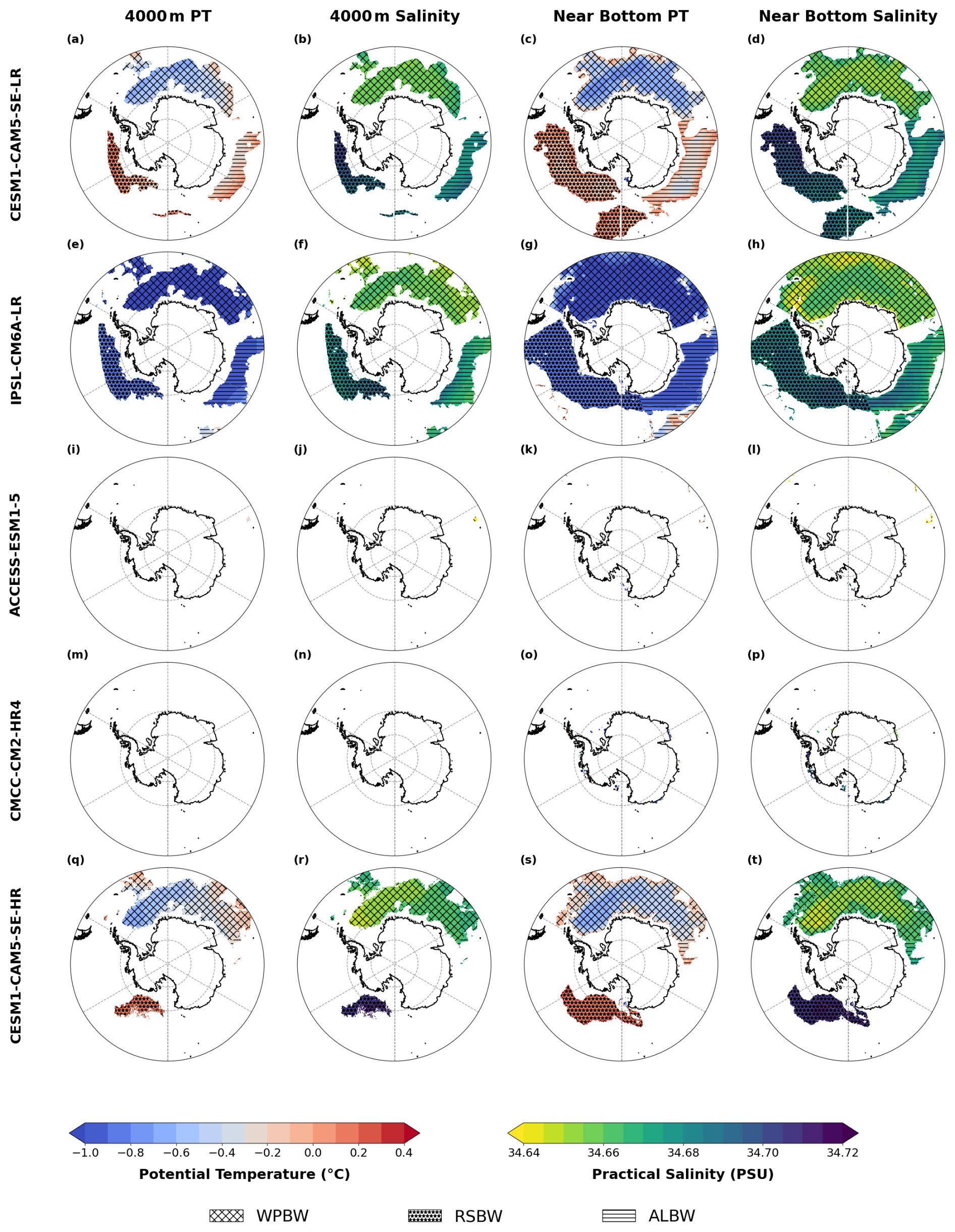
Figure 5 Spatial distributions of the original simulated potential temperature and practical salinity for Antarctic Bottom Water (AABW) subtypes across five representative CMIP6 models in the Southern Ocean (south of 50° S). The figure is organized into a 5 × 4 matrix. The rows represent the five representative CMIP6 models: CESM1-CAM5-SE-LR, IPSL-CM6A-LR, ACCESS-ESM1-5, CMCC-CM2-HR4, and CESM1-CAM5-SE-HR. The columns display the evaluated thermohaline properties: potential temperature at 4000 m, practical salinity at 4000 m, potential temperature at the near-bottom layer, and practical salinity at the near-bottom layer. Subpanels are labeled from (a) to (t). The respective AABW subtypes are distinguished by distinct hatching patterns, as detailed in the figure legend.

Among the three representative low-resolution models, the CESM1-CAM5-SE-LR model provides a reasonable representation of the general spatial patterns of the three AABW subtypes. At 4000 m, its identified WPBW, RSBW, and ALBW areas are 6.39, 2.20, and 2.38 × 10⁶ km², respectively, compared with 7.56, 2.92, and 3.10 × 10⁶ km² in WOA23. At the near-bottom layer, the corresponding areas are 10.07, 7.82, and 4.81 × 10⁶ km², compared with 12.19, 7.27, and 5.59 × 10⁶ km² in WOA23. The model therefore reproduces the general geographical locations of the three subtypes, although biases remain in their simulated spatial extents.

The IPSL-CM6A-LR model identifies relatively extensive distributions of all three AABW subtypes. At 4000 m, the WPBW, RSBW, and ALBW areas are 8.30, 3.53, and 3.42 × 10⁶ km², respectively. However, their mean potential temperatures are −1.14, −0.85, and −0.90 °C, substantially lower than the corresponding WOA23 values of −0.55, 0.04, and −0.21 °C. Similar cold biases are found at the near-bottom layer. The relatively extensive subtype distributions in this model therefore do not imply equally realistic thermohaline properties.

ACCESS-ESM1-5 identifies only a very limited AABW distribution in its original state. At 4000 m, it identifies only 0.03 × 10⁶ km² of WPBW and no RSBW or ALBW. At the near-bottom layer, the identified WPBW, RSBW, and ALBW areas are 0.16, 0.02, and 0 × 10⁶ km², respectively. Thus, almost no grid cells in this model simultaneously satisfy the adopted neutral-density, practical-salinity, and geographical criteria.

Within the representative moderate-resolution models, CMCC-CM2-HR4 identifies none of the three AABW subtypes at 4000 m. At the near-bottom layer, it identifies only 0.07, 0.16, and 0.05 × 10⁶ km² of WPBW, RSBW, and ALBW, respectively. This model therefore represents the limited subtype identification found in several moderate-resolution simulations.

Among the representative high-resolution models, the CESM1-CAM5-SE-HR model captures a relatively extensive WPBW distribution but substantially underestimates RSBW and ALBW. At 4000 m, the identified WPBW, RSBW, and ALBW areas are 8.42, 1.24, and 0.10 × 10⁶ km², respectively. At the near-bottom layer, the corresponding areas are 11.61, 3.20, and 0.44 × 10⁶ km². Comparison with CESM1-CAM5-SE-LR indicates that increasing horizontal resolution does not systematically improve the representation of all three AABW subtypes.

Additional practical-salinity and subtype diagnostics are examined at 3500 and 4500 m (Figs. S5 and S6). WOA23 and the ensemble reanalysis retain spatially coherent WPBW, RSBW, and ALBW characteristics at both depths. CESM1-CAM5-SE-LR and CanESM5 also identify relatively extensive subtype distributions at both levels, indicating a degree of vertical continuity, although their spatial extents still differ from those in WOA23. In contrast, the subtype distributions identified by CMCC-CM2-SR5 and FGOALS-f3-H at 4500 m contract substantially or largely disappear at 3500 m, which is consistent with limited vertical extension or a smaller simulated volume of bottom water. ACCESS-ESM1-5, CESM2, CNRM-CM6-1, CIESM, AWI-CM-1-1-MR, CMCC-CM2-HR4, and ICON-ESM-LR identify only very small subtype areas, or none, at both depths. The deficiencies in these models therefore cannot be explained solely by reduced AABW thickness or formation volume and may also involve biases in the simulated deep-ocean thermohaline structure or regional spatial distribution.

3.4 Model bias correction

The CMIP6 models are known to have systematic biases in simulated potential temperature and practical salinity (Heuzé, 2021). To examine whether the aforementioned poor identification of the AABW subtypes in many models is primarily associated with systematic regional mean-state biases, a simple bias correction is applied to each model. Note that the correction is used only as a diagnostic method to distinguish models in which AABW spatial distributions can be improved to some extent after removing the mean biases. The models still perform poorly after correction, indicating that their problems cannot be explained solely by the mean biases.

Specifically, for each subtype region (e.g., WPBW, 60° W–70° E), the region-mean bias is calculated as the difference between the model-simulated regional mean and the corresponding Ensemble Reanalysis mean, and this difference is then subtracted from all grid points within that region. Because a spatially uniform correction is applied within each region, the procedure shifts the regional mean-state toward that of the reanalysis while retaining the spatial anomaly pattern simulated by the model. The same AABW identification criteria are subsequently applied to the corrected fields.

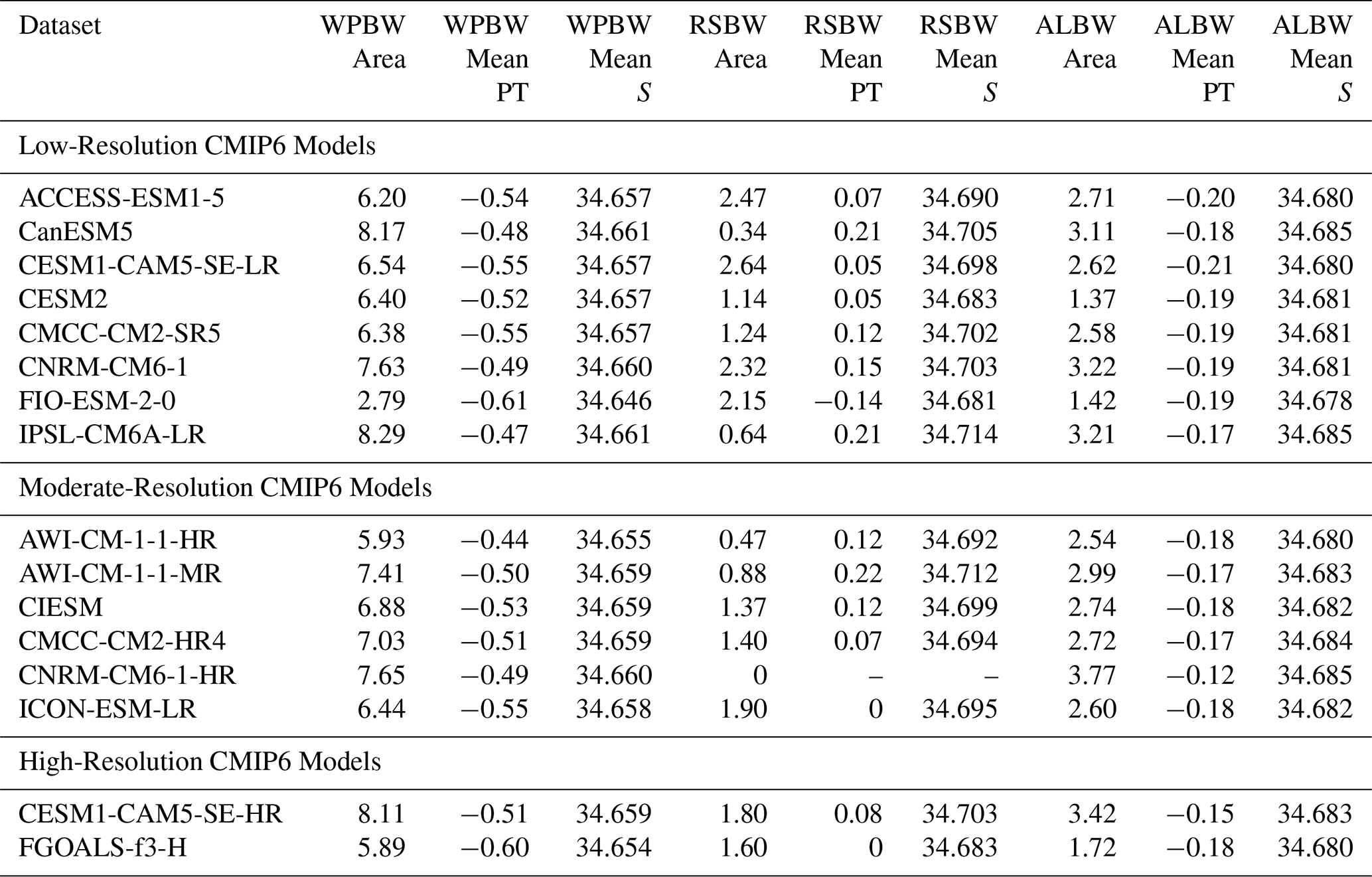
After applying the correction for potential temperature and practical salinity, many models identify larger areas of one or more AABW subtypes compared to their original simulations (Figs. 5 vs. 6), although their spatial distributions still differ from WOA23 and the ensemble reanalysis. Tables 5 and S3 summarize the statistics after the bias correction at the 4000 m and near-bottom layers, respectively. Figure 6 presents the same five representative models discussed in Sect. 3.3 (the complete bias-corrected results for all 16 CMIP6 models are provided in Figs. S7 and S8).

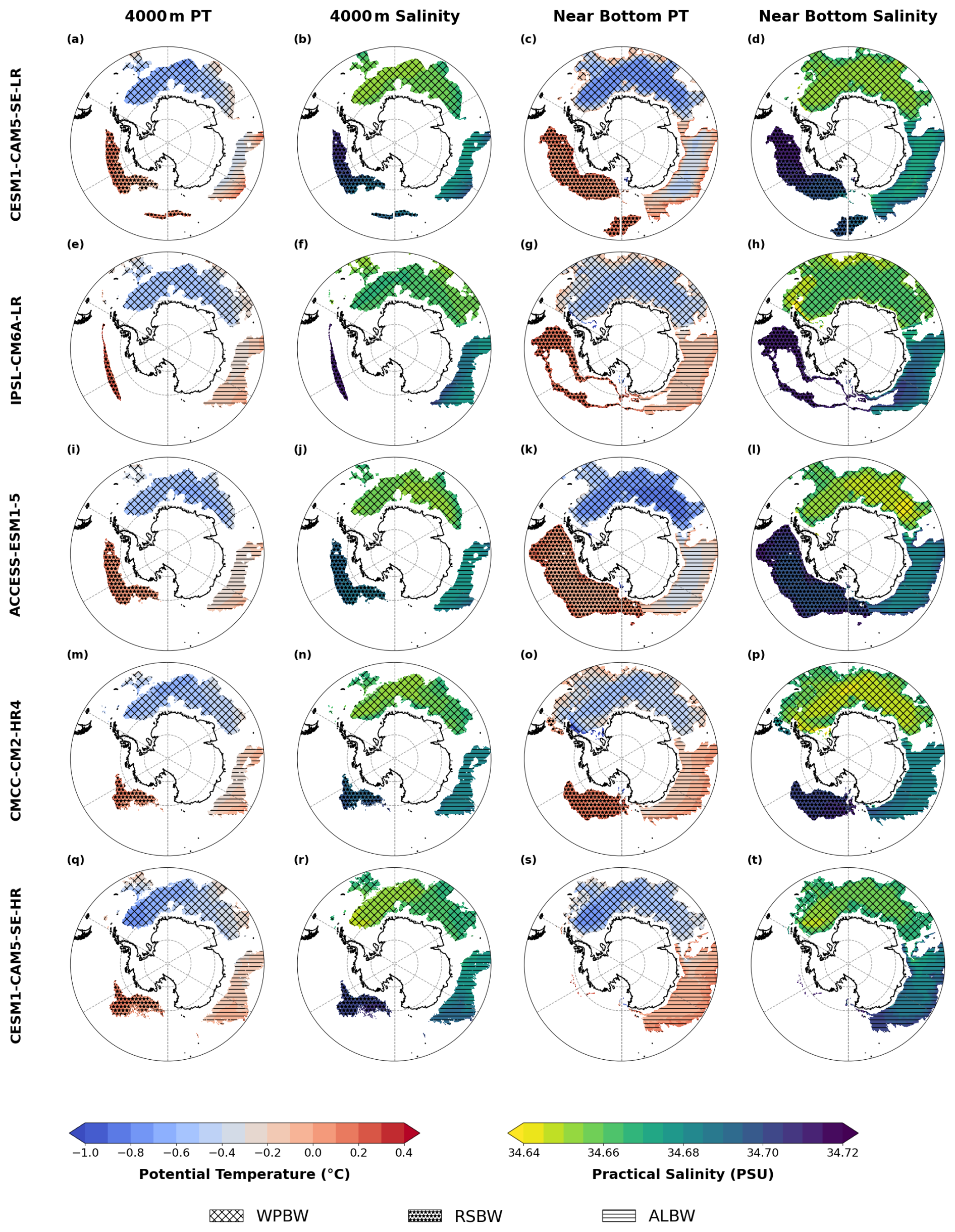
Figure 6 The bias-corrected potential temperature and practical salinity of AABW subtypes in the same five representative CMIP6 models shown in Fig. 5. The rows show CESM1-CAM5-SE-LR, IPSL-CM6A-LR, ACCESS-ESM1-5, CMCC-CM2-HR4, and CESM1-CAM5-SE-HR. The columns show potential temperature at 4000 m, practical salinity at 4000 m, potential temperature at the near-bottom layer, and practical salinity at the near-bottom layer. Subpanels are labeled from (a) to (t). The respective AABW subtypes are distinguished by distinct hatching patterns, as detailed in the figure legend. Complete bias-corrected spatial distributions for all 16 CMIP6 models are provided in Figs. S7 and S8.

Among the three representative low-resolution models, CESM1-CAM5-SE-LR changes little at 4000 m but shows clearer subtype-dependent changes in the near-bottom layer. At 4000 m, its WPBW, RSBW, and ALBW areas change from 6.39, 2.20, and 2.38 × 10⁶ km² to 6.54, 2.64, and 2.62 × 10⁶ km², respectively. This limited response is consistent with its original thermohaline state already permitting the identification of all three subtypes. At the near-bottom layer, the corresponding areas change from 10.07, 7.82, and 4.81 × 10⁶ km² to 10.58, 5.56, and 5.70 × 10⁶ km², respectively. The corrected ALBW area becomes closer to the WOA23 value, the RSBW area becomes smaller than the reference value, and the WPBW area changes only slightly (Figs. 5 and 6; Tables 4, 5, S2 and S3).

The IPSL-CM6A-LR model shows subtype-dependent responses at both depth levels. At 4000 m, its WPBW and ALBW areas change only slightly, from 8.30 and 3.42 × 10⁶ km² to 8.29 and 3.21 × 10⁶ km², respectively, whereas the RSBW area decreases from 3.53 to 0.64 × 10⁶ km². At the near-bottom layer, the WPBW, RSBW, and ALBW areas decrease from 14.95, 8.68, and 6.51 × 10⁶ km² to 13.53, 3.43, and 5.64 × 10⁶ km², respectively. Although the corrected ALBW area is close to the WOA23 value, RSBW becomes substantially underestimated. These results indicate that removing the regional mean bias does not consistently improve subtype extents and that the regional spatial contrasts retained by the model remain important (Figs. 5 and 6; Tables 4, 5, S2 and S3).

ACCESS-ESM1-5 identifies a very limited AABW distribution before the correction. At 4000 m, it identifies only 0.03 × 10⁶ km² of WPBW and no RSBW or ALBW. After the correction, the WPBW, RSBW, and ALBW areas increase to 6.20, 2.47, and 2.71 × 10⁶ km², respectively. At the near-bottom layer, the corresponding areas increase from 0.16, 0.02, and 0 × 10⁶ km² to 9.71, 8.53, and 5.50 × 10⁶ km², respectively. The corrected ALBW area is close to that in WOA23, whereas WPBW remains smaller and RSBW becomes larger than the corresponding WOA23 values. This substantial improvement indicates that the poor identification of AABW in ACCESS-ESM1-5 is strongly affected by the regional mean temperature and salinity biases, although the correction does not improve agreement with WOA23 uniformly across the three subtypes (Figs. 5 and 6; Tables 4, 5, S2 and S3).

For the representative moderate-resolution models, CMCC-CM2-HR4 responds strongly to the correction at both depth levels. At 4000 m, CMCC-CM2-HR4 identifies none of the three AABW subtypes in its original simulation, whereas after the correction, it identifies WPBW, RSBW, and ALBW areas of 7.03, 1.40, and 2.72 × 10⁶ km², respectively. At the near-bottom layer, the identified WPBW, RSBW, and ALBW areas increase from 0.07, 0.16, and 0.05 × 10⁶ km² to 12.68, 3.20, and 5.41 × 10⁶ km², respectively. After the correction, the WPBW and ALBW extents become broadly comparable to those in WOA23, whereas RSBW remains substantially underestimated. This indicates that regional mean biases strongly affect subtype identification (Figs. 5 and 6; Tables 4, 5, S2 and S3).

Among the representative high-resolution models, CESM1-CAM5-SE-HR also exhibits subtype- and depth-dependent responses. At 4000 m, its WPBW, RSBW, and ALBW areas change from 8.42, 1.24, and 0.10 × 10⁶ km² to 8.11, 1.80, and 3.42 × 10⁶ km², respectively. ALBW expands markedly, whereas RSBW remains smaller than that in WOA23. At the near-bottom layer, the corresponding areas change from 11.61, 3.20, and 0.44 × 10⁶ km² to 10.01, 0.14, and 6.27 × 10⁶ km², respectively. ALBW again expands substantially, but RSBW becomes nearly absent. This result indicates that a spatially uniform regional mean-state correction cannot compensate for all deficiencies in the simulated regional bottom-water structure (Figs. 5 and 6; Tables 4, 5, S2 and S3).

Beyond the five representative models, CNRM-CM6-1-HR provides a depth-dependent counterexample. At 4000 m, it identifies none of the three subtypes before correction. After the correction, its WPBW and ALBW areas increase to 7.65 and 3.77 × 10⁶ km², respectively, whereas RSBW remains absent. Near the bottom, however, none of the three subtypes is identified before correction, and only 0.01 × 10⁶ km² of ALBW is identified afterward. Its limited near-bottom response indicates that the absence of identified AABW at this depth cannot be explained solely by systematic regional mean biases (Tables 4, 5, S2 and S3).

Table 5 Quantitative metrics of the bias-corrected Antarctic Bottom Water (AABW) subtypes at the 4000 m depth layer across the Southern Ocean south of 50° S. The table lists the identified area (10⁶ km²), mean potential temperature (PT, °C), and mean practical salinity (S) of WPBW, RSBW, and ALBW for the 16 CMIP6 models. A value of 0 indicates that no grid cells satisfy the adopted subtype criteria after the regional mean-state correction. In such cases, the corresponding mean properties are denoted by dashes.

4 Discussion and conclusions

This study treats WPBW, RSBW, and ALBW as hydrographic subtypes and identifies them using consistent neutral-density, practical-salinity, and geographical criteria. The identification results reflect whether different datasets can reproduce the characteristic hydrographic states associated with the three AABW subtypes, rather than quantitatively attributing an individual water mass to a specific formation region.

For WOA23, RSBW is relatively warmer and more saline, WPBW is colder and fresher, and ALBW exhibits intermediate thermohaline properties. At the 4000 m and near-bottom layers, the areas of WPBW, RSBW, and ALBW identified by the ensemble reanalysis show good agreement with those of WOA23, with high spatial correlation.

Although current observations are not sufficient to accurately clarify the changes in the different types of AABW, some progress has been made. In the Weddell Sea, repeat hydrographic sections revealed pronounced decadal warming and freshening, together with reduced export of AABW (Jullion et al., 2013; Zhou et al., 2023). In Prydz Bay, CTD profiles collected by instrumented southern elephant seals showed that glacial meltwater can suppress dense shelf water formation and thereby affect local AABW production (Williams et al., 2016). More recent observations further suggest that local bathymetry and sea ice formation also influence this process (Portela et al., 2021, 2022). In the Ross Sea, a long-term freshening tendency was followed by a recovery in AABW salinity, density, and thickness since the 2010s (e.g., Silvano et al., 2020). In the Australian Antarctic Basin, AABW has undergone freshening and contraction, with the largest changes occurring near its source regions (van Wijk and Rintoul, 2014; Kobayashi, 2023). These observations demonstrate that AABW properties and their temporal evolution vary markedly among different Antarctic sectors. The WPBW, RSBW, and ALBW identified here should therefore be interpreted as climatological hydrographic categories representative of regional water mass characteristics, rather than as temporally invariant or unmixed source water endmembers.

The CMIP6 models exhibit substantial inter-model differences in subtype extent and thermohaline structure. Most CMIP6 models show poor identification of the three observed AABW subtypes. Some models (e.g., IPSL-CM6A-LR and CanESM5) identify extensive but biased subtype distributions, whereas others (e.g., ACCESS-ESM1-5, CESM2, and CMCC-CM2-HR4) identify only a small portion or no subtype distributions at all. Among the CMIP6 models, CESM1-CAM5-SE-LR reasonably reproduces the general distribution of the three subtypes.

The regional thermohaline mean-state bias correction improves subtype identification in some CMIP6 models, but the degree of improvement varies among models and subtypes. Such differences are not unexpected because AABW properties reflect a combination of processes associated with dense shelf water formation, freshwater forcing, overflow, entrainment, mixing, and downstream spreading, many of which remain challenging to represent in global climate models (Silvano et al., 2018, 2023; Han et al., 2024, 2025; Heuzé, 2021). Some improvements after the bias correction are consistent with an important contribution from regional thermohaline mean-state offsets, whereas limited or non-uniform improvement suggests that deficiencies in the retained spatial structure may also be important. Because the correction is diagnostic and preserves the models' spatial anomaly patterns, the remaining biases cannot be attributed to specific physical processes. Nevertheless, the contrasting correction responses help distinguish deficiencies associated with the regional mean state from those that persist in the simulated spatial structure. Future work will extend this evaluation of AABW subtypes to emerging global climate model simulations with ocean grid spacing of approximately 5 km (Rackow et al., 2025; Kang et al., 2026). These simulations will help assess whether improved representation of shelf and slope processes reduces the deficiencies identified here in AABW formation, export, and spatial structure, or whether these deficiencies persist because of other aspects of model formulation.

Beyond the climatological comparison described above, Fig. S9 reveals clear differences among the datasets in subtype areas and their temporal evolution. Nevertheless, near-bottom RSBW declines overall in both the Ensemble Reanalysis and CESM1-CAM5-SE-LR, consistent with the slight decrease in the WOA23 period-mean estimates. For WPBW, the Ensemble Reanalysis and CESM1-CAM5-SE-LR show relatively smooth interannual variations, while the corresponding WOA23 period-mean estimates change only slightly. Future work should clarify the sources of these differences and improve cross-dataset comparability.