Chlorophyll a variation trends in marginal seas: assessing the impact of global warming and anthropogenic activities using time-series satellite data (1998–2020)

Global warming has been identified as the primary cause of the decline of surface chlorophyll a (Chl a) concentrations in the oceans. Conversely, increasing Chl a concentrations have been observed in a number of marginal seas over recent decades due to the increasing anthropogenic input of key nutrients. With the intensification of global warming, however, its impact on Chl a in coastal waters along with the superimposed effects of human regulation of nutrients emissions has been rarely studied. To address this research gap, in this study, we provided a comparative analysis of enclosed versus open marginal seas, revealing divergent physiological and ecological responses to rising sea-surface temperature (SST) across different nutrient regimes. We utilized time series of ocean color satellite data from 1998 to 2020 to examine the spatiotemporal distribution of Chl a in a range of marginal seas, and we considered its relationship with environmental factors, in particular with SST, photosynthetically active radiation (PAR), and surface wind speed (SWS). The results suggested that the sea areas examined, with their varying mixing and water exchange characteristics and degrees of human influence, have had different responses in terms of their Chl a trends to increasing SST. Specifically, in eutrophic enclosed seas with weak hydrodynamic exchange capacity, such as the Bohai Sea, increasing SST did not suppress Chl a concentration; instead, we observed a continuous increase in Chl a in the center of the sea. In comparison, the open marginal seas examined showed strong negative relationships between SST and Chl a with increasing distance offshore regardless of the degree of pressure from human activities. This result indicated that the expected global warming effects driving reductions in Chl a have been extending to nearshore and marginal sea areas. This trend may be exacerbated by stricter environmental management policies imposed in recent years, which have reduced anthropogenic nutrient input. Distinct from the noted effect of global warming, PAR and SWS have shaped Chl a in ways that are strongly modulated by geography and climate. PAR is the dominant positive driver only in the Amazon Estuary, where equatorial cloudiness and high turbidity create a light-limited regime, so any increase in PAR directly stimulates phytoplankton. In mid-latitude open waters, PAR is secondary to SST. Its seasonal rise is coupled to SST and therefore it is negatively correlated with Chl a after thermal stratification reduces nutrient supply. SWS has emerged as a key driver in the three open regimes (the East China Sea > the Eastern Coastal Waters of the United States > the Amazon Estuary) by injecting nutrient-rich cold deep water and episodically raising Chl a. Inside the two enclosed seas (the Bohai Sea and the Gulf of Mexico), correlations with both PAR and SWS have been weak ($\left|r\right|$ < 0.2). Thus, the control PAR and SWS exert over Chl a is complex, but both are linked to SST and nutrient input. In this study, we highlighted the complex interactions among primary production, SST, nutrient input and hydrodynamic exchange, and environmental protection controls under the dual pressures of changes in human activity and coastal development combined with global warming.

1 Introduction

Marine phytoplankton account for approximately half of Earth's primary productivity and play a key role in ocean biogeochemical cycles and global climate processes (Field et al., 1998). Biological carbon pump (BCP) marine phytoplankton account for about 26 % of the global carbon sink (Dai et al., 2022; Friedlingstein et al., 2022; Jin et al., 2020; Letscher et al., 2023). Phytoplankton biomass is a key index for monitoring marine ecology and environments, as it facilitates accurate estimation of oceanic primary productivity, carbon sinks, and food security.

Numerous studies have indicated that an observed decline of phytoplankton biomass over the past century in global oceans can be attributed to increasing sea surface temperature (SST) as a result of global warming (Baker and Geider, 2021; Behrenfeld et al., 2016; Boyce et al., 2010; IPCC, 2021). Since the beginning of the 20th century, a rise in SST (specifically, an average temperature increase of 0.6 °C in the upper ocean) has led to the strengthening of water column stratification. This has limited vertical nutrient exchange, resulting in reduced nutrient concentration in upper waters, which in turn has limited phytoplankton growth (Mizuta and Wikfors, 2020). It has been estimated that 80 % of the observed decline in marine phytoplankton biomass from 1899 to 2008 is related to climate change, with the rate of chlorophyll a (Chl a) concentration reduction increasing with distance from the coast (Boyce et al., 2010). In the Pacific and Atlantic Oceans in particular, from 1998 to 2007, waters with a low Chl a concentration (Chl a ≤ 0.07 mg m⁻³) expanded at an annual rate of 0.8 %–4.3 %, replacing approximately 800 000 km² of water with a high Chl a concentration each year (Gregg et al., 2005; Gregg and Rousseaux, 2014). Additionally, as one of the most prominent sources of interannual natural variability in Earth's climate system, global warming may alter the frequency and intensity of El Niño–Southern Oscillation (ENSO) events, thereby inducing extensive positive or negative SST anomalies across the Pacific and beyond. Global warming has introduced additional complexity in deciphering the SST–Chl a concentration relationship at regional and interannual scales (Cai et al., 2022; Hou et al., 2024).

Despite the global rise in SST, near-shore phytoplankton biomass has been increasing, which is believed to be the result of anthropogenic eutrophication (Boyce et al., 2010; Jickells, 1998; Kong et al., 2019; Lee et al., 2019; Marrari et al., 2016). Regional studies have presented conflicting conclusions regarding the relationship between SST and Chl a in coastal waters, which may be due to various regional oceanographic and anthropogenic effects. Coastal regions with upwelling, such as the Eastern North Atlantic (Siemer et al., 2021) and Bay of Bengal (Chowdhury et al., 2021), have exhibited a seasonally dependent, negative correlation between Chl a and SST. In these regions, notwithstanding land-derived nutrient input, upwelling has played a crucial role in transporting colder, deeper water with abundant nutrients to the sea surface, stimulating local phytoplankton populations and resulting in this negative correlation between SST and Chl a (Chen et al., 2021; Favareto et al., 2023). This natural physical control, however, can be masked or even reversed in coastal systems where anthropogenic pressures dominate. In such areas, despite increases in SST, nutrient runoff and other anthropogenic activities have exacerbated primary productivity from the mid-20th century onward. For example, in the Baltic Sea, an increase in cultural eutrophication since the 1950s has produced marked sedimentary changes in a range of organic geochemical indicators. These indicators, including those reflecting increased phytoplankton biomass, have been suggested to be important secondary markers for the proposed Anthropocene epoch at the candidate Global Boundary Stratotype Section and Point site (Kaiser et al., 2023). Other anthropogenically enhanced processes have profoundly altered the correlation between Chl a and SST. These include predation pressure, particularly in aquaculture areas where filter-feeding organisms reduce phytoplankton biomass (e.g., Frau et al., 2021; Mao et al., 2020), and commercial fishing, which indirectly affects phytoplankton biomass by altering zooplankton and fish abundance (Campos-Silva et al., 2021; Reid et al., 2000).

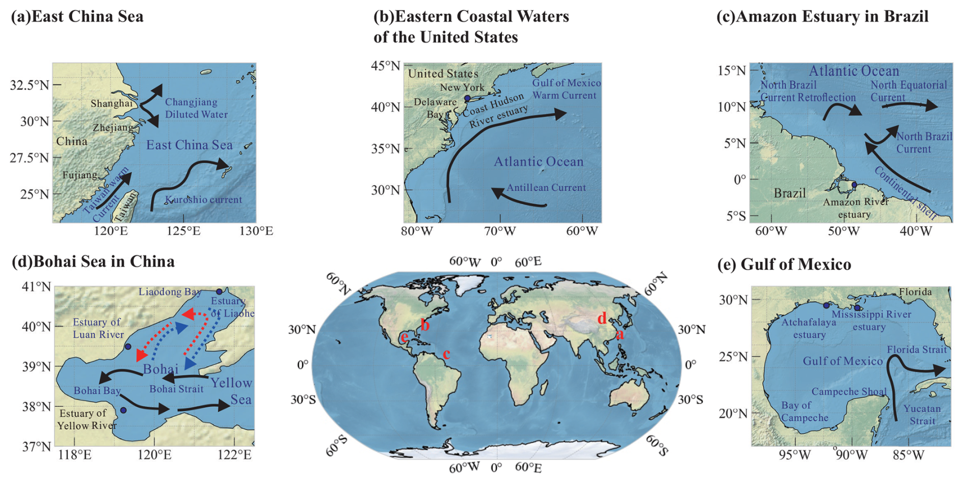
Figure 1 The geographic locations and major current systems of the five studied sea areas: (a) the East China Sea located in the range of 117–131° E and 23–33° N; (b) the Eastern Coastal Waters of the United States located in the range of 81.6–57.66° W and 27.5–43.3° N; (c) the Amazon Estuary located in the range of 16° N–6° S and 61–37° W; (d) the Bohai Sea located in the range of 37–41° N and 117–123° E; and (e) the Gulf of Mexico located in the range of 17.09–31.16° N and 98.86–81.28° W. Note: The base maps for the land and ocean portions of the map artifacts are land-cover data and ocean polygon data (rendered in gray) and are available for download from Natural Earth (https://www.naturalearthdata.com, last access: 25 May 2026).

In addition, the complex responses of photosynthetically active radiation (PAR) and surface wind speed (SWS) to global warming exert additional influence on upper-layer Chl a, making it difficult to clarify the impact of warming independent of these concurrent physical changes. Photophysiological processes – namely photoinhibition under supersaturating irradiance and photoadaptation through adjustments in pigment composition, light-harvesting complex abundance, and non-photochemical quenching capacity – exert first-order control on upper-ocean Chl a inventories (Moradi and Moradi, 2020; Pi et al., 2019). Despite large-scale previous efforts, however, significant gaps remain in the current understanding of the variability of Chl a and its relation to the PAR on regional seasonal time scales. The influence of SWS on Chl a is nonlinear and spatially heterogeneous (Feng et al., 2015; Kahru et al., 2010; Lin et al., 2023). Broadly, moderate SWS intensifies coastal upwelling, injecting nutrient-rich deep water into the euphotic zone and stimulating phytoplankton growth. In contrast, excessive wind forcing deepens the mixed layer and shortens residence time, thus impeding phytoplankton retention in the illuminated layer and ultimately suppressing biomass accumulation. Moreover, the magnitude and the sign of this relationship vary with regional circulation and seasonal stratification (Wang and Xiu, 2022).

To better understand the drivers of temporal and spatial Chl a concentration trends in coastal waters, in this study, we assessed the relationship between Chl a concentrations (a proxy for phytoplankton biomass) and SST in five coastal waters with varying levels of anthropogenic activity, using time-series satellite data from 1998 to 2020. We also incorporated indices, including PAR and SWS, to comprehensively explore the underlying mechanisms driving the evolution of Chl a. Specifically, we examined two enclosed bays with high levels of human interference (the Gulf of Mexico in the United States and the Bohai Sea in China), and three open-sea areas with varying degrees of human interference (the Amazon Estuary, the Eastern Coastal Waters of the United States, and the Changjiang Estuary). The objective of this study was to elucidate the distinct responses of phytoplankton to sustained global warming in the presence of anthropogenic nutrient input and to distinguish the ecological effects of warm water intrusion from those of human activities.

The remainder of this paper is structured as follows. In the Data and Methods section, we describe the study areas, satellite data sources, and the methodologies employed, including trend analysis, stability assessment, and correlation analysis. In the Results section, we present the spatiotemporal distribution characteristics of Chl a, its historical variation trends, stability, and its relationship with key environmental factors across the five marginal seas. On the basis of these findings, in the Discussion, we provide a comprehensive analysis of the mechanisms driving Chl a variations, focusing on the roles of natural environmental factors, global warming, and anthropogenic nutrient input. Finally, in the Conclusions, we summarize the main findings of the study and discuss their ecological implications under the dual pressures of global warming and human activity.

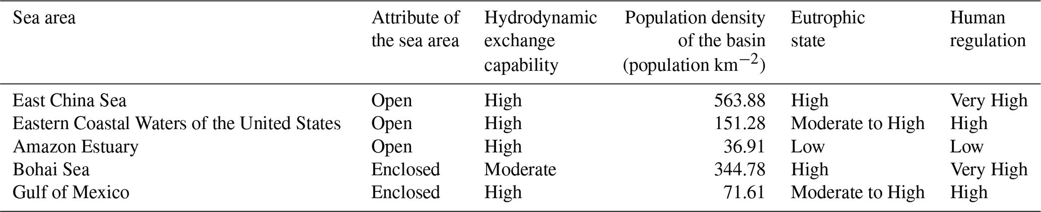
Table 1 Comparative environmental and demographic overview of study regions.

2 Data and Methods

2.1 Study Areas

In this study, we focused on five marginal seas around the world with different water-exchange rates and levels of anthropogenic activity (Fig. 1) (Cui et al., 2021; Dobson et al., 2000; Lloyd et al., 2019). Enclosed seas (in this study, the Bohai Sea and the Gulf of Mexico) are typically characterized by particularly slow water exchange, which limits the diffusion and transportation of land-sourced pollutants and produces a limited self-purification capability. The three open-sea areas included in this study were the Changjiang Estuary, the Eastern Coastal Waters of the United States, and the Amazon Estuary. In this study, we defined an open-sea area relative to the enclosed-sea area, that is, a near-shore area with only one land boundary. Generally, the hydrodynamic conditions in open-sea areas are favorable for the diffusion of land-derived materials.

The East China Sea is one of the largest marginal seas of the northwestern Pacific, with complex circulation systems (Fig. 1a). The Tsushima and Kuroshio currents, with high temperatures and salinities, prevail in the eastern side of the East China Sea. On the western side, the Zhemin Coastal Currents, formed by the Changjiang River Plume with the intrusion of the Taiwan Warm Current, dominate. Due to increasing human activities in the Changjiang River Basin, nutrient input has increased significantly, leading to more frequent harmful algal blooms (HABs) (Ministry of Ecology and Environment, PRC, 2001, 2021; Zhou et al., 2022).

The Eastern Coastal Waters of the United States, located to the northeast of the Gulf of Mexico, are strongly influenced by the Gulf Stream, resulting in enhanced primary productivity (Ma and Smith, 2022). Numerous rivers, including the Hudson, Delaware, Susquehanna, and Joptank rivers, which flow through highly urbanized cities, discharge pollutants and have increased the frequency of HAB events in the past decades (e.g., Mizuta and Wikfors, 2020).

In the Amazon Estuary, the tropical Atlantic surface circulation, specifically the North Brazil Current running north-westward along the Brazilian coastline, exerts a dominant influence over the area (Fig. 1c). The Guyana Current is also active in this sea area. HABs in the Amazon Estuary typically occur during the spring and summer, influenced by the seasonal flow variations of the Amazon River. Notably, HAB events have increased since 2008 (Dai et al., 2023; Hallegraeff et al., 2021; Subramaniam et al., 2008).

The Bohai Sea has been undergoing severe anthropogenic disturbance with coastal runoff from at least 40 rivers, including the Yellow River, Haihe River, and Liaohe River. The influx of significant amounts of pollutants, including sewage, has severely disrupted the local aquatic ecology (Ministry of Ecology and Environment, PRC, 2021). The circulation of the Bohai Sea exhibits seasonal variations (Fig. 1d), which has significantly affected pollutant transport (Wu et al., 2023; Zhang et al., 2018). The rate of seawater exchange with the Yellow Sea has strongly influenced the ecological environment within the Bohai Sea (Ju et al., 2020).

The circulation system in the southeast of the Gulf of Mexico (Fig. 1e) acts as its primary hydrodynamic force, stimulating the local primary productivity (Damien et al., 2021). In contrast, the northern part of the Gulf of Mexico is significantly influenced by nutrient input originating from the Mississippi–Atchafalaya Basin. Accelerated industrial growth and extensive fertilizer use have led to the excessive production of algae (e.g., Fu et al., 2020; Yingling et al., 2022).

The five selected sea areas cover varying degrees of human activity and hydrodynamic exchange capability, as summarized in Table 1. We obtained population density data for the surrounding basins from the LandScan (2020) high-resolution global population dataset (Lebakula et al., 2025), which we used as a proxy for anthropogenic pressure. In this context, the term “Human regulation” quantifies the intensity of human activities within the basin that regulate nutrient input and environmental stress on the marine ecosystem. Because long-term, internally consistent time-series datasets of riverine total nitrogen and total phosphorus fluxes were not available for all five study regions over the entire analysis period (1998–2020), we did not include quantitative nutrient loading as an explanatory variable in this comparative analysis.

Table 2 Monthly satellite-derived datasets used in this study.

2.2 Data Sources

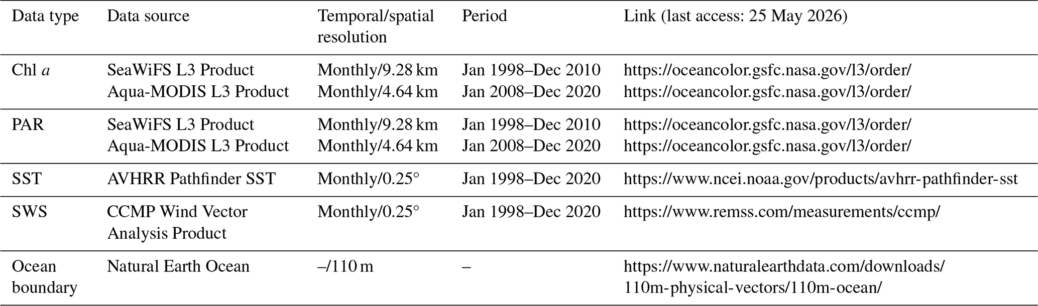
Regarding the various chemical, hydrological, meteorological, and biological factors, satellite-derived datasets with Chl a, SST, PAR, and SWS data were used to evaluate temporal and spatial variation trends and interactions (Hong et al., 2023; Martinez et al., 2020; Xi et al., 2021). SST was used to identify periods in which the seawater was heated, and PAR and SWS were included as the key environmental indices known to influence phytoplankton growth and distribution. PAR directly constrains photosynthesis, whereas SWS affects vertical mixing, nutrient entrainment from deeper layers, and light availability by modulating the mixed-layer depth. Table 2 shows the types of data, data sources, temporal and spatial resolution, spanning periods, and download websites used in this study.

We selected these datasets, derived through algorithmic processing of raw satellite imagery, for their reliability and comprehensive temporal coverage, which made them particularly valuable for studying waters with complex optical properties, such as coastal and estuarine environments (Pisano et al., 2016; Zhang et al., 2006). We applied a consistent preprocessing method (see Sect. 2.3) to establish a unified satellite dataset from multiple satellites. Taking Chl a and PAR as examples, before constructing the time-series dataset, we divided the satellite Chl a and PAR data into the following three periods according to availability of different satellite products: T1 period: January 1998–December 2002, Chl a and PAR products were only available from the Sea-Viewing Wide Field-of-View Sensor (SeaWiFS); T2 period: January 2003–December 2010, overlap period, Chl a and PAR products were available from both the Moderate Resolution Imaging Spectroradiometer (MODIS) and SeaWiFS; and T3 period: January 2011–December 2020, Chl a and PAR products were available only only from MODIS. Because the two satellite sensors (SeaWiFS and MODIS) had different operational periods, we eliminated systematic errors before merging them into a long-term dataset. See Appendix A for an in-depth explanation of the data preprocessing methodology. We extracted the SST data from the AVHRR Pathfinder dataset (Pisano et al., 2016). Additionally, we incorporated SWS data from the Cross-Calibrated Multiplatform (CCMP) Wind Vector Analysis Product (Mears et al., 2019). All datasets used in this study were last accessed on 25 May 2026.

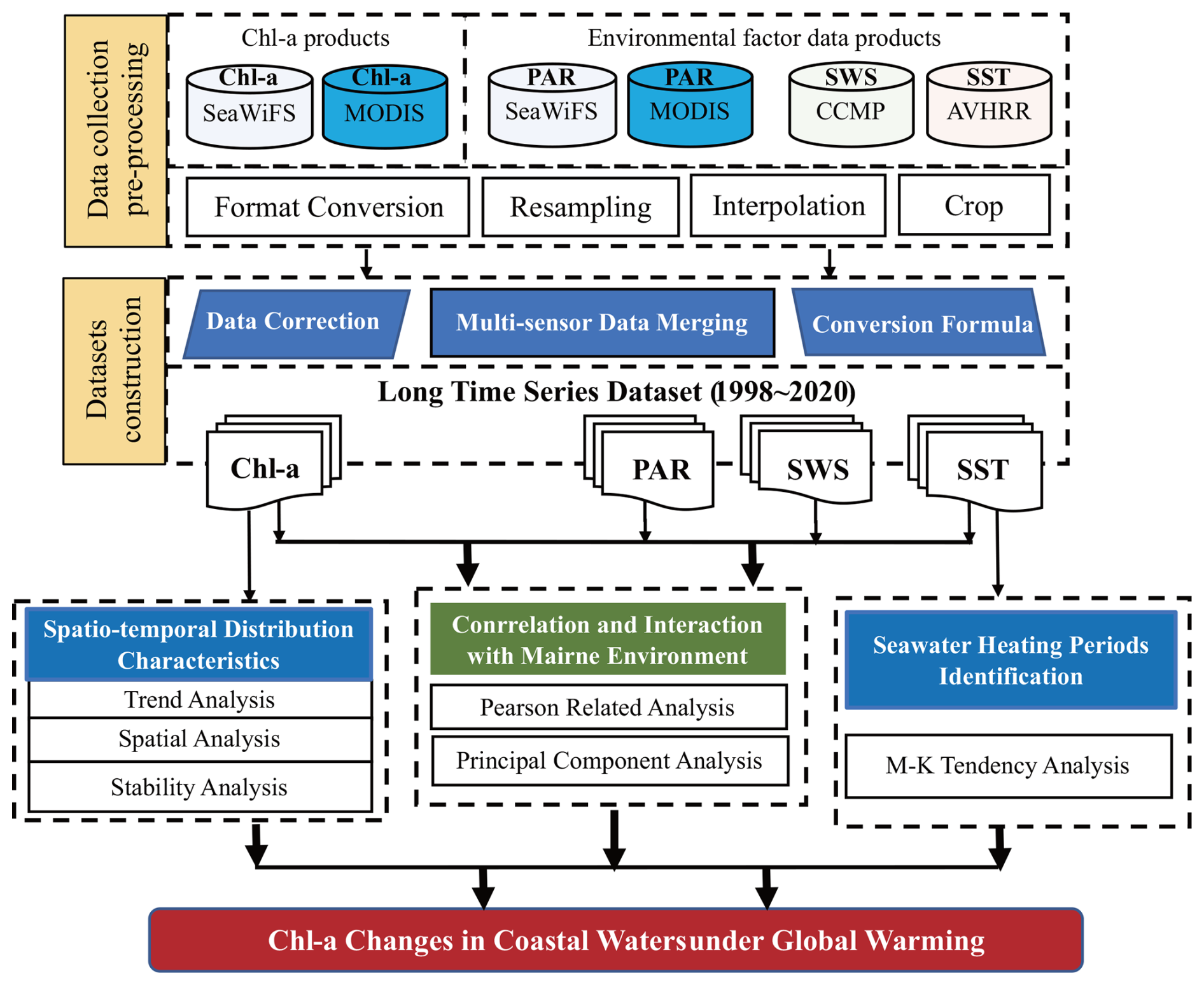
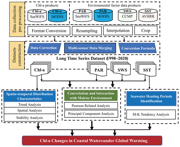
Figure 2 Flowchart of assessing the impact of global warming and anthropogenic activities on Chl a concentration trends using time-series satellite data.

2.3 Methods

Figure 2 shows a flowchart of this study. To harmonize datasets with different spatial resolutions, we reprojected and resampled all the raster datasets to a common reference grid before further analysis. We used a MODIS grid file covering the study areas as a spatial reference, and resampled the Chl a, PAR, SST, and SWS datasets using bilinear interpolation with the GDAL Warp function. This procedure ensured that all variables had consistent projection, pixel size, and spatial extent. We then used the temporally matched monthly datasets for subsequent analyses. Regarding the availability of satellite datasets for Chl a, PAR, SWS, and SST (1998–2020), we determined the correlation and interaction between changes in Chl a concentration and seawater warming according to the following steps: (1) We analyzed the temporal trends of seasonal and annual Chl a concentrations in the five study areas using the Mann–Kendall (M-K) trend analysis method. (2) We calculated Chl a stability and the coefficients of variation for each pixel, the varying degrees of Chl a concentrations, and conducted correlation analyses and principal component analyses (PCA) to determine the predominant marine environmental factors affecting Chl a concentrations in each sea area. (3) We identified global warming periods using the SST dataset. (4) We calculated the image-by-image metric correlations between Chl a and anthropogenic rising SST for specific time periods of interest.

2.3.1 Time-series analysis

We applied the least squares method, widely used in time-series analyses related to climate change (Mudelsee, 2019), to obtain trends in Chl a concentration over the period 1998–2020. The time series for trend analysis was composed of Chl a concentration values for each pixel in the study areas, with outliers removed if they exceeded three times the standard deviation from the mean (see Appendix B for calculation details). We used the obtained results to assess the local Chl a response to global warming.

Table 3 Discrimination criteria for M-K test.

Note: α represents the level of confidence.

The M-K trend analysis method is a nonparametric statistical approach widely employed to discern temporal trends in time-series data (e.g., Wang et al., 2021). This method can be used to assess whether there is a statistically significant increasing or decreasing trend by comparing the relative ranks of data points over time. We calculated the test statistic upward factor (UF) to identify the sequence of potential upward trends, and we derived the downward factor (DF) from the reversed data series to pinpoint the timing of potential trend shifts. The formulas for UF and UB are as follows:

$$\begin{array}{}\text{(1)}& {\displaystyle }& {\displaystyle }{\text{UF}}_k={\displaystyle \frac{s_k-E\left(s_k\right)}{\sqrt{\text{Var}\left(s_k\right)}}},(k=\mathrm{1},\mathrm{2},\mathrm{\dots },n),\text{(2)}& {\displaystyle }& {\displaystyle }{\text{UB}}_k={\displaystyle \frac{E\left(s_k\right)-s_k}{\sqrt{\text{Var}\left(s_k\right)}}},(k=\mathrm{1},\mathrm{2},\mathrm{\dots },n),\end{array}$$

where s_k is a statistical measure defined in the M-K test; Var(s_k) represents the variance of the calculated statistical measure; and E(s_k) represents the expected value of the statistical measure. The relevant calculation formulas are provided in Appendix C.

In the M-K test, the null hypothesis of no trend was rejected at the 5 % significance level if the absolute value of UF exceeded 1.96. A positive UF value indicated an upward trend, whereas a negative value indicated a downward trend. The intersection point of the UF and UB curves, if it occurred within the confidence limits, suggested a potential abrupt change in the trend for the year. The detailed discrimination criteria for trend significance and direction are summarized in Table 3.

2.3.2 Spatiotemporal trends analysis

We employed the slope analysis method (Wang, 2006) to analyze the spatiotemporal trends of Chl a in the five study areas. From 1998 to 2020, we calculated the annual variation rates of Chl a according to the least squares method using time-series data from each pixel within the study regions. A slope > 0 indicated an upward trend of Chl a at the corresponding pixel, and vice versa. The larger the value, the faster the increase (see Appendix C for details).

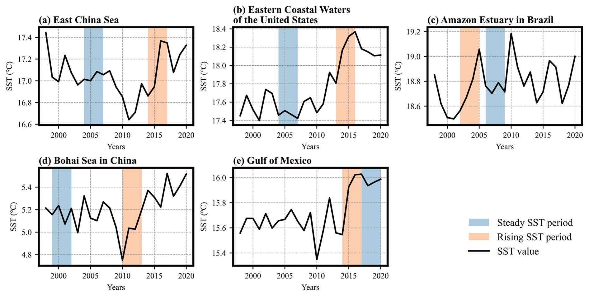
Figure 3 SST variation in the five study areas from 1998 to 2020, with identified periods of SST rise and stability.

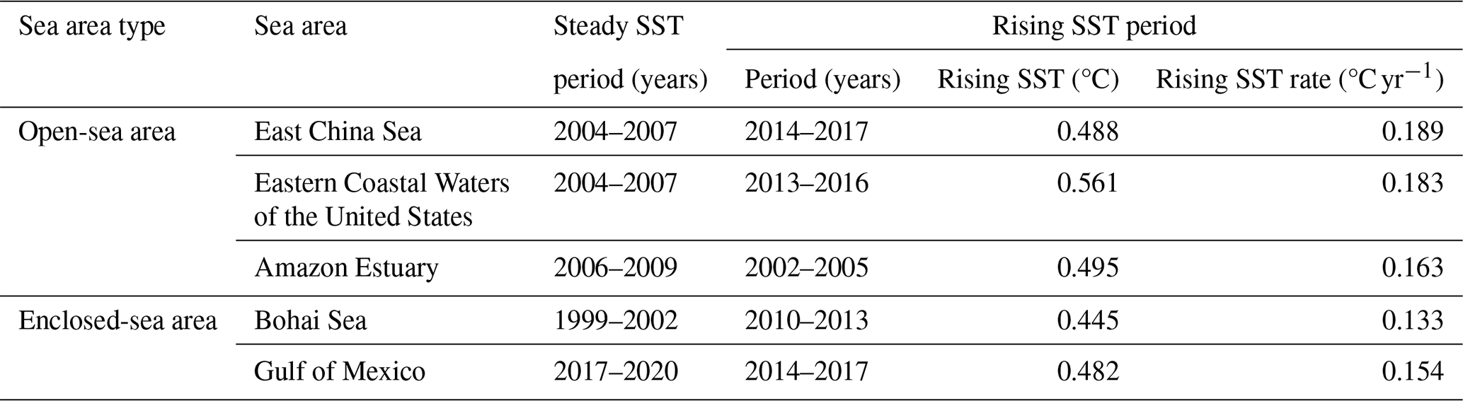
Table 4 Periods identified with different SST variation trends.

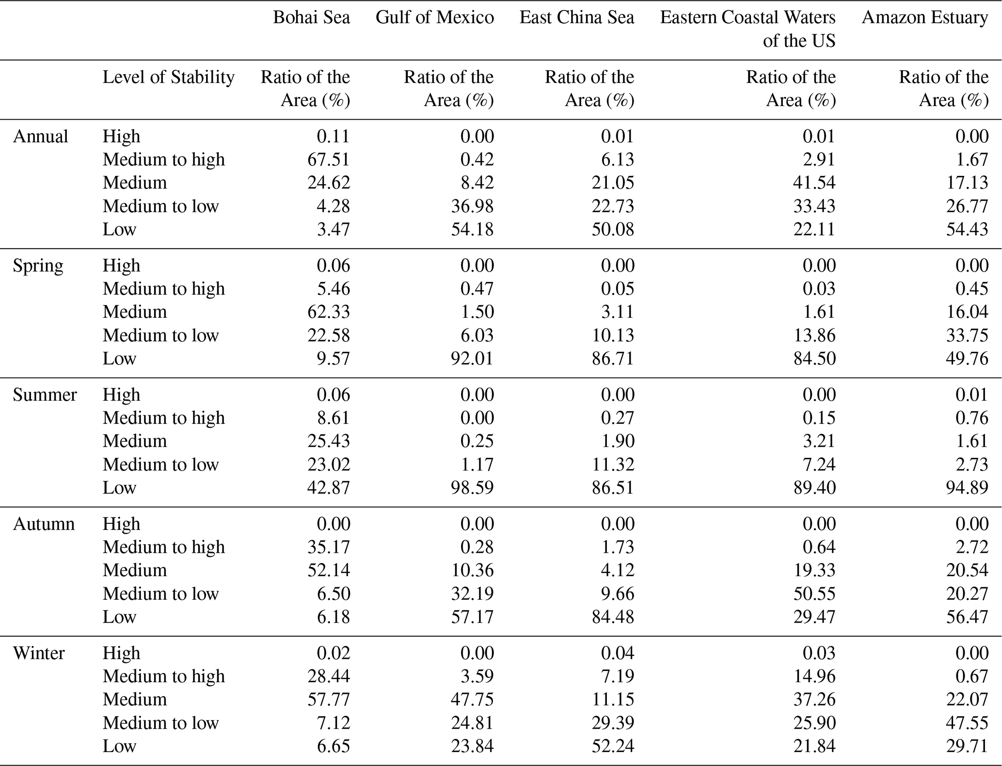
We calculated the stability of Chl a by computing the coefficient of variation (CV) of Chl a time-series data for each pixel. We classified the Chl a stability into five levels based on CV values: “High Stability” (CV < 0.05) indicated minimal variability; “Medium to High Stability” (0.05 ≤ CV < 0.10) reflected minor fluctuations; “Medium Stability” (0.10 ≤ CV < 0.15) showed moderate variability; “Medium to Low Stability” (0.15 ≤ CV < 0.20) represented significant fluctuations; and “Low Stability” (CV ≥ 0.20) signified highly unstable conditions (see Appendix D for details).

2.3.3 Seawater heating period identification

We identified the warming periods based on SST changes during 1998–2020 in the five study areas using a 4-year moving time window (Fig. 3). We selected this window length to capture sustained, low-frequency warming signals indicative of climate-scale changes, while smoothing out shorter-term interannual variability (e.g., those linked to seasonal cycles or transient weather events). We selected periods exhibiting the most pronounced rise in SST within this 4-year window to analyze the interaction between Chl a and SST increase. For comparison, we identified periods of relatively stable SST using the same 4-year window methodology.

The two time windows identified with the largest rise in SST and the most stable SST in the five study areas are shown in Table 4. The largest rising SST periods exhibited significant variation, reaching up to 0.120–0.200 °C yr⁻¹. In contrast, the most stable SST periods corresponded to variations of approximately 0.005–0.010 °C yr⁻¹. The main rising SST periods for the Gulf of Mexico, the East China Sea, and the Eastern Coastal Waters of the United States aligned with the time windows of the most intense El Niño event recorded (2014–2016), whereas distinct rises in SST for the Amazon Estuary and the Bohai Sea were coincident with the occurrence of the El Niño windows of 2002–2003 and 2009–2010, respectively (Cai et al., 2021; https://www.cpc.ncep.noaa.gov/products/analysis_monitoring/ensostuff/ONI_v5.php, last access: 25 May 2026).

2.3.4 Correlation analysis

We performed Pearson correlation and PCA to identify the impacts of environmental factors on Chl a concentrations for each study area. Specifically, to better understand how global warming affected phytoplankton in coastal seawaters, we completed a quantitative determination of the correlation between Chl a concentrations and SST for each pixel within the study areas in the rising and stable SST periods, respectively (Maćkiewicz and Ratajczak, 1993). For PCA, we first spatially averaged monthly raster data of Chl a, SST, PAR, and SWS over valid pixels within each study area to obtain regional monthly mean series, which we then normalized using min–max normalization. We conducted PCA on these normalized regional time series to identify the dominant environmental gradients associated with Chl a variability. The time-series data for annual mean Chl a and SST were normalized to address their inherent non-normal distribution. By comparing the changes in correlations between Chl a and SST across the different sites, under conditions of thermal variation and stability, and while considering the local hydrological characteristics, we delved into the mechanisms by which global warming influenced Chl a.

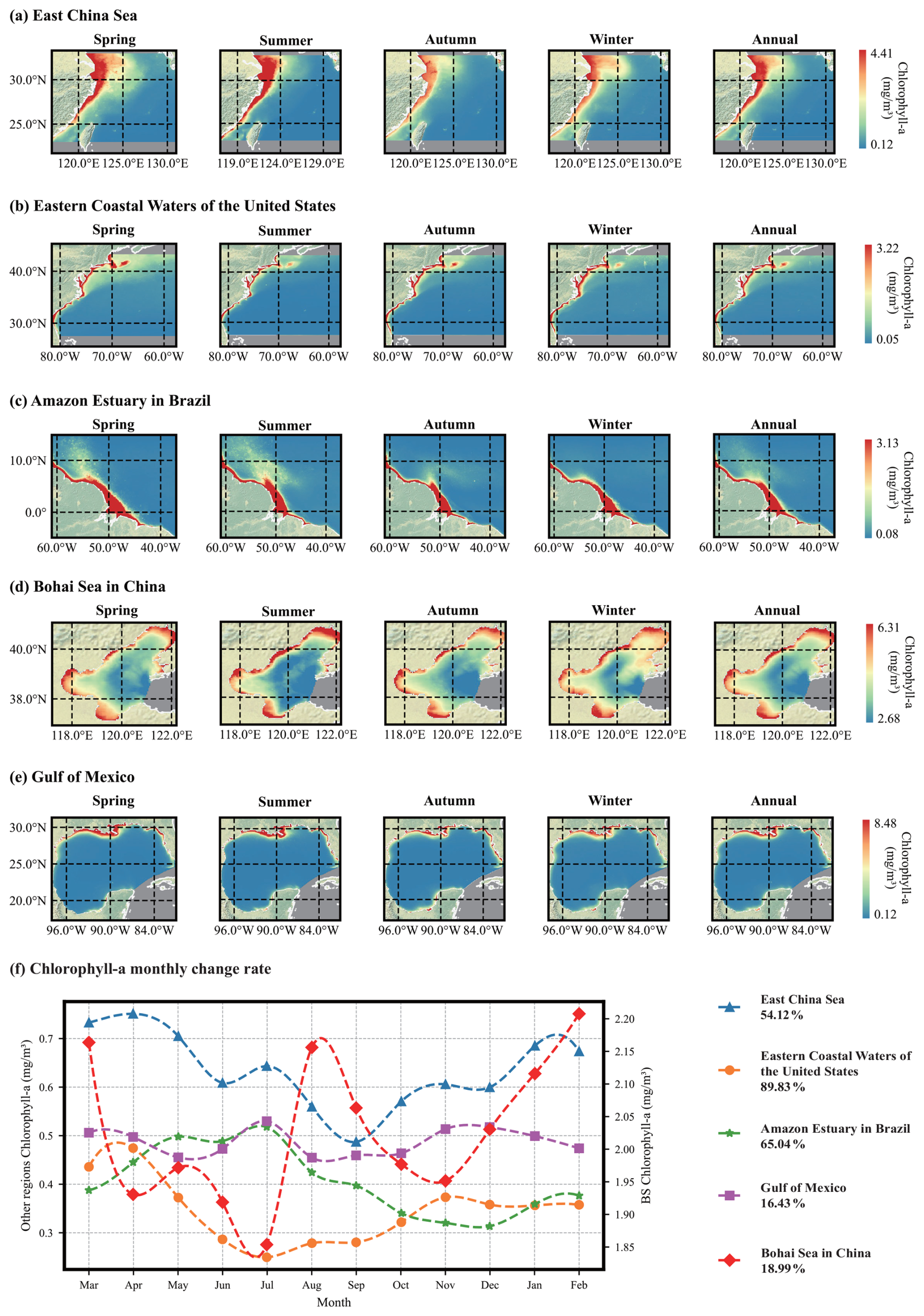
Figure 4 Spatial distribution of annual and seasonal Chl a concentrations at the five sites: (a) the East China Sea, (b) the Eastern Coastal Waters of the United States, (c) the Amazon Estuary, (d) the Bohai Sea, and (e) the Gulf of Mexico. (f) Monthly variation of Chl a concentrations. The Bohai Sea is shown on the right y-axis, whereas the other four seas are shown on the left y-axis. The data on the right are the monthly change rates. Areas shown in light gray-blue indicate missing data.

3 Results

3.1 Spatial Distribution Characteristics of Chl a

Figure 4 shows the seasonal and annual spatial distribution of Chl a concentrations for the five study areas. All the study areas showed distinct trends of decreasing Chl a concentrations as the distance offshore increased, and higher values were observed primarily in the estuaries and bays. In particular, areas with higher Chl a were more uniformly distributed in the Bohai Sea with limited water exchange, whereas the Gulf of Mexico, although morphologically classified as an enclosed sea, showed a more similar spatial distribution tendency to the open-sea areas because of its strong water exchange with the Atlantic.

Chl a concentration varied from greatest to least as follows: Bohai Sea > East China Sea > Gulf of Mexico > Eastern Coastal Waters of the United States ≈ Amazon Estuary. As a severely eutrophic enclosed-sea area, the Bohai Sea maintained high values between 1.6 and 2.5 mg m⁻³ throughout the year. Meanwhile, the East China Sea, which is a highly eutrophic open-sea area, exhibited a consistently higher annual Chl a, with spring values frequently exceeding 0.6 mg m⁻³. The other three regions all had year-round Chl a below 0.6 mg m⁻³. Chl a concentrations in the open-sea area exhibited greater susceptibility to seasonal variation than those in enclosed-sea areas with restricted exchange, as shown in Fig. 4f. Changes in the monthly average rate of Chl a concentration surpassed 50 %.

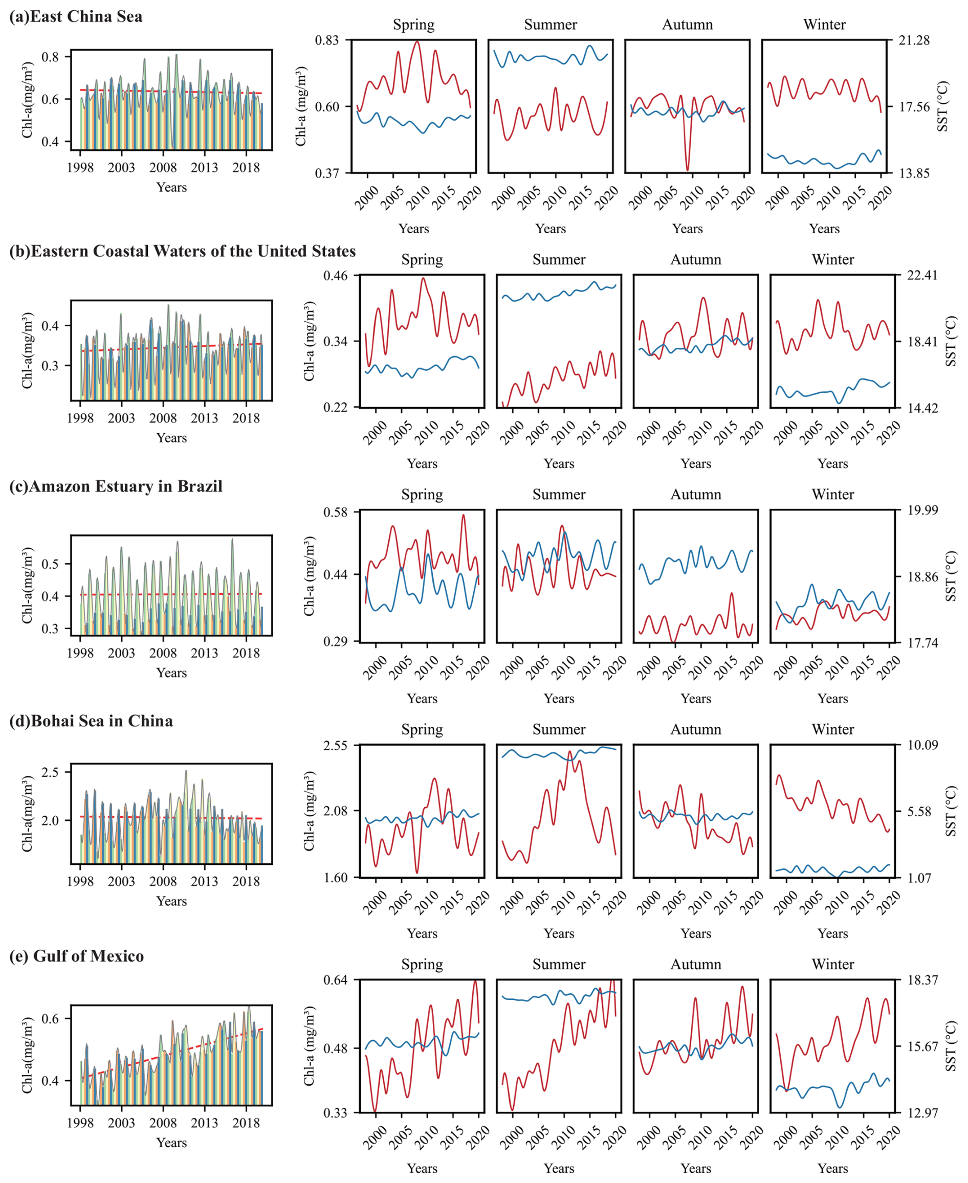
Figure 5 Historical Chl a annual and seasonal variation for the five study areas from 1998 to 2020: (a) the East China Sea, (b) the Eastern Coastal Waters of the United States, (c) the Amazon Estuary, (d) the Bohai Sea in China, and (e) the Gulf of Mexico. The red dashed line in the first bar graph represents a regressive trend line. The red and blue curved lines in line graphs represent the variations in seasonal Chl a and SST, respectively.

3.2 Historical Chl a Variation in the Study Regions

The M-K test revealed distinct temporal trends in Chl a concentrations across the five study areas (Fig. 5). Notably, a statistically significant overall increasing trend was suggested in annual and all seasonal Chl a concentrations in the Gulf of Mexico (p < 0.05). We observed a slight increase in Chl a in the Eastern Coastal Waters of the United States, with a rate of 0.0301 $\mathrm{mg}{\mathrm{m}}^{-\mathrm{3}}{\mathrm{a}}^{-\mathrm{1}}$. We did not observe any statistically significant trends (p > 0.05) in the East China Sea, the Eastern Coastal Waters of the United States, the Amazon Estuary, or the Bohai Sea. A distinct continuous increase of Chl a concentration, however, was indicated in the summer in the sea area of the Eastern Coastal Waters of the United States.

Notably, both the Bohai and East China seas exhibited a two-stage change, with a decreasing tendency after a continuously increasing trend; however, the decline of the East China Sea was not significant. The turning point for the Bohai Sea occurred in 2013, which was earlier than that of the East China Sea in 2017.

Table 5 Correlation analysis between the seasonal and annual Chl a concentrations.

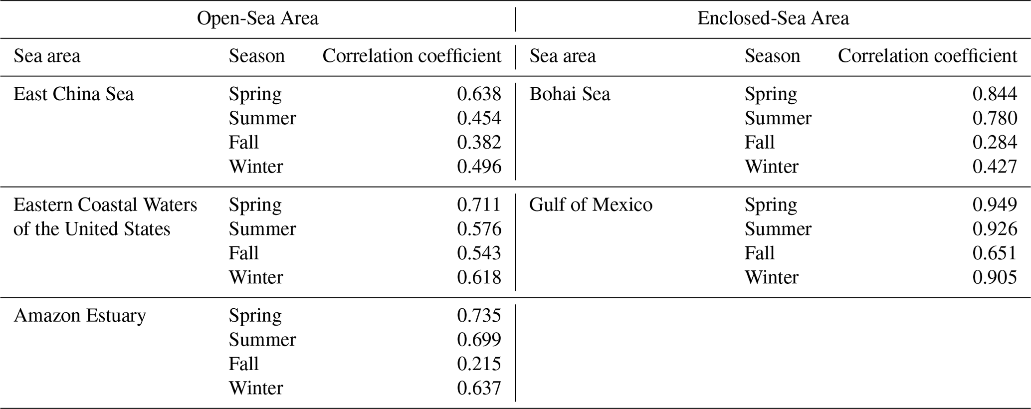
The seasonal mean Chl a concentrations did not always follow the same temporal trend as the annual mean. In the Gulf of Mexico, however, all four seasonal means followed consistent increasing trends that aligned with the annual mean trend (Fig. 5). The correlation analysis between the annual and seasonal Chl a concentrations (Table 5) suggested that the temporal changes in annual Chl a in the Bohai Sea were controlled dominantly by the spring and summer Chl a concentrations. In the Gulf of Mexico, owing to its different hydrodynamic regime, the annual trend was more uniformly correlated across all seasons. In open-sea areas, winter and spring Chl a concentrations were strongly correlated with the annual mean and thus served as the primary drivers of the annual trend. The Amazon Estuary was an exception, and summer and winter Chl a concentrations were more important in determining the annual trend.

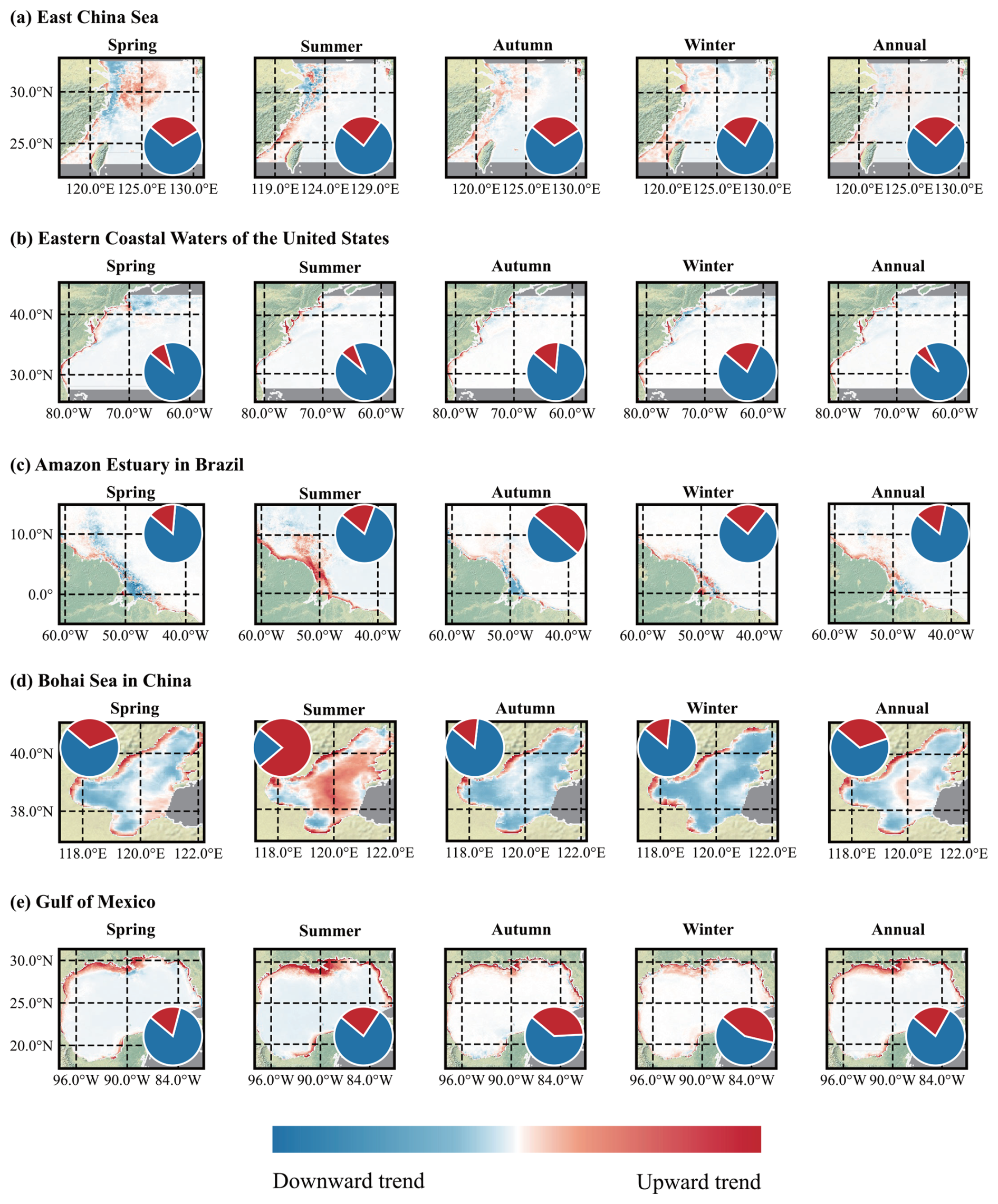
Figure 6 Temporal trends of seasonal and annual Chl a concentrations based on each pixel in the five study areas: (a) the East China Sea, (b) the Eastern Coastal Waters of the United States, (c) the Amazon Estuary, (d) the Bohai Sea, and (e) the Gulf of Mexico. The pie chart shows the proportion of areas with downward (blue) and upward (red) tendencies. The gray–blue areas had no available data.

3.3 Spatiotemporal Variation of Chl a

Figure 6 and Appendix E illustrate the spatiotemporal variation rates of Chl a from 1998 to 2020. Overall, coastal regions exhibited increasing Chl a concentration trends, whereas offshore areas showed declining trends, with the exception of the Bohai Sea (Fig. 6d). The Bohai Sea had the largest area with positive annual growth (33.79 %), whereas the Eastern Coastal Waters of the United States had the smallest area with positive annual growth (6.53 %). Seasonally, the Bohai Sea also exhibited the most extensive increase in Chl a in the summer (Fig. 6d), which contrasted sharply with the Eastern Coastal Waters of the United States, which had the smallest growth area in the summer (8.06 %, Fig. 6b).

While a general decline in Chl a concentration levels was revealed across most time frames in the Bohai Sea, in its central basin in the summer, Chl a concentrations exhibited a sustained increasing trend (Figs. 5d and 6d). This anomaly was likely due to an ecological lag effect of nutrient aggregation in the central basin, which was facilitated by internal hydrodynamical patterns and a weak exchange capability with outer oceanic currents. Such nutrient enrichment in the central basin, particularly under the conditions of elevated summer temperatures, promoted HABs even amid reduced land-based input.

This dynamic, however, was intricately linked to the specific dimensions of the enclosed-sea area and the intensity of human activities within. The Gulf of Mexico, an analogous enclosed marine ecosystem, did not exhibit comparable patterns of Chl a concentration fluctuations. Strong influences from the Gulf Stream and Cuban Current enhanced water exchange with the Atlantic, making its Chl a patterns more akin to those of open seas. In contrast, in open seas, increasing Chl a was primarily confined to coastlines and river plumes, such as the Changjiang Estuary in the spring (Fig. 6a) and the Amazon Plume in the summer (Fig. 6c).

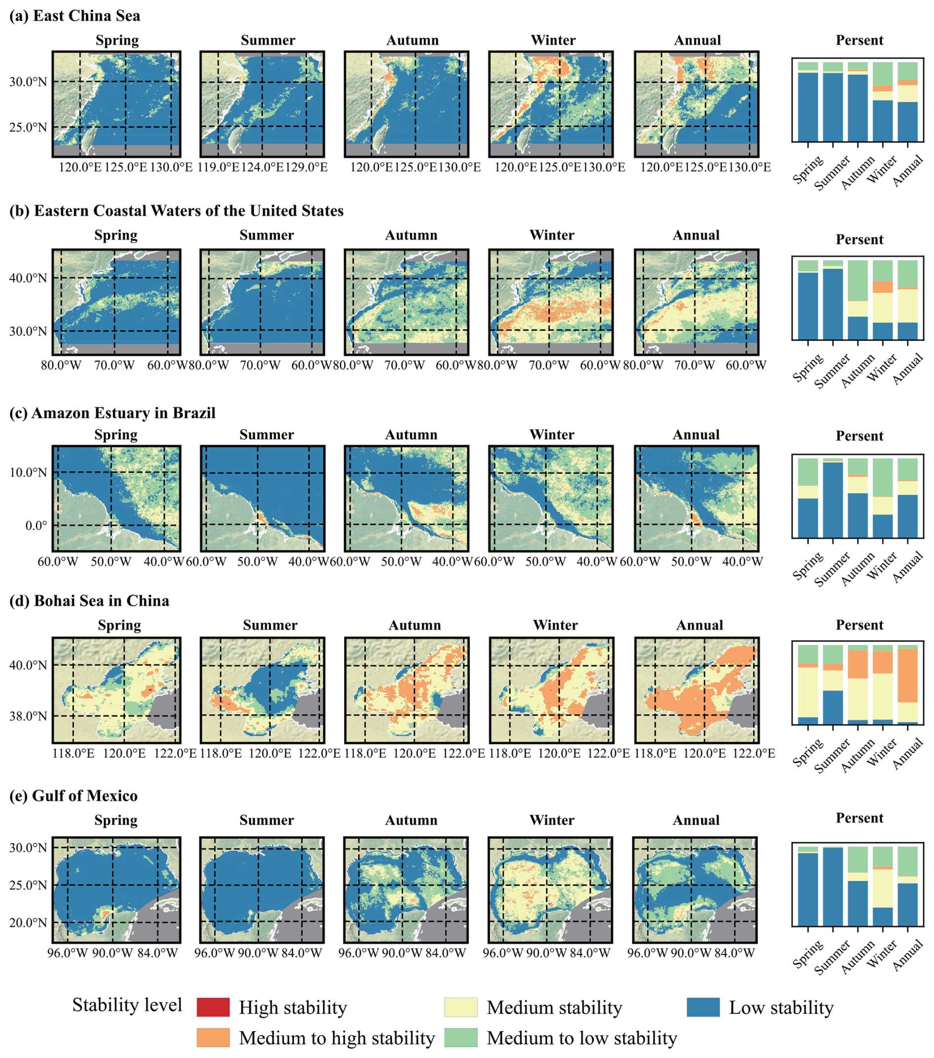
Figure 7 The spatial distribution of the coefficient of variation of seasonal and annual Chl a from 1998 to 2020 in (a) the East China Sea, (b) the Eastern Coastal Waters of the United States, (c) the Amazon Estuary, (d) the Bohai Sea, and (e) the Gulf of Mexico. The percentage bar chart shows the proportion of areas with different stabilities during each season.

3.4 Stability of Chl a

The stability of Chl a, quantified by the coefficient of variation from 1998 to 2020 across the five study regions, is illustrated in Fig. 7 and Appendix F. Regions with obvious increasing or decreasing Chl a trends possessed lower stability. Overall stability varied by sea type. The open seas were less stable than the enclosed seas, and the East China Sea had the lowest stability among all studied waters.

Open seas included the East China Sea, the Eastern Coastal Waters of the United States, and the Amazon Estuary. All the open seas presented unstable Chl a conditions in the spring and the summer. Pronounced seasonal discrepancies in Chl a stability were widely detected in open ocean zones, as shown in Fig. 7a–c. Chl a maintained higher stability in the winter across all study areas. We observed low stability in the Taiwan Strait, Gulf Stream, and Amazon Plume, whereas we observed that Chl a concentrations were relatively steady year-round in the partial waters of the Changjiang Estuary and the area near the mouth of the Amazon River.

Enclosed seas showed distinct stability patterns, represented by the Bohai Sea and the Gulf of Mexico. The Bohai Sea generally maintained moderate-to-high Chl a stability, excluding coastal and estuarine areas. Its stability remained relatively high despite seasonal fluctuations, which differed from the seasonal instability seen in its open-sea counterparts. By comparison, more than 90 % of the Gulf of Mexico featured low or moderately low stability. Areas with intense human activity, such as the northern Gulf and waters around the Florida Peninsula, sustained poor stability throughout the year. We witnessed slightly improved stability in the winter only in the central Gulf, which we attributed to the diminished human interference and decreased SST (Durán-García et al., 2017). Collectively, hydrodynamic conditions and anthropogenic disturbances jointly regulated Chl a stability in both open and enclosed marine environments.

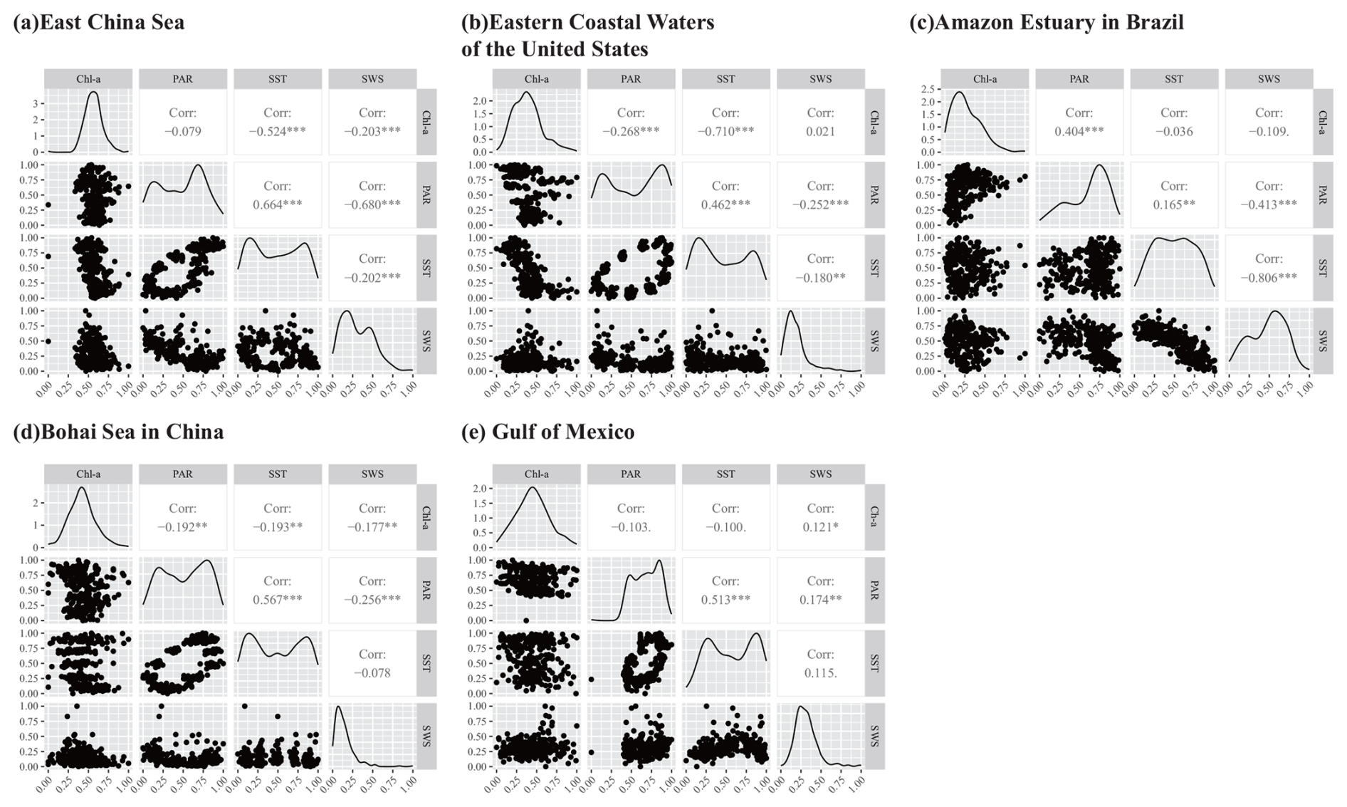
Figure 8 Spatial correlation matrices of Chl a concentrations with environmental factors (SST, PAR, SWS) across the five marginal sea areas: correlation coefficients (r) with significance levels (^∗ p < 0.05, ${}^{\ast \ast }$ p < 0.01, ${}^{\ast \ast \ast }$ p < 0.001) are labeled, and distribution histograms are given for each variable.

4 Discussion

4.1 Factors Affecting Spatiotemporal Changes in Chl a Concentrations

To identify the major environmental factors affecting the observed spatiotemporal changes in Chl a concentrations in the five study areas, we correlated and evaluated the three main environmental indices SST, PAR, and SWS with Chl a using Pearson correlation analysis and PCA (see Sect. 2.3.4). Overall, the correlations between Chl a and the various marine environmental indices varied significantly depending on the study area, as presented in Fig. 8. In comparison with the much stronger correlation between Chl a and SST in the East China Sea and the Eastern Coastal Waters of the United States, and between Chl a and PAR in the Amazon Estuary, we did not identify any evident correlations between Chl a concentrations and the environmental indices in the two enclosed seas. In addition, we did not observe a distinct correlation between Chl a concentrations and SWS in any of the five study areas.

Among the three open seas, trends and degrees of correlations between Chl a and the environmental factors (SST, PAR, and SWS) differed markedly. All three of the open seas showed negative correlations between Chl a and SST. Specifically, the Amazon Estuary demonstrated a weaker negative correlation between Chl a and SST than the East China Sea and the Eastern Coastal Waters of the United States, but it exhibited a significant positive correlation between Chl a and PAR. We observed a stronger negative correlation between Chl a and SWS in the East China Sea, whereas both Eastern Coastal Waters of the United States and the Amazon Estuary exhibited insignificant correlations.

In contrast, in the two enclosed seas, Chl a exhibited only weak or negligible correlations with SST, SWS, and PAR, indicating that environmental factors exerted a comparatively minor influence on Chl a dynamics in these semi-enclosed basins.

Notably, varying degrees of intercorrelations among the three indices were indicated in the five sea areas. Distinct positive correlation between SST and PAR were indicated except in the Amazon Estuary. In addition, various degrees of negative correlation between PAR and SWS were indicated with the correlation coefficient of the East China Sea > the Amazon Estuary > the Eastern Coastal Waters of the United States ≈ the Bohai Sea, whereas the Gulf of Mexico demonstrated weak positive correlation. As for the correlations between SST and SWS, we observed a strong negative correlation only in the Amazon Estuary, whereas the other four sea areas exhibited weakly negative or negative correlations.

Table 6 PCA for the five study locations and three environmental indices. The highest absolute loading for each principal component within each region is shown in bold to highlight the dominant environmental driver.

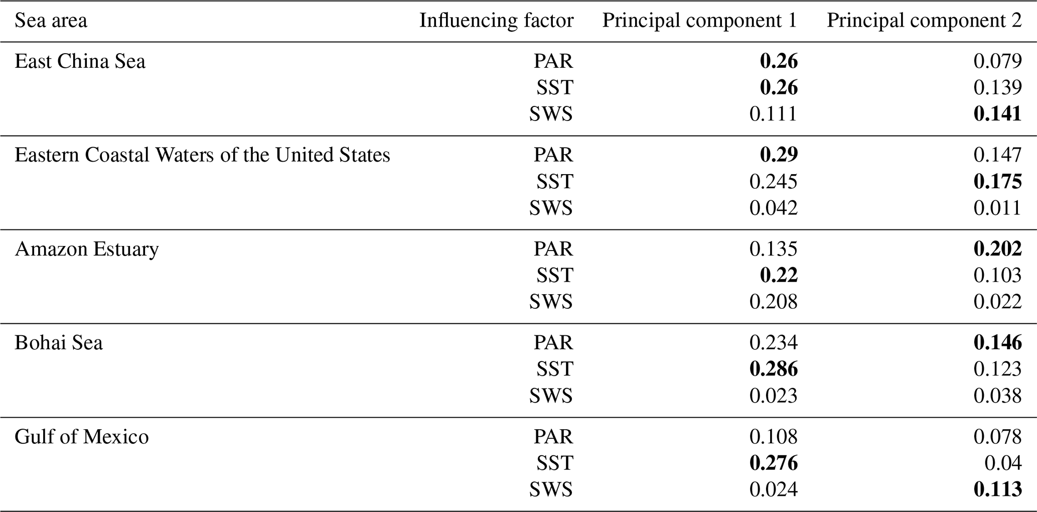
To clarify the key factors dominating Chl a concentration, we conducted PCA for each study area. As shown in Table 6, SST had a relatively high loading on the first principal component across all five sea areas. In the East China Sea, PAR had a loading comparable to SST, whereas in the Eastern Coastal Waters of the United States, PAR showed a higher loading than SST. In the Bohai Sea, PAR had a slightly lower loading than SST, which was much lower than SST in the Gulf of Mexico and the Amazon Estuary.

These results suggested that seasonal SST variation in the Eastern Coastal Waters of the United States, and the Bohai Sea, was closely associated with seasonal PAR variation. In contrast, in the Amazon Estuary, sustained solar irradiance near the equator may have weakened the coupling between SST and PAR, making SST more susceptible to oceanic water intrusion and hydrological processes. In the Gulf of Mexico, SST variation may be strongly influenced by ocean circulation, including the Gulf Stream, explaining the lower PAR loading on the first principal component. SWS showed larger loadings on the first principal component in the three open-sea areas than in the Bohai Sea and the Gulf of Mexico, possibly reflecting wind-driven vertical mixing and nutrient input from deeper waters.

In general, the loading on the first principal component was likely related to seasonal variation of SST, PAR, and SWS. The enclosed-sea areas of the Bohai Sea and the Gulf of Mexico were more susceptible to seasonal SST variation and less susceptible to SWS. For the open-sea areas of the Eastern Coastal Waters of the United States and the East China Sea, both the seasonal variations of SST and PAR have been important in enhancing phytoplankton biomass. In contrast, for the Amazon Estuary of Brazil, which is located at the equator, the guarantee of solar irradiance has made SST independent from PAR, and PAR has less significantly affected Chl a than SST and SWS.

4.2 Key Factors Affecting Chl a Concentrations

The regulation of Chl a concentrations across the five study areas is due to a complex interplay between physical forcing and biogeochemical cycles. The dominant driver has shifted from climatic factors in open oceans to anthropogenic nutrients in enclosed seas.

4.2.1 Natural environmental factors

SST, PAR, and SWS exhibited regional influence on Chl a concentrations. For the open seas, the distinct negative correlations between SST and Chl a in the East China Sea and the Eastern Coastal Waters of the United States indicated the suppressive effect of Chl a by SST when increased in the context of global warming. This result aligned with the paradigm that warming has intensified stratification, thereby limiting the vertical flux of nutrients to the euphotic zone (Behrenfeld et al., 2016). In this context, the influence exerted by seasonally varying SST must be interpreted cautiously. In contrast, the Amazon Estuary has presented a notable anomaly with an insignificant SST–Chl a correlation. This decoupling supports the hypothesis that SST in this region was primarily a passive tracer of low-salinity plume intrusions rather than a direct biological driver. The formation of a near-surface barrier layer inhibited mixing and elevated SST independently of atmospheric heating (Balaguru et al., 2012; Coles et al., 2013; Ferry and Reverdin, 2004; Grodsky et al., 2012). These results explained why PAR, rather than SST, has governed local phytoplankton dynamics in this region (Foltz and McPhaden, 2009; Gomes et al., 2018). Similar to SST, the effect of PAR on Chl a has also been diverse. High turbidity may have reduced the solar radiation available to phytoplankton and led to regionally low biomass, such as in the Hangzhou Bay, in the northern Changjiang Estuary of the East China Sea. In addition, open-sea areas experience greater sensitivity to SWS compared with the enclosed seas. SWS is closely related to current and upwelling activity, which have profound impacts on Chl a concentration. Several regions influenced by ocean circulation have exhibited unstable Chl a concentration due to upwelling of deeper seawater with suitable SST, salinity, and nutrients for phytoplankton growth (Figs. 6 and 7).

SST, SWS, and PAR sensitivity was found to be significantly different in enclosed systems. The very weak correlations between Chl a and SST, PAR, and SWS indicated that these natural environmental factors have had an insignificant impact on long-term Chl a change. The stability of the regions where large ocean currents interact with seawater (such as the sea area near the Bohai Strait and in the Gulf Stream active area) is consistently low throughout the year (Figs. 6 and 7), suggesting that oceanic currents are a critical factor in enclosed seas that are closely intertwined with marine environmental indices, such as SST and SWS. In addition, enclosed-sea areas present a more complex seasonal pattern of Chl a distribution. In particular, the Bohai Sea exhibited complex seasonal patterns in which physical factors have often been overridden by local retention and biological consumption, such as zooplankton grazing, leading to late-summer Chl a minima (Duan et al., 2020; Ministry of Water Resources, PRC, 2021).

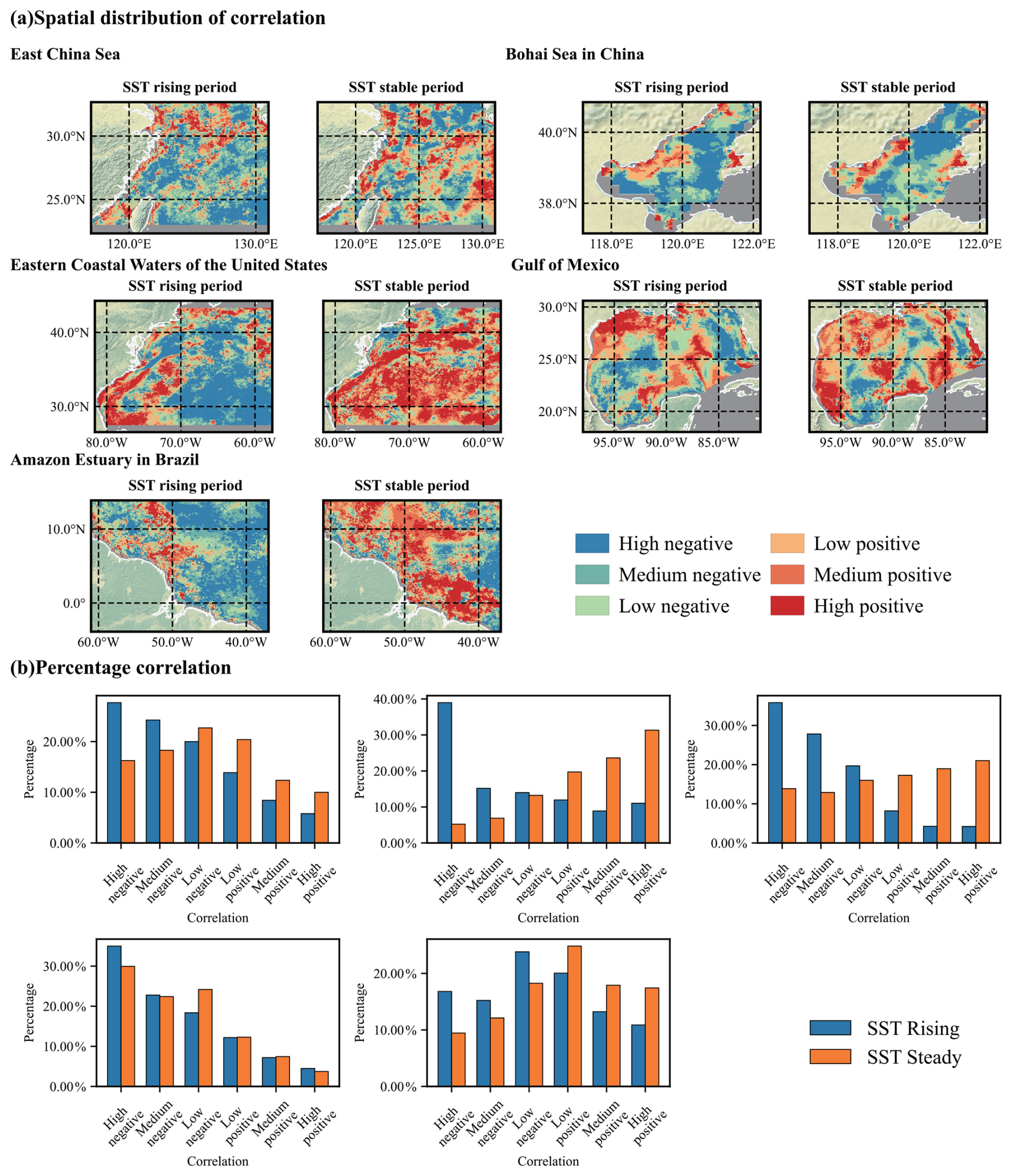
Figure 9 Spatial distribution and correlation proportion between SST and Chl a in five marginal seas, 1998–2020. (a) Spatial patterns of Pearson correlation coefficients in rising and stable SST stages. Color scale: blue = strong negative correlation (−1 to −0.7, Chl a declines with rising SST); green = moderate negative correlation (−0.7 to −0.4); light green = weak negative correlation (−0.4 to 0); light orange = weak positive correlation (0 to 0.4); orange = moderate positive correlation (0.4 to 0.7); red = strong positive correlation (0.7 to 1.0, Chl a rises with increasing SST). (b) Proportional distribution of correlation magnitudes in different sea regions during rising (blue bars) and stable (orange bars) SST periods.

4.2.2 Warming effects on Chl a under regional thermal variability

To isolate the impact of global warming from seasonal cycles, we compared the relationship between SST and Chl a during periods of rising and stable SST in the five study areas (Fig. 9). Compared with the enclosed-sea areas, the open-sea areas were more significantly affected by SST variations. The proportion of correlations during rising and stable SST periods exhibited distinctly opposite distribution patterns. For example, during rises in SST, the areas with negative correlations increased significantly in the East China Sea, reaching 71.92 % of the total. In the Eastern Coastal Waters of the United States, a similar increase occurred to 68.15 %. The stronger negative correlations were distributed mainly in the areas with the saline intrusion. Notably, nearshore areas and estuarine plume-influenced regions such as the Changjiang Estuary (Fig. 9a; the East China Sea) consistently showed positive SST–Chl a correlations regardless of SST changes. This consistent shift toward negative correlations across most regions during warming periods, particularly in offshore areas, coincided with the intrusion of heated, oligotrophic saline waters (e.g., Kuroshio and Gulf Stream intrusions) (Tan and Cai, 2018; Walsh et al., 2005). This mirrored the “ocean desert expansion” that has been observed in subtropical gyres globally (Polovina et al., 2008). In contrast, nearshore regions, regardless of basin type, maintained positive SST–Chl a correlations. We attributed this persistence to the synergistic effect of rising temperatures amplifying the bioavailability of terrestrial nutrient input (Glibert et al., 2014).

Enclosed seas exhibited a similar dichotomy: (1) The central basins of the Bohai Sea and the Gulf of Mexico showed strengthened negative correlations of Chl a and SST with warming, which suggested that warming was associated with lower phytoplankton biomass in these regions, potentially reflecting enhanced water-column stratification and a reduced nutrient supply. (2) Specific regions, such as the Mississippi and Luanhe river mouths and Liaodong Bay, retained positive coupling as a result of continuous nutrient fertilization (Duan et al., 2020; Rabalais et al., 2007). This pattern may have been influenced by the estuarine plume, which provided nutrients and enhanced Chl a in some areas despite the overall negative correlation trend. Nevertheless, although these patterns highlight strong associations, correlation cannot imply direct causation because of the influence of confounding physical and biological factors.

Notably, substantial subregional heterogeneity exists within the broad definitions of open and enclosed seas when generalizing the response of Chl a to warming. For example, the negative SST–Chl a correlations observed in the open East China Sea were not uniform; they were modulated by localized physical processes, such as the Changjiang Dilute Water Plume and coastal upwelling, which have introduced nutrient-rich waters and altered stratification. Similarly, the Gulf of Mexico exhibited complex spatial patterns in which the influence of the Mississippi River Plume contrasted with the oligotrophic conditions of the central basin. These findings have highlighted that although basin-scale geometry is important, intraregional processes have collectively shaped the local magnitude and direction of Chl a responses.

4.2.3 Anthropogenic nutrient input

Anthropogenic nutrient loading represents the primary driver of long-term Chl a trends, particularly in enclosed seas and estuaries in open seas. Moreover, the environmental impacts of nutrients released by human activities may be further exacerbated by upwelling and other ocean currents, active in the coastal and estuarine zones, or in regions with limited water exchange. For example, in the East China Sea, high Chl a concentrations primarily associated with the Changjiang River Plume and the presence of the Taiwan Warm Current have exhibited significant seasonal variation (Dai et al., 2022; Shi et al., 2023), in particular, a moderate increase in winter. Similarly, the Eastern Coastal Waters of the United States have demonstrated a gradient of decreasing Chl a from nearshore to offshore and northwest to southeast, with seasonal peaks in the spring and the winter (Fig. 4f), consistent with coastal bay nutrient dynamics. The Amazon Estuary has also reflected seasonal variability, with high Chl a areas expanding north-eastward in the spring and the summer (Fig. 4c), which is aligned with nutrient inflows from the Amazon River. In the Bohai Sea, high Chl a concentrations have been sustained in regions such as Laizhou Bay and the Liao River Estuary throughout the year, likely because of strong anthropogenic nutrient input under weaker hydrodynamic forces. In contrast, the Gulf of Mexico, although classified as an enclosed sea, has high Chl a zones primarily around the Mississippi River Estuary and Campeche Bay, where anthropogenic discharges and coastal upwelling have played substantial roles (Martínez-López and Zavala-Hidalgo, 2009).

Situated within the rapidly developing economic belts of China, the Bohai Sea and the East China Sea receive massive nutrient influxes. The high Chl a concentrations in the Changjiang Estuary and Laizhou Bay have been consistent with decades of coastal eutrophication as a result of industrial and agricultural runoff (Nixon, 1995; Seitzinger et al., 2010). Notably, the Gulf of Mexico exhibited the highest rate of Chl a increase despite its strong connectivity with the Atlantic Ocean, suggesting that intensifying local anthropogenic pressures can counteract the mitigating effect of high water exchange (Turner et al., 2008).

A critical observation is the recent divergence in trends. Although the Amazon Estuary has faced increasing nutrient influx because of rising fertilizer use in Brazil (Nitrogen fertilizer use, 2026), the Bohai Sea and the East China Sea have shown a deceleration or reversal of Chl a increase post-2014. This result aligned with the reported effectiveness of stringent environmental policies and pollution control measures implemented in China (Li et al., 2024; Paerl et al., 2020). In addition, the Gulf of Mexico has shown the highest rate of Chl a increase, and its relationship with intensifying human activities despite its stronger connection to the Atlantic merits further attention.

Notably, Chl a concentrations in the central basin of the Bohai Sea have shown a continued increase over time and have remained relatively high. In addition, the outer Changjiang Estuary (impacted by the Changjiang River Plume) has shown a significant increase in Chl a, even though Chl a has decreased in the inner Changjiang Estuary. A similar phenomenon was observed in the plume of the Amazon Estuary in Brazil, particularly in the summer (Fig. 6). This pattern was consistent with the possibility that the influence of land-derived nutrient input may progressively extend toward offshore regions. In these estuarine and nearshore systems, phytoplankton biomass trends have corresponded more strongly with the timeline of anthropogenic nutrient input than with trends in rising SST.

Synthesizing these results revealed a hierarchical control mechanism across the five study areas. First, in the tropical, river-dominated systems of the Amazon Estuary, freshwater plumes and light availability have overridden thermal controls. Second, in the temperate enclosed seas of the Bohai Sea and the Gulf of Mexico, the system's response has been a push and pull between terrestrial nutrient loading and warming-induced stratification through promoting or suppressing biomass growth. Third, in the open seas of the East China Sea and the Eastern Coastal Waters of the United States, large-scale physical processes including upwelling and saline intrusion have dominated, although nearshore zones have remained nutrient-sensitive. This regional heterogeneity has underscored that global climate models predict widespread declines in phytoplankton with warming, but such predictions must be re-estimated by local anthropogenic activity strength and basin geometry, as highlighted in recent global syntheses of coastal ecosystems (Cloern et al., 2016; Kavanaugh et al., 2021).

5 Conclusion

In this study, we created a Chl a time-series dataset spanning 1998 to 2020 using monthly products from SeaWiFS/Chl a and MODIS/Chl a L3. We examined the spatial and temporal variability of Chl a in the Bohai Sea, the Gulf of Mexico, the East China Sea, the Eastern Coastal Waters of the United States, and the Amazon Estuary in relation to various degrees of anthropogenic disturbance and global warming, taking into account factors such as SWS, PAR, and other controls. The following conclusions were drawn.

5.1 The Opposing Effects of SST on Chl a

The results of this study revealed two contrasting Chl a responses to rising SST, which appeared to have been mediated by local environmental settings and nutrient availability. Generally, in widespread areas that showed positive correlations between SST and Chl a during stable SST periods (Fig. 9), this correlation appeared to be related to seasonal SST variation. Additional anthropogenic nutrient input combined with the rising SST may have stimulated phytoplankton proliferation, leading to increasing Chl a along the coast in all five study areas. Despite the control of pollutant emissions to the Bohai Sea and the East China Sea, we observed a continuous increase in Chl a in the central of the Bohai Sea and the Changjiang River Plume in the East China Sea, although there was reduced Chl a along coasts and estuaries, as shown in Fig. 6.

Meanwhile, a significant inhibitory effect of SST rise on Chl a during typical warming periods was indicated. We observed negative correlations between Chl a and SST in most offshore areas, which was consistent with saline seawater intrusion and the influence of large current systems, such as the Taiwan Warm Current in the East China Sea, the Gulf Stream along the Eastern Coastal Waters of the United States, and the North Brazilian Current in the Amazon Estuary. The negative impacts from rising SST on nutrient supply, however, have been concealed by land-derived nutrient-induced Chl a enhancement, especially in nearshore areas, and in the plumes of estuaries in the East China Sea and the Amazon Estuary. Notably, in the Amazon Estuary, despite a significant increase in Chl a in nearshore areas in 2020 compared with 2018, the overall Chl a concentrations followed a decreasing trend. This has meant that the falling trend in Chl a in the offshore region because of global warming effects may no longer be compensated for by additional anthropogenic nutrient input combined with rising SST in the coastal region and the estuary.

For the enclosed-sea areas, the Gulf of Mexico has exhibited a much lower eutrophication level than the Bohai Sea. Its larger spatial extent and stronger connectivity with the Atlantic Ocean, which has been mediated by the Gulf Stream and Cuban Current, enhanced water mass exchange and amplified warming impacts. Consequently, the Gulf of Mexico behaved more like an open-sea system, displaying significant Chl a declines during SST increases (Fig. 9). These opposing responses have underscored the need to better resolve subregional physical drivers, such as currents and upwelling, that may synergize with warming to shape Chl a trajectories.

5.2 Chl a Variation Tendency under Global Warming and Human Responses

The impact of global warming on Chl a concentrations was evident in all three open-sea areas, namely the Amazon Estuary, the East China Sea, and the Eastern Coastal Waters of the United States. We also observed significant decreases in offshore Chl a levels, strongly supporting a linkage to global warming rather than human activity. If SSTs continue to rise and the contribution of riverine nutrient input continues to decrease as a result of long-term pollution control measures, this ecological effect may extend to nearshore areas. Additionally, in the enclosed-sea area of the Gulf of Mexico with medium eutrophic characteristics, the negative influence of global warming on Chl a has also been identified. Rising SSTs and oceanic currents have led to a marked decline in Chl a, particularly in areas where ocean currents enter the Gulf of Mexico. The negative correlation between SST and Chl a in the central Gulf further supports the detrimental impact of global warming on Chl a levels.

The impacts of rising SSTs under global warming in estuaries and along coastal waters, however, have been less pervasive than those from eutrophication. Eutrophication-induced phytoplankton blooms have been expanding into offshore sea areas, although Chl a levels may decline along the coast because of restrictions on anthropogenic nutrient input. In highly eutrophic confined sea areas, such as the Bohai Sea, Chl a levels appear to have been less impacted by rising SSTs under global warming. Despite a decline in Chl a concentrations in coastal waters of the Bohai Sea, the central basin maintains high levels of Chl a because of anthropogenic nutrient input, which currently masks the potential impact of global warming. This lagging effect may be temporary and subject to future nonlinear threshold responses. In the highly eutrophic open sea of the East China Sea, although there has been a significant decline in the rate of Chl a increase in estuaries and along the coast, Chl a levels in the Changjiang River Plume have continued to rise. This suggests that in sea areas with sufficient nutrients and suitable salinity, rising SST may further stimulate HABs. A similar phenomenon has been observed in the plume of the Amazon Estuary, where the area of high Chl a has expanded. Despite the widespread occurrence of decreasing Chl a offshore, the continuous proliferation of phytoplankton in the plume has compensated for the intrusion of warmer and oligotrophic pelagic waters.

The findings of this study contribute to our understanding of the ecological response of marine environments to both human activity and global warming. By continuously controlling the input of land-derived nutrients, the frequency of HABs can be reduced, but high Chl a levels may persist in estuaries and along the coast over the long term. From a broader perspective, nearshore areas will gradually experience greater impacts on nutrient supply from global warming. This study (1) has demonstrated the complex and spatially variable interactions between primary production, SST, and nutrient input and exchange under the dual pressures of changes in human activity and coastal development combined with global warming; and (2) has highlighted the need for further research on the impact of changing coastal and terrestrial nutrient input, including where these have been reduced because of environmental protection measures, on primary productivity in both enclosed- and open-sea areas. Unresolved physical–biogeochemical feedback, such as warming-driven stratification and deoxygenation, have limited mechanistic interpretations of these trends. Framing future research within the Global Carbon Project, GO₂NE, and marine ecosystem regime shift theory will help determine whether marginal seas are approaching ecological tipping points. Linking such insights to Sustainable Development Goal 14 and the United Nations Ocean Decade will be essential for adaptive coastal management and sustainable blue economy strategies under accelerating global change.

Appendix A: Chl a concentration and PAR fitting equations obtained from SeaWiFS and MODIS satellites for each study area

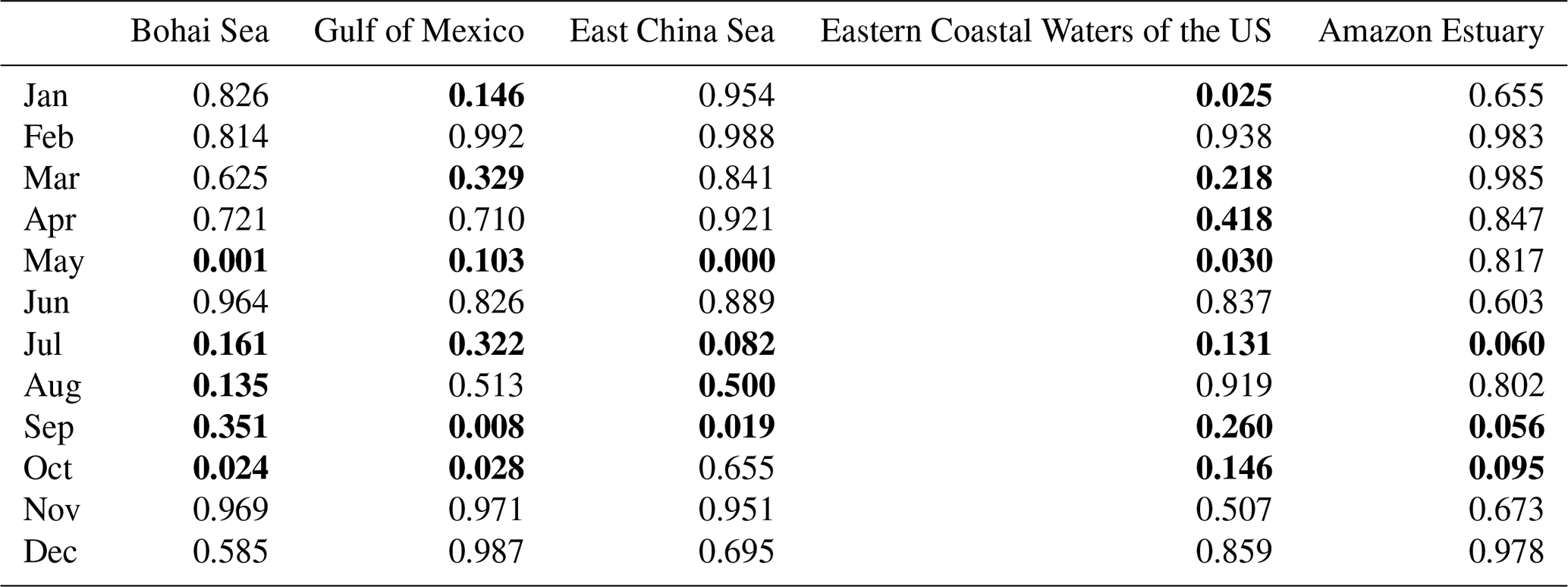
Overlapping Chl a data from MODIS and SeaWiFS during the T2 period were processed with linear regression equations for each month in various sea areas ($y=ax+b$, x, y are the Chl a values of SeaWiFS and MODIS, respectively); and data with R² below 0.5 were not corrected. When R² was greater than 0.5, the equation derived from this linear regression was used to correct SeaWiFS/Chl a. The regression results for each sea area are listed below. The construction methods are shown as follows:

T1 period: corrected SeaWiFS/Chl a values substitute for the original data of corresponding months (Chl a_SWFcorr). For months without correction, the original SeaWiFS/Chl a (Chl a_SWF) are used.

T2 period: Chl a values are calculated through averaging the data from MODIS (Chl a_MOD) and SeaWiFS(${\mathrm{Chl}a}_{\text{SWFcorr}}/{\mathrm{Chl}a}_{\text{SWF}}$).

$$\begin{array}{}\text{(A1)}& {\displaystyle }& {\displaystyle }{\mathrm{Chl}a}_{\text{T2}}=({\mathrm{Chl}a}_{\text{SWF}}+{\mathrm{Chl}a}_{\text{MOD}})/\mathrm{2}\text{(A2)}& {\displaystyle }& {\displaystyle }{\mathrm{Chl}a}_{\text{T2}}=({\mathrm{Chl}a}_{\text{SWFcorr}}+{\mathrm{Chl}a}_{\text{MOD}})/\mathrm{2}\end{array}$$

T3 period: only MODIS/Chl a data are available, Chl a_MOD are used directly.

Based on the threshold of R² > 0.5, the months requiring correction are summarized below.

Months that require correction Chl a concentration in the East China Sea include April, August, September, and December.

$$\begin{array}{ll}{\displaystyle }& {\displaystyle }y=\mathrm{0.661}x+\mathrm{0.251}\\ {\displaystyle }& {\displaystyle }y=\mathrm{0.571}x+\mathrm{0.233}& {\displaystyle }\\ {\displaystyle }& {\displaystyle }y=\mathrm{0.246}x+\mathrm{0.400}\\ {\displaystyle }& {\displaystyle }y=\mathrm{0.439}x+\mathrm{0.323}\end{array}$$

Months that require correction Chl a concentration in the Eastern Coastal Waters of US include April, August, November.

$$\begin{array}{ll}{\displaystyle }& {\displaystyle }y=\mathrm{0.672}x+\mathrm{0.145}\\ {\displaystyle }& {\displaystyle }y=\mathrm{0.835}x+\mathrm{0.086}\\ {\displaystyle }& {\displaystyle }y=\mathrm{1.007}x+\mathrm{0.008}\end{array}$$

Months that require correction Chl a concentration in the Amazon Estuary include June, August, December.

$$\begin{array}{ll}{\displaystyle }& {\displaystyle }y=\mathrm{0.48}x+\mathrm{0.233}\\ {\displaystyle }& {\displaystyle }y=\mathrm{0.519}x+\mathrm{0.198}\\ {\displaystyle }& {\displaystyle }y=\mathrm{0.735}x+\mathrm{0.091}\end{array}$$

Months that require correction Chl a concentration in the Bohai Sea include June, August, December.

$$\begin{array}{ll}{\displaystyle }& {\displaystyle }y=\mathrm{0.851}x+\mathrm{0.424}\\ {\displaystyle }& {\displaystyle }y=\mathrm{1.052}x+\mathrm{0.154}\\ {\displaystyle }& {\displaystyle }y=\mathrm{0.735}x+\mathrm{0.091}\end{array}$$

Months that require correction Chl a concentration in the Gulf of Mexico include March, April, May, June, July, August, November, December.

$$\begin{array}{ll}{\displaystyle }& {\displaystyle }y=\mathrm{0.937}x+\mathrm{0.071}\\ {\displaystyle }& {\displaystyle }y=\mathrm{0.902}x+\mathrm{0.090}\\ {\displaystyle }& {\displaystyle }y=\mathrm{0.758}x+\mathrm{0.132}\\ {\displaystyle }& {\displaystyle }y=\mathrm{0.614}x+\mathrm{0.192}\\ {\displaystyle }& {\displaystyle }y=-\mathrm{0.021}x+\mathrm{0.558}\\ {\displaystyle }& {\displaystyle }y=\mathrm{0.366}x+\mathrm{0.328}\\ {\displaystyle }& {\displaystyle }y=\mathrm{1.139}x+\mathrm{0.009}\\ {\displaystyle }& {\displaystyle }y=\mathrm{1.061}x+\mathrm{0.033}\end{array}$$

Months that require correction PAR data in the East China Sea include January, February, March, April, June, August, October, November, December.

$$\begin{array}{ll}{\displaystyle }& {\displaystyle }y=\mathrm{0.7407}x+\mathrm{3.0500}\\ {\displaystyle }& {\displaystyle }y=\mathrm{0.9062}x+\mathrm{1.2272}\\ {\displaystyle }& {\displaystyle }y=\mathrm{0.6633}x+\mathrm{7.4084}\\ {\displaystyle }& {\displaystyle }y=\mathrm{1.1265}x-\mathrm{4.7338}\\ {\displaystyle }& {\displaystyle }y=\mathrm{0.9306}x+\mathrm{0.3926}\\ {\displaystyle }& {\displaystyle }y=\mathrm{0.5859}x+\mathrm{15.0874}\\ {\displaystyle }& {\displaystyle }y=\mathrm{0.5185}x+\mathrm{12.0817}\\ {\displaystyle }& {\displaystyle }y=\mathrm{0.8109}x+\mathrm{2.7642}\\ {\displaystyle }& {\displaystyle }y=\mathrm{0.4869}x+\mathrm{6.9225}\end{array}$$

Months that require correction PAR data in the Amazon Estuary include January, February, March, April, May, June, August, November, December.

$$\begin{array}{ll}{\displaystyle }& {\displaystyle }y=\mathrm{0.6712}x+\mathrm{9.4768}\\ {\displaystyle }& {\displaystyle }y=\mathrm{1.1324}x-\mathrm{4.8767}\\ {\displaystyle }& {\displaystyle }y=\mathrm{1.1223}x-\mathrm{4.8357}\\ {\displaystyle }& {\displaystyle }y=\mathrm{0.9561}x+\mathrm{1.1267}\\ {\displaystyle }& {\displaystyle }y=\mathrm{0.9114}x+\mathrm{2.4527}\\ {\displaystyle }& {\displaystyle }y=\mathrm{0.6899}x+\mathrm{9.6201}\\ {\displaystyle }& {\displaystyle }y=\mathrm{0.8800}x+\mathrm{4.0144}\\ {\displaystyle }& {\displaystyle }y=\mathrm{0.5721}x+\mathrm{12.6073}\\ {\displaystyle }& {\displaystyle }y=\mathrm{1.1020}x-\mathrm{3.2767}\end{array}$$

Months that require correction PAR data in the Bohai Sea include January, February, March, April, June, November, December.

$$\begin{array}{ll}{\displaystyle }& {\displaystyle }y=\mathrm{1.1750}x-\mathrm{1.8659}\\ {\displaystyle }& {\displaystyle }y=\mathrm{1.2591}x-\mathrm{3.4065}\\ {\displaystyle }& {\displaystyle }y=\mathrm{0.4278}x+\mathrm{8.6293}\\ {\displaystyle }& {\displaystyle }y=\mathrm{0.6687}x+\mathrm{5.9476}\\ {\displaystyle }& {\displaystyle }y=\mathrm{0.9130}x+\mathrm{1.2173}\\ {\displaystyle }& {\displaystyle }y=\mathrm{0.8262}x+\mathrm{1.2522}\\ {\displaystyle }& {\displaystyle }y=\mathrm{0.4056}x+\mathrm{4.1002}\end{array}$$

Months that require correction PAR data in the Gulf of Mexico include January, February, March, April, June, November, December.

$$\begin{array}{ll}{\displaystyle }& {\displaystyle }y=\mathrm{1.0927}x-\mathrm{2.2949}\\ {\displaystyle }& {\displaystyle }y=\mathrm{0.9091}x+\mathrm{2.7284}\\ {\displaystyle }& {\displaystyle }y=\mathrm{1.2825}x-\mathrm{10.5483}\\ {\displaystyle }& {\displaystyle }y=\mathrm{0.3289}x+\mathrm{21.2346}\\ {\displaystyle }& {\displaystyle }y=\mathrm{1.0825}x-\mathrm{1.7048}\\ {\displaystyle }& {\displaystyle }y=\mathrm{1.1187}x-\mathrm{2.0893}\end{array}$$

Table A1 Monthly R² values of Chl-a fitting between SeaWiFS and MODIS for each study area. Bold values indicate R²≤0.5, for which no regression-based correction was applied.

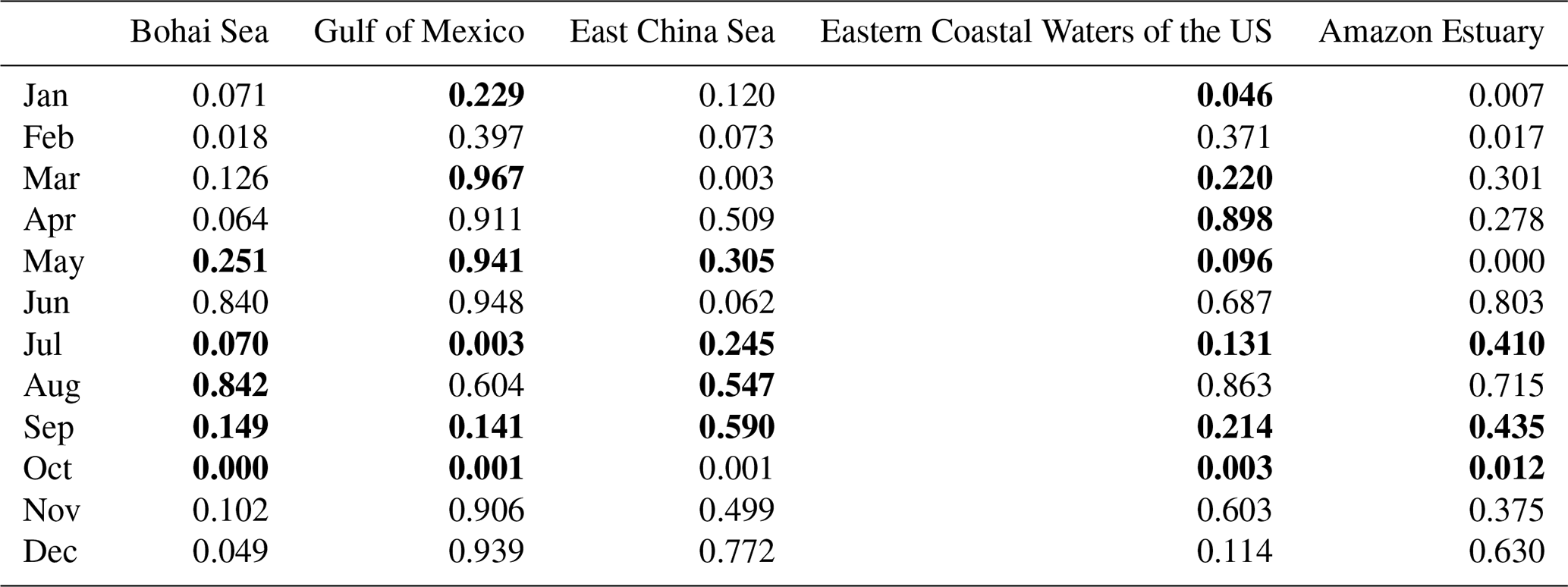
Table A2 Monthly R² values of PAR fitting between SeaWiFS and MODIS for each study area. Bold values indicate R²≤0.5, for which no regression-based correction was applied.

Appendix B: Outlier Removal in Time Series Analysis

To reduce the influence of extreme values on the long-term time-series analysis, an outlier removal procedure was applied before calculating the pixel-level trend and coefficient of variation. For each pixel-level time series, a statistical threshold based on three times the standard deviation was used to identify anomalous values. The method assumes that data points lying far from the mean are relatively rare and may represent abnormal fluctuations.

The criterion for identifying outliers can be expressed as:

$$\begin{array}{}\text{(B1)}& X_{\text{outlier}}\notin [\mathit{\mu }-\mathrm{3}\mathit{\sigma },\mathit{\mu }+\mathrm{3}\mathit{\sigma }]\end{array}$$

where X_outlier represents the outlier values, μ is the mean of the data, and σ is the standard deviation. Data points outside the range $[\mathit{\mu }-\mathrm{3}\mathit{\sigma },\mathit{\mu }+\mathrm{3}\mathit{\sigma }]$ were flagged as outliers and excluded from further analysis.

After outlier removal, the filtered time series was used to calculate the linear trend and coefficient of variation for each pixel. This procedure reduced the potential influence of extreme values on the estimation of temporal trends and variability. In the implemented workflow, the outlier removal was performed once for each pixel-level time series before the final statistical calculations.

Appendix C: Slope Trend Analysis

The annual variation rate slope of Chl a from 1998 to 2020 is calculated using the least squares method. This method determines the linear trend in the data by fitting a straight line through the time series, where the slope represents the average annual rate of change. The slope is calculated using the following formula:

$$\begin{array}{}\text{(C1)}& \mathrm{Slope}={\displaystyle \frac{n\sum _{i=\mathrm{1}}^n\left[i(\mathrm{Chl}a{)}_i\right]-\left(\sum _{i=\mathrm{1}}^{n}i\right)\left(\sum _{i=\mathrm{1}}^n(\mathrm{Chl}a{)}_i\right)}{n\sum _{i=\mathrm{1}}^n{i}^{\mathrm{2}}-{\left(\sum _{i=\mathrm{1}}^{n}i\right)}^{\mathrm{2}}}}.\end{array}$$

This formula minimizes the residual errors between the observed Chl a values and the values predicted by the fitted line, ensuring the most accurate representation of the trend. The slope obtained provides a quantitative measure of the rate of change in Chl a concentration over the period. A positive slope indicates an increasing trend in Chl a concentrations, while a negative slope signifies a decreasing trend.

Appendix D: Stability Analysis

The stability of a time series over time can be evaluated using C_v, which provides a standardized measure of the dispersion of the data relative to its mean. This is particularly useful for understanding the consistency of values in the time series across the observed period. The formula for C_v is expressed as:

$$\begin{array}{}\text{(D1)}& C_{\mathrm{v}}={\displaystyle \frac{\mathrm{1}}{\stackrel{\mathrm{‾}}{x}}}\sqrt{{\displaystyle \frac{\sum _{i=\mathrm{1}}^n(x_i-\stackrel{\mathrm{‾}}{x}{)}^{\mathrm{2}}}{n-\mathrm{1}}}}.\end{array}$$

A lower C_v indicates greater stability in the time series, with less variation relative to the mean, while a higher C_v suggests more significant fluctuations over time.

Appendix E: Areas with increasing or decreasing trend of Chl a from 1998 to 2020

Table E1 Areas with increasing or decreasing trend of Chl a from 1998 to 2020.

Appendix F: Annual and seasonal stability of Chl a in the five locations from 1998–2020

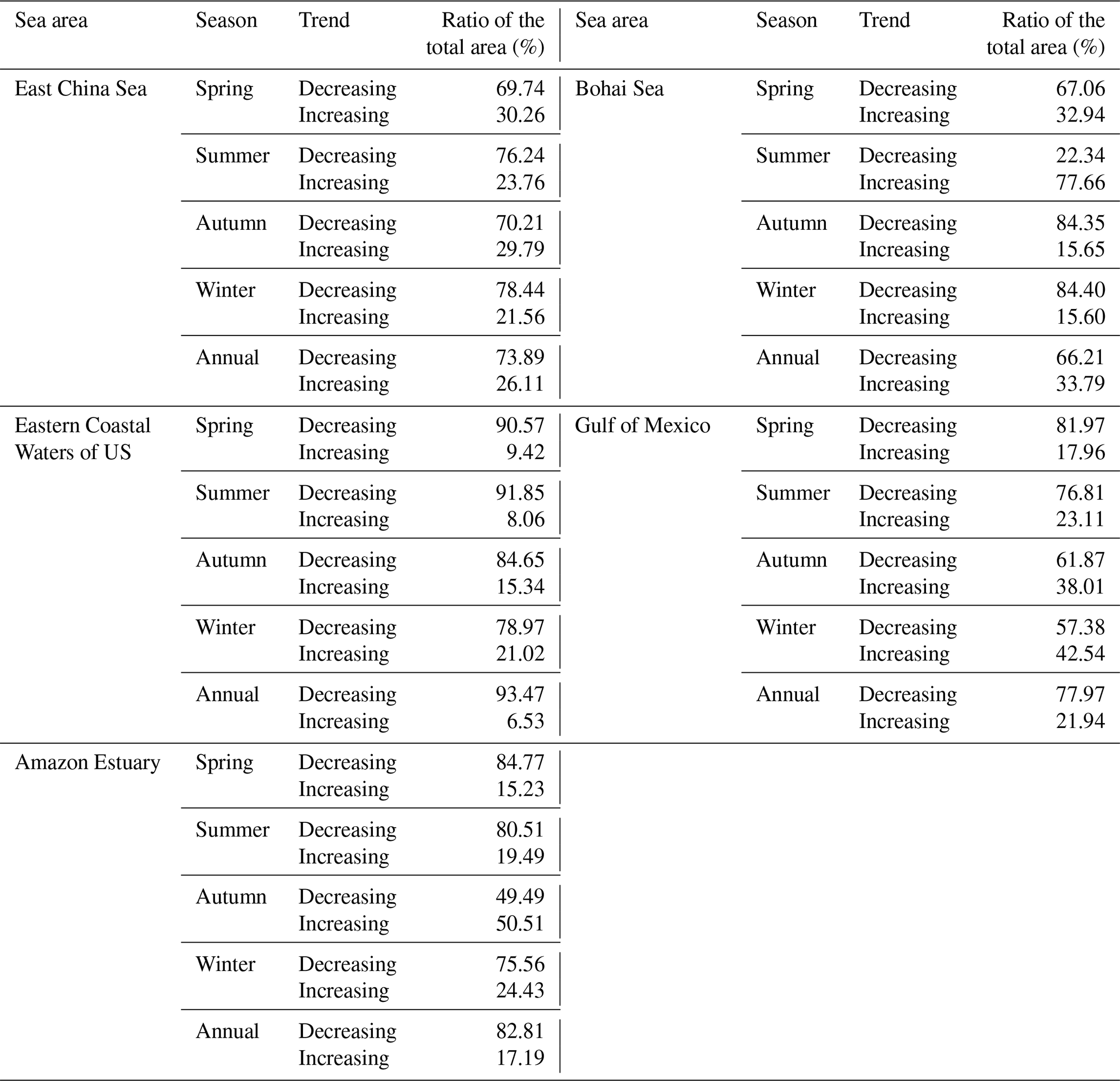
Table F1 Annual and seasonal stability of Chl a in the five locations from 1998–2020.