Evaluate the impact of a 4 h tandem phase on the continuity of nadir altimetry measurements between S3 and S3NG-T

The upcoming Sentinel-3 Next Generation Topography (S3NG-T) mission, designed to succeed the current Sentinel-3 (S3) mission, will operate on the same ground tracks as the current S3 constellation to maximise continuity of measurements, but with a fixed 4 h temporal lag due to satellite design constraints. This configuration prevents the implementation of a classical near-simultaneous tandem phase, traditionally used for inter-mission cross-calibration, and raises concerns regarding the impact of short-term oceanic variability on continuity assessment.

In this study, we evaluate the feasibility and expected performance of a 4 h delayed tandem phase for cross-calibrating S3 and S3NG-T. Using tandem datasets from Sentinel-3A/B and Jason-3/Sentinel-6 missions, combined with SWOT KaRIn observations, we develop a methodology to quantify the oceanic variability introduced by a 4 h delay and to evaluate its effect on the accuracy of inter-mission offset estimates.

Results indicate that the classical tandem configuration achieves regional inter-mission Sea Level Anomaly (SLA) offset uncertainties of approximately 2 mm over a three-month period. In contrast, a 4 h delayed tandem phase increases this uncertainty to about 7 mm in the same period, but still performs significantly better than non-tandem scenarios. Extending the 4 h tandem phase to one year enables the detection of systematic instrumental errors of ±3.5 mm amplitude, sufficient to ensure continuity between S3 and S3NG-T. These findings demonstrate that, despite additional oceanic variability, a 4 h tandem configuration remains a viable and effective strategy for cross-calibration, especially when supported by improved environmental corrections and by extending the observation duration to a full year.

1 Introduction

The Sentinel-3 (S3) and Sentinel-3 Next Generation Topography (S3NG-T) missions are part of the Copernicus Programme led by the European Commission. The European Space Agency (ESA) is mandated to define the Copernicus space component (CSC) architecture based on user requirements coordinated by the Commission, in collaboration with EUMETSAT, and Member States. The S3 and S3NG-T missions aim at providing continuous, high-accuracy measurements of sea surface topography, sea and land surface temperature, and ocean and land surface colour. S3 plays a central role in supporting operational oceanography, environmental monitoring, and long-term climate records. Looking ahead to the 2030–2050 timeframe, the S3NG-T mission's primary objective is to ensure the continuity of the existing Copernicus S3 nadir-altimeter measurements with enhanced performance, coverage and revisit time (European Space Agency, 2025).

The S3NG-T mission consists of two large spacecraft equipped with an across-track interferometer swath altimeter (SAOOH), a synthetic aperture radar (SAR) nadir altimeter (Poseidon-5), a multi-channel microwave radiometer, and a precise orbit determination suite. The two spacecraft will fly in a sun-synchronous orbit at 6 pm local time ascending node (LTAN), at a mean orbital height of 815 km, with an orbital phase difference of 140°, achieving an interleaved ground-track between both satellites, and matching the Sentinel-3A/3B ground tracks. Since S3NG-T satellites will be of a new design, it is imperative that the characteristics of the new system are introduced into the S3 time series in a manner that does not introduce instability into the long time series.

To achieve the primary objective of ensuring the continuity of S3 topographic measurements, it is essential to have a successful cross-calibration between the current S3 constellation and the S3NG-T mission. The most effective method for accurately assessing continuity between successive altimeter missions over the ocean is the tandem flight phase (hereafter referred to as “tandem phase”). During a tandem phase, two successive missions follow an identical ground track separated by a strictly controlled time interval. Tandem phases have been systematically implemented following the launch of new reference altimetry missions, including TOPEX-Poseidon and Jason-1 (2002; 70 s gap), Jason-1 and Jason-2 (2008; 55 s gap), Jason-2 and Jason-3 (2016; 80 s gap), and Jason-3 and Sentinel-6 Michael Freilich (2021–2022; 30 s gap). They have also been used between non-reference missions, such as ERS-2/Envisat (2007–2008, 2010–2011; 30 min gap) and Sentinel-3A and Sentinel-3B (2018; 30 s gap). This S3A/B tandem phase allowed a precise cross-calibration of the S3 constellation instruments (Rieu et al., 2021), supporting the generation of consistent and unbiased time-series observations for climate monitoring (Clerc et al., 2020), following the approach previously applied to the Jason series (Dibarboure et al., 2011). These calibration campaigns are essential for maintaining the accuracy and stability of the satellite altimetry record (Dorandeu et al., 2004; Leuliette et al., 2004; Zawadzki and Ablain, 2016). The significant benefits of a tandem phase have been thoroughly explained by Ablain et al. (2025). A key assumption during this period is that the ocean and atmospheric conditions, at the scales of interest, do not vary significantly between measurements made by the two altimetry missions. This allows for the cancellation of geophysical and atmospheric effects when comparing sea level measurements from the two altimeters. Consequently, the relative errors between altimetry missions, arising from instrumental differences (e.g., altimeter noise), data processing disparities (e.g., retracking algorithms), precise orbit determination, and variations in the mean sea surface, can be accurately determined. Averaging these differences over the entire tandem phase period enables cancellation of random effects, thereby allowing for the accurate determination of systematic instrumental errors between the two successive altimetry missions (Masters et al., 2012; Henry et al., 2014; Guérou et al., 2023).

The precise determination of these systematic sea level differences due to instrumental errors facilitates investigation of their origin and potential future correction. Furthermore, averaging these systematic sea level differences provides the mean sea level offset between two successive missions. This offset is essential for accurately linking the two successive altimeter missions, thereby ensuring a continuous sea level data record.

On the global scale, the mean sea level offset between two successive reference missions is calculated with an uncertainty lower than 0.5 mm at a confidence level of 68 % (Zawadzki and Ablain, 2016; Guérou et al., 2023). At regional scales of a few hundred km, the uncertainty of the mean sea level offset increases to 2 mm (update from Prandi et al., 2021) depending on the area. These uncertainty levels, obtained during the tandem phase, demonstrate our ability to assess the sea level continuity on both global and regional scales between two successive altimetry missions, and represent the limit of detectability of systematic errors.

However, the standard tandem phase with a near-zero temporal lag will not be feasible between S3 and S3NG-T due to orbital constraint, with a 6:00 p.m. LTAN for S3NG-T and 10:00 p.m. LTAN for S3A/B. This configuration imposes a 4 h time lag between the S3 and S3NG-T observations at the same location. As a result, the two altimeters will no longer observe the same oceanic surface simultaneously during their tandem phase. Even when spatially collocated, sea level measurements taken just 4 h apart will differ significantly due to natural, high-frequency ocean processes. These include internal tides, internal waves, inertial motions, mesoscale eddies, and submesoscale dynamics, all of which induce significant fluctuations on sub-daily timescales (Dufau et al., 2016; Cronin et al., 2012). As a consequence, the introduction of ocean variability effects in the sea level differences calculated during a 4 h tandem phase will reduce our ability to assess the sea level continuity between S3 and S3NG-T.

This study aims to evaluate the impact of a 4 h tandem phase on the continuity of sea level measurements provided between S3 and S3NG-T nadir altimetry measurements. To achieve this objective, we explore methods for quantifying the oceanic variability introduced by this 4 h delay and evaluate potential strategies to ensure reliable continuity in the absence of a conventional tandem phase. The datasets used in this study are detailed in Sect. 2. Section 3.1 presents the method used to verify continuity and Sect. 3.2 presents the methodology developed to quantify the associated uncertainty. Section 3.3 describes the approach adopted to characterise the oceanic variability induced by the 4 h lag. The main results are presented in Sect. 4, and additional comparisons with other methods and missions are discussed in Sect. 5.

2 Data

This study relies on altimetric missions with overlapping temporal coverage to evaluate tandem phases and quantify their impact on inter-mission continuity. The primary missions considered include Jason-3 (J3), Sentinel-6 Michael Freilich (S6A), Sentinel-3A (S3A), Sentinel-3B (S3B), and SWOT. These missions provide complementary datasets for different orbits and tandem configurations.

The tandem phase between S3A and S3B serves as a proxy for the future configuration of Sentinel-3D and S3NG-T. This phase represents a relevant case study of two satellites flying on the Sentinel-3 orbit and constitutes the core dataset from which the main results of this study are derived. The S3A/S3B tandem phase lasted from 7 June to 16 October 2018, spanning four complete 27 d cycles or ten 12 d sub-cycles, with a 30 s time interval between the satellites (Clerc et al., 2020).

For comparison, data from the J3 and S6A missions were used to analyse a longer tandem phase on a different orbit, enabling an application of the methodology beyond the Sentinel-3 constellation. The J3/S6A tandem phase extended from 17 December 2020 to 7 April 2022 and includes more than 40 cycles of 10 d, with also a 30 s time interval between the satellites. However, due to an anomaly on the Poseidon-4 altimeter (side A) shortly after the S6A launch, only the data acquired after the switch to side B, performed on 14 September 2021, were retained for this study (Dinardo et al., 2022).

In addition, SWOT KaRIn data were used to estimate the impact of natural oceanic variability on Sea Level Anomaly (SLA) differences over a 4 h time lag. SWOT was selected due to its dense network of dual-crossover points with the S3A and S3B ground tracks, offering high spatial and temporal resolution, which is essential for characterising oceanic variability effects.

The data used in this study are publicly available. We used L2P 2024 products for J3, S6A, S3A and S3B, and the SWOT KaRIn Science Phase data (Version 1.0.2). The SWOT Level-3 Low Rate SSH product, derived from the KaRIn L2 low-rate ocean data, is produced by the AVISO and DUACS teams as part of the DESMOS Science Team project and is freely accessible via AVISO (AVISO/DUACS, 2024).

The L2P contains the along-track SLA at 1 Hz (see Eq. 1) calculated after applying a validation process fully described in the product handbook of each altimetry mission (AVISO+, 2022). The along-track SLA is derived from the following equation:

$$\begin{array}{}\text{(1)}& \mathrm{\text{SLA}}=\text{Orbit}-\text{Range}-{\mathrm{\Sigma }}_i{\text{Correction}}_i-\text{Mean}\text{Sea}\text{Surface}\end{array}$$

where Orbit is the radial distance between the satellite's center of mass and the reference ellipsoid, Range the distance between the satellite and the sea surface, Σ_iCorrection_i are the sum of the geophysical and atmospheric corrections to be applied (e.g. ocean, polar and earth tides, wet and dry troposphere corrections, sea state bias correction,...), Mean Sea Surface is the time-averaged sea surface height referenced to the ellipsoid, from which sea level anomalies are derived. The geophysical corrections applied in L2P products for the SLA calculation are already homogenised for each altimetry mission and identical during a tandem phase.

3 Method

3.1 Comparison between two missions

To evaluate the continuity of sea level measurements between two altimetric missions, we investigate in this study three distinct scenarios. The first is the classical tandem phase, in which the satellites follow each other closely in both space and time, allowing for nearly simultaneous co-located observations. The second scenario considers a configuration without any tandem phase, where sea level data from the two missions are co-located in neither time nor space. The third scenario simulates a delayed tandem phase where measurements are co-located in space but separated by a 4 h time lag. Each of these configurations presents different conditions for estimating the offset between missions, and consequently different associated uncertainties. By comparing the uncertainty in sea level differences across these three scenarios, we aim to assess the feasibility and accuracy of the 4 h tandem phase as a substitute for the classical approach.

We apply a unified processing method to assess measurement continuity across all three scenarios. For each mission, along-track SLA data are aggregated into regular 3° × 3° spatial grids to generate SLA grids. This specific 3° resolution was uniformly selected to minimise empty grid cells and optimise spatial coverage. To ensure a consistent comparison between missions with differing orbital characteristics (e.g., the 10 d cycle of J3/S6A versus the 27 d cycle of S3A/S3B), we adopted a fixed 12 d temporal window for all configurations, corresponding to three 4 d sub-cycles of the S3 orbit. These gridded fields are computed independently for each 12 d period.

From these SLA grids, we calculate the difference between the two missions for each 12 d window, yielding a series of ΔSLA grids. By taking a weighted spatial average of each ΔSLA grid, we obtain a time series of global mean SLA differences between the two missions. The temporal mean of this time series provides an estimate of the global mean SLA offset.

In addition to the global assessment, we evaluate regional SLA offsets to capture geographic variability. Within each grid cell, we extract a time series of the ΔSLA values across the observation period. The temporal mean of these localised time series generates a spatially resolved map of regional SLA offsets. This perspective is critical for analysing geographically dependent phenomena, such as regional instrument biases (Nilsson et al., 2022).

In this study, the focus is placed primarily on regional SLA offset uncertainty. On a global scale, the impact of a 4 h time lag is negligible due to the averaging of uncorrelated oceanic signals. However, at regional scales, such variability can introduce significant errors, making regional analyses crucial to understand the implications of the 4 h tandem configuration.

To clarify the dataset, Table A1 in the Appendix summarises the individual SLA grids and the resulting ΔSLA grids generated across all missions and scenarios.

3.2 Uncertainty computation

Quantifying the uncertainty associated with regional SLA offset estimates is essential for assessing the reliability of continuity verification methods. This uncertainty reflects the variability of differences observed across several repeat cycles and is evaluated separately for each of the three continuity scenarios described above. In this study, we consider two complementary approaches to quantify the uncertainty of regional offset estimates. The first method uses the spatial variance in regional SLA offsets to provide a single global uncertainty value, capturing the overall spread of the regional SLA offset estimates. The second method estimates regional uncertainty at each grid point by analysing the temporal variability of SLA differences between two missions. This approach incorporates the autocorrelation structure of the time series to ensure more realistic uncertainty estimates. These two methods offer distinct yet complementary perspectives – spatial versus temporal – and together provide a more robust and comprehensive assessment of uncertainty under varying observational configurations.

3.2.1 Spatial method

The method described in Sect. 3.1 for comparing missions produces ΔSLA grids for each cycle. The temporal mean of these cycle-by-cycle differences is then computed for each grid cell. This temporal average, $\stackrel{\mathrm{‾}}{\mathrm{\Delta }\text{SLA}}$(lat,lon)${}_{n_{\text{cycle}}}$, represents the regional SLA offset between the two missions over n cycles. This average can be computed during or outside the tandem phase. The uncertainty associated with the regional SLA offset is then quantified as the standard deviation of the spatial variations of this temporal mean. This standard deviation, denoted as

$$\begin{array}{}\text{(2)}& u=\mathit{\sigma }\left(\stackrel{\mathrm{‾}}{\mathrm{\Delta }\text{SLA}}{\text{(lat,lon)}}_{n_{\text{cycle}}}\right)\end{array}$$

provides an estimate of the regional SLA offset uncertainty relative to the global mean. The uncertainty derived from this methodology assumes that the $\stackrel{\mathrm{‾}}{\mathrm{\Delta }\text{SLA}}$(lat,lon) grid represents N independent realisations of the offset error. By verifying that the distribution of these differences follows a Gaussian distribution, the standard deviation can be interpreted as a 1σ uncertainty. To ensure this estimate is realistic, it is crucial to correct for any detectable systematic effects before performing the calculations. Uncorrected systematic errors could inflate the standard deviation, leading to an overestimation of the uncertainty.

3.2.2 Temporal method

Another way to calculate the uncertainty of the regional SLA offset is to compute the standard deviation of each temporal time series of SLA in each grid cell, as proposed by Prandi et al. (2021):

$$\begin{array}{}\text{(3)}& \mathit{\sigma }(\text{lat,lon}{)}_{n_{\text{cycle}}}=\mathit{\sigma }\left(\mathrm{\Delta }{\text{SLA}}_{\text{lat,lon}}\left(t\right)\right)\end{array}$$

The uncertainty for each grid cell is then computed using the formula from Guérou et al. (2023):

$$\begin{array}{}\text{(4)}& u=t_{\mathrm{1}-\mathit{\alpha }/\mathrm{2}}^{n-\mathrm{1}}{\displaystyle \frac{{\mathit{\sigma }}_{\text{lon,lat}}}{\sqrt{n^{\prime }}}}\end{array}$$

and

$$\begin{array}{}\text{(5)}& n^{\prime }={\displaystyle \frac{\mathrm{1}-{\mathit{\rho }}_{\mathrm{1}}}{\mathrm{1}+{\mathit{\rho }}_{\mathrm{1}}}}{n}_{\text{sample}}\end{array}$$

Where σ is the standard deviation of the sample; n is the number of measurements; t is the Student's coefficient for (n−1) degrees of freedom and a confidence level of α; n^′ is the effective sample size, accounting for any autocorrelation in the data.

Unlike the previous approach, which estimates a single regional offset uncertainty relative to the global mean, this method calculates the uncertainty of each local offset. However, for this study, the small sample size during the tandem phase limits the accuracy of n^′.

3.3 Accounting for 4 h variability

To quantify ocean variability and measurement errors over short time intervals, we analysed dual-crossover differences between SWOT’s KaRIn swath data and Sentinel-3A/3B nadir data (ΔSLA). This analysis is based on almost one year of data from SWOT's science phase, leveraging a high number of dual-crossovers and an extensive spatial coverage. A dual-crossover is defined as the intersection of ground tracks from two different satellites, enabling the comparison of spatially colocated measurements, although acquired at different times.

The first step involves constructing a map of ΔSLA variance for dual-crossovers with time interval of Δt=4 h, using data aggregated into 5°×5° grid cells. This map captures high-frequency oceanic variability, systematic errors, and altimeter noise, represented as: ${\mathit{\sigma }}^{\mathrm{2}}={\mathit{\sigma }}^{\mathrm{2}}{}_{\text{ocean}}+{\mathit{\sigma }}_{\text{SWOT}}{}^{\mathrm{2}}+{\mathit{\sigma }}_{\text{S3}}{}^{\mathrm{2}}$ where σ²_ocean accounts for oceanic variability and σ_SWOT², σ_S3² represent the systematic errors and instrumental noise for SWOT and Sentinel-3, respectively.

The second step consists of generating a variance map for Δt approaching 0 h, where the contribution of oceanic variability is negligible. This map isolates systematic errors and altimeter noise in the ΔSLA measurements, providing a baseline against which to compare the 4 h map. Both maps are processed using a mean filter followed by interpolation to fill data gaps and oversampling to a finer 3°×3° resolution. By subtracting the 0 h variance map from the 4 h variance map, an upper bound on the variance associated with 4 h oceanic variability is obtained. This estimate constitutes an upper bound because the calculation may still include residual instrumental and environmental correction errors. The variance associated with altimeter noise is assumed to be time-invariant and therefore cancels out in the subtraction. The resulting variance map is expressed in terms of (σ_i,j²), representing the variance within each 3°×3° grid cell.

This spatial distribution, represented in the left panel of Fig. 1, reveals spatial heterogeneities in the variance of ΔSLA. Notable high values are observed in regions such as the Madagascar Basin, the British Isles and the Indonesian archipelago. These regions are characterised by large tidal amplitudes or complex coastal dynamics. To better understand the origin of this variance, the right panel of Fig. 1 illustrates the evolution of the cumulated variance (σ²) of the ΔSLA at dual-crossover points as a function of the time delay Δt. The systematic errors and instrumental noise for SWOT and Sentinel-3 represented in grey are assumed to be constant over time. The contribution of oceanic variability represented in blue increases rapidly. Specifically, the temporal evolution is not purely linear or random. It exhibits distinct modulations, with a visible signature around 12 h and more pronounced oscillations with a period of approximately 24 h. The correlation between these temporal signatures (diurnal and semi-diurnal) and the coastal areas of high variance observed in the left panel of Fig. 1 indicates that this high-frequency variance is not driven solely by true physical ocean dynamics. It also clearly illustrates the presence of residual errors in the environmental corrections, particularly in tide models.

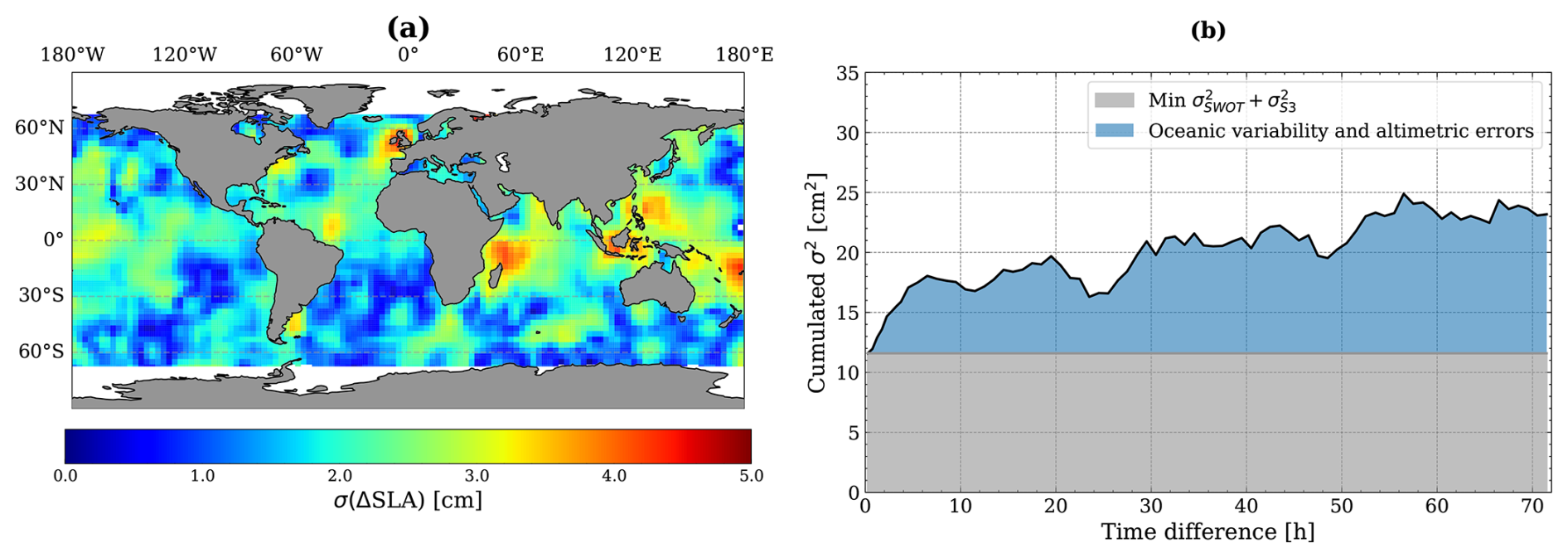
Figure 1 (a) Map of variability in 4 h time interval, from SWOT KaRIn and S3A and S3B dual-crossovers and (b) time series of the cumulated variance of ΔSLA; decomposition between instrumental errors (grey) and oceanic variability (blue).

To simulate the impact of additional sea-level variance due to a 4 h tandem phase, random error grids are introduced into the observed SLA differences during the tandem phase. The 3°×3° grid variance map is used to generate regional random error grids. For each cycle, a random error grid is constructed following a normal distribution with variance σ_i,j². These regional error grids are then added to the ΔSLA grids of S3A and S3B tandem phase. The offset uncertainty is then computed on this new dataset applying the same methodology as described in Sect. 3.2.

This approach was preferred to the use of a global Ocean General Circulation Model (OGCM) or operational model hindcasts, as they struggle to faithfully represent true high-frequency ocean variability. The variability introduced over a short 4 h delay is heavily dominated by high-frequency, sub-daily ocean dynamics, specifically internal gravity waves, internal tides, and sub-mesoscale eddies. While state-of-the-art global ocean models successfully reproduce large-scale mesoscale circulation, accurately resolving the exact global phase and amplitude of these specific high-frequency signals remains a significant modelling challenge. New ultra-high-resolution experimental models, built on the MITgcm framework, are now capable of capturing internal tides and high-frequency sub-mesoscale structures. However, these currently remain advanced research tools rather than standard operational global hindcasts. Therefore, relying on actual recorded satellite altimeter datasets was considered the most appropriate and robust approach to capture the true physical noise floor. Specifically, the SWOT mission resolves kilometer-scale SLA structures across a 120 km swath (Morrow et al., 2019; Archer et al., 2025), enabling a fair representation of the sub-mesoscale structure. For instance, while small-scale waves such as long-crested solitons can be reproduced in ultra-high-resolution models like a 1$/$50° HYCOM simulation, these simulations still under resolve the true abundance and complexity of small-scale features that are directly captured by SWOT (Buijsman et al., 2026).

4 Results

In this section, we compare the continuity performance of three configurations: the classical S3A/S3B tandem phase with a 30 s time interval, a 4 h delayed tandem configuration, and a non-tandem scenario exploiting S3A and S3B data acquired after their tandem phase. The analysis is conducted using along-track comparison methods over a 3°×3° grid with 12 d sub-cycles, as described in Sect. 3.1. The uncertainty presented in these results is computed using the temporal method, which is based on analysing the temporal variability of the ΔSLA grids within each grid cell, as described in Sect. 3.2.2. As shown in Fig. 2, over a period of ten 12 d sub-cycles (approximately four months), the regional inter-mission offset uncertainty is estimated at 2 mm in the classical tandem phase, compared to 7 mm for the 4 h delayed tandem and 10.5 mm in the non-tandem scenario – representing three and five times higher uncertainty, respectively.

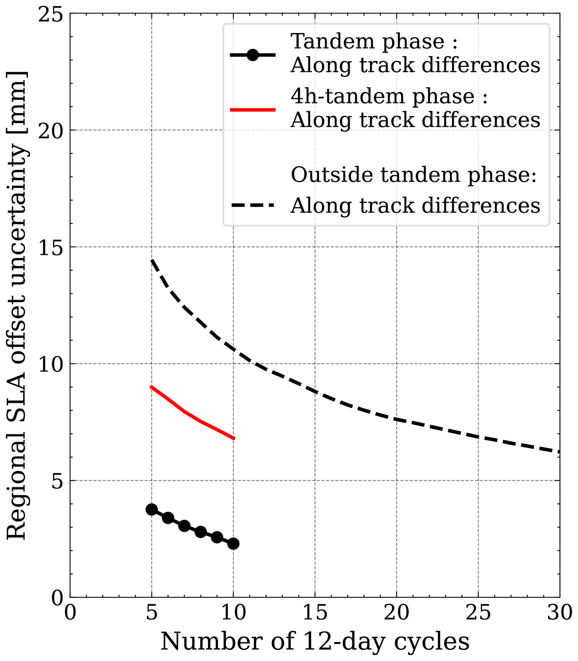
Figure 2 S3A and S3B regional SLA offset uncertainties on 3×3° grid for 12 d subcycles. Uncertainties are computed using the temporal method for three different configurations: classical tandem phase, 4 h tandem phase, and outside tandem phase.

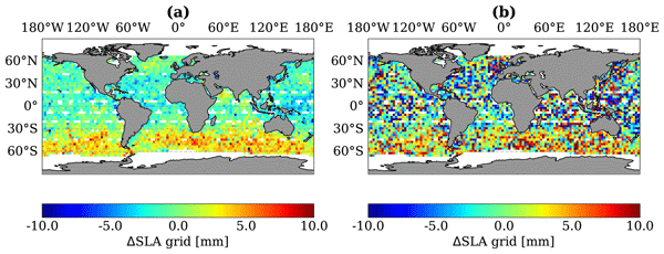
These results underscore the advantage of close spatio-temporal co-location in reducing the measurement noise and improving the inter-mission offset precision. As expected, the uncertainty in the offset estimate decreases with the number of tandem cycles, primarily due to the averaging of random errors. The classical tandem phase enables highly effective detection of systematic differences mainly due to instrumental errors by minimising the effect of differences in oceanic variability. These spatially correlated systematic differences are clearly visible on the regional SLA offset map in panel (a) of Fig. 3. Notably, a distinctive positive offset (up to 7 mm) dominates the high southern latitudes (south of 30° S). This can likely be attributed to differences in how the two altimeters' retracking algorithms process Sea State Bias (SSB), as the Southern Ocean is characterised by high Significant Wave Heights (SWH). These zonal patterns are significantly harder to detect in panel (b), demonstrating how the oceanic variability differences introduced by a 4 h delay masks underlying instrumental errors. In the non-tandem configuration, these same systematic patterns begin to emerge only after one year of observation, with amplitudes reaching up to 6 mm.

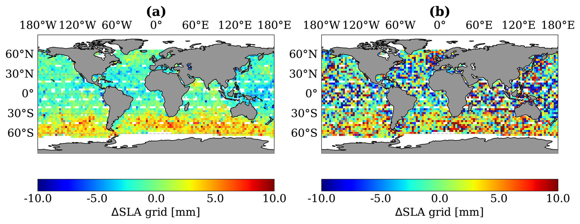
Figure 3 Differences between S3A and S3B for (a) classical tandem phase for 3×3° boxes and (b) 4 h tandem phase for 3×3° boxes.

While the 4 h temporal lag introduces additional variability, the resulting uncertainty remains significantly lower than in the absence of any tandem overlap. This demonstrates that even partial co-location, such as with a few hours of delay, can significantly improve the reliability of continuity assessments.

5 Assessment

This section evaluates the robustness and general applicability of the proposed continuity assessment framework. Specifically, we investigate three complementary aspects: (1) the consistency of results when applied to a different pair of altimetric missions, namely J3 and S6A; (2) the sensitivity of the along-track comparison methodology, evaluated through comparison with a dual-crossover-based approach; and (3) the consistency of regional uncertainty estimates obtained from two distinct statistical methods. Together, these analyses allow us to test the validity, flexibility, and limitations of the proposed methodology under varying mission configurations and observational constraints.

5.1 Comparison with J3/S6A missions

To validate the robustness of our findings, we performed a comparative analysis using J3 and S6A missions (see Fig. 4), which are on a different orbit than S3A and S3B. The uncertainty presented in this comparison is computed using the temporal method described in Sect. 3.2.2. These two missions also benefited from a tandem phase, offering an opportunity to verify the performance observed with the S3A/S3B configuration. Results confirm that orbital characteristics do not significantly affect the ability to detect inter-mission offsets during tandem phases, thereby validating the method across different mission pairs.

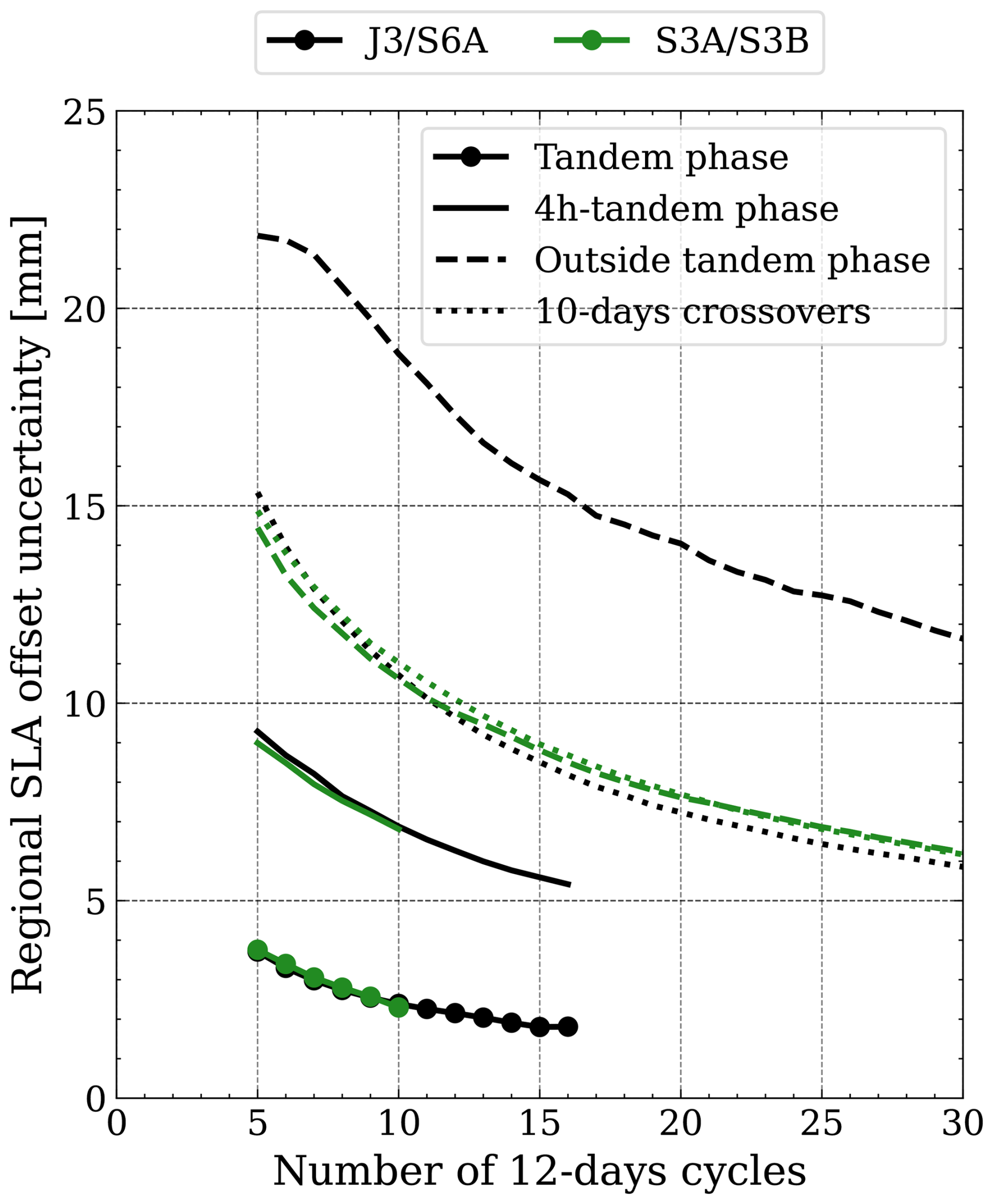
Figure 4 J3/S6A (black) and S3A/S3B (green) regional SLA offset uncertainties on 3×3° grid for 12 d subcycles. Uncertainties are computed using the temporal method for four different comparison configurations: tandem phase, 4 h tandem phase, outside tandem phase and 10 d dual-crossovers.

Outside the tandem phase, however, the orbital configuration becomes a critical factor. After one year of data, the uncertainty ranges from 6 mm for S3A/S3B to 12 mm for J3/S6A. The reference mission orbit (used by TOPEX, the Jason series, and S6A) has a 9.9 d repeat cycle and a ground track separation of 314 km at the equator. In a two-satellite configuration, such as J3 and S6A where J3 is placed on an interleaved orbit following the tandem phase, the inter-track separation at the equator is reduced from 314 to 157 km after one full cycle. For S3A/S3B's configuration, this separation is reduced from 104 to 52 km, reducing the impact of oceanic variability. The offset uncertainty observed in these non-tandem conditions is highly sensitive to such geometric configurations.

Beyond validating the S3A/S3B findings, the extended J3/S6A tandem phase allows us to model the expected reduction in uncertainty over longer operational time frames. Statistically, the uncertainty of a temporal mean decreases proportionally to $\mathrm{1}/\sqrt{n}$, where n is the number of observation cycles. Because both the S3A/S3B and J3/S6A tandem phases share an identical spatial and temporal configuration with a 30 s time delay between satellites, their uncertainty estimates show excellent consistency and follow the same statistical decay behaviour. However, the S3A/S3B tandem phase was relatively short. Therefore, we used the significantly longer J3/S6A tandem phase dataset to achieve a more robust empirical fit for the theoretical $\mathrm{1}/\sqrt{n}$ decay model (Fig. 5, left panel). Relying on this validated baseline, we extrapolated the shorter S3A/S3B 4 h tandem phase uncertainty curve into the future to establish operational requirements. The right panel of Fig. 5 illustrates the required number of days to reach specific target uncertainties. The horizontal thresholds act as visual guides for 1-, 2-, and 3-year mission durations. Using this extrapolation, we estimate that a 4 h tandem phase would require approximately two years to reach the 2 mm precision achieved by a classical tandem phase in three months. However, intersecting the 4 h tandem curve at the 1-year threshold yields an uncertainty of approximately 3.5 mm.

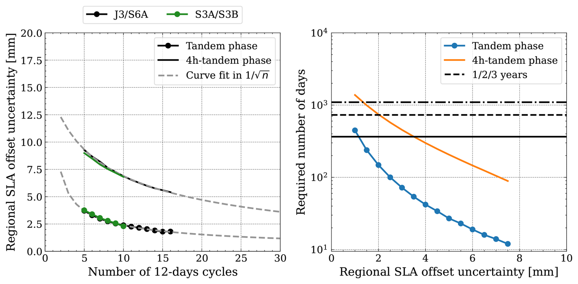
Figure 5 Use of the J3/S6A comparison during the tandem phase to fit the uncertainty evolution (left figure) and to estimate the number of days (right figure) required for the 4 h tandem phase (orange) to reach the same precision as the classical tandem phase (blue). The horizontal black lines indicate, from bottom to top, the 1-, 2-, and 3-year thresholds.

5.2 Comparison with dual-crossover approach

To assess the sensitivity and robustness of the along-track comparison methodology, we conducted a parallel analysis using a second method based on dual-crossovers between the two altimetric missions (see Fig. 4).

The dual-crossover-based method aggregates SLA difference values at these points for time lags below 10 d. This upper limit was chosen to ensure sufficient spatial coverage and data volume for statistically meaningful results. The differences are spatially averaged into 3°×3° grid cells, resulting in gridded SLA difference fields, analogous to those derived from along-track comparisons. The regional SLA offset is then estimated by averaging the time series of each cell across multiple cycles. The associated uncertainty is calculated using the temporal method (described in Sect. 3.2.2), ensuring a homogeneous calculation with the other configurations presented in Fig. 4.

A key advantage of the dual-crossover-based approach lies in its relative independence from the specific orbital configuration or tandem scenario. The method provides consistent results across different mission pairs, such as J3/S6A and S3A/S3B. This robustness to orbital configuration enhances the general applicability of the dual-crossover technique and reinforces its relevance as a complementary method for altimetric continuity assessments. Over a one-year timescale, both configurations yield an uncertainty of approximately 6 mm, closely matching the results obtained outside the tandem phase for S3A/S3B.

5.3 Comparison of two uncertainty estimation methods

To further assess the consistency of uncertainty estimates, we apply both statistical methods described in Sect. 3.2 to a longer tandem phase available with the J3/S6A mission dataset. A comparative summary of the uncertainty evolution derived from both methods is presented in Fig. 6. The primary conclusion drawn from this figure is that both approaches yield highly consistent results, producing nearly identical uncertainty curves as the number of observation cycles increases. This strong agreement cross-validates the two techniques and improves confidence in the overall robustness of our continuity assessment framework. While both methods are valid, they each offer distinct advantages depending on the available data and the specific objectives of the analysis.

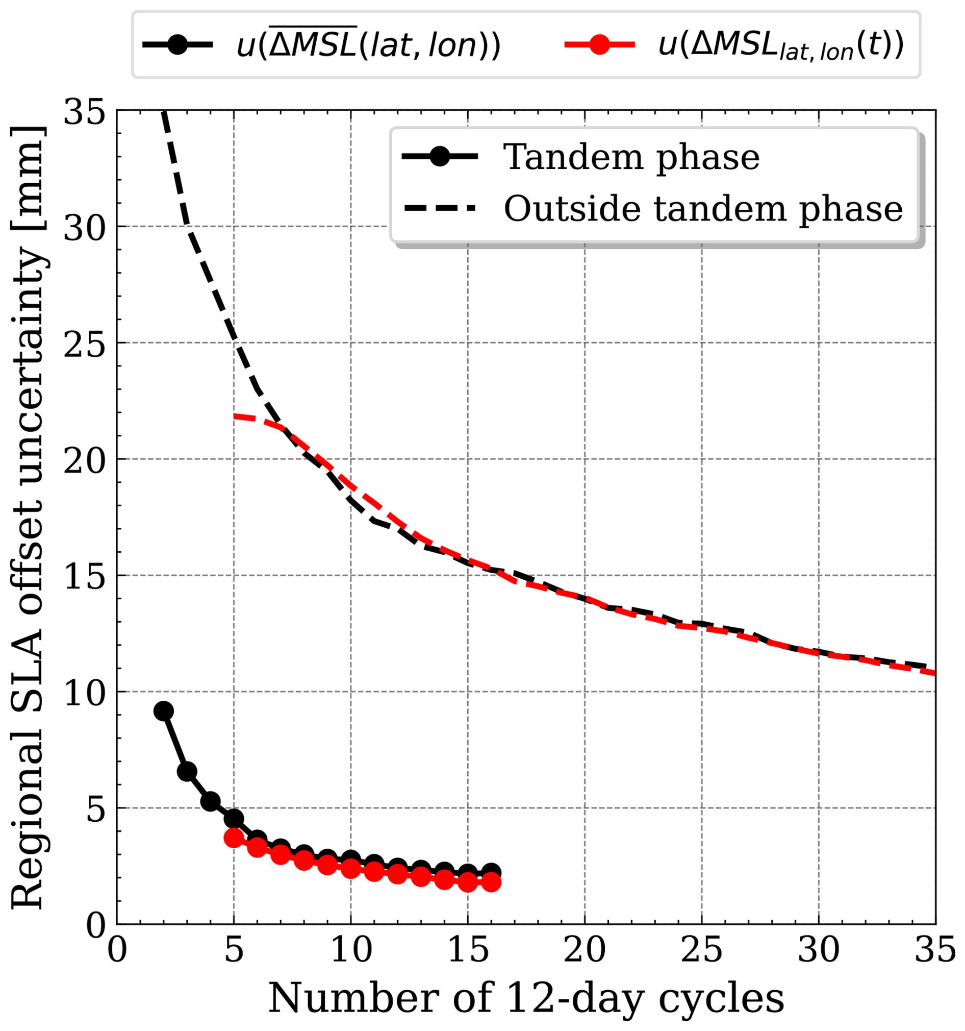
Figure 6 Comparison of two uncertainty estimation methods for J3/S6A in a regional analysis using a 3×3° grid resolution.

The first method, based on the spatial standard deviation of the regional offset field, is particularly well-suited when only a limited number of cycles are available. It allows for a rapid estimation of regional offset uncertainty and serves as an independent validation approach. Its simplicity and minimal data requirements make it especially useful for short-duration tandem phases or initial assessments. It is however sensitive to uncorrected systematic errors that could lead to an overestimation of the uncertainty.

The second method estimates uncertainty at the local scale by analysing the temporal variability of SLA differences within each grid cell. This approach aligns with global uncertainty assessment analyses, ensuring consistency between regional and global uncertainty assessments. One of its major advantages is the ability to produce spatially resolved uncertainty maps, facilitating the construction of detailed regional uncertainty budgets and enabling identification of geographically heterogeneous behaviours. Additionally, this method is less sensitive to systematic error corrections performed beforehand. By explicitly accounting for potential autocorrelation through the calculation of an effective sample size, this approach provides a more rigorous statistical interpretation. However, its reliability is constrained by the number of available cycles, particularly in short tandem phases.

Together, these two complementary uncertainty estimation approaches provide consistent results and improve confidence in the robustness of the continuity assessment framework. However, because the temporal approach is mathematically consistent with the global mean uncertainty assessment, accounts for temporal correlation, and provides geographically resolved insights, we recommend the temporal approach, provided the tandem phase is long enough to supply a sufficient number of observation cycles.

6 Conclusions

This study addresses the critical issue of ensuring continuity in SLA measurements between successive S3 and S3NG-T altimetry missions. Traditional tandem phases, where missions fly in close formation, are crucial for mission continuity. However, orbital constraints prevent a classic tandem phase between S3 and S3NG-T, necessitating a new approach with a 4 h time delay between observations. The introduction of this 4 h delay brings an additional source of uncertainty in offset estimation. Quantifying this uncertainty is essential to evaluate the feasibility and effectiveness of such a configuration for maintaining data continuity. In this study, we developed a technique to simulate the 4 h delay using dual-crossovers with SWOT KaRIn data and assessed its impact by comparing multiple configurations, including scenarios with and without tandem phase, as well as different spatial and temporal sampling schemes. By analysing nearly one year of observations and implementing tailored statistical metrics, we quantified the continuity of SLA measurements between two missions and estimated the associated uncertainties. Beyond the methodological aspects, these findings have significant implications for ocean science and climate applications requiring long-term and stable satellite sea level data records. Our results demonstrate that sea level data continuity between S3 and S3NG-T is maintained despite a 4 h delay instead of a classical near-simultaneous calibration phase. Although this 4 h delay introduces short-term time-correlated effects due to ocean variability, we show that such effects can be effectively quantified and mitigated through an extended calibration period.

Specifically, while classic tandem configurations can achieve a 2 mm detectability threshold within three months, a 4 h tandem phase would require approximately two years of continuous observations to reach a similar level of calibration precision. However, the demonstrated ability to detect systematic differences of ±3.5 mm within one year highlights the feasibility of this approach. Consequently, the methodology developed guarantees to users that future S3NG-T datasets will remain seamless and consistent with the existing S3 legacy, given the possibility of extending the tandem phase to one year.

Although this study focuses on SLA, the methodology is equally applicable to other key altimetric parameters such as significant wave height (SWH) and backscatter coefficient (σ₀). Since the primary objective of S3NG-T is to ensure the continuity of S3 measurements across all topographic products – ocean, inland water (rivers and lakes), sea ice, ice sheets, and atmospheric parameters – the approach developed here holds broad relevance. In addition, the study design supports regional analyses, allowing targeted assessments in specific ocean basins or geographic areas of interest.

A key limitation of the method developed in this study is that SLA differences at a 4 h time lag reflect the combined effects of oceanic variability and altimetric measurement errors. These errors arise from multiple sources, including inaccuracies in environmental corrections such as ocean tides, atmospheric influences, and internal tide signals. Nonetheless, anticipated improvements in altimetric data processing and environmental modelling over the next decade – such as enhanced tide models leveraging SWOT’s high-resolution observations (Zhao, 2024) – are expected to significantly reduce these sources of uncertainty. As a result, future comparisons between S3NG-T and S3 will benefit from these advancements, enabling more precise assessments of mission continuity. An important perspective of this study is then the potential to isolate and quantify the respective contributions of oceanic variability and measurement errors to the overall uncertainty in SLA differences during a 4 h tandem phase. Achieving such a separation would enable a more robust estimation of offset uncertainties and offer valuable insights into the nature and sources of altimetric errors.

Appendix A

Table A1 Summary of the gridded datasets generated for each scenario.