Sea surface salinity downscaling using deep generative diffusion models

High-resolution satellite observations are essential for studying fine-scale ocean processes. Yet, present satellite sea surface salinity (SSS) products remain too coarse to resolve many fine-scale structures. We investigate denoising diffusion models as a generative framework for SSS downscaling in a controlled proof-of-concept experiment based on GLORYS reanalysis fields. A multichannel diffusion prior is trained on $\mathrm{1}/\mathrm{12}\mathit{°}$ SSS, sea surface temperature (SST), and sea surface height (SSH) fields, and is then conditioned at inference time on a synthetically degraded coarse SSS observation ($\mathrm{1}/\mathrm{3}\mathit{°}$) together with high-resolution ($\mathrm{1}/\mathrm{12}\mathit{°}$) auxiliary SST and/or SSH. Conditioning is performed through pseudo-inverse guidance, which steers the generated samples toward states that are compatible with the coarse observation while remaining within the learned GLORYS-consistent multivariate distribution. We also test a gradient-enhancement procedure designed to increase contrast during inference. Experiments in the Gulf Stream region compare models conditioned on SST only, SSH only, and both variables. Validation over the year 2020 uses root-mean-square error (RMSE), structural similarity (SSIM), gradient distributions, and temporal Fourier spectra. In the present GLORYS configuration, conditioning on SST substantially improves accuracy relative to SSH alone; combining SST and SSH yields further gains, comparable to a strong convolutional baseline under RMSE/SSIM, while additionally providing an ensemble of plausible reconstructions. The gradient-enhanced sampler increases structural contrast but can risk amplifying part of the variability, illustrating a trade-off between pixel-wise accuracy and structural realism. Overall, the results support guided diffusion as a promising framework for SSS downscaling and uncertainty-aware reconstruction, while showing that transfer to real satellite SSS products will require product-aware observation operators, uncertainty weighting, and independent in-situ validation.

1 Introduction

Sea surface salinity (SSS) is a fundamental variable for understanding the ocean-climate system. Together with temperature, it controls seawater density and thereby influences thermohaline circulation and the redistribution of heat and carbon. Variations in surface salinity also modulate density stratification of the upper ocean and the solubility of carbon dioxide (CO₂), linking ocean properties and biogeochemical fluxes (Vinogradova et al., 2019; Reul et al., 2020). Accurate high-resolution SSS observations are therefore essential for constraining air-sea exchanges and characterizing freshwater pathways.

Satellite L-band radiometry missions such as ESA's Soil Moisture and Ocean Salinity (SMOS; Kerr et al., 2010), NASA's Aquarius (Lagerloef et al., 2008) and Soil Moisture Active Passive (SMAP; Piepmeier et al., 2017) provide quasi-global SSS coverage with revisit times of a few days, complementing sparse in situ networks such as Argo. However, their effective spatial resolution (typically 40–100 km) remains too coarse to resolve fine-scale processes such as river plumes, sharp frontal gradients, and mesoscale frontal structures that drive upper-ocean variability (Reverdin et al., 2024). Retrieval uncertainties related to surface roughness, sea state, land contamination, rain effects, radio-frequency interference, and auxiliary geophysical corrections introduce errors that are difficult to correct in dynamic coastal and frontal regions (Boutin et al., 2014, 2021), while temporal averaging and filtering further smooth the fields.

To mitigate these limitations, multi-mission and data-fusion products have been developed, combining satellite and model information via optimal interpolation or variational approaches (Olmedo et al., 2016). While these products improve spatio-temporal continuity, they often suppress gradients and small-scale variability. As a consequence, key processes such as eddy dynamics and freshwater advection remain under-resolved, especially in energetic regions such as the Gulf Stream or the Amazon plume (Reul et al., 2020; Reverdin et al., 2024).

Machine learning methods have recently emerged as effective tools to enhance the resolution and quality of oceanographic fields by exploiting nonlinear relationships between variables. Convolutional neural networks (CNNs) have been used to downscale satellite images and reanalysis products, including approaches such as RESAC (Thiria et al., 2023) and related work (Fablet et al., 2021). These approaches are typically deterministic and often produce overly smooth reconstructions, partly because mean-square training objectives favour averaged solutions. They also generally require retraining for each task (e.g. super-resolution, denoising, gap-filling). In this study, RESAC is used as a state-of-the-art baseline.

Diffusion models provide a complementary generative perspective. Originally developed for image generation (Ho et al., 2020; Rombach et al., 2022), diffusion models learn a distribution over high-resolution fields and can generate multiple plausible realizations conditional on observations. This probabilistic formulation naturally represents uncertainty and can better preserve physically plausible variability. Diffusion models are increasingly used in Earth-system science applications such as downscaling, reconstruction, and forecasting (Mardani et al., 2023; Watt and Mansfield, 2024; Tomasi et al., 2025; Finn et al., 2024), highlighting their ability to integrate auxiliary variables and constraints.

Here, we explore denoising diffusion implicit models (DDIM) for downscaling SSS in a controlled setting based on the GLORYS global ocean reanalysis. GLORYS provides complete, collocated gridded SSS, SST, and SSH fields, which allow us to synthetically degrade salinity to a coarse observation while retaining access to a well-defined high-resolution reference for evaluation. Therefore, GLORYS is used here as a controlled gridded reference, not as an error-free truth, and allows us to focus on methodological aspects of the downscaling problem.

Within this framework, we condition the generative process on coarse SSS together with high-resolution auxiliary variables. SST can be coupled to SSS at mesoscale and fine scales represented in GLORYS via mixed-layer dynamics and lateral advection, while SSH encodes mesoscale circulation and front/eddy organization. By conditioning on SST and SSH, we aim to reconstruct the fine-scale frontal and filamentary SSS variability present in the $\mathrm{1}/\mathrm{12}\mathit{°}$ GLORYS reference from degraded observations and to assess what diffusion-based downscaling adds relative to deterministic CNN baselines. The objective is therefore not to generate unresolved fine-scale dynamics absent from the training data, but to recover the structures represented by the high-resolution reference while maintaining consistency with the coarse SSS constraint.

2 Materials

2.1 Study area, data and variables of interest

The study area is located in the North Atlantic Ocean, in the Gulf Stream region (see Fig. 1), bounded to the north and south by 33 and 43° N, and to the west and east by 63 and 52° W, respectively. This sector is characterized by one of the most energetic western boundary currents of the global ocean, with strong jets, meanders and eddies that generate intense temperature and salinity fronts over a wide range of spatial and temporal scales (Chassignet and Xu, 2017; Wu et al., 2022). Such conditions make it an ideal natural laboratory for testing downscaling methods that aim to reconstruct fine-scale structures from coarser information.

Within this domain, SSS, SST and SSH exhibit distinct patterns of spatial variability. As illustrated in Fig. 2, SSS and SST share sharp frontal features and filamentary structures associated with mesoscale and frontal activity. In the present GLORYS-based setup, SSH appears smoother than expected at the fine scale. The close resemblance between SSS and SST gradients suggests that SST is a particularly informative auxiliary variable for constraining the small-scale structure of SSS, whereas SSH primarily encodes the broader mesoscale circulation that organizes the positions and strengths of fronts and eddies.

This leads to the working hypothesis that underpins our modeling strategy: at the mesoscale and at the fine scales represented by GLORYS, SSS variability is tightly coupled to SST through processes such as mixed-layer dynamics and lateral advection, whereas SSH provides a complementary large-scale dynamical constraint. We therefore expect high-resolution SST to provide strong local guidance for reconstructing SSS gradients, with SSH acting as an additional constraint on the overall dynamical context. The diffusion model is designed to exploit these relationships by conditioning the generative process on both variables.

2.2 Data preparation and processing

Our models were trained on GLORYS12V1 CMEMS global ocean reanalysis daily data available at $\mathrm{1}/\mathrm{12}\mathit{°}$ horizontal resolution on 50 vertical levels and produced in the framework of the Copernicus Marine Environment Monitoring Service (Lellouche et al., 2021). In this study, we only use the surface layer. The dataset used in this study consists of daily gridded fields of SSS, SST, and SSH over the Gulf Stream region for the period 1993–2020.

To emulate satellite-based salinity observations, we explicitly distinguish between a high-resolution reference field and a coarse-resolution observation field. The native GLORYS SSS at $\mathrm{1}/\mathrm{12}\mathit{°}$ is taken as the reference high-resolution SSS, while a corresponding coarse SSS field at $\mathrm{1}/\mathrm{3}\mathit{°}$ is obtained by applying a 4×4 spatial averaging and subsampling operator. This correction makes the degradation factor consistent with the ratio between $\mathrm{1}/\mathrm{12}$ and $\mathrm{1}/\mathrm{3}\mathit{°}$. The resulting grid spacing of about 35–40 km is intermediate between the effective footprint of present L-band radiometer missions (typically 40–100 km) and the nominal sampling of commonly used Level-4 multi-mission products, and thus provides a useful idealized proxy for current satellite SSS products (Vinogradova et al., 2019; Reul et al., 2020). Only SSS is degraded in this way; SST and SSH are kept at their native $\mathrm{1}/\mathrm{12}\mathit{°}$ resolution and are used as idealized high-resolution auxiliary fields in the controlled experiments. The choice of $\mathrm{1}/\mathrm{3}\mathit{°}$ is not intrinsic to the method: in principle, the same workflow could be applied to another target resolution by adapting the degradation operator.

This idealized treatment of SSS, SST, and SSH should be kept in mind when considering satellite applications. The present SSS/SST/SSH conditioning experiments should therefore be interpreted as controlled tests rather than as direct operational satellite configurations.

Before training, all variables were linearly normalized to zero mean and unit variance over the training period. This normalization places SSS, SST and SSH on comparable numerical scales and stabilizes optimization. During training, square patches of 64×64 pixels (approximately 600 km×600 km) were randomly extracted from the domain and provided to the model (see Fig. 1). Working with patches rather than full-domain images reduces the memory required per training sample and increases the number of training examples, which is critical given the high dimensionality of diffusion models. At the same time, the energetic nature of the Gulf Stream ensures that strong contrasts and eddy structures are frequently present, even within such smaller spatial windows. These patches therefore provide a rich set of examples for learning the multivariate relationships between SSS, SST and SSH that are exploited in the generative downscaling framework. In doing so, our methodology aims to obtain an SSS patch of 64×64 pixels at $\mathrm{1}/\mathrm{12}\mathit{°}$ resolution, independently of any geolocation information within the region of interest.

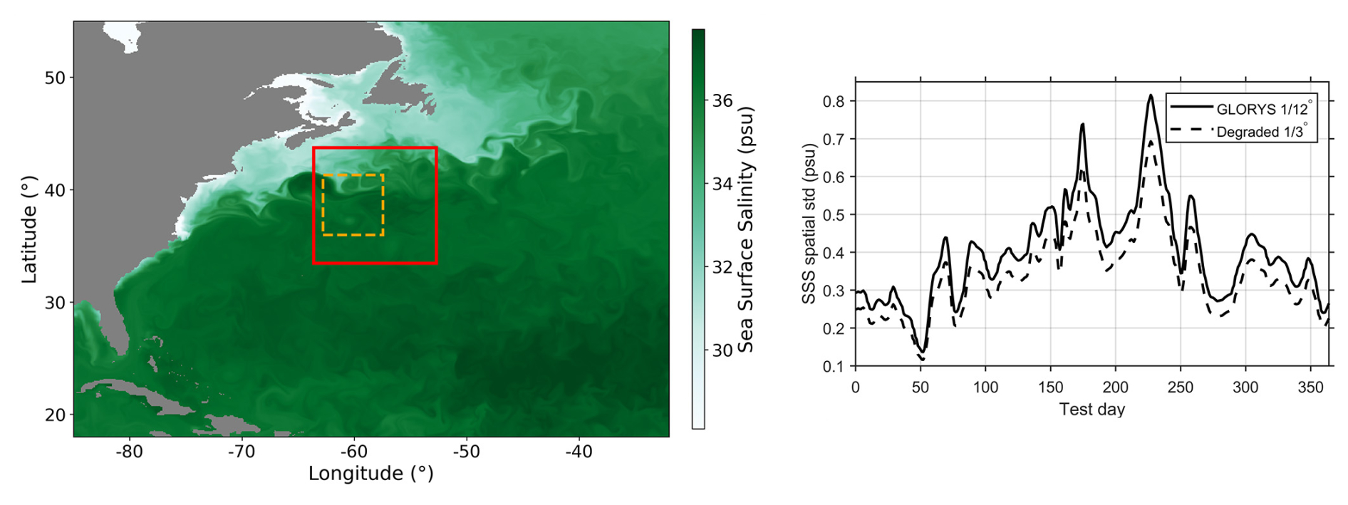
Figure 1 Left: SSS $\mathrm{1}/\mathrm{12}\mathit{°}$ map from GLORYS reanalysis data, in the North Atlantic on 1 January 2021. Our study focuses on the Gulf Stream, in the region highlighted in red. A random 64×64 pixels yellow square inside the red domain indicates the size of patches used during learning phase. Right: daily standard deviation of SSS in the study area for the year 2020.

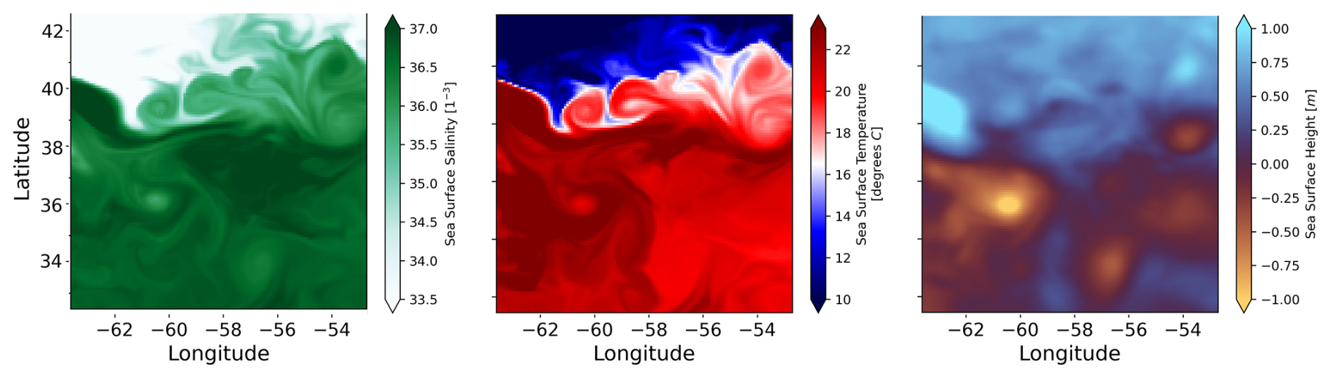
Figure 2 Left to right: Images of SSS, SST, and SSH maps for June 2020 provided by GLORYS for the studied area. SSS and SST present several correlated fine-scale structures, while SSH is much smoother.

3 Method

3.1 The downscaling problem

In this study, downscaling refers to the reconstruction of a high-resolution SSS field from a coarser SSS observation and high-resolution auxiliary variables. We follow the notation commonly used in inverse problems and data assimilation: X denotes the unknown high-resolution state, Y denotes the available observation, and H is the observation operator mapping the state space to the observation space. In the present case, X is the SSS field on the $\mathrm{1}/\mathrm{12}\mathit{°}$ grid and Y is the corresponding coarse SSS observation on the $\mathrm{1}/\mathrm{3}\mathit{°}$ grid. The two are linked by H,

$$\begin{array}{}\text{(1)}& Y=HX+\mathit{\eta },\end{array}$$

where H represents spatial averaging and sub-sampling from $\mathrm{1}/\mathrm{12}\mathit{°}$ to $\mathrm{1}/\mathrm{3}\mathit{°}$, and η is an observation noise term. In our experiments based on GLORYS, Y is synthetically generated from X by applying H.

In addition to the coarse SSS Y, we assume that high-resolution auxiliary variables $Z=(\mathrm{SST},\mathrm{SSH})$ are available on the same $\mathrm{1}/\mathrm{12}\mathit{°}$ grid as X. They can be used alone or together to help estimate the high-resolution state X. These fields share many of the fronts and filaments present in SSS and provide information on the underlying dynamics. From a learning perspective, the downscaling problem consists in estimating a mapping:

$$\begin{array}{}\text{(2)}& \widehat{X}=f_{\mathit{\theta }}(Y,Z),\end{array}$$

parametrized by the model weights θ, such that the prediction $\widehat{X}$ is a high-resolution SSS field on the $\mathrm{1}/\mathrm{12}\mathit{°}$ grid, consistent with Y through the observation operator H and statistically similar to the reference high-resolution SSS fields. Thus, X and $\widehat{X}$ are always defined on the high-resolution grid, whereas Y is defined on the coarse observation grid. In the next subsection, we describe the diffusion-based generative model used to implement this mapping.

The backbone of our diffusion model is a U-Net architecture, widely used in image generation and reconstruction tasks (Ronneberger et al., 2015; Ho et al., 2020; Nichol and Dhariwal, 2021; Rombach et al., 2022). It follows the usual encoder-decoder structure: a sequence of convolutional and attention blocks gradually reduces the spatial resolution while increasing the number of feature channels, then a symmetric decoding path progressively upsamples the representation back to the original $\mathrm{1}/\mathrm{12}\mathit{°}$ grid. In practice, we use a multi-channel U-Net that takes as input the stacked SSS, SST and SSH fields (when available) together with a sinusoidal time embedding of the diffusion step, as in standard DDIM implementations (Ho et al., 2020; Nichol and Dhariwal, 2021). Self-attention layers are included at the coarsest resolutions to capture long-range spatial dependencies, while convolutional residual blocks handle local interactions. Skip connections link encoder and decoder blocks at matching scales, allowing the network to combine local fine-scale information with broader contextual features and to better preserve sharp fronts and filaments (details about the architecture in Appendix A). This design provides a good balance between expressiveness and computational cost for high-resolution oceanographic images.

We present hereinafter the two phases of the classical diffusion model and we propose a new algorithm, the Gradient-Enhancing (GE) algorithm that allows to increase the contrast in the generated SSS $\mathrm{1}/\mathrm{12}\mathit{°}$ samples.

3.2 Learning phase

Diffusion models are a class of probabilistic generative models that learn the probability distribution of a set of training samples in order to generate new, statistically consistent realizations (Ho et al., 2020). In our case, a training sample x₀ corresponds to a high-resolution image on the $\mathrm{1}/\mathrm{12}\mathit{°}$ grid (e.g. including SSS, and in some configurations also SST and SSH channels). Training consists in two phases: a “forward” noising process where gaussian noise is added to the target sample, and a “backward” process where the network learns to gradually remove the noise to retrieve the original sample.

In the forward diffusion process, Gaussian noise is therefore progressively added to an image x₀ over a fixed number T of steps (typically T=1000). At each step t, a coefficient ${\mathit{\alpha }}_t\in (\mathrm{0},\mathrm{1})$ controls the variance of the added noise. After sufficiently many steps, the original information is effectively lost and the sample becomes close to pure isotropic Gaussian noise. The forward process can be written in closed form as

$$\begin{array}{}\text{(3)}& x_t=\sqrt{{\overline{\mathit{\alpha }}}_t}{x}_{\mathrm{0}}+\sqrt{\mathrm{1}-{\overline{\mathit{\alpha }}}_t}\mathit{ϵ},\mathit{ϵ}\sim \mathcal{N}(\mathrm{0},I),\end{array}$$

where ${\overline{\mathit{\alpha }}}_t={\prod }_{s=\mathrm{1}}^t{\mathit{\alpha }}_s$ is the cumulative product of the noise schedule. This formulation allows x_t to be sampled directly from x₀ without explicitly simulating all intermediate steps.

The model then learns to reverse this process during the denoising phase, recovering x₀ step by step by predicting (and removing) the noise ϵ added at each step. In the ϵ-prediction formulation (Ho et al., 2020), the reverse dynamics can be written as

$$\begin{array}{}\text{(4)}& x_{t-\mathrm{1}}={\displaystyle \frac{\mathrm{1}}{\sqrt{{\mathit{\alpha }}_t}}}\left(x_t-{\displaystyle \frac{\mathrm{1}-{\mathit{\alpha }}_t}{\sqrt{\mathrm{1}-{\overline{\mathit{\alpha }}}_t}}}{\mathit{ϵ}}_{\mathit{\theta }}(x_t,t)\right)+{\mathit{\sigma }}_t\mathit{ϵ},\end{array}$$

where $\mathit{ϵ}\sim \mathcal{N}(\mathrm{0},I)$ is fresh Gaussian noise injected to maintain stochasticity in the reverse process, σ_t controls its variance, and ϵ_θ(x_t,t) is the neural network prediction of the noise at step t.

The network parameters θ are trained by minimizing the mean-square error between the true noise and its prediction:

$$\begin{array}{}\text{(5)}& {\mathcal{L}}_{\mathit{\theta }}={\mathbb{E}}_{x_{\mathrm{0}},\mathit{ϵ},t}\left[{∥\mathit{ϵ}-{\mathit{ϵ}}_{\mathit{\theta }}(x_t,t)∥}^{\mathrm{2}}\right],\end{array}$$

where t is typically sampled uniformly from $\mathit{\{}\mathrm{1},\mathrm{\dots },T\mathit{\}}$ and x_t is obtained from x₀ using the forward process above. At this stage, the training is unconditional with respect to the coarse observation: the model learns a prior distribution over high-resolution multichannel images drawn from GLORYS, without yet involving the coarse SSS observations Y or the observation operator H. This prior represents the joint GLORYS distribution of SSS with SST and/or SSH, including their spatial organization and cross-variable relationships. Time is not explicitly modeled in the present architecture but relies on the joint information between SSS and auxiliary variables at the daily situation scale. Extending the framework to a spatio-temporal diffusion model may allow temporal coherence to be learned more directly. Conditioning on (Y,Z) to perform downscaling is introduced at inference time and described in the next subsection.

3.3  Inference phase: Conditioning

Once training is complete, the model is able to generate high-resolution samples that are consistent with the learned joint distribution of SSS, SST and/or SSH as represented in GLORYS. The conditioning on a given observation is then performed during inference. Conceptually, the learned diffusion prior plays a role similar to a statistical background, while the coarse SSS observation provides the constraint imposed through the observation operator.

Several conditioning strategies have been proposed in the literature (Song et al., 2023; Chung et al., 2024); here we follow the pseudo-inverse guidance method of (Song et al., 2023), which offers a good compromise between performance, simplicity and computational cost and can be applied to a wide range of inverse problems beyond super-resolution (see Sect. 5).

We rely on the observation model given in Eq. (1), where X denotes the high-resolution SSS field on the $\mathrm{1}/\mathrm{12}\mathit{°}$ grid, Y the coarse SSS field on the $\mathrm{1}/\mathrm{3}\mathit{°}$ grid, and H the observation operator (spatial averaging and subsampling). We denote by H^† a pseudo-inverse of H that lifts residuals from observation space back to state space (in practice, an upsampling operator from $\mathrm{1}/\mathrm{3}$ to $\mathrm{1}/\mathrm{12}\mathit{°}$).

During inference, let x_t be the current latent state in diffusion step t, and ϵ_θ(x_t,t) the predicted noise. As in the standard ϵ-prediction formulation, we first form a one-step estimate of the clean sample,

$$\begin{array}{}\text{(6)}& {\widehat{X}}_t={\displaystyle \frac{x_t-\sqrt{\mathrm{1}-{\overline{\mathit{\alpha }}}_t}{\mathit{ϵ}}_{\mathit{\theta }}(x_t,t)}{\sqrt{{\overline{\mathit{\alpha }}}_t}}}.\end{array}$$

We then compute the mismatch between this estimate and the observation in the coarse space,

$$\begin{array}{}\text{(7)}& r_t=Y-H{\widehat{X}}_t,\end{array}$$

and project this residual back onto the high-resolution grid using the pseudo-inverse H^†. This defines a guidance term

$$\begin{array}{}\text{(8)}& g_t\propto H^{†}{r}_t=H^{†}(Y-H{\widehat{X}}_t),\end{array}$$

which nudges the reverse diffusion towards the subset of the learned distribution that is compatible with the observations. In practice, g_t is added to the standard reverse update for x_t−1 (see Algorithm A1 in Appendix A for a complete description of the guided inference procedure).

A key advantage of this strategy is that the conditioning is entirely decoupled from the training: the diffusion model is first trained as an unconditional generator on high-resolution GLORYS fields, and different inverse problems (e.g. super-resolution, noisy or masked observations) are handled at inference time simply by changing the operator H and the corresponding pseudo-inverse H^†. Because the reverse process remains stochastic, starting from different realizations of the initial Gaussian noise yields different high-resolution samples that all satisfy the same coarse SSS observation Y, allowing us to explore a range of plausible fine-scale fields instead of a single averaged solution. A schematic representation of the conditional inference phase is shown in Fig. 3.

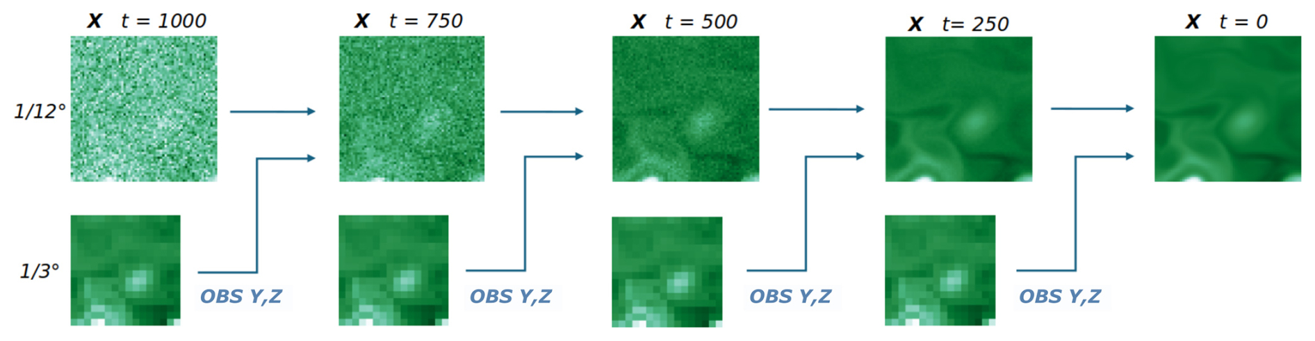
Figure 3 Schematic representation of the conditional inference phase. The first line shows the reverse diffusion trajectory from a random initialization toward a retrieved $\mathrm{1}/\mathrm{12}\mathit{°}$ SSS patch at different steps t. The second line shows the $\mathrm{1}/\mathrm{3}\mathit{°}$ SSS observation used to guide the denoising procedure. For clarity only the coarse SSS constraint is shown, but depending on the configuration the diffusion model generates a multichannel high-resolution state including SSS and the associated SST and/or SSH channels. The evaluated downscaling target remains SSS.

Because the reverse diffusion process remains stochastic, different random initializations give rise to different plausible denoised patches for the same coarse SSS constraint. This raises two related questions: how to select a single displayed reconstruction, and how to interpret the spread across generated samples. In this study, we compute the ensemble mean image and select the generated member that is closest to this mean in ℓ₂ norm. This closest-to-mean member acts as a medoid-like representative of the conditional ensemble: it remains close to the ensemble central tendency while preserving the spatial texture of an individual realization. By contrast, the ensemble mean may reduce pixel-wise error but can smooth fronts and filaments when plausible structures are slightly displaced across members. The choice between an ensemble mean, a representative member, or another criterion is therefore application dependent. The ensemble variance can also be interpreted as a first diagnostic of reconstruction ambiguity.

In the following, we propose the Gradient-Enhancing (GE) algorithm to select the SSS $\mathrm{1}/\mathrm{12}\mathit{°}$ field with the highest contrast, enhancing small structures.

3.4 Gradient-Enhancing algorithm

The image gradient refers to the directional change in the pixel intensity in both the x-axis and the y-axis of an image. It is a key ingredient in image processing and computer vision, particularly in detecting edges or in processing images with edges. The problem of too-low image gradients is common in image reconstruction tasks. Deterministic models optimized with mean-square-error objectives tend to approximate the conditional mean of possible high-resolution solutions, which can smooth fronts and filaments when several plausible fine-scale configurations are compatible with the same coarse observation. During inference, the GE procedure guides the generative process towards higher-contrast samples in the learned distribution. The idea is to favor, at each denoising step, realizations that exhibit stronger local gradients while still remaining consistent with the learned distribution and the coarse SSS constraint. The method is built on top of the pseudo-inverse guidance described above, by adding an additional contrast-based guidance term.

The complete GE algorithm is detailed in Appendix A1 and is applied each time step during the inference phase. In the diffusion timestep t, we consider the one-shot prediction of the network, that is, the current estimate of the final fully denoised image available in DDIM. This estimate gets better and better as the denoising process goes on. On kernels of 2×2 pixels of the image, we enhance the local contrast by subtracting the kernel's mean to the 4 pixels, multiplying by a scaling factor, then adding the mean back. In regions where pixel values deviate strongly from the local kernel mean, indicating the presence of a front or other fine-scale structure, the contrast is amplified. In smoother regions, the effect remains weaker so that no spurious small-scale features are created. The resulting contrast-enhanced image is then fed back into the update for t−1, thereby nudging the network towards higher-contrast samples, which still lie within the learned distribution. The process is sensitive to instabilities, especially for high gradients that can explode over numerous time-steps of multiplicative scaling. The following scaling term provides a damping effect on the highest gradients of the image to prevent those instabilities:

$s=\mathit{\gamma }-\mathit{\delta }\sqrt{{\displaystyle \frac{\left|{\widehat{X}}_t\right|}{max\left|{\widehat{X}}_t\right|}}}$ where max is computed over all kernels.

The scaling factor s is equivalent to γ−δ for high gradients and to γ for small gradients; both parameters are kept close to one and tuned so that the final gradient distribution of the generated images matches as closely as possible that of the test set. In summary, we want to reduce the overall proportion of low gradients, enhance the overall proportion of high gradients, and do so at the right places in the generated samples. In the following, we refer to the diffusion model combined with this gradient-enhancing (GE) procedure as DIFF-SST-SSH-GE.

4 Experiments design

We perform six experiments to understand how diffusion models handle correlated ocean variables and to compare them with a state-of-the-art deterministic approach. The first five experiments use the same diffusion architecture but differ in the auxiliary variables and inference strategy. The first two add either SST or SSH to SSS and are denoted DIFF-SST and DIFF-SSH, respectively. The third is the complete diffusion model conditioned on both SST and SSH, denoted DIFF-SST-SSH. We then apply the GE algorithm during the conditioning phase to enhance the contrast of the generated SSS fields, denoted DIFF-SST-SSH-GE. Finally, we compute an oracle diagnostic, DIFF-SST-SSH-BEST: among multiple samples generated by DIFF-SST-SSH, we select the member closest to the known high-resolution GLORYS reference SSS. This selection requires access to the truth and is therefore not operational; it is used only to estimate the headroom of the generated ensemble. In a last experiment we apply the RESAC methodology adapted to the problem of downscaling of the SSS with the same GLORYS data (SSS and SST). The RESAC model (REconstruction by Scale-Adaptive Convolution) is based on the idea that structures observed in the ocean have approximate fractal properties, and that in incompressible fluids eddies interact most strongly with vortices of comparable size (Thiria et al., 2023). Consequently, two variables are expected to be most strongly correlated at similar spatial scales. These considerations motivated a convolutional (CNN) architecture split into several blocks, in which the resolution of the target variable, in our case SSS, is progressively refined by successively adding SST observations at matching resolutions. The network is thus guided by the scale-dependent physical characteristics of the fields under study, and RESAC provides a strong baseline for assessing the added value of diffusion-based downscaling.

To define our training and testing strategy, the temporal variability of surface salinity must be taken into account. For the Gulf Stream region, the dominant signal is a marked seasonal cycle, with shifts in the position and intensity of fronts and eddies that modulate the distribution of SSS throughout the year, in connection with changes in mixed-layer depth and air–sea fluxes (Chassignet and Xu, 2017). These seasonal shifts are consistent with documented variations in eddy kinetic energy and Gulf Stream path/front dynamics (Zhai et al., 2008; Joyce et al., 2019b, a). We exploit this temporal variability when defining the test configuration. The entire year 2020 is reserved as the independent test set, while the remaining years (1993–2018) are used for training and 2019 for validation and model parameterization. This setup allows us to evaluate not only the reconstruction skill of the diffusion model under typical conditions, but also its ability to generalize across the full seasonal cycle.

In summary, we assess the super-resolution of a coarse $\mathrm{1}/\mathrm{3}\mathit{°}$ SSS observation to a target $\mathrm{1}/\mathrm{12}\mathit{°}$ SSS field, using high-resolution auxiliary SST and/or SSH fields, under the observation model of Eqs. (1) and (2). The domain, period, and preprocessing follow Sect. 2.1. The diffusion prior is trained unconditionally on $\mathrm{1}/\mathrm{12}\mathit{°}$ GLORYS images (Sect. 3.2); observational information is injected at each inference step through the pseudo-inverse guidance of Sect. 3.3. For DIFF-SST-SSH-GE, the gradient-enhancing algorithm (Sect. 3.4) is used. For all diffusion models except DIFF-SST-SSH-BEST, we select the closest-to-mean representative member over 15 samples generated from different random seeds. The main characteristics of the experiments are summarized in Table 1. We note that in diffusion experiments, SST and SSH are treated as generated channels because the diffusion model samples a multichannel ocean surface state. They are not evaluated as final downscaled products in this study; the target variable remains SSS. This formulation keeps a common observation-operator framework for future applications in which SST or SSH may also be partially observed, degraded, or associated with spatially varying uncertainty.

For the deterministic RESAC baseline, RMSE is used as the training loss. For diffusion models, training uses the standard noise-prediction mean-square objective defined in Eq. (5); RMSE between reconstructed and reference SSS is then used as a validation and evaluation metric. Although RMSE is standard in super-resolution and data assimilation applications, it tends to favour overly smoothed solutions that minimize the mean-squared deviation from the reference field. To better assess the quality of small-scale structures, we complement RMSE with three additional indicators: the Structural Similarity Index (SSIM) (Wang et al., 2004), the distribution of spatial gradients, and the temporal Fourier spectrum (FFT) of SSS.

SSIM is widely used in image processing to evaluate the perceptual quality of generated images (Wang et al., 2004; Ledig et al., 2017). It combines luminance, contrast and structural information into a single similarity index, typically between −1 and 1, with 1 indicating locally identical images. Although it has no direct physical meaning for salinity, it provides a convenient way to compare local structures and contrasts between predicted and reference fields. The SSIM between two images x and y is defined locally on a kernel by

$$\begin{array}{}\text{(9)}& \mathrm{SSIM}(x,y)={\displaystyle \frac{(\mathrm{2}{\mathit{\mu }}_x{\mathit{\mu }}_y+C_{\mathrm{1}})(\mathrm{2}{\mathit{\sigma }}_{xy}+C_{\mathrm{2}})}{({\mathit{\mu }}_x^{\mathrm{2}}+{\mathit{\mu }}_y^{\mathrm{2}}+C_{\mathrm{1}})({\mathit{\sigma }}_x^{\mathrm{2}}+{\mathit{\sigma }}_y^{\mathrm{2}}+C_{\mathrm{2}})}},\end{array}$$

where

• μ_x and μ_y are the local means of x and y,

• ${\mathit{\sigma }}_x^{\mathrm{2}}$ and ${\mathit{\sigma }}_y^{\mathrm{2}}$ are the local variances,

• σ_xy is the local covariance between x and y,

• C₁=(K₁L)² and C₂=(K₂L)² are stabilization constants,

• L is the dynamic range of the pixel values (e.g. 255 for 8-bit images),

• K₁ and K₂ are set to 0.01 and 0.03, respectively.

Contrast is also directly related to spatial and temporal gradients and to temporal fourier spectra. For each model, we therefore generate SSS maps over the entire 365 d test period and analyze them in term of gradient distribution and Fast Fourier Transform. These two diagnostics provide complementary information on the ability of the different methods to reproduce realistic levels of small-scale variability and sharp fronts, beyond what can be inferred from RMSE and SSIM alone.

In the following we present the results of the six experiments trained with the same training set, computing the same indices on the year 2020.

5 Results

We focus our results on the fine-scale reconstruction at the GLORYS reference resolution. For that purpose, all the following performances are estimated on the central patch of the Gulf Stream area using the year 2020.

5.1 Influence of auxiliary variables

For the first three experiments (DIFF-SST, DIFF-SSH, DIFF-SST-SSH), we generate K=15 samples with independent noise seeds, compute the ensemble mean, and select the single realization that is closest to that mean in ℓ₂ norm. This closest-to-mean member provides a pragmatic proxy for the center of the conditional distribution while preserving the texture of an individual realization. An example of different plausible SSS outputs of DIFF-SST-SSH is illustrated in Fig. 4. Inference also generates the associated $\mathrm{1}/\mathrm{12}\mathit{°}$ SST and/or SSH channels, depending on the configuration, because the diffusion prior represents a multichannel GLORYS-consistent state. The evaluated downscaling target, however, remains SSS. The variance map displays the pixel-wise ensemble variance across the generated high-resolution SSS patches, considered as a first diagnostic of reconstruction ambiguity. As expected, the spread is higher in dynamically active regions where fine-scale structures are more contrasted or slightly displaced across samples.

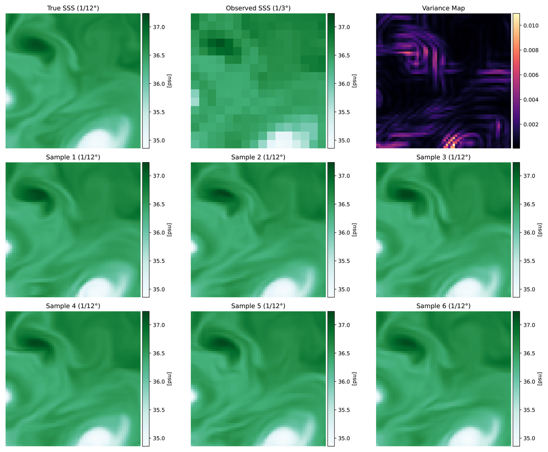
Figure 4 Collection of six $\mathrm{1}/\mathrm{12}\mathit{°}$ SSS patches generated for the same day of 2020 with six different inference noise initializations. The first row shows, from left to right, the reference high-resolution SSS patch, the $\mathrm{1}/\mathrm{3}\mathit{°}$ coarse SSS constraint, and the pixel-wise ensemble variance computed across the generated high-resolution SSS patches. The variance is larger in dynamically active regions where several fine-scale configurations remain compatible with the same coarse constraint as seen in the second and third rows. This spread is interpreted as a reconstruction-ambiguity diagnostic.

For DIFF-SST-SSH-BEST: from K=40 samples, we pick the realization that minimizes RMSE to the reference; this is not operational (it requires ground truth) but indicates the headroom available from the same trained prior.

For DIFF-SST-SSH-GE: we apply the gradient-enhancing guidance during inference and use the same central selection (closest-to-mean over K=15 guided samples), yielding higher-contrast outputs while remaining distribution-consistent.

In Table 2 we give for the six experiments the mean RMSE (psu) and SSIM during the test year 2020 over the test domain. These performances are computed from a daily basis. Conditioning on high-resolution auxiliaries at $\mathrm{1}/\mathrm{12}\mathit{°}$ improves SSS reconstructions from coarse SSS at $\mathrm{1}/\mathrm{3}\mathit{°}$. DIFF-SST outperforms DIFF-SSH and adding together SST and SSH improves the global RMSE. Indeed, as mentioned in Introduction, SST adds more information than SSH; SST provides the most precise guidance for the reconstruction of SSS. SST exhibits correlated structures at a very fine scale, unlike SSH, which is much smoother in the current GLORYS-based setup. A yearly average quantify these gains: DIFF-SST improves RMSE by ∼ 21 % relative to DIFF-SSH (0.045 vs. 0.057 psu); adding SSH on top of SST yields a further ∼ 11 % improvement (0.040 vs. 0.045 psu for DIFF-SST-SSH vs. DIFF-SST), indicating complementary mesoscale constraints from SSH.

To better understand the behavior of the six models, we present daily time series of RMSE over the year 2020. The y-axis is the mean RMSE computed over the Gulf Stream domain. As the order of magnitude is different for the six experiments, we compare DIFF-SST and DIFF-SSH in Fig. 5 and the 4 other models in Figs. 6. For the six experiments, across the seasonal cycle, errors peak in late spring–summer (day ∼ 170–200) and decrease towards winter. This timing coincides with seasonal maxima of eddy kinetic energy and frontal activity in the Gulf Stream region (Zhai et al., 2008; Joyce et al., 2019b, a).

As expected, in Fig. 5 DIFF-SST (magenta line) systematically outperforms DIFF-SSH (green line). In Fig. 6, DIFF-SST-SSH (magenta line) and RESAC (yellow line) display very similar daily RMSE time series, while DIFF-SST-SSH-BEST (blue line) provides a baseline/lower envelope because it uses the known reference for sample selection. DIFF-SST-SSH-GE (green line) has a larger RMSE than the standard DIFF-SST-SSH configuration. Thus, GE does not improve pixel-wise scores; rather, it is designed to test whether contrast-oriented inference can recover sharper structures at the cost of a moderate degradation in RMSE/SSIM. This distinction is important because RMSE and SSIM alone do not fully characterize frontal contrast and high-frequency variability.

For that purpose we compare different snapshots and then quantify the structural differences using gradient and spectral diagnostics. Visual differences in Fig. 7 are subtle at the scale of the full patch, and the figure should be interpreted as a qualitative illustration rather than as direct proof of sharpening. The effect of GE on small-scale structure is therefore assessed more directly in the next subsection using the gradient distribution and temporal Fourier spectrum. For all indices (RMSE, SSIM) computed yearly or daily the ranking of the models remains stable (Fig. 6). Thus, as using both auxiliary variables gives the best performances, DIFF-SST-SSH only will be used for the last comparisons.

5.2 Spatio-temporal structure and contrast enhancement

To assess fine-scale structure beyond pixelwise error, we analyse spatial gradient-magnitude distributions and temporal Fourier spectra over the 2020 test year. The reference gradient distribution (Fig. 8, left) is strongly peaked at low gradient values, corresponding to smooth regions, with a long tail representing fronts and energetic structures. The right panel shows the difference between model and reference gradient distributions for DIFF-SST-SSH, DIFF-SST-SSH-GE, and RESAC. All methods overestimate the proportion of weak gradients and underestimate intermediate-to-strong gradients, consistent with residual smoothing. DIFF-SST-SSH-GE reduces this bias over the low-to-intermediate range, indicating improved contrast and sharper reconstruction of fine-scale structure.

Temporal spectra provide a complementary view (Fig. 9). DIFF-SST-SSH and RESAC under-represent high-frequency (weekly-daily) variance, while DIFF-SST-SSH-GE remains closer to the reference across most frequencies and becomes slightly positive at the highest frequencies, consistent with recovered small-scale temporal energy. DIFF-SST-SSH-BEST does not uniformly improve all spectral ranges, illustrating that selecting a sample solely by minimizing RMSE does not guarantee optimal spatio-temporal consistency. Since BEST selection is not applicable operationally, it is interpreted only as a performance headroom indicator.

Overall, when pixelwise accuracy is the primary objective, DIFF-SST-SSH provides a strong operational choice with performance comparable to RESAC. When the fidelity of fronts and filaments is critical (e.g. frontal detection, feature tracking, or Lagrangian applications), DIFF-SST-SSH-GE offers a sharper representation of fine scales at a small cost in RMSE/SSIM. Across experiments, diffusion-based reconstructions are visually sharper than RESAC.

Table 1 Main characteristics of the six experiments.

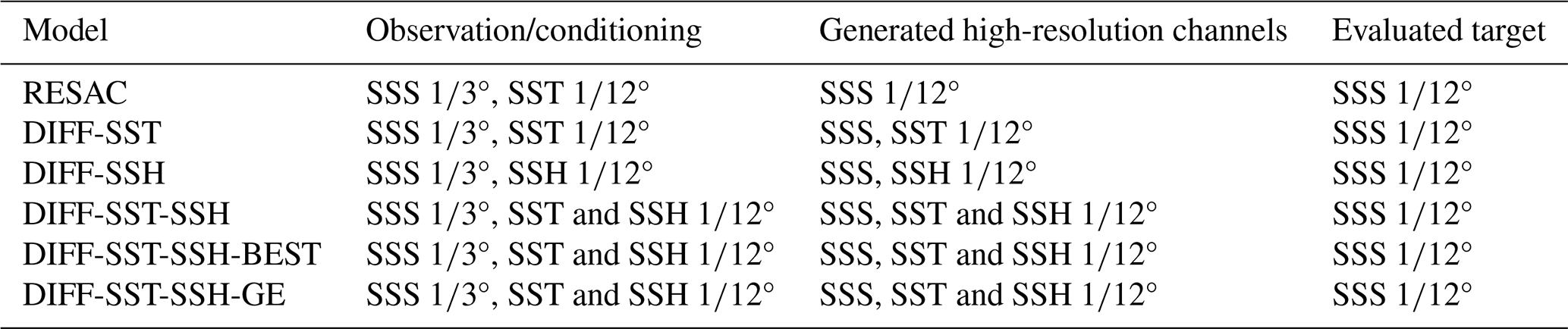
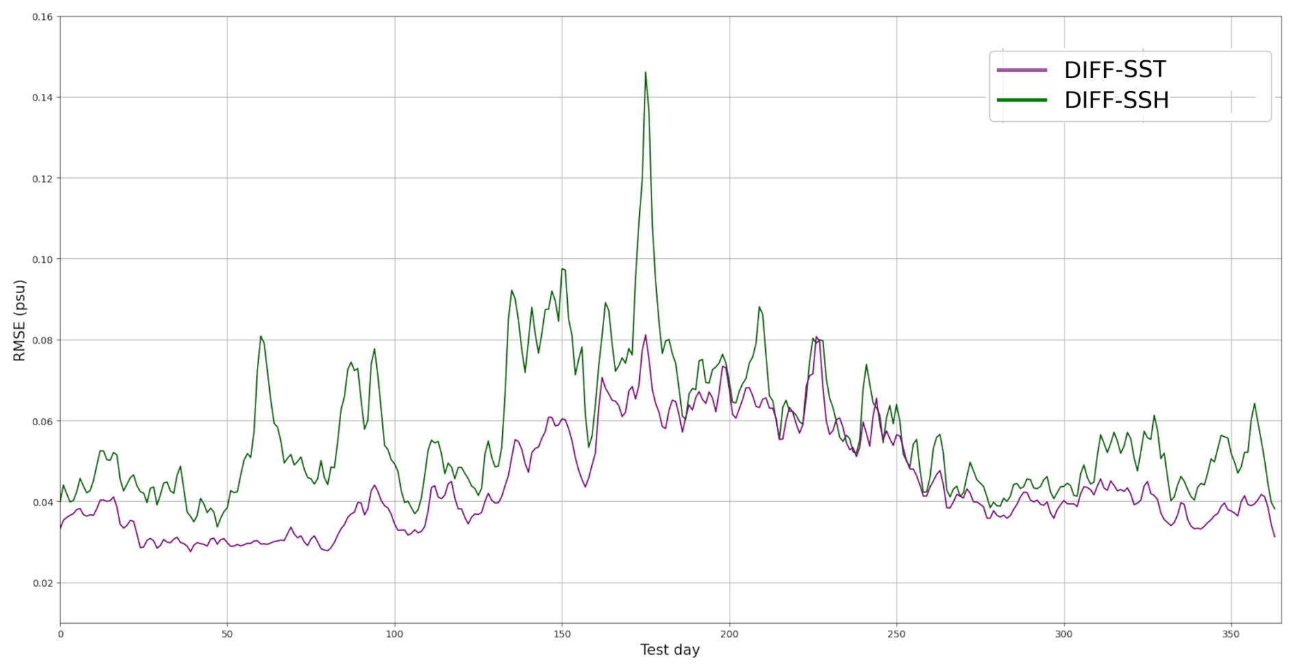
Figure 5 Daily RMSE of SSS $\mathrm{1}/\mathrm{12}\mathit{°}$ reconstructions over the year 2020 using DIFF-SST (purple) or DIFF-SSH (green). RMSE on the y-axis is the mean RMSE computed over the Gulf Stream domain. DIFF-SST provides systematically stronger guidance than SSH, with the largest gaps during the most energetic period (day ∼ 170–200).

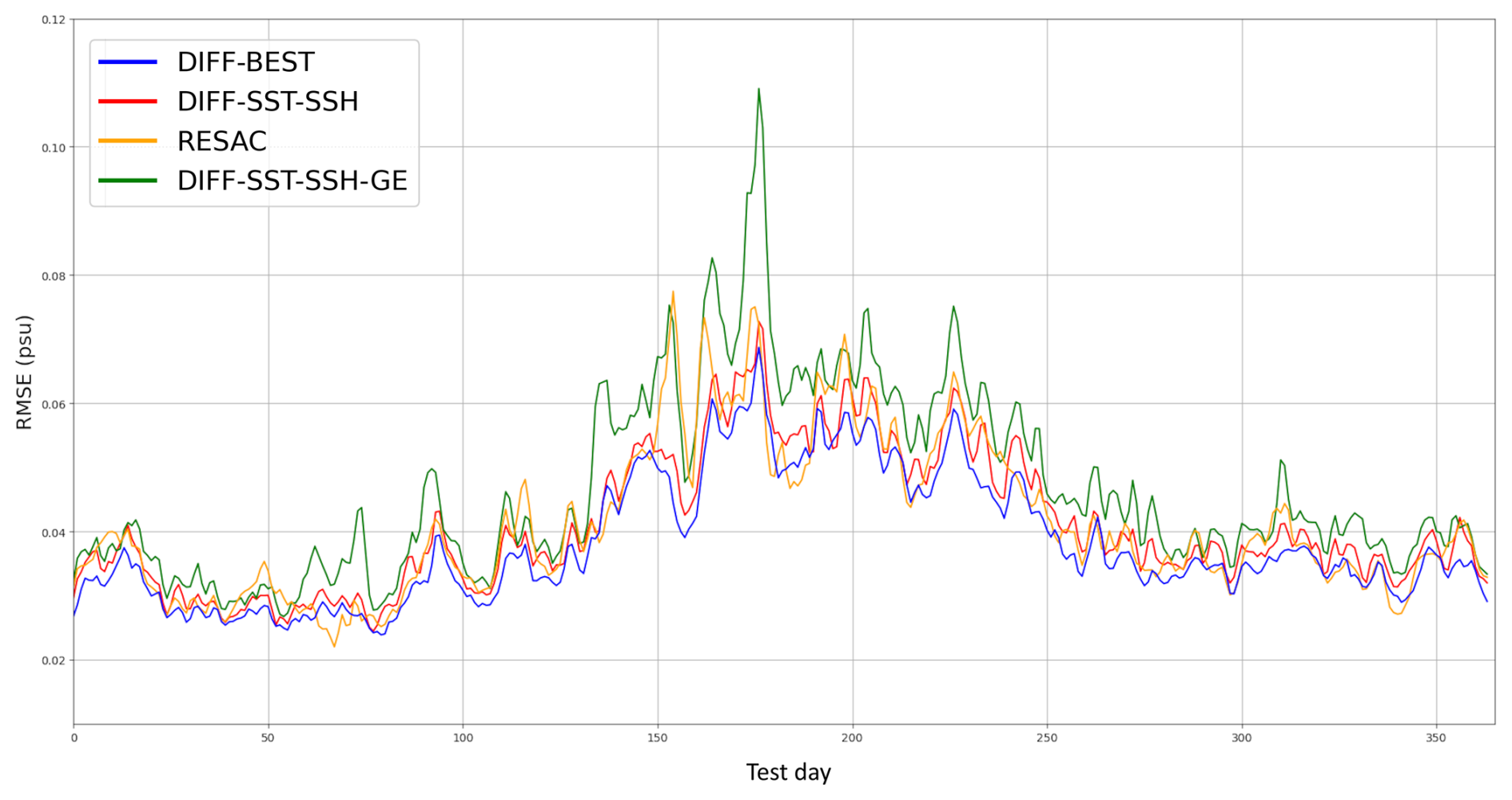
Figure 6 Daily mean RMSE of $\mathrm{1}/\mathrm{12}\mathit{°}$ SSS reconstructions over the year 2020 using DIFF-SST-SSH (red line), DIFF-SST-SSH-BEST (Blue), DIFF-SST-SSH-GE (green), RESAC (yellow). The x-axis represents the days of year 2020; RMSE, on the y-axis, is the mean RMSE computed over the Gulf Stream domain. DIFF-SST-SSH-BEST gives the lowest error envelope; the ranking of the models remains stable with respect to Table 2.

Table 2 Average metrics (RMSE and SSIM) for the year 2020 for the six experiments.

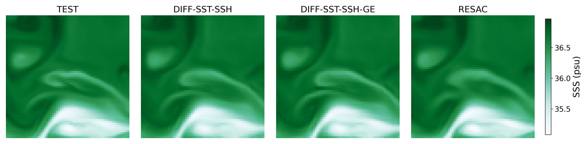
Figure 7 Example of SSS reconstruction at $\mathrm{1}/\mathrm{12}\mathit{°}$ for a Gulf Stream patch (day 120 of 2020). Left to right: REFERENCE (TEST), DIFF-SST-SSH, DIFF-SST-SSH-GE, and RESAC. All panels share identical color limits (psu).

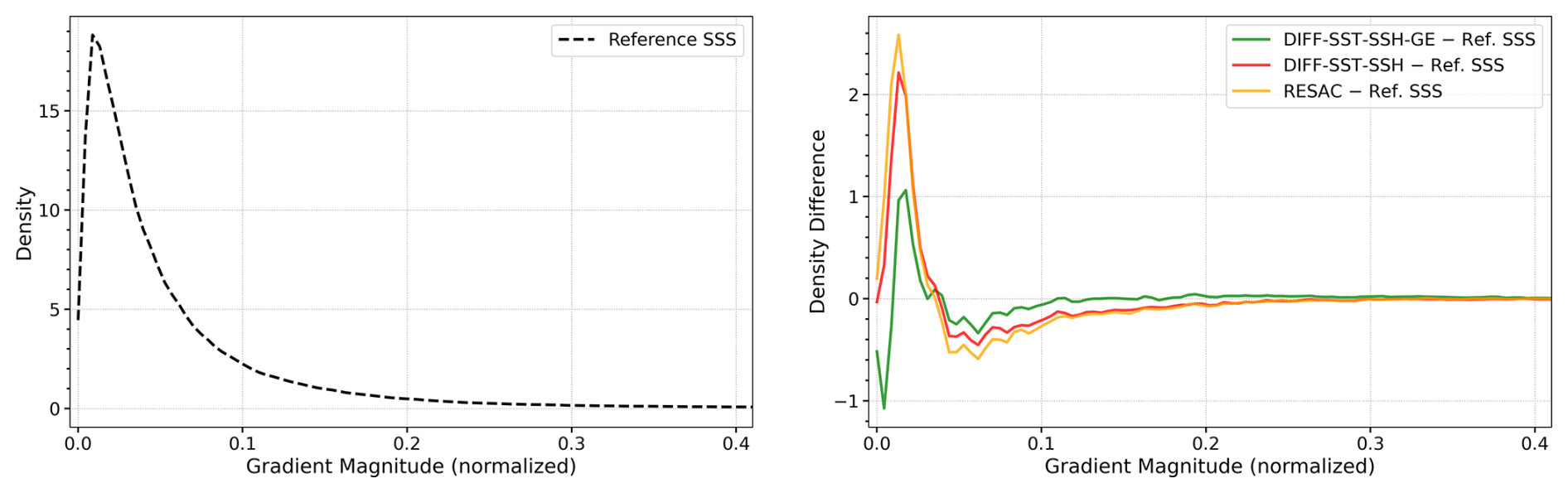
Figure 8 Left: gradient-magnitude distribution computed over all pixels and all images from the 2020 test dataset. Right: difference between each model distribution and the reference distribution for DIFF-SST-SSH (red), DIFF-SST-SSH-GE (green) and RESAC (orange). The high proportion of low gradients corresponds to smoother regions, while the tail corresponds to fronts and energetic structures. DIFF-SST-SSH-GE reduces part of the weak-gradient excess and recovers more intermediate-to-strong gradients, but the negative difference at the weakest gradients also indicates that the procedure may over-sharpen some regions.

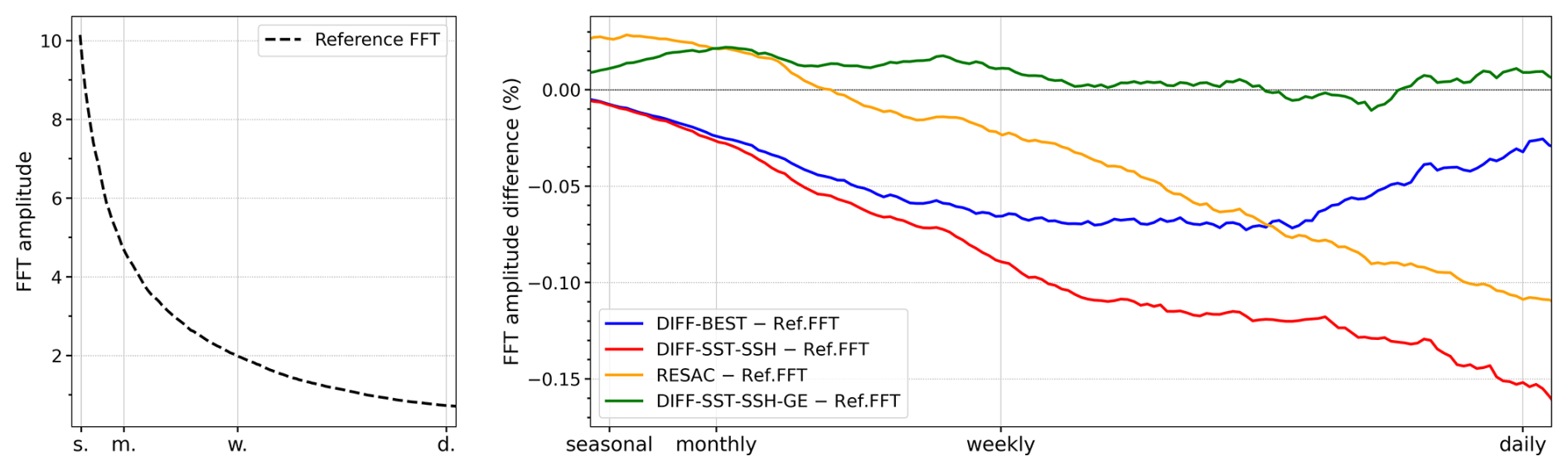
Figure 9 Left: reference mean temporal Fast Fourier Transform (RMT FFT) amplitude computed for each pixel over the 2020 test year and averaged over the study area. Right: percentage difference between each model mean temporal FFT amplitude and the reference. DIFF-SST-SSH-GE (green) increases high-frequency temporal energy relative to the standard diffusion configuration, but the positive difference over parts of the spectrum also indicates a possible over-amplification of small-scale variability.

6 Discussion

The experiments were designed to isolate methodological behavior in a controlled setting, using GLORYS as a dynamically constrained high-resolution reference and synthetically degraded SSS at coarse resolution. Within this framework, the results support four main conclusions and clarify several limitations that must be addressed before transfer to satellite SSS products.

6.1 Main findings and interpretation

High-resolution SST is the dominant auxiliary constraint for SSS downscaling in the Gulf Stream. Across the full 2020 test year, conditioning on SST yields substantially lower error than conditioning on SSH alone (Table 2; Fig. 5). This ranking is robust throughout the seasonal cycle, including the most energetic period (day ∼ 170–200) when reconstruction is most challenging (Figs. 5 and 6). This is consistent with the visual comparison of the three variables (Fig. 2): SST shares filamentary and frontal structures with SSS at finer scales, whereas SSH fields used here are smoother and mostly express mesoscale organization. In other words, SST appears to supply the local small-scale information that the model can “lock onto”, while SSH provides a weaker but complementary contextual constraint on the position and intensity of mesoscale features.

Adding SSH on top of SST provides a smaller but consistent gain. DIFF-SST-SSH improves on DIFF-SST in yearly-mean RMSE (Table 2) and remains competitive day-by-day (Fig. 6). The improvement is modest compared to the DIFF-SSH/DIFF-SST gain, but it is physically plausible. Yet this result should be interpreted with caution. It does not necessarily imply that SSH is intrinsically less relevant for constraining salinity fine scales; rather, it may reflect the comparatively smooth character of the SSH fields used in the present GLORYS-based setup. This point is particularly important in light of recent SWOT observations, which reveal a much richer fine-scale sea-surface height variability than previously accessible from conventional altimetry (Morrow et al., 2019; Archer et al., 2025). Recent studies also suggest that part of this small-scale and high-frequency SSH variability is still underestimated or only partially represented in present-generation 1/12° model-based products (Le Traon et al., 2019). Therefore, the weaker performance of SSH in our framework may be tied to the effective resolution and information content of the SSH product used here, rather than to the physical usefulness of SSH itself. Revisiting this question with SWOT-based or SWOT-constrained SSH products is a natural and important next step.

Diffusion with pseudo-inverse guidance is comparable to a strong CNN baseline under pixelwise metrics, while providing a conditional ensemble. With the closest-to-mean selection strategy (Sect. 5), DIFF-SST-SSH and RESAC yield very similar yearly-mean RMSE/SSIM (Table 2) and similar temporal evolution (Fig. 6). The diffusion approach should therefore not be interpreted as providing a large RMSE improvement over RESAC in this controlled experiment. RESAC remains a strong deterministic baseline, specifically designed for scale-adaptive downscaling. The added value of the diffusion framework is different: inference naturally produces an ensemble of plausible high-resolution fields conditioned on the same coarse observation (Fig. 4), and provides a diagnostic of reconstruction ambiguity.

Contrast-oriented guidance shifts the solution toward stronger small-scale contrast, but trades off against RMSE/SSIM and can over-amplify variability. The GE procedure increases gradient contrast relative to the standard DIFF-SST-SSH configuration (Figs. 8 and 9). At the same time, DIFF-SST-SSH-GE degrades RMSE/SSIM relative to DIFF-SST-SSH (Table 2), which is expected because RMSE favors smoother reconstructions and penalizes phase/position errors strongly. The gradient histogram also shows that GE reduces the proportion of weak gradients relative to the reference, and the temporal spectrum can exceed the reference over part of the frequency range. These diagnostics indicate that GE should be interpreted as a contrast-enhancing variant with a structural trade-off, not as a uniformly superior reconstruction. Model choice should therefore depend on the scientific objective: for applications prioritizing pixelwise accuracy, DIFF-SST-SSH is preferable; for applications where front and filament fidelity matters, GE-like guidance may be useful but should be tuned carefully.

6.2 What the diagnostics reveal beyond RMSE

The additional diagnostics clarify how errors differ between approaches. Gradient histograms show that all methods overpopulate weak gradients and under-represent part of the mid-high tail (Fig. 8), indicating residual over-smoothing relative to GLORYS. The GE variant partially corrects this by enhancing low/intermediate gradients, but the negative difference at the weakest gradients suggests that it may also over-sharpen the field by converting too many weak gradients into stronger ones. The temporal FFT analysis provides an independent view: DIFF-SST-SSH and RESAC under-represent high-frequency variance, while DIFF-SST-SSH-GE restores more energy but can exceed the reference over part of the spectrum (Fig. 9). Taken together, these results support a nuanced conclusion: the diffusion prior with standard selection is competitive under pixelwise scores, but its default samples remain slightly too smooth; targeted inference-time guidance can recover part of the missing variability, at the risk of over-amplification if the contrast guidance is too strong.

A related implication concerns sample selection. The “BEST” choosing strategy indicates headroom from the same trained prior (Table 2), but it is not operational and should not be over-interpreted as achievable performance. More importantly, the fact that “BEST” does not uniformly improve all diagnostics (e.g. FFT spectral behavior can differ) highlights that selecting samples solely to minimize RMSE does not guarantee spatio-temporal realism. This motivates future work on task-aware or physics-aware selection criteria that can be computed without access to truth.

6.3 Limitations and perspectives for transfer to satellite products

The present study was designed as a controlled methodological experiment, using GLORYS as a dynamically constrained high-resolution reference and synthetically degraded SSS as coarse observations. This framework is well suited to isolate the behavior of the diffusion-based downscaling method, but it also defines the main limitations of the present work and the conditions required for transfer to real satellite SSS products.

First, GLORYS is not assumed to be a perfect truth. It combines an ocean model with heterogeneous assimilated observations, and local inconsistencies between SSS, SST and SSH may remain. In this paper, GLORYS provides a complete multivariate gridded reference from which the diffusion model learns a GLORYS-consistent joint prior over SSS, SST and SSH. The generated reconstructions should therefore be interpreted as physically plausible within the GLORYS framework, not as guaranteed representations of the real ocean at all scales.

Second, the use of GLORYS avoids many of the complexities of L-band satellite retrievals, including sensor-specific biases, correlated retrieval errors, and irregular observation patterns (Boutin et al., 2014, 2021; Reul et al., 2020; Reverdin et al., 2024). While this is appropriate for method development, it means that the reported metrics should not be interpreted as direct estimates of performance expected for SMOS, SMAP, or multi-satellite products such as CCI products (Boutin et al., 2021). Real Level-4 SSS products are not clean low-pass versions of the true SSS field. For example, ESA CCI SSS is a multi-sensor Level-4 product derived from L-band radiometry; although it is sampled on a 0.25° grid, its effective spatial resolution is about 50 km and it provides uncertainty and quality information such as random error, unexplained variability, number of observations, outliers, and land/ice/SSS quality flags (Boutin et al., 2021). Such information should be used in future work to weight the observation guidance spatially and to mask unreliable pixels.

Third, the observation operator H used in this study mainly reflects spatial averaging and sub-sampling (Eq. 1). For real applications, H should mimic the targeted satellite product much more faithfully, including its effective footprint, grid, masks, and spatially heterogeneous uncertainty. Because pseudo-inverse guidance injects observational information at each denoising step (Song et al., 2023; Chung et al., 2024), the realism of H is a central requirement for domain transfer. In practical applications, the guidance term should therefore be uncertainty aware, matching H(X) to the satellite observation Y on the satellite grid while down-weighting uncertain, missing, or contaminated pixels.

Fourth, the auxiliary variables also have product-dependent limitations. High-resolution SST is an effective constraint in the present experiment, but observed infrared SST is unavailable under clouds. Daily gap-free Level-4 SST products may be distributed on fine grids, yet their local information content can degrade under persistent cloud cover because they rely on interpolation, microwave SST, previous clear-sky observations, in-situ data, and the analysis method (Embury et al., 2024; Donlon et al., 2012; Chin et al., 2017). In such regions, SST should be treated as an uncertain auxiliary constraint rather than as a uniformly reliable high-resolution observation. Similarly, the relatively weaker contribution of SSH in our experiments should not be regarded as definitive, as it may partly reflect the smooth character of the SSH fields in the present GLORYS-based setup. This balance may evolve as higher-resolution SSH observations become available, particularly through SWOT, which may provide a richer fine-scale dynamical constraint than that represented in current-generation reanalyses.

Fifth, the role of in-situ observations should be stated, such as Argo profiles within the proposed transfer framework. The high-resolution prior would still be learned from gridded reanalysis or simulation fields, while the observational constraint would be provided by a satellite SSS product through a product-aware observation operator. Argo, thermosalinograph data, moorings, drifters, and regional campaigns would then provide independent validation, calibration, and bias assessment.

Finally, operational deployment requires sample selection and uncertainty-calibration strategies that do not rely on access to the true high-resolution field. The closest-to-mean member used here provides one representative realization, while the ensemble spread shown in Fig. 4 provides a first diagnostic of reconstruction ambiguity. A calibrated uncertainty product would require testing the relationship between ensemble spread and actual reconstruction error using independent validation data. In that context, the diffusion framework is not only a source of multiple plausible reconstructions, but also a way to diagnose when the solution is weakly constrained, for example near coasts, under cloud-degraded auxiliary SST, or under strong satellite SSS retrieval uncertainty.

6.4 Concluding remarks

In a controlled Gulf Stream experiment, diffusion models guided by pseudo-inverse conditioning can downscale coarse SSS to $\mathrm{1}/\mathrm{12}\mathit{°}$ with accuracy comparable to a strong convolutional baseline, while naturally providing a conditional ensemble of plausible high-resolution fields. In the current GLORYS-based context, high-resolution SST is the primary source of fine-scale guidance; SSH adds complementary mesoscale context. A contrast-oriented guidance term can partially recover missing gradients and high-frequency temporal variance, at a small cost in RMSE/SSIM, highlighting an application-dependent trade-off between distortion metrics and structural realism (Wang et al., 2004; Ledig et al., 2017).

The next methodological frontier is transferability to satellite SSS. This requires (i) realistic product-aware observation operators and noise/mask models in H, (ii) uncertainty-aware weighting of satellite SSS and auxiliary SST/SSH constraints, (iii) strategies to mitigate reanalysis-to-satellite distribution shift, and (iv) operational sample selection and uncertainty calibration using independent in-situ validation. With these steps, diffusion-based downscaling has the potential to enrich present SMOS/SMAP/CCI products with GLORYS-consistent fine-scale structure, and to provide ensemble-based reconstructions that are directly usable for process studies and, ultimately, data-assimilation-oriented applications.

Appendix A: Denoising diffusion implicit models' architecture and gradient enhancement algorithm

We used a multi-channel U-Net that takes as input the stacked SSS, SST, and SSH fields and implements a standard Denoising diffusion implicit model (DDIM) procedure. Self-attention layers are included at the coarsest resolutions to capture long-range spatial dependencies, while convolutional residual blocks handle local interactions. This design provides a good balance between expressiveness and computational cost for high-resolution oceanographic images.

Algorithm A1 Gradient-Enhancing (GE) Algorithm.

Inputs: coarse SSS Y, observation operator H, pseudo-inverse H^†, contrast parameters γ,δ (with $\mathit{\gamma }-\mathit{\delta }>\mathrm{1}$),

ϵ-prediction diffusion model, time schedule $(v_i{)}_{i=\mathrm{0}}^N$ from 0 to T.

Initialize $X\sim \mathcal{N}(\mathrm{0},I)$

for i=T to 1 do

t←v_i,  $s\leftarrow v_{i-\mathrm{1}}$

${\mathit{\alpha }}_t\leftarrow {\displaystyle \frac{\mathrm{1}}{\mathrm{1}+{\mathit{\sigma }}_t^{\mathrm{2}}}}$,  ${\mathit{\alpha }}_s\leftarrow {\displaystyle \frac{\mathrm{1}}{\mathrm{1}+{\mathit{\sigma }}_s^{\mathrm{2}}}}$

$c_{\mathrm{1}}\leftarrow \mathit{\eta }\sqrt{\left(\mathrm{1}-{\displaystyle \frac{{\mathit{\alpha }}_t}{{\mathit{\alpha }}_s}}\right){\displaystyle \frac{\mathrm{1}-{\mathit{\alpha }}_s}{\mathrm{1}-{\mathit{\alpha }}_t}}}$

$c_{\mathrm{2}}\leftarrow \sqrt{\mathrm{1}-{\mathit{\alpha }}_s-c_{\mathrm{1}}^{\mathrm{2}}}$

${\mathit{ϵ}}_{\mathit{\theta }}\leftarrow \mathit{ϵ}\text{-prediction}(X,t)$

${\widehat{X}}_t\leftarrow {\displaystyle \frac{X-\sqrt{\mathrm{1}-{\mathit{\alpha }}_t}{\mathit{ϵ}}_{\mathit{\theta }}}{\sqrt{{\mathit{\alpha }}_t}}}$

if $t<N/\mathrm{4}$ then

$\mathit{\mu }\leftarrow {\mathrm{MeanPool}}_{\mathrm{2}\times \mathrm{2},\mathrm{2}}\left({\widehat{X}}_t\right)$

$g\leftarrow {\left({\left(H^{†}\left(Y\right)-H^{†}\left(H\right({\widehat{X}}_t\left)\right)\right)}^{\top }{\displaystyle \frac{\partial {\widehat{X}}_t}{\partial X}}\right)}^{\top }$

${\widehat{X}}_t\leftarrow {\widehat{X}}_t-\mathit{\mu }$

${\widehat{X}}_t\leftarrow \left(\mathit{\gamma }-\mathit{\delta }\sqrt{{\displaystyle \frac{\left|{\widehat{X}}_t\right|}{max\left|{\widehat{X}}_t\right|}}}\right){\widehat{X}}_t$

${\widehat{X}}_t\leftarrow {\widehat{X}}_t+\mathit{\mu }$

else

g←0

end if

$\mathit{ϵ}\sim \mathcal{N}(\mathrm{0},I)$

$X\leftarrow \sqrt{{\mathit{\alpha }}_s}{\widehat{X}}_t+c_{\mathrm{1}}\mathit{ϵ}+c_{\mathrm{2}}{\mathit{ϵ}}_{\mathit{\theta }}+\sqrt{{\mathit{\alpha }}_t}g$

end for

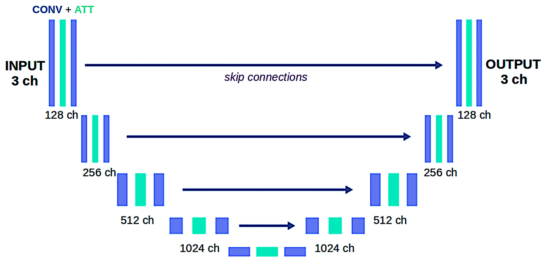
Figure A1 Architecture of the diffusion model, which uses a U-Net with skip connections, attention blocks (in green), and convolution blocks (in blue). The input and generated images are 64×64 in size and have up to three channels for SSS, SST, and SSH depending on the model configuration; the evaluated downscaling target is SSS.