Investigating the predictability of marine heatwaves at subseasonal to seasonal timescales in New Caledonia, South Pacific

Marine Heatwaves (MHWs) have emerged as one of the most important threat for marine ecosystems, with impacts such as coral bleaching, massive fish mortality and displacement of mobile fauna. In the context of climate change, it is urgent to develop strategies such as subseasonal to seasonal forecasting to help human societies adapt and react to the increasing frequency, duration and intensity of these events. Here we evaluate the predictability of MHWs at the scale of a South Pacific island country, New Caledonia, using ensemble forecasts from a dynamical coupled ocean-atmosphere model. We show that implementing a probabilistic approach where we extract information from the dispersion in the ensemble results in a higher skill than a deterministic approach where we simply compute the ensemble average. We find that longer, more intense, and wider MHWs, are more predictable than weaker, less intense, and shorter MHWs. We also find that the longest and widest MHWs occur in the cold season (June–October) during strong La Niña episodes, and that they can successfully be predicted up to 7 months in advance. In contrast, MHWs occurring during the warm season have poor or no predictability of more than a few weeks in advance. We discuss how this information can be efficiently transferred to marine stakeholders in terms of the usefulness and useability of the forecast. We recommend that future research should focus on identifying the drivers of different types of MHWs in order to understand their sources of predictability.

1 Introduction

Marine Heatwaves (MHWs), which are episodes of ocean temperature extreme ranging from a few days to a few months, represent one of the most dramatic manifestations of climate variability in the ocean (Oliver et al., 2021; Capotondi et al., 2024). MHWs can influence all the components of marine ecosystems (Smith et al., 2023; Smale et al., 2019; Wernberg et al., 2025; Starko et al., 2025), from benthic foundation species to plankton and megafauna, and drive a variety of responses such as coral bleaching, Harmful Algal Blooms, reduction of primary production (Noh et al., 2022) mass mortality of fish or kelp (Arafeh-Dalmau et al., 2020) and displacements of mobile species (Jacox et al., 2020; Welch et al., 2023). These effects can have severe consequences on the human societies who rely on the ocean for its material or immaterial value through aquaculture, fisheries, tourism, and cultural identity (Smith et al., 2021; Holbrook et al., 2022; Cheung et al., 2021; Fisher et al., 2021; Bambridge et al., 2021). While MHWs are a natural phenomenon, a significant increase in their frequency, duration and intensity has been detected in the historical record and attributed to anthropogenic climate change (Oliver et al., 2018; Capotondi et al., 2024). Climate projections show that the intensity and frequency of MHWs will continue to increase by the end of the century, with the magnitude depending on global greenhouse gas emissions (Frölicher and Laufkötter, 2018; Oliver et al., 2019). Importantly, the consequences of these long-term trends depend on the adaptive capabilities of the biological and societal systems, which are poorly known (Hobday et al., 2018; Witman et al., 2023).

In this context, subseasonal to seasonal forecasts are an important tool for stakeholders in order to monitor ocean conditions, react, and mitigate potential negative impacts of upcoming MHWs (Hobday et al., 2018; Holbrook et al., 2020; Sun et al., 2022; Hobday et al., 2024; Smith et al., 2025b). In the next few years, stakeholders will increasingly need to rely on such forecasts since their own previous experience will become less relevant as the climate system enters an unprecedented state (Spillman et al., 2021; Smith and Spillman, 2024; Hartog et al., 2023; Tommasi et al., 2017).

Early efforts at monitoring and forecasting ocean thermal stress focused on the risk of coral bleaching in summer (Spillman and Smith, 2021; Liu et al., 2018); however, as it has become apparent that coral reefs were not the only ecosystem to suffer from MHWs, a broader definition was proposed (Hobday et al., 2016, 2018) and is now widely adopted (Capotondi et al., 2024). With this approach, MHWs are defined as “prolonged periods of anomalous warm ocean temperature” relative to the normal seasonal cycle, and can therefore occur at any time, summer or winter.

Multiple studies have demonstrated the skill of various forecasting systems at seasonal timescales for MHWs and related metrics such as SST anomalies (Smith and Spillman, 2024), subsurface heat content anomalies (McAdam et al., 2023), occurence of MHWs (Jacox et al., 2022; Hu et al., 2025), number of MHW days (De Boisséson and Balmaseda, 2024), or the area affected by a MHW (Koul et al., 2023).

However, despite public availability of some operational products for the past few years (https://psl.noaa.gov/marine-heatwaves/, last access: June 2026; http://www.bom.gov.au/oceanography/oceantemp/sst-outlook-map.shtml, last access: June 2026), MHW forecasts are still not widely used (Smith et al., 2025b). Spillman et al. (2025) show that the adoption of forecasts into decision-making processes is challenging and suggest that improving the transfer of information from researchers to stakeholders requires ensuring that a MHW forecast is useful, useable and used.

Here we focus on the Coral Sea region, around New Caledonia, a tropical island in the South West Pacific Ocean highly vulnerable to MHWs because of its extensive coral reefs (Payri et al., 2019). We evaluate the MHW forecast skill of the french national weather center Météo-France System 8, comparing it to the european ECMWF SEAS5 forecasts. We focus on the first step of the framework of Spillman et al. (2025) and investigate whether our studied forecasts are useful (i.e., is the model configuration appropriate? Is the forecast skill sufficient?) and useable (are the forecast variables and timescales relevant to end users and easily interpretable?). Toward that end, we evaluate a wide range of MHW metrics describing various properties of MHWs (such as intensity, surface extent, duration, date of the next MHW and end date of the current MHW), using both a deterministic and a probabilistic approach. We also analyze the skill seasonality and its relationship with climate modes such as ENSO, taking advantage of the frequent initialization dates (first day of every month). Finally, we discuss the implications of our results in terms of usefulness and useability, thus laying the ground for the co-design of an operational product with local stakeholders.

2 Methods

2.1 Data

2.1.1 Forecast data

We use the Météo-France System 8 (Batté et al., 2021), launched in July 2021 and distributed by Copernicus Climate Change Service (C3S) (https://doi.org/10.24381/cds.68dd14c3). The modelling framework uses a fully coupled Earth System Model, which combines the NEMO ocean model (version 3.6), the ARPEGE atmosphere model, as well as land surface and sea ice models. The ocean model is run at 25 km resolution; however the outputs are degraded to 100 km for distribution by Copernicus. In addition to the continuously updated operational forecast, a hindcast was produced for the period 1993–2018; this retrospective dataset can then be used to evaluate the skill of the model by comparing the past forecasts with what actually happened. The hindcast and forecast periods are identical in all respects, except for the number of members. Each run lasts 7 months (212 d) and includes 25 members for the hindcast period (1993–2018) and 51 members for the forecast period (July 2021–present). The members differ by small perturbations in their initial conditions. Hence dispersion within the ensemble represents observational uncertainties and capture a range of plausible scenarios. The model forecasts are initialized at the beginning of each month, using reanalysis data (ERA5 for the atmosphere and GLORYS12V1 for the ocean).

The daily modeled SST data were downloaded from Copernicus Climate Data Store using the “cdsapi” python package. The data structure includes 5 dimensions: the initialization date (the first day of each month for the 26 years of hindcast and 3 years of forecast), the lead time (the time elapsed since the initialization, between 0 and 212 d), the number of members (25 for the hindcast period or 51 for the operational period) and the longitude and latitude.

In addition, we perform the same analyses with the European Centre for Medium-Range Weather Forecasts (ECMWF) Seasonal Forecast System SEAS5 (Johnson et al., 2019), also distributed by Copernicus C3S. This system is similar to Météo-France System 8: the main differences being the use of the IFS (Integrated Forecast System) atmosphere model instead of ARPEGE, the hindcast and forecast periods (1981–2016 and 2017–present) and the initialization scheme, but the ocean model and the number of members are identical.

2.1.2 Verification data

We use the GLORYS12V1 ocean reanalysis as our reference verification ocean dataset, hereafter referred to “observations”. GLORYS assimilates in-situ and satellite data, and has been shown to be a realistic reconstruction of ocean conditions (Lellouche et al., 2021). Importantly, GLORYS uses the same ocean model as the Météo-France System 8 (NEMO version 3.1) and is used during the initialization of the forecasts. Therefore, using GLORYS as our reference offers more consistency than using SST satellite data or other reanalysis ocean products, which allows us to isolate the forecasting errors from other sources of uncertainties (such as errors in the initial conditions). The data was downloaded from Copernicus Marine Data Store (https://data.marine.copernicus.eu/product/GLOBAL_MULTIYEAR_PHY_001_030, last access: June 2025) using the Copernicus Marine Toolbox API (“copernicusmarine” python package). For the ECMWF forecasts, the verification was performed with the ORAS5 reanalysis (https://data.marine.copernicus.eu/product/GLOBAL_MULTIYEAR_PHY_ENS_001_031, last access: November 2024).

2.2 MHW definition and metrics

We use the Hobday et al. (2016) MHW definition, which describes a MHW as a “prolonged period of anomalously warm water”. Contrary to heat stress indices tailored for coral bleaching risk in summer – such as Degree Heating Weeks (Liu et al., 2018)) – this definition is general and includes winter MHWs. We chose the hindcast period (1993–2018) as the baseline and kept a fixed baseline rather than removing the decadal warming trend. While using a detrended baseline (i.e., a baseline computed from a timeseries where the long-term lienar trend has been removed) is appropriate for certain applications where discriminating between short term variability and climate change is necessary, here we wish to include any warm episode that could impact socio-ecosystems. It should also be noted that keeping the warming trend may artificially inflate the skill reported here, which may not accurately reflect the ability of the model to capture seasonal variability (Smith et al., 2025a). The 90th percentile is computed using a temporal window of 11 d.

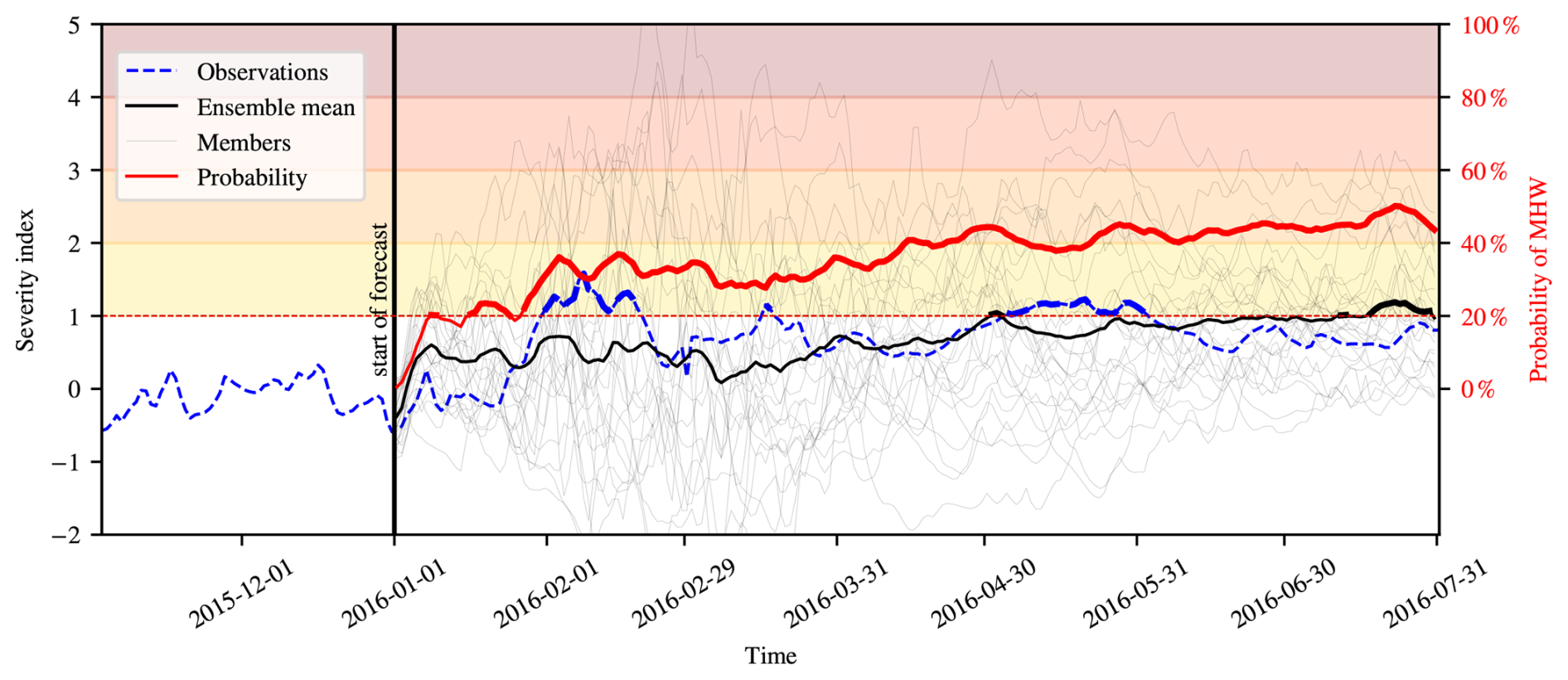
Figure 1 Example of forecast started on 1 January 2016 and averaged over the New Caledonia EEZ. The blue line is the observed severity index. The grey lines are the severity index for each member, with the ensemble mean shown in black. Note that the lines are thicker when they exceed a value of 1, indicating a MHW state. The red line is the forecasted probability of a MHW, computed as the proportion of members in a MHW state (of any category); it is thicker when it exceeds a certain probability threshold (here chosen at 20 %). A thick black line means that the deterministic forecast predicts a MHW, and a thick red line means that the probabilistic forecast predicts a MHW. The severity and the probability were computed for each grid point and then averaged for the NC EEZ.

Based on this definition, we create a daily gridded field with two variables:

• The severity index (Sen Gupta et al., 2020) is a daily index of temperature anomalies, scaled to the local variability $\left(\mathrm{severity}\mathrm{\_}\mathrm{index}=\frac{\mathrm{SST}-\mathrm{SST}{}^{\mathrm{clim}}}{\mathrm{SST}{}^{\mathrm{PC}\mathrm{90}}-\mathrm{SST}{}^{\mathrm{clim}}}\right)$: a value of 0 represents the climatological average (SST^clim), a value of 1 represents the 90th percentile (SST^PC90), a value of 2 represent a SST anomaly twice as large as the 90th percentile, etc. Note that this metrics is continuous and can reach negative values. Contrary to using categories based on fixed percentile (e.g. 90, 95, 98, etc.), this approach is unbounded and categories, as defined below, can be added as temperatures warm even with a fixed baseline. A MHW event is defined by the severity index exceeding 1 for at least 5 d; in addition MHWs separated by less than 2 d are merged into a single event.

• The MHW category (Hobday et al., 2018) represents the severity at the peak of the MHW event (category 1 corresponds to a peak severity between 1 and 2, category 2 between 2 and 3, etc.). It should be noted that the category is defined a posteriori for the entire MHW and remains constant for its entire duration. Thus, it gives no information about the evolution of the MHW over time.

The computation of the baseline and MHW category was performed using the “marineHeatWaves” python package written by Eric C. J. Oliver: https://github.com/ecjoliver/marineHeatWaves (last access: October 2023) and all further computations were done using the “xarray” python package (Hoyer and Hamman, 2017).

The severity index and the category indicate the intensity of thermal stress at different temporal scales, which may have consequences for predictability. The severity reflects the SST anomaly at a daily scale while the category reflects the peak SST anomaly at the scale of the MHW. On the one hand, the severity index, being a continuous variable, gives more precise information and should thus be more difficult to predict accurately. On the other hand, the use of thresholds for the category can amplify small differences and result in inflated errors (for instance, a severity of respectively 1.99 and 2.01, despite being very close, corresponds to different categories). In addition, the computation of forecasted MHWs does not include information prior to the start date, which means that if a forecast starts during a MHWs but after its peak, the forecasted category will only correspond to the decline phase and will be lower than if the entire MHW is included.

The MHW category and severity are then used to derive additional metrics that synthesize information at different spatio-temporal scales.

• the number of MHW days per month (category 1 or higher) is computed from the daily category.

• the surface fraction of a certain region covered by a MHW (category 1 or higher) is computed from the daily category.

• the monthly maximum of severity is computed from the daily severity index.

These metrics are potentially easier to predict than the category or severity at each day and each location, since they provide integrated information on the exposure to MHWs during a certain period or region. The quantification of their predictability is our focus, and the eventual choice of metrics by stakeholders will represent a trade-off between spatio-temporal resolution and forecast accuracy.

The metrics are computed for all members of the forecast and the reanalysis (light grey lines and dashed blue line on Fig. 1). The ensemble mean (black line on Fig. 1) is then computed as the average of the metric value of each member (for instance, the member average of the severity).

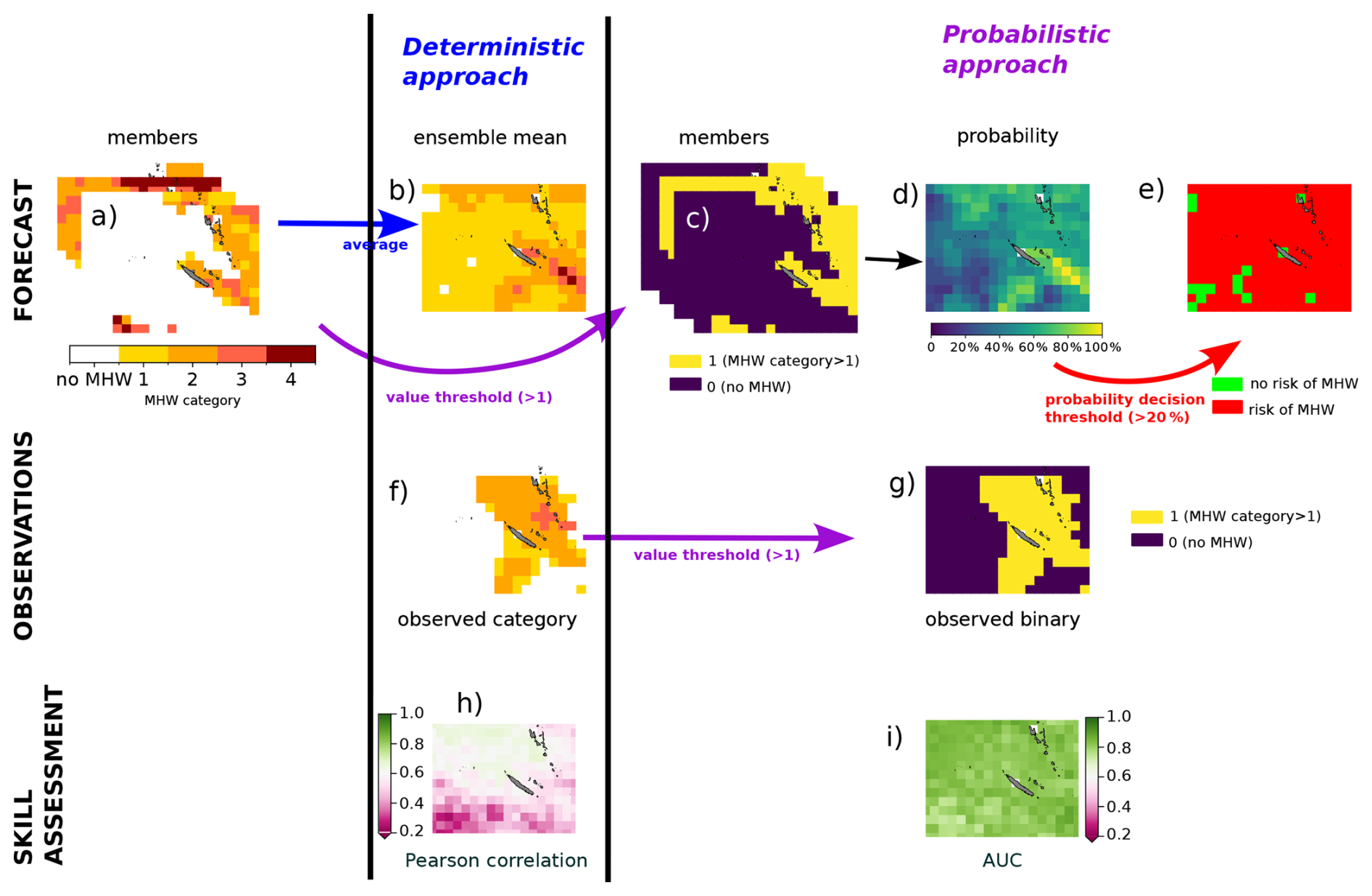
Figure 2 Schematic showing the two approaches (deterministic and probabilistic) used to evaluate forecast skill. The first row shows the forecast data; the second row shows the validation data (the observations); the third row shows the skill, computed from the two panels above. In the deterministic approach, all the MHW metrics calculated from the members (a) are averaged (b), and then the correlation between the ensemble mean and the observations (f) is computed; this correlation (h) represents the deterministic skill. In the probabilistic approach, a value threshold is chosen to define the event/nonevent (c) (here the “event” is a MHW, i.e category≥1) and the probability of this event is computed as the proportion of members that predict the event (d). The probability is then compared to the actual occurence in the observations (g) to construct the ROC curve and compute the AUC (i). Finally, a decision threshold can be chosen to turn this probability into a binary forecast (e) (in this case there is a MHW if more than 20 % of members predict a MHW). The process is repeated for other MHW metrics and value thresholds defining other pairs of event/nonevent. The verification is performed for each grid point, in order to obtain skill maps (Figs. A4–A6). ROC: Receiving Operating Characteristic. AUC: Area Under the Curve.

2.3 Verification

The verification of a forecast consists in the quantification of the differences between the forecast and an observational reference (in our case the GLORYS reanalysis) by various metrics for skills. In addition, the added-value of the forecast is evaluated by comparing it to a simplified reference forecast: here we use a persistence forecast, which is the initial value kept constant for the 7 months. Since the MHW metrics are defined as anomalies, the persistence is in our case equivalent to more complex references such as the climatological seasonal cycle or the persistence of anomalies. Thus outperforming the persistence is not trivial and requires a high level of skill. We performed the verification with the “climpred” python package (Brady and Spring, 2021).

We use both a deterministic and a probabilistic approach, summarized in Fig. 2.

2.3.1 Deterministic forecast skill

The deterministic forecast skill is computed based on the forecast ensemble mean, i.e. the average value of all the members, for each metric considered. Four deterministic metrics are defined: the severity index (daily), the number of MHW days per month (monthly), the monthly maximum severity and the surface fraction in MHW state (daily). The skill is quantified using the Pearson correlation coefficient between observation and forecast ensemble mean for each grid point and for each lead time (ie, between 384 pairs of points for the 32 years × 12 start months). While this score does not give an estimate of the absolute error of the forecast, it allows for easy comparison between variables of different magnitudes, which is our primary objective. A Pearson coefficient higher than 0.7 is generally considered indicative of a strong correlation while a value lower than 0.5 suggests a weak correlation (Schober and Schwarte, 2018).

2.3.2 Probabilistic forecast skill

With a probabilistic approach, the probability of event occurrence is first computed as the proportion of members forecasting this event. A probability decision threshold can then be chosen to determine whether the ensemble as a whole predicts the event or not (Fig. 2, red arrow). Once the forecast has been classified as an “event” or “non-event”, it can be compared to observations to determine if the prediction was a hit (both the forecast and the observations are “event”), a false alarm (forecast is “event” but observation is “non-event”), a miss (forecast is “non-event” but observation is “event”) or a true negative (both “non-event”). This process is then repeated for a large number of forecasts (here the 32 years × the 12 start dates = 384) to produce the contingency table, which consists of four values: the numbers of hits, misses, false alarms and true negatives among the 384 values. Various metrics can be computed based on this table, such as the hit rate $\left(\frac{\mathrm{hits}}{\mathrm{hits}+\mathrm{misses}}\right)$ and the false alarm rate $\left(\frac{\mathrm{false}\mathrm{alarms}}{\mathrm{hits}+\mathrm{false}\mathrm{alarms}}\right)$. At each location, the ROC curve (Receiving Operating Characteristic) is constructed by repeatedly selecting a decision threshold (10 %, 20 %, 30 %, etc.) and computing the corresponding hit rate and false alarm rate. Thus, the ROC is a graphic with the hit rate as a function of the false alarm rate. A “perfect” ROC reaches the upper left corner, which indicates that all events where detected (hit rate = 1) and no events were falsely predicted (false alarm rate =0). The diagonal represents the absence of skill: the hits and false alarms increase in equal proportions. The Area Under the Curve (AUC) is computed as the integral of the ROC curve: it varies between 0.5 (ROC curve is the diagonal) and 1 (the curve reaches the top left corner). Since the AUC is constructed using a range of decision thresholds, it is not sensitive to the choice of a particular threshold; rather it allows an operator to choose a threshold, which compromises between the number of true positive and false alarms depending on what the operator decides to be most important for his decision making (see the Discussion section). The AUC is a commonly used measure of skill, with a score of 0.8 generally considered to represent a useful forecast (Çorbacıoğlu and Aksel, 2023). The AUC measures the discrimination, i.e. the ability of the forecast to distinguish between events and nonevents (Ben Bouallègue and Richardson, 2022). In addition, the calibration of the forecast was evaluated using reliability diagrams.

We selected four variables and defined two binary conditions for each, representing the level of exposure to MHWs:

• The MHW category was used to define the intensity of the exposure: moderate ($\mathrm{1}\le \mathrm{category}<\mathrm{2}$) and severe (category≥2).

• The severity index was also used to define the intensity of the exposure: moderate ($\mathrm{1}\le \mathrm{severity}\mathrm{\_}\mathrm{index}<\mathrm{1.5}$) and severe (severity_index≥1.5). The choice of 1.5 as the threshold for severity, rather than 2 like the category, was to ensure that the computation of scores is meaningful (see Appendix for details).

• The number of MHW days per month was used to define the duration of the exposure: short ($\mathrm{5}\le \mathrm{numdays}<\mathrm{15}$) and long (numdays≥15).

• The surface fraction was used to define the spatial extent of the exposure: narrow (10 % $\le \mathrm{surf}\mathrm{\_}\mathrm{frac}<\mathrm{50}\mathit{\%}$) and wide (surf_frac≥50 %).

Finally, we defined two additional metrics to predict a change of state from normal conditions to MHW (i.e. category≥1) or from MHW to normal conditions. For this we computed the number of days between the beginning of the forecast and the next change of state. These metrics may have direct relevance to policymakers who can evaluate how much time is available to prepare for a coming MHW or to plan for the continued monitoring of an ongoing MHW until its termination. These metrics differ from the ones previously described since they are not defined for each time step (daily or monthly) but have only one value for each forecast. Since these metrics do not depend on lead time and only have one value per forecast, we cannot evaluate the skill using the same verification analysis as the other metrics. Instead, we simply computed the correlation between the forecasted and observed values. The occurence of a MHW was defined in a probabilistic manner: the forecast was classified as “in MHW state” if more than 20 % of the members were in a MHW state (the choice of this probability threshold was based on the ROC analysis, see Discussion section).

3 Results

We evaluate the forecast skill of MHWs using different approaches, in order to find the “best” forecast for stakeholders. We first compare the skill of different MHW properties (such as duration and intensity) using a deterministic approach. We then adopt a probabilistic approach in order to compare different types of MHWs (such as short and long MHWs). We finally investigate the influence of the spatial scale on the forecast skill (maps versus regional averages), as well as the large scale context (season and ENSO phase).

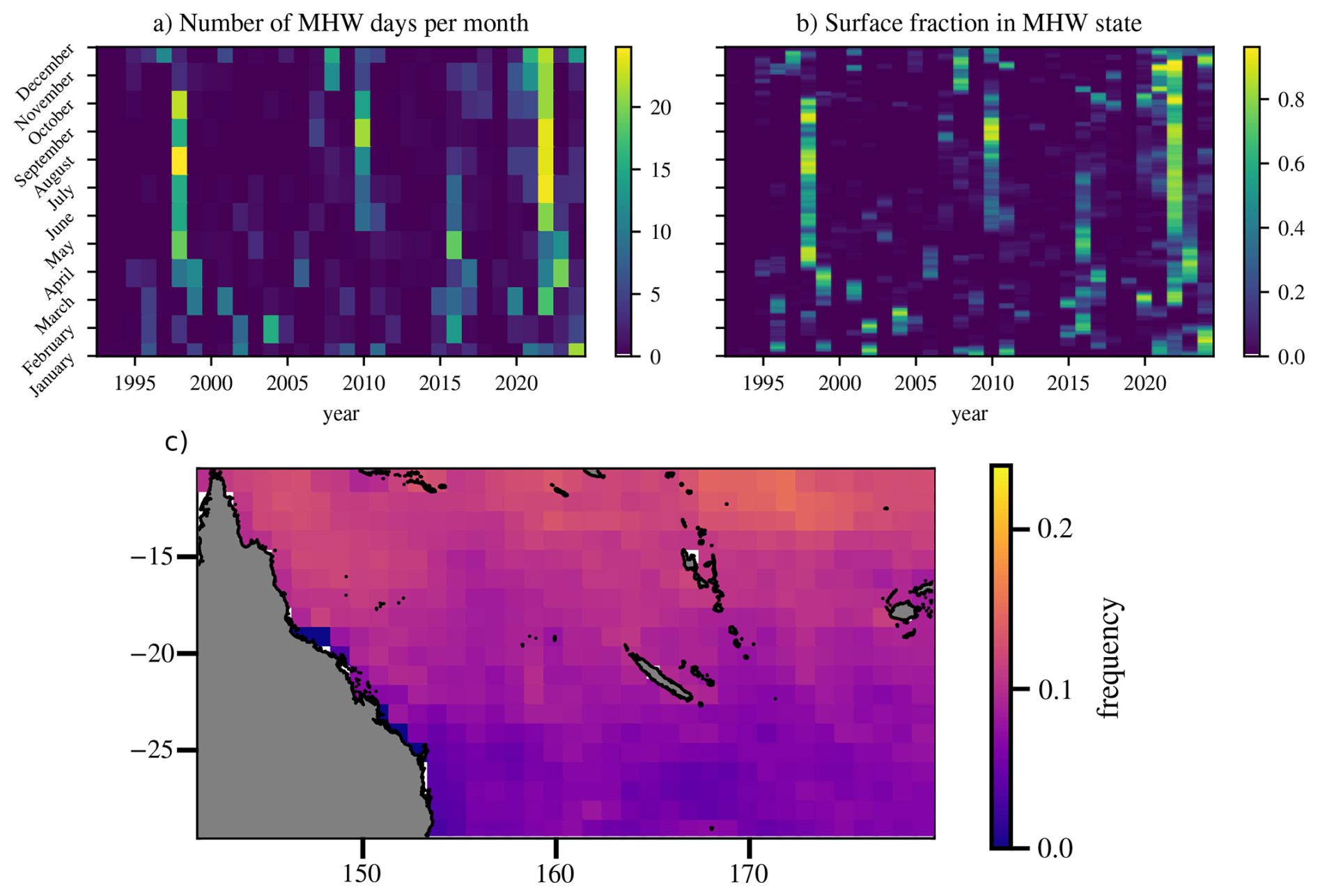
Figure 3 Exposure of New Caledonia to MHWs between 1993 and 2024 in the observations (here the Glorys reanalysis): number of MHW days per month averaged in the NC EEZ (a), surface fraction of the EEZ in MHW state (b) and the climatological frequency of MHWs (i.e., the number of MHW days divided by the total number of days) (c).

3.1 Exposure of New Caledonia to MHWs

Overall, the waters around New Caledonia experience MHWs about 10 % of the time (Fig. 3c). This is consistent with the statistical definition of MHWs as days where the SST is above the 90th percentile, or in other words the 10 % warmest days. A spatial gradient emerges, with MHWs more frequent at low latitudes (15 %) than high latitudes (5 %). This may be caused by the minimum 5 d duration criteria of MHWs that is less frequently met at higher latitudes due to higher variability as also reported in Lal et al. (2026) or because of spatial differences in the recent warming trend (i.e., SST has increased faster in that region between 2018–2024, since the end of the baseline period).

The exposure to MHWs of the New Caledonia EEZ exhibits seasonal differences (Fig. 3a, b). The cold season (April–September) experiences two regimes: prolonged and wide MHWs for a minority of years (1998, 2010 and 2022) and almost no MHWs for the rest of the years. Interestingly, these 3 “unusual” years coincide with particularly strong La Niña events (Pagli et al., 2025), although some other strong La Niña years show no particularly intense MHWs (such as 2000, 2008, 2011 or 2021). On the contrary, the warm season (October–March) generally experiences shorter MHWs every year that can episodically cover a large portion of the area.

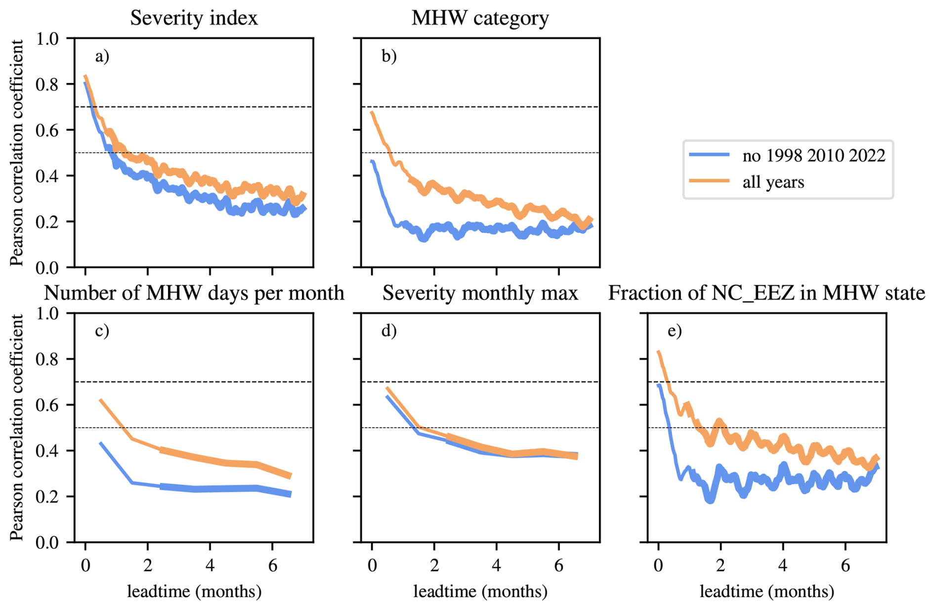
Figure 4 Deterministic forecast skill of the Météo-France System 8 for 5 MHW metrics (described in the section “MHW definition and metrics”), quantified by the Pearson correlation coefficient. For orange lines all years were included in the computation, but for blue lines the Niña years 1998, 2010 and 2022 were removed. The lines are thicker when the forecast skill is better than persistence. A Pearson coefficient higher than 0.7 indicates a strong correlation (dashed horizontal line). Verification scores were computed for each grid cell and then averaged over the NC EEZ for all metrics except the surface fraction. Note: correlation is significant everywhere (p-value < 0.05, not shown).

Figure 5 Deterministic forecast skill of the ECMWF system SEAS5 (cf legend of Fig. 4).

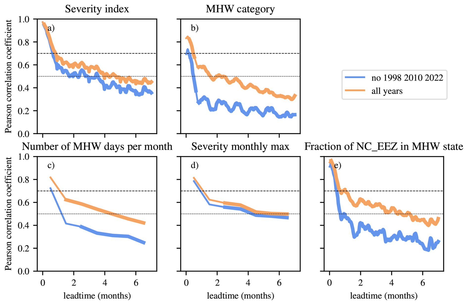
3.2 Deterministic scores

We computed the forecast skill of two forecast systems (Météo-France and ECMWF) for 5 deterministic metrics, first by including the entire hindcast period (orange lines in Figs. 4 and 5) and then by excluding the 3 “unusual” years identified above (1998–2010–2022, blue lines in Figs. 4 and 5). This allows us to evaluate how much of the skill is contained in these 3 years, and the quality of the forecast that can be expected in a “normal” year. We also investigate whether skill can be improved by looking at metrics aggregated over a certain region (such as the EEZ of New Caledonia) and thus ignoring spatial variability within this region. We computed MHW metrics based on the spatial average of the SST in this region, but this approach only resulted in a very slight improvement in skill compared to the computation of the skill metric in each grid point (Fig. A7). Thus we present here the skill computed in each grid cell and then spatially averaged in the region of interest. Skill maps show that there is very little spatial variation within the domain (Fig. A4).

Several conclusions can be drawn from this analysis:

• The skill of the Météo-France system is poor, rarely exceeding a Pearson coefficient of 0.7 even at short leadtimes and falling below 0.5 after the first month (Fig. 4d). However, at longer leadtimes it is generally able to beat the persistence forecast; but given the weak correlation at these lead times, these forecasts have an overall limited usefulness. The ECMWF system performs better, with very strong correlations during the first month and a higher skill than persistence (Fig. 5), but the skill is also very low at longer lead times.

• Some metrics have a higher skill than others. The severity monthly maximum has the highest skill, especially at longer leadtimes, while the skill for the category is consistently the lowest. Unexpectedly, there is no significant improvement for metrics at larger spatio-temporal scales: the skill of the daily severity (Fig. 4a) is comparable to the skill of the number of MHW days per month (Fig. 4c) and the surface fraction in MHW state (Fig. 4e). The difference in skill between severity (Fig. 4a) and category (Fig. 4b) is particularly interesting, as it suggests that the arbitrary thresholds (i.e., a severity higher than 1 for at least 5 d) might be blamed for the poor performance of category forecasts.

• The skill systematically decreases when the 3 La Niña years with long MHWs are removed (Fig. 4, blue lines). This clearly highlights the importance of considering the drivers of MHWs to understand their predictability: here most of the skill is linked to three La Niña events. The decrease of skill without these 3 years occurs for all metrics but is less important for the severity index (Fig. 4a) and the severity monthly maximum (Fig. 4d).

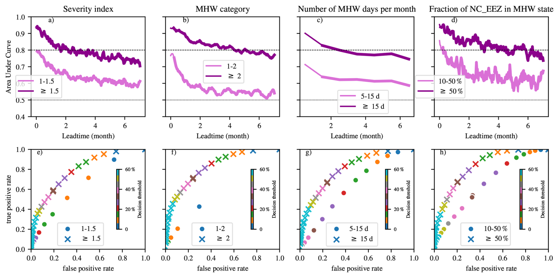
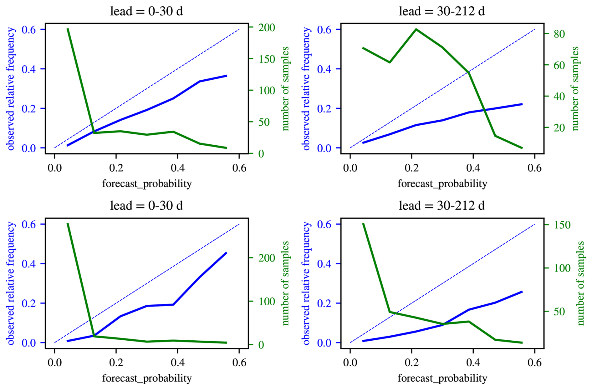
Figure 6 (a)–(d) Probabilistic forecast skill of the Météo-France System 8, measured with the AUC, for 4 MHW metrics (1 in each column). Each metrics has two levels of exposure: high (dark purple lines) and moderate (light purple lines). Values of 1 indicate perfect skill and values of 0.5 indicate no skill; values higher than 0.8 indicate good skill (horizontal dashed lines). (e)–(h) the corresponding ROC curves, averaged over all lead times. The black star shows a possible choice of optimal threshold (closest position to the top left corner, i.e. minimizing false alarms while maximizing hits), which may be different for the intense exposure (crosses) and the moderate exposure (circles).

Figure 7 Probabilistic forecast skill of the ECMWF system SEAS5 (cf legend of Fig. 6).

3.3 Probabilistic scores

Here we evaluate the ability of the two forecast systems to predict the probability of different levels of exposure (dark and light purple lines), defined in terms of intensity (first two columns in Figs. 6 and 7), duration (third column in Figs. 6 and 7) and spatial extent (fourth column in Figs. 6 and 7).

Both forecast systems perform well with the probabilistic approach, although the skill of ECMWF (Fig. 7) is again higher than Météo-France (Fig. 6). Reliability diagrams show that the forecasts are well-calibrated, although both systems tend to overpredict MHWs (Figs. A10–A13). For the most intense events in particular (dark purple lines in Figs. 6 and 7), the Area Under the Curve (AUC) remains above 0.8 for at least 4 months in the Météo-France forecasts and 6 months in the ECMWF forecasts. In addition, probabilistic forecasts tend to be better than persistence, even at very short leadtimes, while the deterministic forecasts only start to outperform the persistence after the first few weeks or even months (bold lines in Figs. 4–7). While probabilistic and deterministic skill are impossible to compare directly since they are quantified with different scores (the Area Under the Curve and the Pearson correlation coefficient, respectively), these results suggest that the probabilistic approach improves the quality of the forecast. Indeed, forecasts are generally considered to have no skill when the Pearson coefficient and the AUC are below 0.5, and to have “good” skill when the Pearson coefficient is above 0.7 or the AUC is above 0.8 (Horizontal dashed lines in Figs. 4 and 7). Even if these reference values for what constitutes “good skill” are subjective and could be debated, there is a clear contrast between the deterministic and probabilistic scores: deterministic scores fall under these thresholds much quicker than probabilistic scores. For instance, all AUC values are above 0.5 for the entire forecast (7 months), while only some metrics have a Pearson coefficient above 0.5. Pearson coefficients only exceed 0.7 at very short leadtimes, while AUC commonly exceeds 0.8 for many months. As an illustration, Fig. 1 shows how a MHW in February 2016 can be detected 1 month in advance by a probabilistic forecast (red line) but completely missed by a deterministic forecast (black line).

The bottom panels of Figs. 6 and 7 show the ROC curves that the AUC scores (top panels) are computed from and guide the interpretation of AUC values. For instance, for the severity index, the most extreme exposure (severity≥1.5) has a AUC that varies from 0.95 to 0.75, averaging 0.8 (Fig. 6a, dark purple line). The corresponding ROC curve (Fig. 6e, crosses) is well above the diagonal, and is closest to the top left corner with a decision threshold of 20 % (red cross). With this optimal threshold, the forecast will achieve an 80 % hit rate and a 40 % false alarm rate. Depending on the user, this might be considered useful or not (see the Discussion section).

The shift between the dark and light purple lines (Figs. 6 and 7) show that the level of exposure significantly influences the skill. Thus exposure to MHWs of high intensity (defined with the severity index above 1.5 or the category at MHW scale above 2) is more predictable than MHWs of moderate intensity; exposure to longer MHWs (more than 15 d per month) is more predictable than shorter; exposure to wider MHWs (covering more than 50 % of the EEZ) is more predictable than narrower MHWs. On the other hand, the skill is weakly influenced by the initial metric (i.e. the category, or severity, or number of MHW days, or surface fraction) from which the level of exposure is derived, especially for severe exposure. For moderate exposure, the category has the lowest skill, for both forecasting systems. This implies that while predicting all properties of the most extreme MHWs is straightforward, the category of weaker MHWs is more unpredictable than their severity, spatial extent or duration.

We also investigated the influence on the probabilistic skill of the 3 “unusual” Niña years identified earlier (1998–2010–2022), which contain very long and wide MHWs and coincide with strong La Niña events (Pagli et al., 2025). We find that, similar to the deterministic skill, the probabilistic skill is lower when these 3 years are excluded from the computation (Fig. A9). However the results concerning the various levels of MHW exposure are qualitatively identical with and without the 3 La Niña years.

Finally, we found that, again similar to the deterministic skill, probabilistic skill is not improved when metrics are computed from the spatial average of SST (Fig. A8).

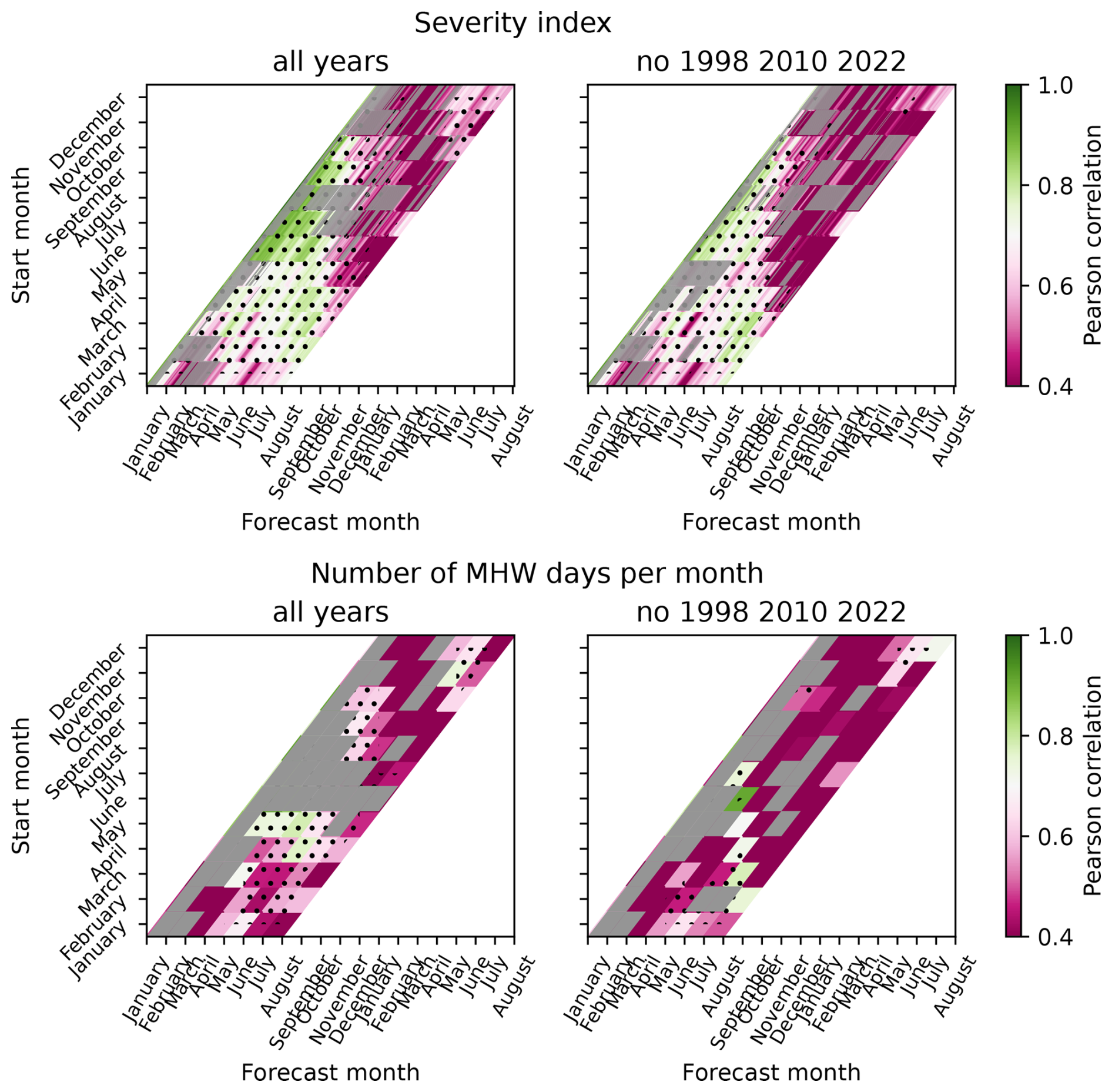
Figure 8 Deterministic skill of the severity index (top row) and the number of MHW days per month (bottom row) as a function of both lead time and start month of the forecast (y-axis). The x-axis represents the forecast target date. Grey areas indicate that persistence has a higher skill than the forecast. Dots indicate that the correlation is significant (p-value < 0.05).

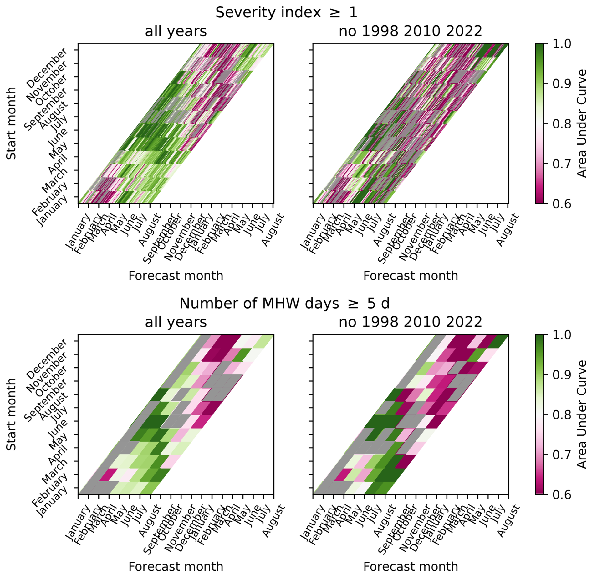
Figure 9 Probabilistic skill of the severity index (top row) and the number of MHW days per month (bottom row) as a function of both lead time and start month of the forecast (y-axis). Grey areas indicate that persistence has a higher skill than the forecast.

3.4 Influence of the start month

Here we evaluate the seasonality of the forecast skill in the Météo-france forecast System 8, and thus compute it for each start month separately: for instance for january the skill is computed based on the 29 forecasts (1993–2018 + 2022–2024) initialized on 1 January of each year. We perform this computation for both deterministic (Fig. 8) and probabilistic (Fig. 9) skill, as well as an additional computation with the 3 “unusual years” (1998–2010–2022) removed (right columns in Figs. 8 and 9). As in the previous section, the skill is computed as a fonction of leadtime, and can here be interpreted as the forecast target date: all forecasts of the month of august, for instance, are aligned vertically, whether they started 1 month earlier (i.e. with a leadtime of 1 month) or 6 months earlier (i.e. with a leadtime of 6 months).

These results show that the previous sections, where all starting months were aggregated, hide strong variability. For both the probabilistic and deterministic approaches, forecasts targeting the cold season (June–September) generally have a much higher skill than forecasts targeting the warm season (October–March), even at very long lead times (up to 7 months, see for instance forecasts targeting August and starting in February in Figs. 8a and 9a–c). This patterns also illustrates the counterintuitive result that skill can sometimes increase with leadtime. For instance for a forecast starting in February the skill is very low for the first few months, which target the warm season (leadtime 1–3 months, i.e. February–April), but becomes higher at longer leadtimes that target the cold season (leadtime 6–7 months, i.e. July–August). The opposite occurs for forecasts that start during the cold season, with initially very high skill that decreases sharply after September/October. Importantly, the forecasts are generally better than the reference persistence forecast (indicated by grey areas in Figs. 8 and 9).

This seasonal difference in skill is likely caused by the higher MHW variability in the warm season, which typically has shorter MHWs every year, in contrast with the cold season. Indeed, these seasonal patterns in skill occur every year, even when the 3 atypical years with very long MHWs (in 1998, 2020 and 2022) are removed from the skill assessment (right column in Figs. 8 and 9).

3.5 Forecasting the triggering and ending of MHWs

We now investigate whether the Météo-france forecast System 8 is able to predict the transitions from normal conditions to a MHW (the triggering of the next MHW) and from an ongoing MHW to normal conditions (the end of that MHW). Here MHWs are detected within a probabilistic framework: the forecast is considered in a MHW state if more than 20 % of the members are in a MHW state (category≥1), which is the optimal decision threshold identified with the ROC curve (Fig. 6 and discussion above). We separate the forecasts that start in normal conditions (Fig. 10a) and the forecasts that start in a MHW (Fig. 10b), and for each case we compute the duration (number of days) until the transition to another MHW state occurs. We then evaluate the correlation between the observations (x-axis) and in the forecast (y-axis). The position of points above or below the diagonal indicates whether the forecast has overestimated or underestimated the date of this transition.

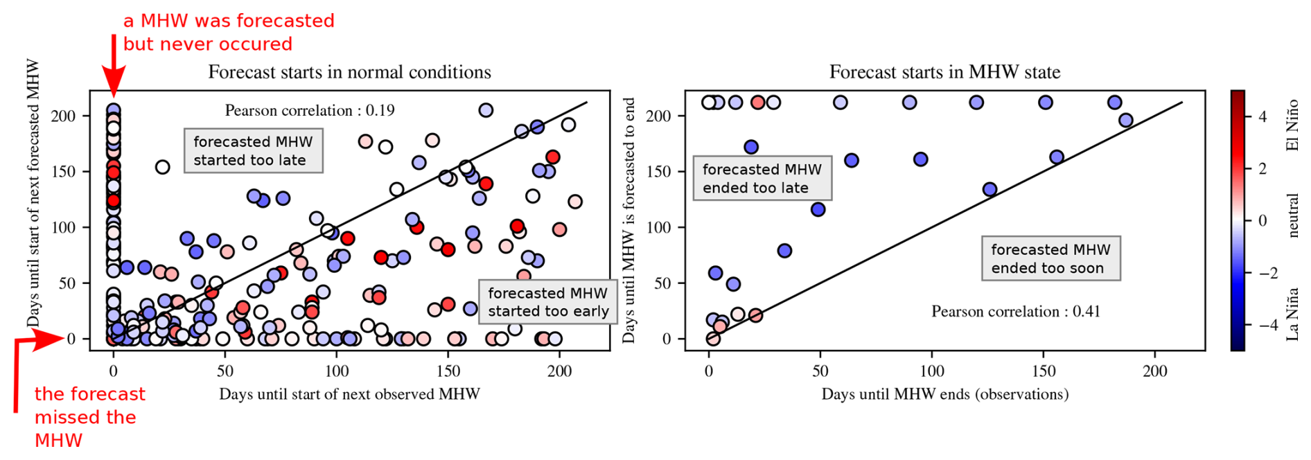
Figure 10 Left panel: number of days until the next MHW starts, as observed (x-axis) and forecasted (y-axis) for forecasts which start in normal conditions (no MHW). Right panel: number of days until the current MHW ends, as observed (x-axis) and forecasted (y-axis) for forecasts which start in a MHW. The color of the markers is the average ONI (Oceanic Nino Index) for the duration of the forecast; blue indicates that the forecast was primarily during a Nina phase and red during a Nino phase. The occurrence of a MHW in the forecast was determined using a probabilistic approach with a threshold of 20 % (i.e., the forecast is in a MHW state if more than 20 % of members are in a MHW state).

We find that the forecast system is generally not very skilled at predicting these transitions, even at short leadtimes. The Pearson coefficient indicates weak correlations between forecast and observations for predictions of the start of the next MHW (0.19) and of the end of the ongoing MHW (0.41). When the forecast starts in normal conditions, it tends to predict that the next MHW will occur too early (majority of points below the diagonal in Fig. 10a), and there are many cases where it predicts a MHW that never occurs (points aligned vertically at 0), or completely misses the next MHW (points aligned horizontally at 0). Conversely, when the forecast starts in a MHW state, it tends to predict that the current MHW will last longer than observed (all points above the diagonal in Fig. 10b). However, it should be noted that some transitions are rather well forecasted many months in advance, particularly the end of MHWs during La Niña phases (blue points in Fig. 10).

Figure 11 Deterministic forecast skill in the South West Pacific (Météo-France System 8).

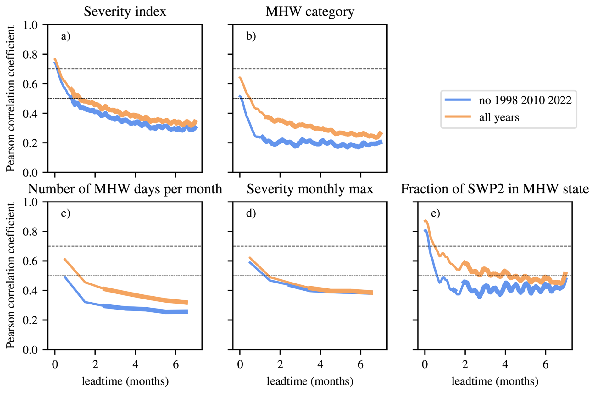
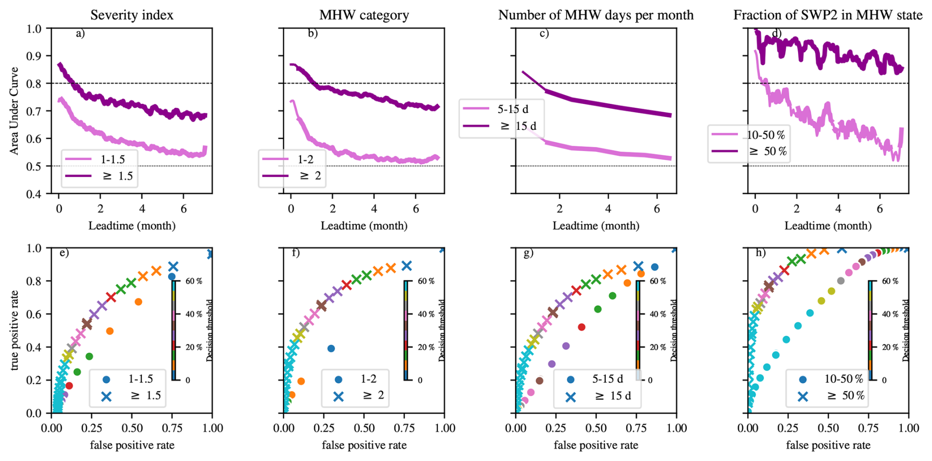
Figure 12 (a)–(d) Probabilistic forecast skill in the South West Pacific (Météo-France System 8). (e)–(h) Spatial average as a function of lead time. Bottom row: ROC curves (average of all lead times).

3.6 Widening the scope to the South West Pacific

Finally, we investigate if the conclusions reached in the previous sections for the relatively small area of the New Caledonia EEZ are also valid for the wider Southwest Pacific region, and find that this is the case (Figs. 11 and 12). We find (1) a decrease of the skill with leadtime, (2) an important role of the 3 key La Niña years for improving the forecast skill, (3) a better skill with a probabilistic approach compared to a deterministic approach, and (4) better predictability for intense, large-scale and longer MHWs. The results on the seasonality of skill (higher for the cold season) are also valid for this wider region (not shown). In addition, we found that the forecast skill is generally spatially uniform in the Southwest Pacific (Figs. A4–A6). A weak spatial gradient in the skill does emerge for some metrics and leadtimes, with higher skill in the northwest part of the domain (Figs. A4b–d and A6d). Thus, we conclude that the application of this framework to other close Pacific island nations (such as Fiji, Vanuatu, or Wallis and Futuna) would be worth exploring in a future study.

4 Discussion

4.1 Influence of drivers and mechanisms on the predictability of MHWs

We investigated three factors that could influence forecast skill: the spatio-temporal scale (MHWs defined at a specific day and point or for an entire region/period), the properties of MHWs (extreme or weak, in terms of intensity, duration and spatial extent) and the timing of MHWs (season and ENSO phase).

Previous studies have found that MHWs are more predictable in regions strongly affected by ENSO, like the tropical eastern Pacific (Jacox et al., 2022; De Boisséson and Balmaseda, 2024) or by ENSO teleconnections, like the Arabian sea (Koul et al., 2023). Here, we show that ENSO also affects the predictability of MHWs in the Southwest Pacific, where the influence of ENSO is more ambiguous as it combines with other modes of variability like the MJO (Dutheil et al., 2024) and smaller-scale intrinsic ocean variability (Cravatte et al., 2021).

Here in our historical record (1993–2024), we identified that long duration and large-scale MHWs around New Caledonia are associated with strong La Niña events during the austral winter (Fig. 3), consistent with previous global studies of MHW drivers (Holbrook et al., 2019; Sen Gupta et al., 2020). Since ENSO is the climate mode with the highest predictability at seasonal timescales (Ehsan et al., 2024), this suggests that these particular types of MHWs are easier to predict. Indeed, our probabilistic approach, which allowed us to differentiate between long, intense, large-scale MHWs and smaller events, concluded that the predictability of the former is higher (Fig. 6). This suggests that the high predictability of ENSO is responsible for the high predictability of these long, intense, large-scale MHWs (Hobday et al., 2023), likely through anomalous large-scale oceanic and atmospheric conditions influencing air-sea fluxes (Vogt et al., 2022; Bian et al., 2024). However, it should be noted that while forecast skill is generally higher in years affected by La Niña events (compare Figs. 6 and A9), the difference in predictability between the two types of events occurs in other years as well, suggesting that it is generated by a mechanism independent of ENSO. Similarly, the MJO is another climate mode of variability with some predictability at subseasonal timescales (Lim et al., 2018) known to influence MHWs (Dutheil et al., 2024; Gregory et al., 2024). However its influence on MHW predictability has received little attention so far (Wang et al., 2023).

These particular types of MHWs should not overshadow the much more numerous smaller scale MHWs, which may have a significant cumulated impact despite being individually weaker (Lal et al., 2026; Pietri et al., 2021). While anomalous air-sea fluxes linked to synoptic atmospheric events may play a role in the generation of such smaller MHWs, their poor predictability is consistent with ocean advection as their main driver, as previous studies have suggested for other regions (Bian et al., 2024; Mogollón et al., 2025). Indeed, ocean advection is largely chaotic in the study region (Cravatte et al., 2021) and thus would be more difficult to forecast.

However, we also found that the scale at which MHWs are defined does not influence skill: contrary to our expectations, there was no improvement in skill when we defined metrics aggregated over a certain region or time period, thus ignoring information about the exact location of a MHW within this region or the exact date of occurrence within that period. This could be explained in two ways: either the small scales and the large scales are equally well-predicted, or MHWs generation is dominated by slower processes because of the thermal inertia of the ocean (Holbrook et al., 2020). The latter interpretation was favored by Jacox et al. (2022), who noted that “The consistency between the monthly and daily forecast skill is not surprising given that MHWs defined with daily data are still strongly driven by low frequency variability.” (see their supplementary section) We recommend that future research should focus on identifying the drivers of different types of MHWs in order to understand their sources of predictability.

4.2 Implications for operational use: is the forecast useful and useable?

Spillman et al. (2025) proposed a three-step framework to help transfer MHW forecast information from researchers to stakeholders, which include ecosystem managers, marine industries like aquaculture or tourism, and indirect users like supermarkets or insurance companies. The first step is the usefulness of the forecast (having the appropriate model type, resolution, and domain, with model skill verified against observations), the second step is the useability (is the skill on timescales relevant to decision making, interpretable by end users, and delivered in a practical format?) and the third step is ensuring that the forecast is used (communication and user engagement). Here we discuss some aspects of our results relevant to the first two questions that can serve as the basis for co-constructing operational bulletins with marine stakeholders.

We performed our analysis with two seasonal forecasting systems (Météo-France System 8 MF8 and ECMWF SEAS5) that have similar configurations, especially for the representation of the ocean: both use the NEMO model at an eddy-permitting resolution ($\mathrm{1}/\mathrm{4}$°), although the products are distributed by Copernicus interpolated on a coarser 1° grid. However, NEMO is coupled with a different atmospheric model for each system and the initialization schemes are different. We focused on the scale of an EEZ, choosing New Caledonia as an example, because it represents a coherent unit, administered by a relatively small number of institutions (the New Caledonia government and three provinces) and consistent with the area of operations for many stakeholders (such as the local longline tuna fishery, tourist operators and conservation managers). While a higher resolution would result in a better representation of physical processes, particularly near the coast, there are currently no such operational products available, although Mercator Ocean International is in the process of expanding their 10 d forecast to subseasonal timescales (pers. comm.). The skill was evaluated by comparing the hindcasts against reanalyses that use the same ocean model (NEMO) at different resolutions: $\mathrm{1}/\mathrm{12}$° for Glorys, used to evaluate MF8 and $\mathrm{1}/\mathrm{4}$° for ORAS5, used to evaluate SEAS5. The discrepancy in resolutions could explain why SEAS5 performs better than MF8: the former resolves the same physical processes as its reference ORAS5 while the latter is lacking finescale processes that are resolved by the reference Glorys. Indeed, model resolution was shown to strongly influence MHW characteristics (Pilo et al., 2019), especially in highly dynamic region like the South West Pacific (Keppler et al., 2018).

Regarding the composition of bulletins, we first recommend using probabilistic metrics because they tend to be more skilled. However, this increased skill will need to be balanced with their relative complexity, compared with the more simple deterministic metrics, in order to create a forecast suitable for their intended audience and their level of familiarity with such forecasts. Previously, probabilistic metrics have been used to detect the occurrence of MHWs (Jacox et al., 2022; Hu et al., 2025), while deterministic metrics have been used to describe their properties in more detail (McAdam et al., 2023). Conversely, De Boisséson and Balmaseda (2024) and Smith and Spillman (2024) assessed both types of metrics simultaneously and found that they have equivalent levels of skill. They concluded that an operational forecast should supply them both, as they provide complementary information. Here, through the use of multiple metrics and value thresholds, we were able to extract probabilistic information on the occurence of MHWs with different properties and at different spatial and temporal scales. Among the deterministic metrics, we found varying levels of skill: the monthly maximum of severity performs best, and the category worse, with other metrics (daily severity, number of MHW days per month and surface fraction in MHW state) falling in between. Among the probabilistic metrics (based on severity, category, number of MHW days per month and surface fraction) we found comparable levels of skill. These metrics may be suitable for different users depending on their exact needs. Since the forecast skill of the most extreme MHWs is higher than that of milder MHWs (covering a smaller area, shorter and less intense), an early warning system based on these more extreme MHWs would be both more reliable and more relevant, since they usually have the largest impacts.

Second, we recommend raising a “MHW alert” when an optimal decision threshold of 20 % is reached (i.e., when more than 20 % of the members predict a MHW) in order to maximize hits and minimize false alarms. This choice is supported by the shape of the ROC curves (Fig. 6), and is also intuitive: 20 % is a round number and corresponds to a doubling of the climatological probability of a MHW (which the 90th percentile constrains at 10 %). The climatological probabilities of all the MHW events considered (for instance a MHW of category 2, or covering more than 50 % of the EEZ) needs to be made available along with the forecasts to provide context to guide their interpretation (Tables A1–A4). Also, for simplicity, we recommend a single value for all metrics and leadtimes in both forecast systems, even though the 20 % threshold will perform better in some cases than others. In practice, this means that an alert should be raised if more than 20 % of members predict a MHW. This value may seem low but it should be remembered that MHWs are rare events. Any probability higher than the climatological probability (about 10 % by design with the choice of a 90th percentile threshold, see Fig. 3e) can be considered an increase in risk. We used this decision threshold of 20 % to define an additional metric of direct relevance to stakeholders: the date of the next MHW when the forecast is started in normal conditions, which could be used in early warning systems, and the end date when the forecast is started during a MHW, which could be used to plan recovery efforts. Unfortunately, we found a low skill for both these metrics in the Météo-France forecast System 8 (Fig. 10). The apparent discrepancy between this low skill for the start date and the high probabilistic skill can be explained by the fact that the start date metric gives an equal weight to all MHWs. On the contrary, a long MHW represents many time steps and will weigh more in the computation of probabilistic skill metrics than a short MHW. Thus, the few very long and very large MHWs (occurring in the austral winter during La Niña years) that are well predicted drive an increase in probabilistic skill, while the many ill-predicted shorter summer MHWs have a low influence on the AUC. If used for management, the use of these metrics about the start/end of MHWs will overestimate the risks, predicting that the next MHW will arrive too soon, or that the current MHW will last too long. This could cause many false alarms and result in a loss of credibility in the forecasts. Thus the usefulness of the forecast for a particular user will depend on the application and on the sensibility to false alarms. For instance if the forecast predicts a very long summer MHW, reef managers might be able to plan for continued monitoring of bleaching by requesting resources such as ships, divers or planes, and then cancel these efforts if the MHW stops earlier than expected (Maynard et al., 2009). On the other hand, repeated false alarms might endanger the profitability of marine industries such as aquaculture if they are associated with investments that never pay off (Hartog et al., 2023).

Third, since we found similar levels of skill when we performed the verification for each grid-point vs for averages in the EEZ, the presentation of the forecasts (in maps or timeseries) can be decided according to the preferences of stakeholders.

Regarding the interpretation of bulletins, we found that the skill of forecasts is highly variable in time at both seasonal and interannual scales. First, MHW forecasts targeting the warm season have lower skill than forecasts targeting the cold season. This seasonal pattern of skill has not previously been described, although some studies revealed that skill tends to be better in winter (De Boisséson and Balmaseda, 2024; Smith and Spillman, 2024). Unfortunately, summer MHWs predictions would be more useful for marine stakeholders, because they are associated with the largest impacts as temperatures can exceed the upper thermal tolerance limit of organisms (Wernberg et al., 2025). For instance coral bleaching, one of the most visible impacts of MHWs, strictly occurs during summer. For this reason, many skill evaluation focus on the summer MHWs (McAdam et al., 2023; Koul et al., 2023) or on bleaching metrics (Liu et al., 2018; Spillman and Smith, 2021). However it should be kept in mind that winter MHWs also have impacts and could benefit from reliable forecasting, for instance for monitoring invasive species (Atkinson et al., 2020) or HAB (harmful algal bloom). Second, forecasts coinciding with strong La Niña have more skill than forecasts made during neutral or El Niño phases. Thus, the leadtime at which a forecast can be considered skillful is highly variable, depending on the metric of interest, but also the season and the ENSO phase, ranging from virtually no skill even at short leadtimes (e.g. for deterministic metrics in Austral summer) to sustained skill 6 months in advance (e.g. probabilistic skill in Austral winter). The level of interannual variability could also inform the choice of metrics, as it might be easier to communicate forecasts based on metrics that have the same level of skill every year (such as the severity monthly maximum) We stress that information on skill should be an integral part of bulletins, as it can influence whether the forecast is acted upon or not, in accordance with the risk-profile of each stakeholder. For instance some stakeholders may want to adopt a precautionary position and take action even if the forecast has a high uncertainty, while others may want to minimize false alarms by only acting on skilled predictions (i.e., for winter MHWs during La Niña).

5 Conclusions

We evaluated the skill of the seasonal forecasts from Météo-France System 8 and ECMWF SEAS5, specifically targeting MHWs in the South West Pacific ocean. To go beyond simply predicting the occurence of MHWs, we provided a range of metrics that can give a complete description of the exposure to MHWs, defined in terms of intensity, duration and spatial extent, as well as the date of the transitions between a normal state and a MHW state. We also investigated the factors that influence the skill, in order to guide the interpretation by identifying situations where more confidence can be placed in the forecasts. We found that the level of skill is highly variable and depends on the type of approach (deterministic or probabilistic), the targeted metric, the properties of the MHWs (duration, spatial extent, severity), the season and ENSO state. While the SEAS5 forecasts have an overall higher skill than Météo-France System 8, these results are robust across the two forecast systems. Ongoing and future work aim to improve the usefulness of the forecasts by combining social science studies to identify the vulnerabilities of local communities with the exploration of different forecasting systems such as a higher resolution model or machine learning approaches. In order to make sure that the forecasts are both useable and used, the co-construction of the bulletins with local stakeholders is essential, as is a close collaboration between academics and operational centers to efficiently produce and distribute these bulletins. Here we investigated surface MHWs defined based on the SST because no other ocean variable is commonly distributed by seasonal forecasting centers. However, this superficial and narrow view should be extended to include the vertical dimension and additional variables. Recent studies have shown that MHWs are not vertically homogeneous (Fragkopoulou et al., 2023; Zhang et al., 2023; Malan et al., 2025). Zhang et al. (2023) identified four types of vertical structures (shallow, subsurface-reversed, subsurface-intensified and deep MHWs) that are influenced by different ocean processes, and are all found in equal proportion in our region (the Southwest Pacific). They found that subsurface-intensified MHWs are more heavily influenced by ENSO than the other types, which suggests that they may be more predictable than surface MHWs. Similarly, deep MHWs may be more predictable than surface MHWs because they are less influenced by chaotic atmospheric processes. Indeed, using heat content in the upper 40 m of the water column from the Euro-Mediterranean Centre on Climate Change, McAdam et al. (2023) showed that subsurface MHWs are easier to predict that surface MHWs for large parts of the global ocean. Multiple studies have shown that extreme values of variables other than temperature are also important drivers of ecosystem health (Gruber et al., 2021; Le-Grix et al., 2023). Some forecast products already include ocean variables such as alkalinity, Dissolved Inorganic Carbon, or Chlorophyll (Siedlecki et al., 2023), but extreme events are not yet included although they can have skill at long leadtimes – for instance extreme acidification events (Mogen et al., 2023). Thus, forecast products should endeavour to include MHWs for both the surface and subsurface, as well as extreme events of other ecosystem stressors and compound events, in order to give a full description of the upcoming state of the ocean.

Appendix A: Use of the ROC for rare events

The AUC is base-rate independent, which means that it doesn't overestimate the skill of the model for rare events. This is a significant advantage compared with other commonly used metrics such as the Brier score. We also opted not to use the SEDI, a score designed specifically for rare events (Ferro and Stephenson, 2011). While the SEDI possesses many properties interesting to finely describe the skill of the model, its computation introduces some arbitrary choices which make interpreting and communicating results more difficult. Therefore, we focus in this paper on AUC and ROC.

A common issue with using the AUC for rare events is that the points used to construct the ROC can cluster toward the lower left corner when the incremental decision thresholds are not well suited to the baserate (Ben Bouallègue and Richardson, 2022). To avoid this, we ensured that the ROC had a correct shape by including enough decision thresholds in the lower range (for instance between 0 % and 10 %). We also selected value thresholds to define binary events with reasonable baserates. One consequence is that we use different thresholds for intense exposure based on the category and the severity. The occurence of a MHW category higher than 2 is higher than occurence of a severity higher than 2 because the entire MHW is classified as category 2 even if the treshold is exceeded for just 1 d. However, this occurence is still too low to generate a well-shaped ROC curve (note the points clustered in the lower left corner in Fig. 6f); this issue could be solved either by increasing the number of members in the ensemble or by including a secondary decision variable as suggested in (Ben Bouallègue and Richardson, 2022). To avoid this problem with the severity, which contrary to the category is a continuous variable, we were able to lower the threshold to 1.5 to increase the baserate and generate a correct ROC curve.

Thus, all the binary events evaluated have similar baserates, typically between 5 % and 15 % (Figs. A2 and A3, and Tables A1–A4). These baserates are high enough so that another common criticism of the AUC – its inapplicability to imbalanced datasets (Saito and Rehmsmeier, 2015) – is not relevant here.

Table A1 Climatological frequency in the GLORYS reanalysis of two levels of intensity exposure defined with the MHW category for the period 1993–2024, averaged in the New Caledonia EEZ and in the South West Pacific ocean.

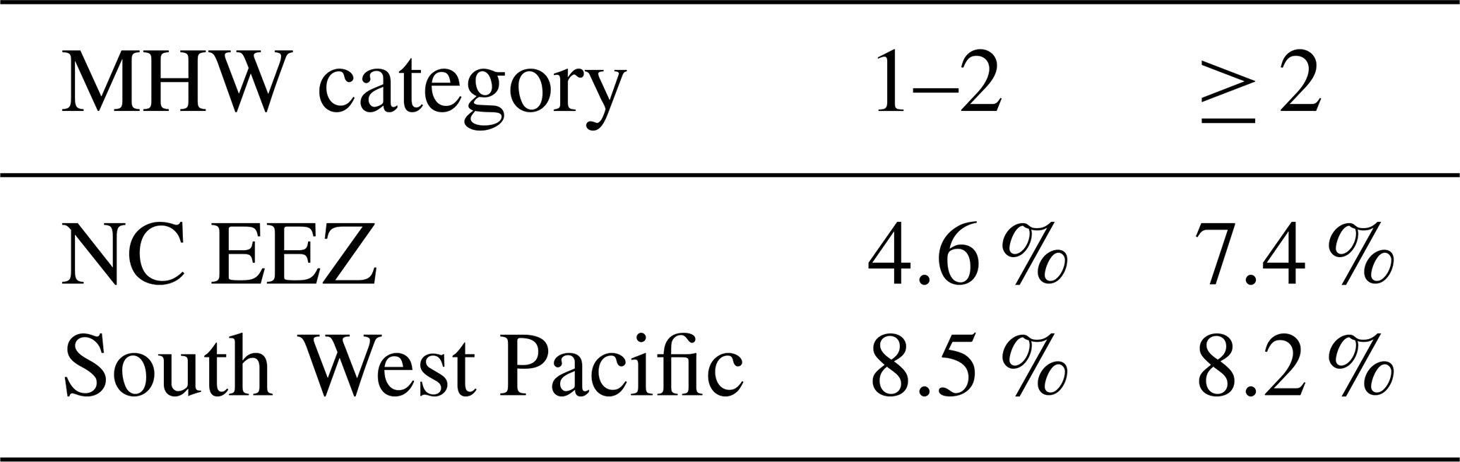
Table A2 Climatological frequency in the GLORYS reanalysis of two levels of intensity exposure defined with the MHW severity for the period 1993–2024, averaged in the New Caledonia EEZ and in the South West Pacific ocean.

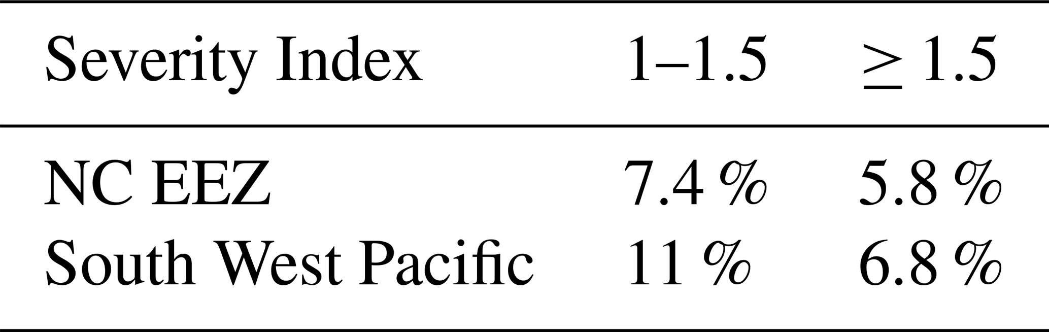
Table A3 Climatological frequency in the GLORYS reanalysis of two levels of duration exposure defined with the number of MHW days per month for the period 1993–2024, averaged in the New Caledonia EEZ and in the South West Pacific ocean.

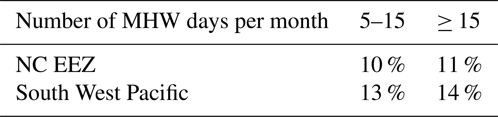
Table A4 Climatological probability (1993–2024) in the GLORYS reanalysis of two levels of spatial cover exposure.

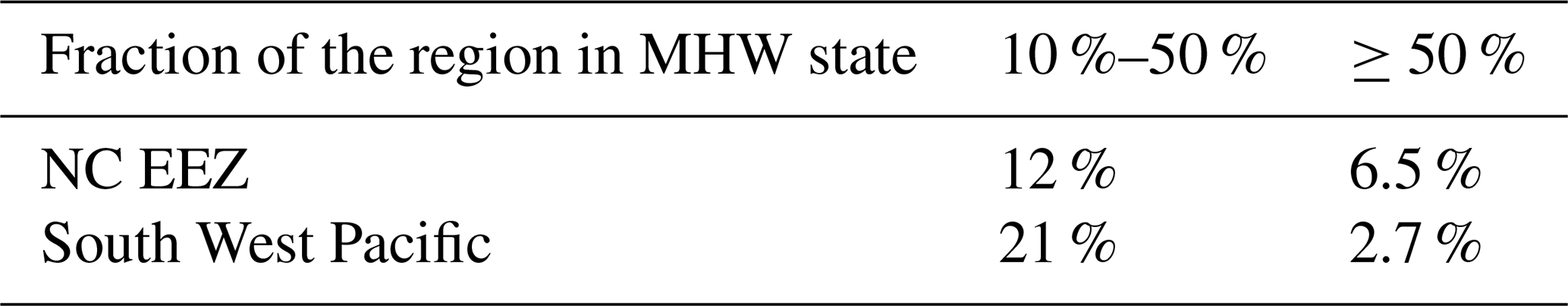
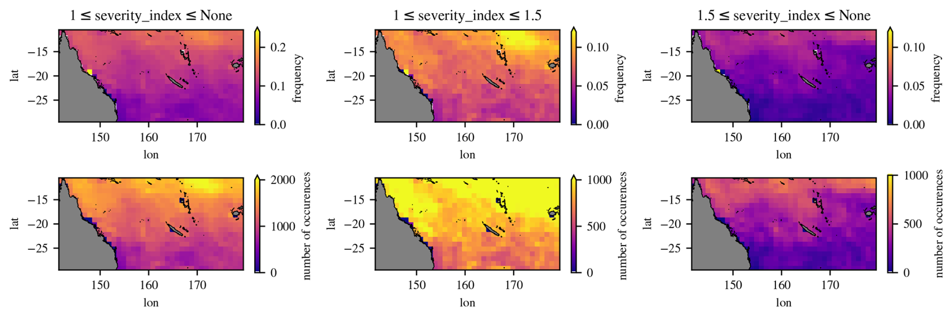
Figure A1 Climatological frequency and number of occurences of MHW in the GLORYS reanalysis for the period 1993–2024. Each column corresponds to a binary event derived from the MHW severity index: all (severity_index≥1, first column), moderate ($\mathrm{1}\le \mathrm{severity}\mathrm{index}\le \mathrm{1.5}$, second column) and severe (severity  index≥1.5, third column). The bottom row shows the number of days fulfilling the condition, in the 32 years historical record. The top row shows the climatological probability (or baserate), ie the number of days fulfilling the condition divided by the total number of days.

Figure A2 Climatological frequency and number of occurences of MHW in the GLORYS reanalysis for the period 1993–2024. Each column corresponds to a binary event derived from the MHW category: all (category≥1, first column), moderate ($\mathrm{1}\le \mathrm{category}\le \mathrm{2}$, second column) and severe (category≥2, third column). The bottom row shows the number of days fulfilling the condition, in the 32 years historical record. The top row shows the climatological probability (or baserate), ie the number of days fulfilling the condition divided by the total number of days.

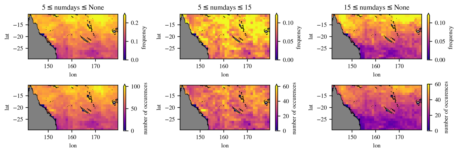
Figure A3 Climatological frequency and number of occurences of MHW in the GLORYS reanalysis for the period 1993–2024. Each column corresponds to a binary event derived from the number of MHW days per month “numdays”: all (numdays≥5, first column), moderate ($\mathrm{5}\le \mathrm{numdays}\le \mathrm{15}$, second column) and severe (numdays≥15, third column). The bottom row shows the number of months fulfilling the condition, in the 32 years historical record. The top row shows the climatological probability (or baserate), ie the number of months fulfilling the condition divided by the total number of months.

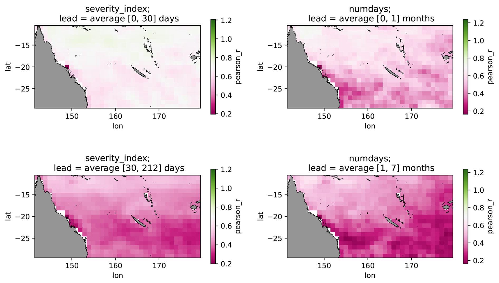
Figure A4 Map of deterministic skill (Pearson correlation) for two leadtime ranges: short (top row) and long (bottom row). Left column: severity index. Right column: number of MHW days per month.

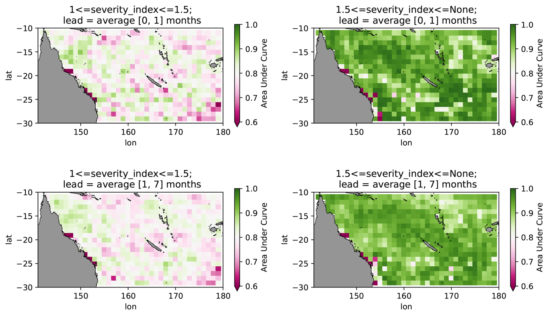
Figure A5 Map of probabilistic skill (AUC) of the severity index for two leadtime ranges: short (top row) and long (bottom row). Left column: moderate exposure. Right column: severe exposure.

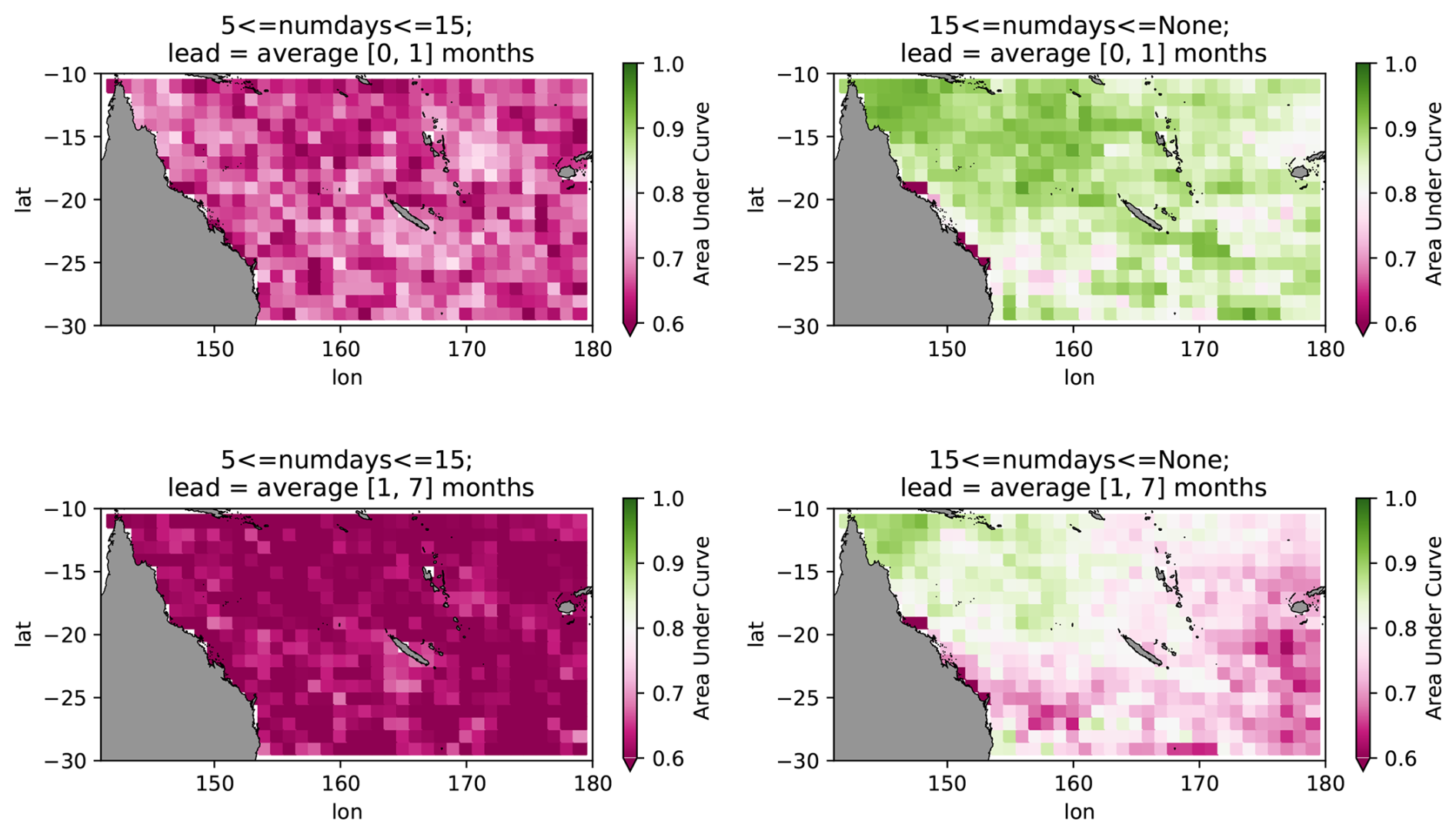
Figure A6 Map of probabilistic skill (AUC) of the number of MHW days per month (“numdays”) for two leadtime ranges: short (top row) and long (bottom row). Left column: moderate exposure. Right column: high exposure.

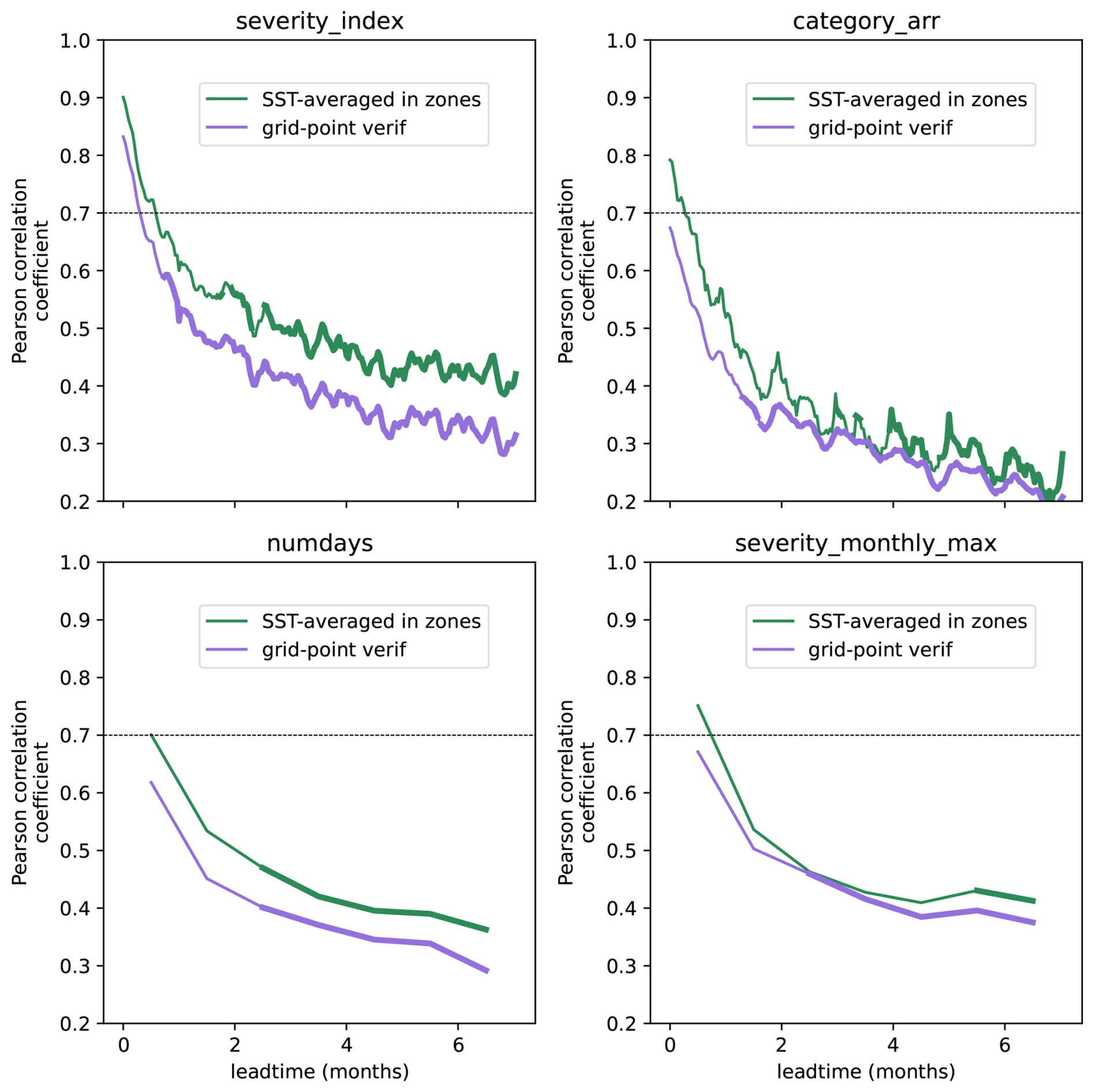
Figure A7 Comparison of deterministic skill (Pearson correlation) of 4 MHW metrics for two spatial approaches each: (green) the SST is averaged in the region of interest (here the NC EEZ) and then the MHWs are detected and the verifaction performed, producing a single value for the region; (purple) the MHW detection and verification are performed for each grid point (cf the skill maps Fig. A4), then the skill metric is averaged in the region of interest.

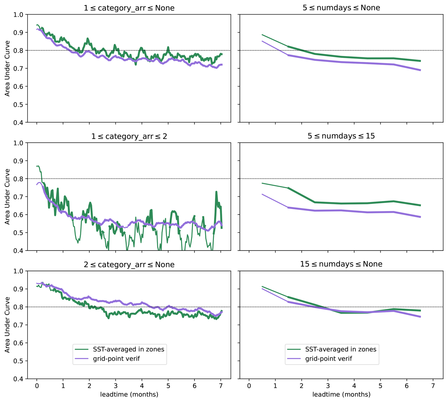
Figure A8 Comparison of probabilistic skill (AUC) of the category and number of MHW days per month for two spatial approaches: (green) the SST is averaged in the region of interest (here the NC EEZ) and then the MHWs are detected and the verifaction performed, producing a single value for the region; (purple) the MHW detection and verification are performed for each grid point (cf the skill maps Figs. A6 and A5), then the skill metric is averaged in the region of interest.

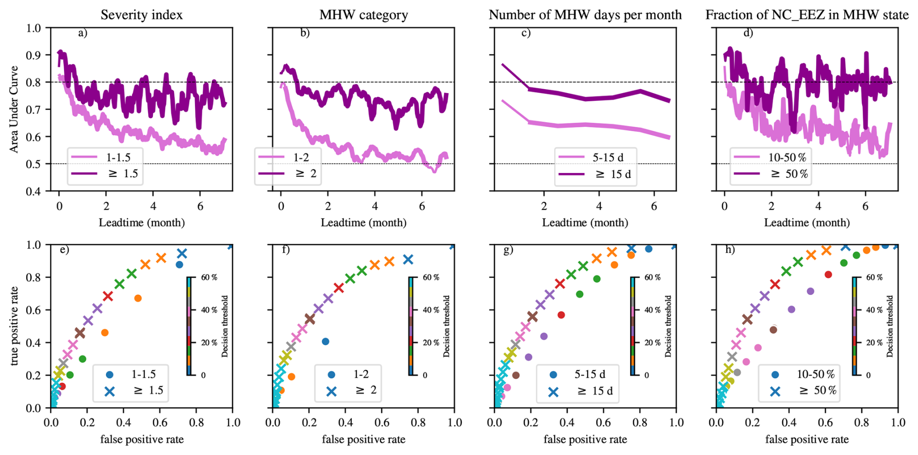
Figure A9 Probabilistic skill: same as in Fig. 4 but computed without the 3 strong La Niña years (1998–2010–2022).

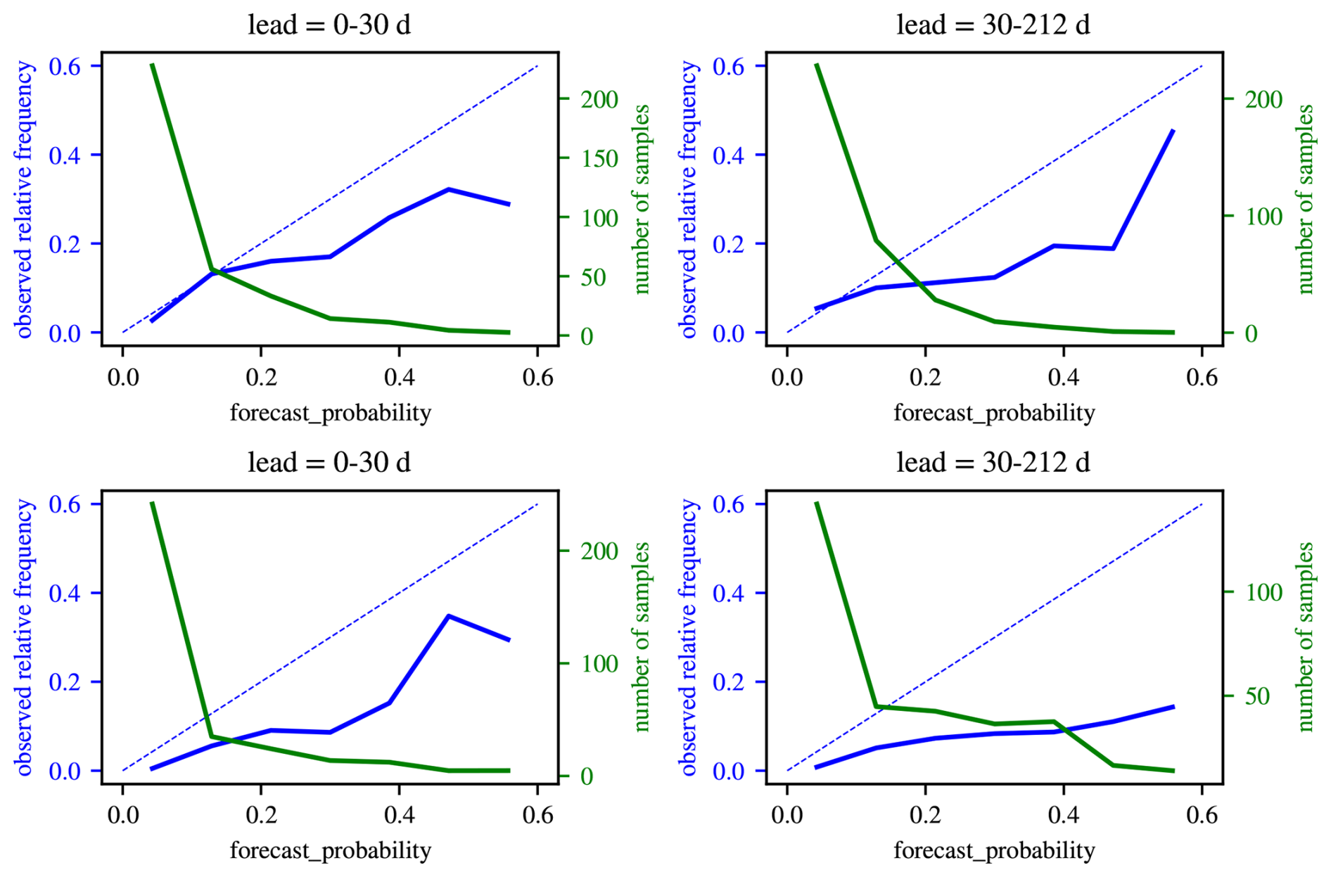
Figure A10 Reliability diagram (blue line) for the two severity levels of exposure: low (top row, $\mathrm{1}\le \mathrm{severity}\le \mathrm{1.5}$) and high (bottom row, (severity≥1.5). In each probability bin (x-axis), the blue line shows the observed frequency among all days where the forecast predicted this probability. The diagonal represents a perfectly calibrated forecast. Since the blue line is below the diagonal, the diagram shows that the forecast (here Météo-France System 8) usually overpredicts MHW events. The green line shows the number of samples in each probability bin.

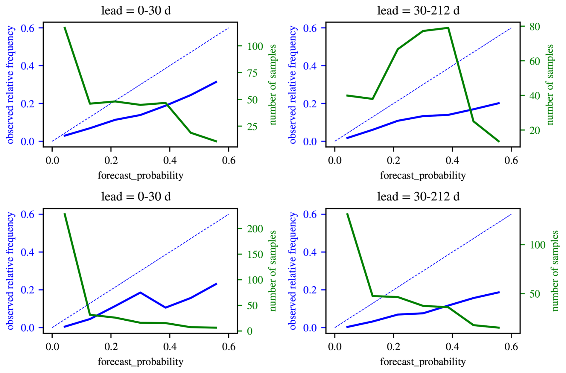
Figure A11 Same as Fig. A10, but for the two surface fraction levels of exposure: low (top row, $\mathrm{0.1}\le \mathrm{frac}\le \mathrm{0.5}$) and high (bottom row, (frac≥0.5). Since the blue line is below the diagonal, the diagram shows that the forecast (here Météo-France System 8) usually overpredicts MHW events.

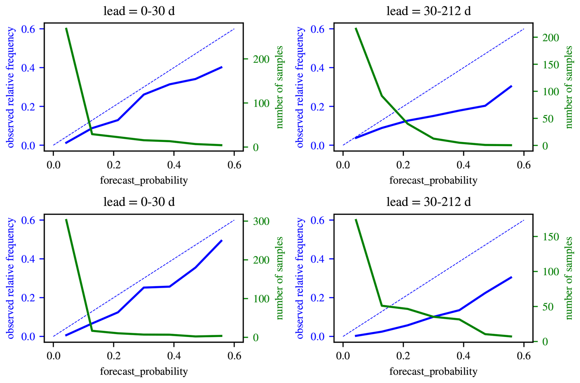
Figure A12 Same as Fig. A10, but for the ECMWF SEAS5 system. The forecast is better calibrated than Météo-France System 8, but also overpredicts MHW events.

Figure A13 Same as Fig. A11, but for the ECMWF SEAS5 system. The forecast is better calibrated than Météo-France System 8, but also overpredicts MHW events.