the Creative Commons Attribution 4.0 License.
the Creative Commons Attribution 4.0 License.
 | 22 Jun 2026
Estuarine mixing
Knut Klingbeil
Xiangyu Li
Lloyd Reese
W. Rockwell Geyer
This review paper presents, explains and discusses major aspects of estuarine mixing which is defined as the destruction of salinity variance. Due to the large amounts of brackish water in estuaries produced by mixing of fresh river discharge and salty ocean water, mixing is one major characteristic of what is an estuary. In this review, mixing is quantified locally as well as on estuary-wide scales. Diagnostics of integrated mixing are given for estuarine volumes bounded by transects as well as isohalines (surfaces of constant salinity) moving with the flow. It is shown how entrainment across a moving isohaline surface depends on gradients of turbulent salt flux and mixing per salinity class. Various relations are derived that link estuarine salt mixing to other estuarine properties such as the freshwater discharge and the bulk estuarine circulation. For estuaries bounded towards the ocean by a fixed transect, the Knudsen mixing law is explained, where estuarine mixing is the product of the Knudsen salinities of inflowing and outflowing water masses and the river discharge. When the estuarine volume is bounded by a moving isohaline surface of salinity S, mixing inside the estuary is simply the product of S2 and the river discharge. Major processes that drive estuarine mixing are presented on various time scales (tidal, fortnightly, weather and discharge time scales) and spatial scales (channel-shoal interaction, mixing fronts). As underlying methods for the quantification of mixing, observational concepts, as well as numerical modelling methods such as consistent turbulence closure modelling and numerical mixing analyses are presented. As an outlook, some future perspectives are sketched. Many of the concepts presented in this review are illustrated using simulation results from a numerical model setup of the Elbe River estuary.
- Article
(9319 KB) - Full-text XML
- BibTeX
- EndNote


Estuaries are semi-enclosed coastal water bodies where riverine freshwater run-off from land is mixed with offshore salty ocean water to produce brackish water masses of intermediate salinities which are ejected offshore into the coastal ocean. In this sense, estuaries can be characterised as mixing machines (MacCready and Banas, 2011; Wang et al., 2017) with mixing rates far greater than in other parts of the ocean. Salt is the most characteristic constituent that is mixed in estuaries, because of (i) its significantly different concentration between rivers (typically <0.5 g kg−1) and the adjacent ocean (typically >30 g kg−1) and (ii) its inert character with no internal sinks and sources and no fluxes through the surface and the bottom. In addition to salt, there is a number of further properties, e.g., nutrients and pollutants, that are distinct between rivers and the ocean and which can be mixed in estuaries. This makes mixing a fundamental process in estuaries. We therefore follow here the definition of an estuary by Pritchard (1967) who stated An estuary is a semi-enclosed coastal body of water which has a free connection with the open sea and within which sea water is measurably diluted with fresh water derived from land drainage. Instead of diluted we would prefer to say mixed, which effectively has the same meaning but highlights mixing as the defining process of estuaries. Water bodies that follow this principle are classical estuaries in the sense that their functioning is based on a net freshwater water supply. The contrasting case is given by inverse estuaries that are based on a net freshwater deficit due to evaporation, leading to the export of hypersaline water masses. The present review focusses on classical estuaries (in the following just denoted as estuaries for simplicity), whereas inverse estuaries are only occasionally discussed as contrasting systems. Fundamental concepts of estuaries and estuarine circulation have already been covered by previous reviews (MacCready and Geyer, 2010; Geyer and MacCready, 2014), such that we here focus on mixing in estuaries and its physical and ecological consequences.
Much of the estuarine literature focusses on mixing, starting with Knudsen’s classic paper (Knudsen, 1900), in which he states: As the freshwater spreads out over the seawater it mixes with it so that the salinity of the surface increases seawards (translation by Burchard et al., 2018a). Fischer’s review (Fischer, 1976) is entitled Mixing and dispersion in estuaries, highlighting its fundamental importance. Notwithstanding the attention focused on mixing throughout the estuarine literature, the actual meaning of the term mixing has often been vague or ambiguous: everyone is familiar with mixing via the daily-life experience of pouring milk into a cup of tea and using a tea spoon to mix it. However, amid the complex and multi-scale processes in estuaries, that simple concept is overwhelmed by consideration of larger scale processes associated with turbulence, shear dispersion and buoyancy flux. Turbulence, diffusion, dispersion, buoyancy flux and mixing are often loosely treated as synonyms, leading to confusion as to what we mean by mixing.
In this review, we come back to mixing in a cup (or glass beaker), or more precisely to the thermodynamic definition of mixing, which is the destruction of variance of some scalar quantity (Gibbs, 1878). In the estuarine context, we focus on the destruction of salinity variance, which is defined in the oceanic turbulence literature as χs, due to the down-gradient diffusion of salt by molecular diffusivity
(Nash and Moum, 2002; Burchard and Rennau, 2008). In Eq. (1), κ is the molecular diffusivity of salt, is the turbulent salinity fluctuation, and square brackets denote Reynolds averaging (see Sect. 2.1 for details). In the turbulent environments of estuaries, this molecular process occurs at sub-millimetre scales, but it is the direct result of the turbulent and shearing motions acting on the salinity gradients at a wide range of scales extending all the way up to the horizontal dimensions of estuaries. It should be noted that the process of molecular mixing is irreversible inside the water body, such that χs≥0. Negative mixing or un-mixing can however occur at the sea surface when evaporation takes place (Yu, 2010; Klingbeil and Lorenz, 2025) or sea ice is produced due to freezing (Notz and Worster, 2009) and in desalination plants to extract freshwater from salt water (reverse osmosis, Kim et al., 2019). In numerical models, un-mixing can also occur due to discretisation errors of advection schemes (Henell et al., 2023). Maintaining the strict thermodynamic definition of mixing turns out to be a powerful approach to examining estuarine processes, because salinity variance can be defined locally, as is often done in the turbulence literature, as well as globally, at the overall scale of the estuary. We do not question the importance of other concepts, such as vertical buoyancy flux and horizontal dispersion, but in this review we retain the strict definition of mixing to explore the processes responsible for its occurrence in estuaries as well as its quantitative relationship to estuarine exchange flow.
Throughout this review, exemplary data from a numerical simulation of the Elbe River estuary in northern Germany are used to demonstrate the different mixing theories. The Elbe River estuary is an elongated meso-tidal estuary with one major discharge source at the landward end for which several studies of estuarine mixing have been carried out (Reese et al., 2024, 2026; Burchard et al., 2025). A brief introduction into the Elbe River estuary is given in Appendix C.
This review is structured as follows: After this introduction into the topic of estuarine mixing (Sect. 1), the existing theories on estuarine mixing are defined and discussed (Sect. 2). This section is structured into micro-structure mixing (Sect. 2.1) and parameterised mixing (Sect. 2.2), where Reynolds decomposition and turbulence closure assumptions are applied. The mixing definitions from Sect. 2 as well as the Total Exchange Flow analysis framework (Sect. 3.2) will be used in Sect. 3 (Estuarine Circulation and Mixing) to quantify mixing in entire estuaries. Before discussing estuarine mixing, we give a brief introduction to estuarine hydrodynamics (Sect. 3.1). For the mixing quantification, we first present the theory using fixed transects (Knudsen theories, see Sect. 3.3). Water Mass Transformation (WMT) theories (Sect. 3.4) are explained from which mixing laws for estuarine volumes bounded by isohaline surfaces as the seaward boundary are derived (Sect. 3.5). Section 3 concludes with some remarks on the relation between estuarine mixing and estuarine circulation (Sect. 3.6) and mixing of constituents other than salt (Sect. 3.7). While Sects. 2 and 3 focus on the definition and discussion of mixing, Sect. 4 gives examples for the most important estuarine processes that drive mixing. Those processes are related to single tides (Sect. 4.1.1), the spring-neap cycle (Sect. 4.1.2), time scales of river discharge and meteorological forcing (Sect. 4.1.3), channel-shoal interaction (Sect. 4.2.1) and mixing at fronts (Sect. 4.2.2). As methods to help quantifying mixing in estuaries, techniques to observe estuarine mixing are introduced (Sect. 5.1) and numerical modelling techniques are presented (Sect. 5.2), with a focus on turbulence closure modelling (Sect. 5.2.1) and numerical mixing (Sect. 5.2.2). Finally, some future perspectives are discussed in Sect. 6. The extensive appendix contains details about an analytic illustrative example for small-scale mixing (Appendix A), some key budget equations related to salinity variance (Appendix B), information about the Elbe River estuary model used to provide estuarine mixing examples (Appendix C), a derivation of the coordinate transformation of the vertical salinity equation (Appendix D), an explanation for the calibration of two-equation turbulence closure models (Appendix E), and derivations for the numerical mixing example (Appendix F). At the end of the Appendix, a table with the most important variables, their definitions, units and defining equations is presented (Table ).
While mixing occurs on the micro-scale only, its integral effects are most prominently effective on the large, estuarine scale. We therefore start our explanations with the quantification of local stirring and mixing. This will first be based on molecular diffusion on the micro-scale and Reynolds averaging on the macro-scale (Sect. 2.1) and then parameterised by means of turbulence closures as it would be calculated in numerical models of estuaries (Sect. 2.2).
2.1 Micro-structure mixing
Mixing of a tracer s (for which we use salinity here as an example) occurs at the micro-scale when tracer gradients are reduced by molecular diffusion, following the Fickian law,
where the Einstein summation convention has been applied. In Eq. (2), is the instantaneous tracer concentration with the Reynolds-averaged tracer concentration [s] and the fluctuating component , κ is the molecular diffusivity of salinity, and and are the horizontal and is the vertical velocity component. The terms in the brackets on the left hand side of Eq. (2) are the advective and the molecular diffusive fluxes, the divergence of which determines the change of the salinity distribution. This transport equation determines the salinity distribution on all scales ranging from the sub-millimetre scales of molecular diffusion to the global scales of meridional overturning circulation, including scales of estuarine mixing.
In turbulence theory, the Reynolds average (also called ensemble average) is defined as the average of an infinite number of macroscopically identical but microscopically different flow realisations, where the turbulent random fluctuations are averaged out (Lesieur, 2008). Consequently, . In estuarine physics, and similarly in most fields of larger-scale oceanography, the Reynolds-averaged rather than the instantaneous properties of the flow are considered. Field observations of tracer concentrations (e.g., from Conductivity-Temperature-Depth (CTD) probes) as well as numerical model results are supposed to represent Reynolds-averaged quantities. A continuity equation (incompressibility condition) is used in most ocean models:
applying to instantaneous and thus to Reynolds-averaged and fluctuating velocity fields. Using Eq. (2), a dynamic equation for the Reynolds-averaged salinity can be derived:
with the advective tracer flux [uj][s], the turbulent tracer flux and the diffusive tracer flux . Based on Eq. (2), it is also possible to derive an equation for the micro-structure tracer variance :
(see, e.g., Eq. (5) by Mellor and Yamada, 1974). In Eq. (5), Ps quantifies the production of micro-structure variance due to turbulent stirring (with the Reynolds-averaged tracer gradient vector ) and χs represents destruction of microstructure variance due to molecular mixing.
Multiplying Eq. (4) by 2[s] gives a transport equation for the square of the Reynolds-averaged tracer:
where on the right-hand side the stirring term Ps appears as a sink term besides a destruction term due to molecular diffusivity. In contrast to Eq. (5), where the destruction of micro-structure variance occurs due to molecular diffusivity acting on micro-structure gradients , in Eq. (6) the molecular diffusivity acts on the much smaller Reynolds-averaged gradient such that this term is generally negligible. This means that variance is first transferred from the Reynolds-averaged regime of Eq. (6) to the turbulent regime Eq. (5), where it is then dissipated. In turbulence closure modelling typically Ps=χs (see, e.g., Eq. (31) by Mellor and Yamada, 1974) is applied such that stirring equals mixing, following a local equilibrium assumption. More details on turbulence closure modelling suitable for estuaries are given in Sect. 5.2.
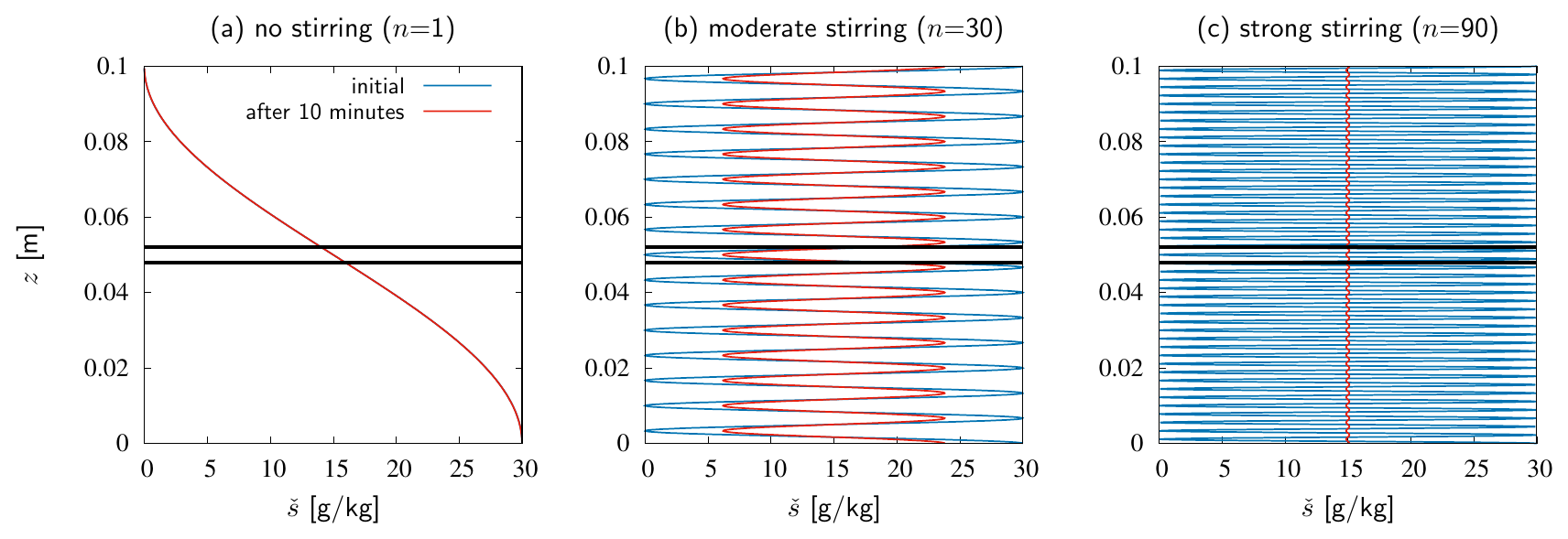
Figure 1Stirring and mixing in a glass beaker: (a) Evolution of salinity for the case of no stirring, (b) little stirring, and (c) strong stirring. The initial distribution after the stirring is shown as blue lines, and the distribution after 10 min is shown as red lines. The parameters for the problem are chosen as height of fluid inside the one-dimensional glass beaker D=0.1 m, and the molecular diffusivity of salinity, m2 s−1. The two black bars mark the area over which the local variance is estimated. More details are given in Appendix A .
In short: micro-structure tracer variance is produced by stirring Ps (increase of local micro-structure gradients due to turbulent eddies) and dissipated by mixing χs, while the divergence term on the left-hand side just spatially redistributes the micro-structure tracer variance. Note that the stirring term is twice the product of the turbulent flux times the Reynolds-averaged tracer gradient. The stirring term Ps is typically positive, since the Reynolds-averaged salinity gradient and the turbulent salt flux have opposite signs due to the generally down-gradient property of turbulent fluxes (classical exceptions occur in convective boundary layers, see e.g. Legay et al., 2025).
This can be explained by a laboratory experiment with salt mixing. A simple idealised model of this is given in Appendix A and results are shown in Fig. 1. After having carefully pumped saltwater of 30 g kg−1 underneath freshwater (with some continuous mixing), the local salinity variance is mostly low: sufficiently small control volumes would contain water with a small salinity range (Fig. 1a). Introduction of turbulence by means of a spoon will lead to stirring (increase of Ps), such that local control volumes (marked as the area between the two black bars in Fig. 1) will contain streaks of saltwater at various ranges, with sharp gradients between them, such that the local variance is increased. This is demonstrated as initial conditions for moderate stirring (Fig. 1b) and strong stirring (Fig. 1c). Now, mixing χs will be moderately or strongly enhanced due to the small (and constant) molecular diffusivity κ acting on the strong micro-scale gradients (which are squared in the mixing term). At the end of this process, the salt will be almost fully diluted in the water such that local variance becomes small, with and g kg−1. Further introduction of turbulence by a spoon will not lead to further stirring (and thus not to further mixing), because the tracer gradients have vanished.
In real estuaries, stirring typically occurs due to vertical shear instabilities driven by tidal flow, generating large eddies as shown in Figs. 17 and 18 in Sect. 5.1. Via the classical turbulence downward cascade, smaller and smaller eddies are generated such that finally mixing is enhanced at the smallest scales. Since estuaries are typically narrow and friction-dominated, horizontal instabilities on the submesoscale (McWilliams, 2016) play a minor role for stirring. An exception would be large fjord-type estuaries with weak tides such as the Baltic Sea (Chrysagi et al., 2021).
Direct in-situ measurements of salinity mixing χs are difficult to obtain due to the small value of the molecular salinity diffusivity of m2 s−1) and the consequently strong gradients at small scales, but successful attempts have been reported by Nash and Moum (2002) for locations on the continental shelf. According to these authors the salinity-gradient spectrum peaks at dissipative scales ten times smaller than the temperature-gradient spectrum, such that most salinity variance decay occurs in the sub-millimetre range. Therefore, and because of estuaries having generally higher levels of turbulence than continental shelves, direct observations of χs in estuaries are not feasible, and indirect observations are needed (see Sect. 5.1). Instead of using turbulence observations, mixing in estuaries is mostly studied by means of well-calibrated fine-resolution numerical models equipped with accurate numerical discretisations and physically based turbulence closures (Sect. 5.2).
2.2 Mixing at resolved local scales
Whereas the irreversible process of mixing happens at very small scales, the quantification of mixing is accomplished both in observations and in models through the application of turbulence closure assumptions (Mellor and Yamada, 1974; Peters and Bokhorst, 2001; Umlauf and Burchard, 2005). On the level of numerical ocean models, the turbulent fluxes are typically parameterised by means of the eddy diffusivity assumption, resulting in down-gradient turbulent tracer fluxes:
now using salinity s=[s] as Reynolds-averaged tracer concentration. In Eq. (7), Kh is the horizontal eddy diffusivity and Kv is the vertical eddy diffusivity. With this the Reynolds-averaged salinity budget equation Eq. (4) becomes:
showing that salinity changes are exclusively determined by the divergence of advective and turbulent fluxes. Note that in Eq. (8) molecular tracer fluxes have been neglected. With Eq. (7) the production of micro-structure variance due to stirring becomes
where in the last step stirring and mixing of micro-structure salinity variance are set equal, which is a typical assumption in turbulence closure modelling (see Sect. 2.1). The local variance decay χs is used as a local measure for the mixing of Reynolds-averaged salinity (Burchard and Rennau, 2008). This local equilibrium assumption is generally valid on the temporal and spatial scales that are resolved by numerical ocean models. In detail, χs appears as a sink term in both the salinity variance and salinity-square budgets. The corresponding derivation is shown in Appendix B.
In estuaries, the vertical term of the salinity variance decay Eq. (9) typically dominates over the horizontal terms due to the dominance of tidally-driven vertical shear (Li et al., 2024), such that we obtain
This is the case because in estuaries horizontal turbulent transports and their divergences are small compared to the vertical transports, with the consequence that in estuarine models the horizontal diffusion is often neglected in the parameterised salinity budget equation Eq. (8) as well as in the salinity variance equation Eq. (B1). Due to this dominance of vertical processes in estuaries, it is instructive to study the balance of the vertical variance,
for the vertical integral of which the following budget equation can be derived from Eq. (8), see Li et al. (2018) for details:
where η is the surface elevation. Equation (12) shows that the vertical variance balance is time-dependent and spatially variable. In contrast to the total salinity variance budget, the vertical salinity variance budget has source terms, the so-called horizontal straining terms, representing the conversion of horizontal variance (, where ) associated with the horizontal salinity gradient to vertical variance (Simpson et al., 1990). Note that horizontal straining is split into longitudinal straining and lateral straining (first and second term of horizontal straining, respectively) and can be a source (mainly during ebb straining) and a sink (mainly during flood straining) of vertical variance, whereas the effect of vertical mixing is always to reduce the vertical variance. According to Li et al. (2018), estuarine mixing is driven in a three-step process: First, horizontal variance is provided to the estuary by means of boundary variance transports from the river and the ocean, through the boundary transport term in Eq. (B2). Then the horizontal straining term in Eq. (12) converts horizontal variance into vertical variance, which is then in a third step mixed away by the vertical mixing term in Eq. (12).
After a short introduction into the basics of estuarine hydrodynamics in Sect. 3.1, we here introduce mixing concepts for entire estuaries, first following the classical exchange flow theory proposed by Knudsen (1900), see Sect. 3.3, which can be quantified by using the Total Exchange Flow (TEF) analysis framework across fixed transects (Sect. 3.2). After introducing local isohaline theory (Sect. 3.4), we show how to analyse mixing in estuarine volumes bounded by an isohaline instead of a fixed transect (Sect. 3.5). Based on the local isohaline theory, the quantification of estuarine circulation is directly related to mixing (Sect. 3.6). Finally, mixing of constituents other than salt is briefly discussed (Sect. 3.7).
3.1 Basics of estuarine hydrodynamics
Although this review paper mainly focusses on estuarine salt mixing, a short introduction into the hydrodynamics determining the salt distribution and the turbulence available for salinity mixing will be given here. More detailed reviews can be found in MacCready and Geyer (2010) and Geyer and MacCready (2014).
Estuaries are characterised by a longitudinal salinity gradient extending from the region of the estuarine mouth with values typically close to ocean salinity (somewhat below 35 g kg−1) to values of river salinity (typically below 0.5 g kg−1) in the freshwater range. Since saline water is more dense than fresh water, this salinity gradient causes a longitudinal density gradient which results in a longitudinal pressure gradient in the momentum balance, with a barotropic and a baroclinic term. While the baroclinic term is zero at the surface and increases continuously towards the bottom (driving water in up-estuarine direction, with intensification at the bottom), the barotropic pressure-gradient term is independent of the vertical position and drives water out of the estuary. In addition oscillating tides provide small-scale turbulence resulting in vertical shear stress divergence and consequently in diffusion of the longitudinal velocity profiles. The combination of these forces results in a gravitationally-driven tidally averaged exchange flow, with near-bottom flow directed in up-estuarine direction and near-surface flow directed in down-estuarine direction, the so-called gravitational circulation. The strength of the stratifying gravitational circulation depends on the ratio of the gravitational forces due to the longitudinal density gradient and the de-stratifying vertical shear stress divergence. This ratio is expressed as the Simpson number
(Simpson et al., 1990; Monismith et al., 1996; Stacey et al., 2008) with the water depth D, the horizontal buoyancy gradient , the buoyancy , the potential density ρ, the reference density ρ0, the gravitational acceleration g, and the bottom friction velocity u*. There are several other hydrodynamic processes contributing to estuarine exchange flow. One essential process is tidal straining (Simpson et al., 1990): During flood saltier ocean water is sheared over less salty estuarine water, such that the water column becomes statically unstable and thus highly turbulent such that properties are vertically homogenised. During ebb the opposite occurs, resulting in stable stratification and suppression of turbulence. This asymmetry of turbulence does not only affect the salt distribution, but also the velocity profiles: During flood up-estuarine momentum is transported downwards in a much stronger amount than down-estuarine momentum is transported downwards during ebb, which in a tidal average leads to an up-estuarine residual flow near the bottom (Jay and Musiak, 1994). This process has also been named ESCO (eddy-viscosity – shear covariance) by Dijkstra et al. (2017). In an idealised model study Burchard and Hetland (2010) showed that in tidally energetic flows the contribution of ESCO to estuarine circulation could be stronger than that of gravitational circulation. Other important hydrodynamic processes generating estuarine circulation are lateral circulation (Lerczak and Geyer, 2004), estuarine convergence (Ianniello, 1979; Burchard et al., 2014) and wind straining (Scully et al., 2005). It has been shown that gravitational circulation, ESCO, and lateral circulation are strongly scaling with Si (Burchard et al., 2011; Lange and Burchard, 2019). Since Si is larger during neap tide than during spring tide (due to smaller u*), the estuarine exchange flow is expected to be stronger during neap tide. The estuarine circulation in concert with vertical mixing is a major process carrying salt into the estuary, against the river discharge. Often, this so-called shear dispersion process is parameterised by a horizontal diffusion term in the longitudinal salt balance equation (MacCready, 2004).
The Simpson number Si does also have a strong influence on the stratification in an estuary. For Si<0.2 (tidally energetic), the water column would be mixed throughout the tidal cycle. For Si>1 (weak tidal energy), stratification should be maintained during the entire tidal cycle. For intermediate situations with , however, the water column should stratify during ebb and destratify during flood, leading to strain-induced periodic stratification (SIPS, Simpson et al., 1990; Verspecht et al., 2009). Since mixing is typically proportional to the square of the vertical salinity gradient, see Eq. (10), stratification has a major impact on estuarine mixing. Specific examples of physical drivers of estuarine mixing are discussed in Sect. 4.
3.2 Total Exchange Flow
The estuarine exchange flow of water masses defined by salinity, i.e., the net inflow of high salinity ocean waters and the net outflow of low salinity estuarine waters, can be best quantified in terms of time-averaged transports in fixed salinity classes. The resulting Total Exchange Flow (TEF) provides an analysis framework based on salinity coordinates rather than geopotential (z-)coordinates which is consistently linked to the Knudsen theory as well as to estuarine mixing. As shown by several authors (MacCready, 2011; Sutherland et al., 2011; Burchard et al., 2018a), the Eulerian (z-coordinate) framework could be mapped back to time-averaged salinities, but the resulting exchange flow profiles would significantly underestimate the exchange flow. Therefore, the TEF framework has developed into a major research tool for analysing estuarine dynamics. For the Baltic Sea, approaches similar to TEF had already been developed earlier (Walin, 1977; Döös et al., 2004). Here, we briefly explain the theoretical framework for TEF and refer to the literature for the details (MacCready, 2011; Burchard et al., 2018a). Given a fixed transect T across an estuary, the time-averaged volume, salt and salt-squared transports across the transect for all salinities >S are defined as
where triangular brackets denote temporal averaging, u is the velocity normal to the transect (positive when directed into the estuary) and A(S) is the part of the transect area with instantaneous salinities >S. It should be noted that Q(S) is the streamfunction of the estuarine circulation in salinity space (MacCready, 2011; Burchard et al., 2025). When defining Smax and Smin as the maximum and minimum salinities occurring on the transect during the averaging period, respectively, then sufficiently long averaging results in , (total volume transport equals river discharge) and (total salt transport vanishes under long-term averaging). The link to mixing is given by (total salinity squared transport equals bulk mixing as defined in Eq. 20), see details in Burchard et al. (2019). These properties of Q(S), Qs(S), and are demonstrated for a cross-channel transect near the mouth of the Elbe River estuary in Fig. 2a,c,d, where nearly balanced conditions are given such that the respective deviations from the expected values at are small.
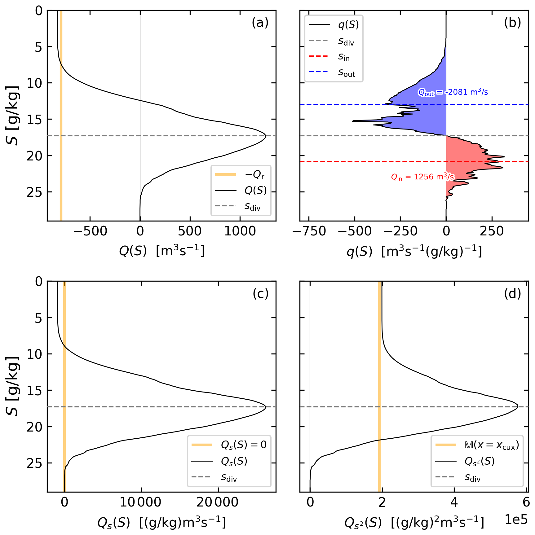
Figure 2TEF analysis using numerical model data from a cross-channel transect at along-channel position xcux at Cuxhaven near the mouth of the Elbe River estuary (see Fig. C1a), averaged for the full month of April 2024. (a) Volume transport Q(S) across the transect, with the freshwater discharge Qr and the dividing salinity sdiv for reference. (b) Volume transport per salinity class, q(S), as well as the bulk inflow and outflow salinities sin and sout, respectively. The shaded areas and written numbers correspond to the bulk volume inflow (Qin, red) and bulk volume outflow (Qout, blue). (c) Salinity transport Qs(S); (d) salinity-squared transport across the transect, with the integrated mixing within the estuarine volume bounded by the same transect, 𝕄(x=xcux), for reference.
Taking the S-derivative of Eq. (14) results in the volume, salinity and salinity-squared transport per salinity class (the Total Exchange Flow, TEF),
where the minus sign ensures that inflow at high salinities is positive to highlight the character of the exchange flow. The connection to the Knudsen relations Eqs. (18), (21) and (22) is given by separately integrating the positive and negative contributions (denoted by superscripts + and −) of the transport per salinity class,
and by deriving transport-weighted inflow and outflow salinities and squared salinities,
An exemplary TEF profile is found in Fig. 2b for the Elbe River estuary. Zero values for q(S) occur for extreme values of Q(S), in consistency with Eq. (15). For the two-layer exchange flow shown here, there is one unique maximum of Q(S), such that the salinity S at which this occurs is the dividing salinity sdiv between inflow and outflow (MacCready et al., 2018). Note that the dividing salinity sdiv can also be used to calculate the Knudsen parameters Qin, Qout, sin, and sout, providing a numerically more robust method compared to the direct computation via Eq. (16) (Lorenz et al., 2019). For multi-layer flows, multiple dividing salinities may occur (Lorenz et al., 2019; Burchard et al., 2025).
The TEF analysis framework has been applied for a variety of estuarine studies, such as for tidal estuaries (MacCready, 2011; Chen et al., 2012; Wang et al., 2017; Conroy et al., 2020; Lemagie et al., 2022; Reese et al., 2024), tidal bays (Gräwe et al., 2016; Rayson et al., 2017; Xiong et al., 2021; Lemagie et al., 2022), non-tidal estuaries (Lange et al., 2020; Burchard et al., 2025), inverse estuaries (Lorenz et al., 2020), fjords (Sutherland et al., 2011; Lemagie et al., 2022; MacCready and Geyer, 2024), and regional seas (Döös et al., 2004; Burchard et al., 2018a).
3.3 Knudsen theory
To assess how entire estuaries quantitively act as mixing machines, the local relations derived in Sect. 2.2 are now integrated over estuarine volumes. For this, the continuity equation Eq. (3) and the salinity equation Eq. (4) are first integrated over the estuarine volume V which is separated from the ocean by means of a fixed vertical transect:
(see Fig. 3a) with the inflow transport and representative salinity Qin≥0 and sin (the ocean water inflow), outflow transport and representative salinity Qout≤0 and sout (the brackish water outflow), as defined in Eqs. (16) and (17). Further quantities in Eq. (18) are the river run-off Qr≥0 (assuming zero river salinity for simplicity), the average salinity in the estuary , and the volume-integrated salinity . Details of the derivation of Eq. (18) are given in Burchard et al. (2019). The conservation laws Eq. (18) have already been formulated by Knudsen (1900) and have become the basis for analyses of exchange flow in many estuaries (see e.g., Ji et al., 2007; MacCready, 2011; Sutherland et al., 2011; Chen et al., 2012; Burchard et al., 2018a). The positioning of the transect that separates the estuarine volume from the ocean is arbitrary, but often the geographical location of the river mouth is chosen. In Eq. (18) freshwater transports across the surface (evaporation or precipitation), the bottom (submarine groundwater discharge) as well as horizontal diffusive salt transports across the transect are neglected. Relations including freshwater transport through the sea surface can be found in Lorenz et al. (2021). Under long-term averaged conditions, the volume and salt storage terms on the right-hand side of Eq. (18) would vanish. Under such circumstances, sout≤sin and must hold, as illustrated for the Elbe estuary in Fig. 4a, b, where balanced conditions with a nearly vanishing volume storage are given. Under such circumstances, inflow from the ocean occurs at higher salinities than outflow towards the ocean due to mixing with riverine water.

Figure 3Sketch showing the principles of volume and salt conservation as well as mixing in estuaries: (a) Estuarine volume (light blue shading) bounded by a fixed transect (bold red line), showing the classical Knudsen (1900) transports and salinities as well as the Knudsen mixing law Eq. (21) as derived by MacCready et al. (2018). (b) Estuarine volume (light blue shading) bounded by an isohaline of salinity S (bold blue line), showing the diahaline advective (Qdia) and diffusive transports (JS) as well as the mixing law Eq. (32) as derived by Burchard (2020). (c) Envelope of a discrete estuarine sub-volume (light blue shading) around the isohaline of salinity S (dashed blue line), bounded by the isohalines of salinities and (bold blue lines). The mixing per discrete salinity class is shown as well as the limit for S→0 which results in the universal law of estuarine mixing Eq. (33) for an infinitesimally thin salinity class. The bottom is marked by an orange line, the surface by a grey line and the fixed river transect by a red line. Advective volume transports are marked by blue arrows and the diffusive salt transport is marked by a yellow arrow.
The bulk mixing of an estuary is then obtained by averaging the integrated salinity variance budget Eq. (B2) in time:
with the estuarine bulk mixing
see the derivations by MacCready et al. (2018) and Burchard et al. (2019). In Eq. (19), the approximations and have been made for simplicity, where (s2)in and (s2)out are inflowing and outflowing salinity squares, respectively, as defined in Eq. (17). Assuming long-term averaging such that the temporal derivatives vanish and using Eq. (18), we finally obtain
(MacCready et al., 2018), relating the Knudsen parameters directly to estuarine mixing. While Knudsen (1900) had mentioned the role of mixing for the estuarine exchange flow qualitatively, Eq. (21) gave the first quantitative estimate of estuarine mixing as a function of the Knudsen parameters. An accurate bulk mixing estimate allowing and has been derived by Burchard et al. (2019):
For the special case of and , Eq. (21) is identical to Eq. (22). These equalities are only exact when the inflowing and outflowing salinities are constant in time and space during the averaging interval (Burchard et al., 2019). For estuaries with strongly fluctuating salinities at the mouth (such as for the short Merrimack estuary, see Chen et al., 2012) relation Eq. (22) has to be used instead of Eq. (21) to obtain an accurate estimate for the mixing.
Relation Eq. (21) is demonstrated in Fig. 4c for a numerical simulation of the Elbe estuary. It can be seen that the estimate is near-exact for almost the entire length of the estuary, proving its value for the study of bulk mixing in realistic estuaries, as also tested in studies by Broatch and MacCready (2022) and Reese et al. (2024).
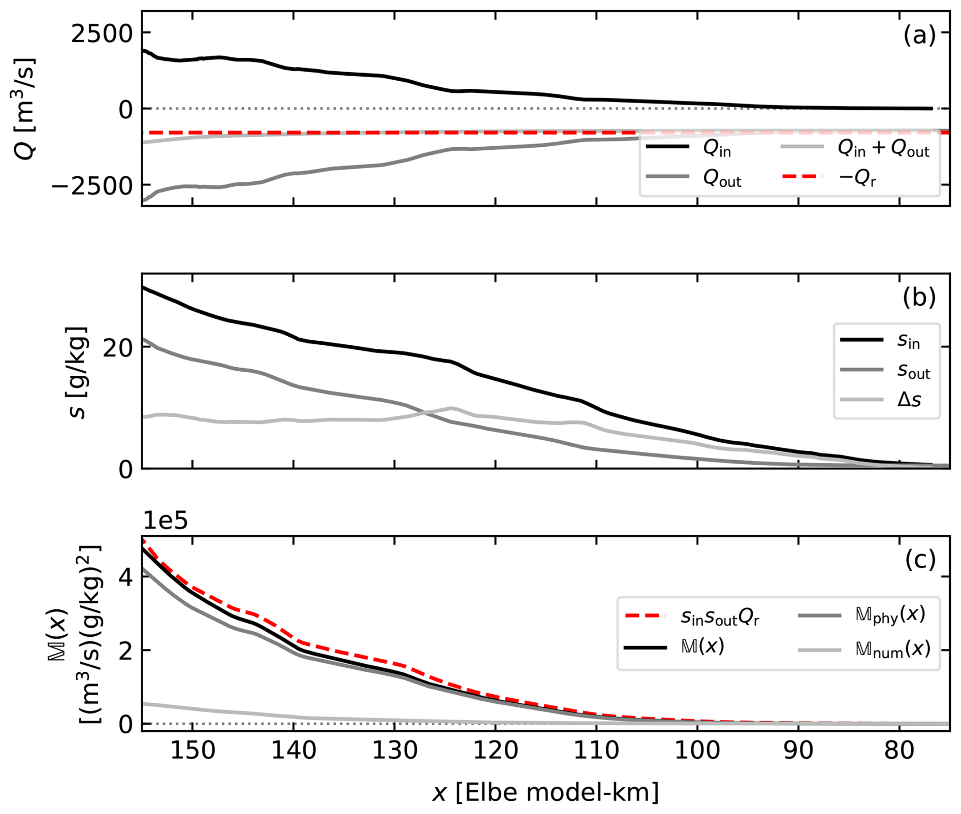
Figure 4Bulk parameters of the exchange flow through cross-channel transects at each along-channel position x from a numerical simulation of the Elbe River estuary, averaged for the month of April 2024. (a) Volume inflow and outflow Qin and Qout, respectively, compared to the freshwater discharge Qr. (b) Inflow and outflow salinities sin and sout, respectively, as well as their difference . (c) Integrated mixing 𝕄(x) within the estuarine volume bounded by a cross-channel transect at along-channel position x, split into the contributions of the physical mixing 𝕄phy due to the mixing parameterisation as well as the numerical mixing 𝕄num due to discretization errors. The directly computed mixing (solid lines) is compared to the mixing estimate Eq. (21).
The principle of salt mixing inside an estuary bounded by a fixed transect is sketched in Fig. 3a. The first relation of Eq. (21) shows that the mixing does also balance the exchange of squared salinity with the ocean, such that mixing can also be defined as the reduction of squared salinity integrated over the estuary (which often simplifies the calculations, see Burchard et al., 2019), as it is expressed locally in Eq. (B3). The second relation of Eq. (21) shows that estuarine mixing can be estimated simply by knowing inflowing and outflowing salinities and the river run-off (MacCready et al., 2018). The third relation of Eq. (21) demonstrates the relation between estuarine circulation (quantified as strength of Qin, see Broatch and MacCready, 2022; MacCready and Geyer, 2024) and mixing, a topic that is expanded on in Sect. 3.6.
Using the Knudsen relations Eq. (18), yet another useful reformulation of Eq. (21) has been derived by Qu et al. (2022) for estuaries in which the riverine inflow has non-zero salinity:
which is identical to Eq. (21) for a river salinity of sr=0. In Eq. (23), the right-hand side is split into two terms representing the mixing pathways from the inflows to the outflows, with the first one leading from the river inflow to the brackish water outflow and the second one leading from the seawater inflow to the brackish water outflow (with source-water salinities put first in the brackets).
The Knudsen mixing relation Eq. (21) has been extended by Lorenz et al. (2021) for the case of non-zero freshwater fluxes through the surface, i.e., precipitation and evaporation:
with the surface freshwater transport Qsurf (positive for net precipitation) and the representative surface salinity ssurf (square root of surface salinity variance transport divided by −Qsurf). Since for evaporation and for precipitation, both evaporation and precipitation are sources of mixing, in addition to the exchange flow. The example of the Persian Gulf as an inverse estuary with strong evaporation is briefly discussed in Sect. 4.1.3.
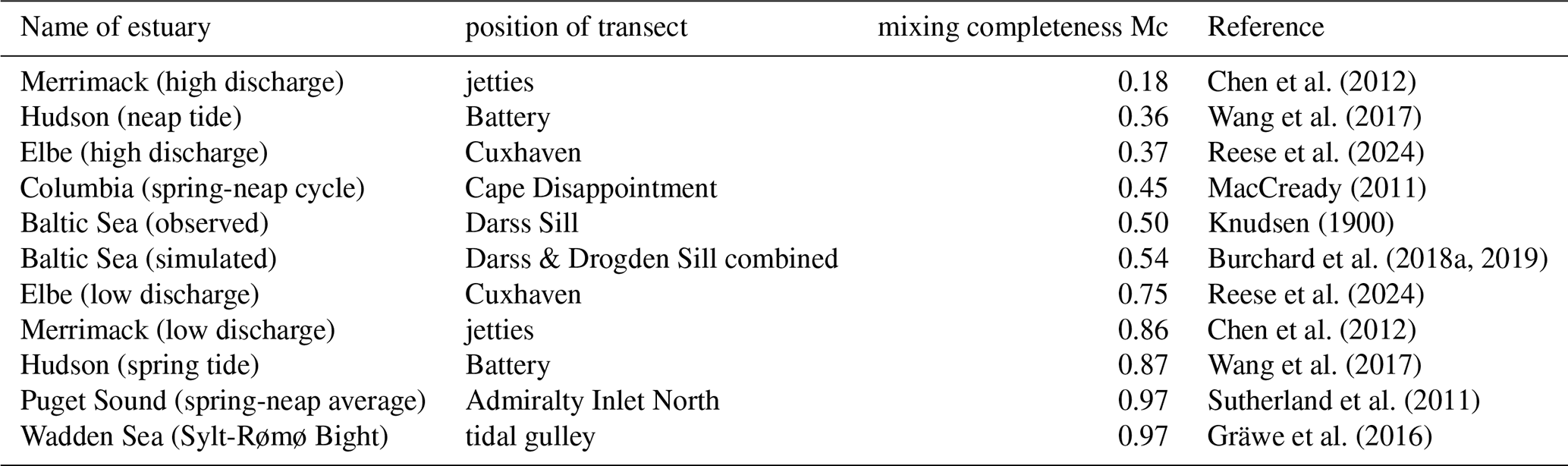
For the interpretation of the mixing relations it is instructive to consider the mixing completeness Mc (MacCready et al., 2018; Burchard et al., 2019) by non-dimensionalising Eq. (21) using Qr and sin:
where the river run-off Qr and inflowing salinity sin (sometimes equated to the ocean salinity) can be considered as the external forcing of the estuary. Mixing completeness in estuaries can cover the full range of theoretically possible values of . Table 1 gives a number of examples for estuarine systems with low, medium and high mixing completeness. It should be noted that the mixing completeness is always calculated with respect to a fixed transect and that for each estuarine system the mixing completeness varies strongly with discharge and tidal intensity (e.g., during the spring-neap cycle).
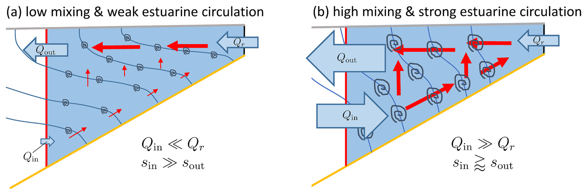
Figure 5Sketch showing estuarine conditions for low mixing causing weak estuarine circulation (a) and high mixing causing strong estuarine circulation (b). In both panels, Qr and sin are supposed to be identical. With prescribed low mixing 𝕄 in panel (a) and a high mixing 𝕄 in panel (b), the Knudsen relations Eqs. (18) and (21) quantify Qin, Qout and sout.
In the extreme case of no mixing, the riverine freshwater would flow out at the surface with no modification and no ocean water entering the system (sout=0 and Qin=0), such that the mixing completeness would be zero. In estuaries with low mixing, brackish water of only low salinity is produced, with sout≪sin and Qin≪Qr, such that the mixing completeness is , see sketch in Fig. 5a. This would theoretically be the case for deep fjords with low tidal energy (Inall and Gillibrand, 2010). Mostly, fjords do however have large water bodies and low discharge such that the freshwater is strongly diluted by tidal mixing as, for example, for the Puget Sound where the mixing completeness is as large as about 0.97 (see Sutherland et al., 2011, and Table 1). Low mixing values of about Mc=0.18 have been observed for the tidally intense Merrimack estuary during high discharge (see Chen et al., 2012). Under these conditions, the salt intrusion length shortens considerably such that high-salinity ocean water and low-salinity river water are in close contact at the mouth of this estuary discharging directly into the coastal ocean, leading to low mixing. Other low values of mixing completeness are also observed for the Hudson river estuary during neap tide (Mc=0.36, see Wang et al., 2017) and the Elbe River estuary at high discharge (Mc=0.37, see Reese et al., 2024). In both cases, the water is relatively strongly stratified in the region of the transect such that sout≪sin. The large variability that estuaries have due to changes in discharge and tidal intensity is demonstrated by the fact that the Elbe for low discharge, the Merrimack for low discharge, and the Hudson for spring show values of mixing completeness as high as Mc=0.75, Mc=0.86 and Mc=0.87, respectively. Almost complete mixing is obtained for the shallow Wadden Sea of the German Bight, as sketched in Fig. 5b. In the Sylt-Rømø-Bight, where the freshwater run-off is low and tidal mixing is high, Gräwe et al. (2016) calculated values of inflowing and outflowing salinity both >30 g kg−1 with only about 1 g kg−1 difference, such that the mixing compleness is about . These are values comparable to Puget Sound, see above. For the Baltic Sea, a non-tidal semi-enclosed sea in northern Europe, Knudsen (1900) estimated sin=17.4 g kg−1 and sout=8.7 g kg−1, such that the mixing completeness is Mc=0.5, a value that could be confirmed by a multi-decadal model simulation (Burchard et al., 2018a, 2019).
Chen et al. (2012)Wang et al. (2017)Reese et al. (2024)MacCready (2011)Knudsen (1900)Burchard et al. (2018a, 2019)Reese et al. (2024)Chen et al. (2012)Wang et al. (2017)Sutherland et al. (2011)Gräwe et al. (2016)Table 1List of estuarine systems with typical values of mixing completeness Mc for different tidal and runoff conditions. Note that estuaries with strong temporal variation (e.g., the Hudson River estuary during the spring-neap cycle) are not in balance, such that Eq. (25) is only a rough approximation.
3.4 Water Mass Transformation and diahaline mixing
Often, it is instructive to consider dynamics of estuaries in an isohaline framework, i.e., to evaluate transports, mixing and other properties relative to moving surfaces of constant salinity (isohalines) instead of the Eulerian framework with fixed spatial coordinates. With this, a quasi-Lagrangean perspective is added to the analysis with reference to the moving flow. In the isohaline analysis, geographical features such as a fixed transect at the mouth of the estuary do not play a central role. Since isohalines can move inside and outside the estuarine water body and extend over large areas covering parts of the estuary and the river plume, the isohaline analysis treats estuary and river plume as a dynamic continuum. This isohaline view of estuarine dynamics was first proposed by Walin (1977), with specific reference to the Baltic Sea with its isohalines extending over up to 1000 km from the Central Baltic Sea to its Western reaches (Henell et al., 2023). Later, the isohaline concept was applied to tidal estuaries (MacCready and Geyer, 2001; MacCready et al., 2002; Wang et al., 2017) and river plumes (Hetland, 2005; Muche et al., 2026). Here, we first introduce a local diahaline analysis, before we discuss the bulk analysis of estuarine dynamics across isohaline surfaces in Sect. 3.5.
Local mixing can move isohaline surfaces vertically such that a diahaline mass transport occurs relative to the moving isohaline surface. When normalised to isohaline unit surface and unit mass, this results in a so-called entrainment velocity. Starting for explanation with the one-dimensional salinity budget equation Eq. (D3), a coordinate transformation from geopotential z to salinity coordinates s (assuming a stable salinity stratification with ), after time averaging in salinity coordinates, 〈⋅〉S, a formulation for the vertical entrainment velocity udia,z(S) (vertical velocity relative to the vertically moving isohaline) is obtained:
(Wang et al., 2017; Klingbeil and Henell, 2023), where jdia,z(S) is the time-averaged upward salinity flux through the moving isohaline. The vertical velocity of the isohaline S due to both advection and turbulent diffusion is given by (with z being the vertical position of the isohaline). Details of the derivation of Eq. (26) are given in Eqs. (D1)–(D3). The meaning of Eq. (26) is sketched in Fig. 6a: there is a maximum of vertical turbulent salinity flux jdia,z in the entrainment layer that caps the turbulent bottom boundary layer. This maximum results from a large vertical salinity gradient at a still high level of turbulence originating from the boundary layer, expressed as eddy diffusivity Kv. Below this maximum, vertical salinity flux is divergent, thus lowering the local salinity which in time-average leads to an upward entrainment velocity udia,z. Above the entrainment layer, the opposite happens, resulting in a downward salinity flux. A similar process has been described and sketched by Ferrari et al. (2016), using density fluxes near the bottom of the ocean. The exchange flow in the bottom boundary layer itself with upwelling near the bottom and downwelling above has already been described by Garrett (1991). It should be noted that the total diahaline salt flux consists of two contributions, with one advective contribution and one diffusive contribution:
with the consequence that volume flux and salt flux are not proportional to each other and that the distribution of the diffusive salt flux in salinity coordinates entirely determines the total diahaline salt flux.
To relate jdia,z to mixing χs, Li et al. (2022) defined the local mixing per salinity class which for a vertical water column with a monotone salinity profile reads as
which can be seen as a thickness-weighted time-average of the local mixing χs, see also Klingbeil et al. (2019), Burchard et al. (2021) and Li et al. (2022). Combining Eqs. (26) and (28) results in a key relation between entrainment velocity and mixing,
which could be called the diahaline mixing-entrainment relation. Note that here upward velocities udia,z and fluxes jdia,z are denoted as positive quantities. Details of the derivation of Eq. (29) for non-monotone salinity distributions in three dimensions can be found in Klingbeil and Henell (2023). The principle of Eq. (29) is sketched in Fig. 6b: as given by Eq. (28), m has local maxima in the same locations as jdia,z, i.e., in the entrainment layers. For mixing per salinity class increasing with height, (for stable salinity stratification), a positive entrainment velocity is expected. For mixing decreasing with height, the opposite occurs. This leads to a typical pattern of diahaline exchange flow in estuaries with positive (upward, towards lower salinities into the estuary) entrainment through an isohaline near the bottom, and a negative (downward, towards higher salinities out of the estuary) entrainment through the same isohaline near the surface further seawards. For realistic estuaries this has been shown for the Hudson River estuary (Wang et al., 2017), the Pearl River estuary (Li et al., 2022, 2024), the Elbe River estuary (Reese et al., 2024), the Changjiang River estuary (Chang et al., 2024) and the Baltic Sea (Henell et al., 2023). In particular, Henell et al. (2023) and Reese et al. (2024) calculated both sides of Eq. (29) independently to demonstrate their equality (aside from small numerical differences) in real-world estuarine systems. The advantage of Eq. (29) over Eq. (26) is given by the fact that χs and thus m can be split into physical and numerical contributions (see Sect. 5.2.2), such that numerically generated spurious entrainment can be calculated, as shown by Henell et al. (2023) for the Baltic Sea.
The relationship between diahaline mixing m and entrainment velocity udia,z across the isohaline of 11 g kg−1 is shown in Fig. 7 for the Elbe River estuary in northern Germany. It is clearly visible that as stated in Eq. (29), entrainment requires mixing since hotspots of the two quantities align well. In the up-estuary reach of the isohaline surface, where it is close to the bottom, upwelling (red) dominates, whereas at the down-estuary near-surface reaches of the isohaline downwelling (blue) dominates.
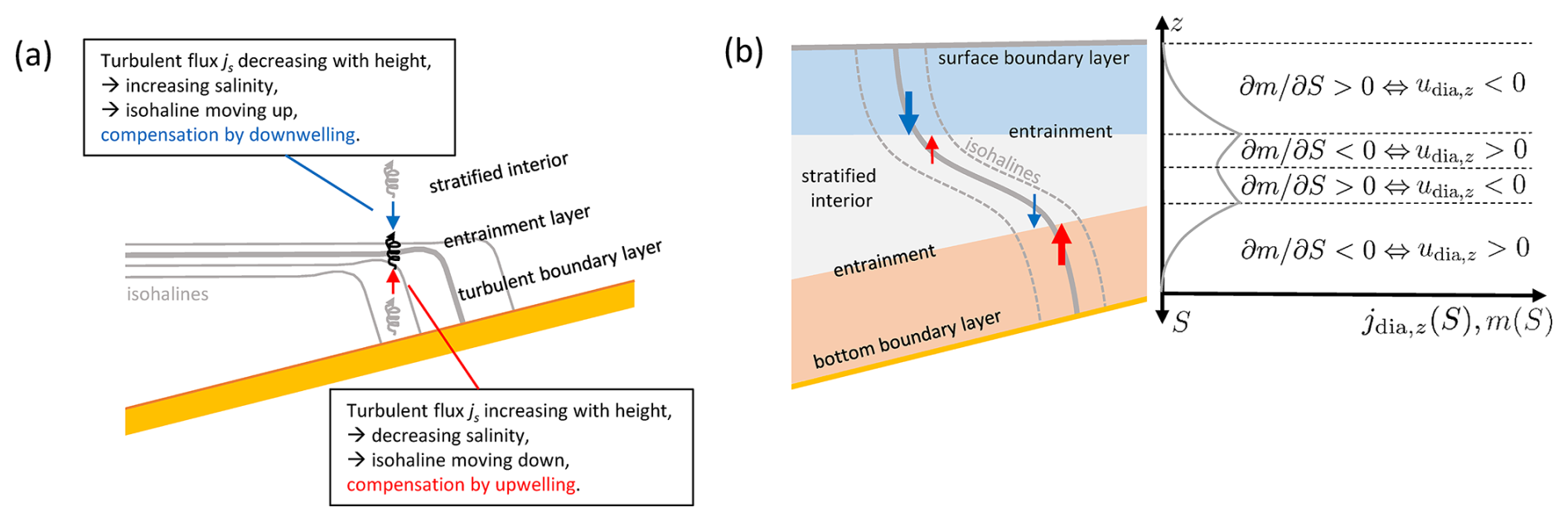
Figure 6Sketch demonstrating the mechanism and distribution of diahaline exchange flow in estuaries. (a) Generation of diahaline exchange flow by means of a divergent vertical turbulent salinity flux jdia,z, according to Eq. (26), shown for the bottom boundary layer of an estuary. High values of jdia,z are marked by a black whirl, and low values are marked by grey whirls. The entrainment velocity is marked as red (upwards, ) and blue (downwards, ) arrows. (b) Situation of time-averaged diahaline exchange in an estuary. The bottom boundary layer and the surface boundary layer are marked by colour, both being separated from a more stratified interior via entrainment layers. Three exemplary isohalines are drawn. The entrainment velocity is again marked as red and blue arrows, where the size of the arrows corresponds to its relative magnitude. On the right side of the sketch a typical profile of the local mixing per salinity class m(S) is shown, along with consistent signs of the entrainment velocity udia,z, according to Eq. (29).
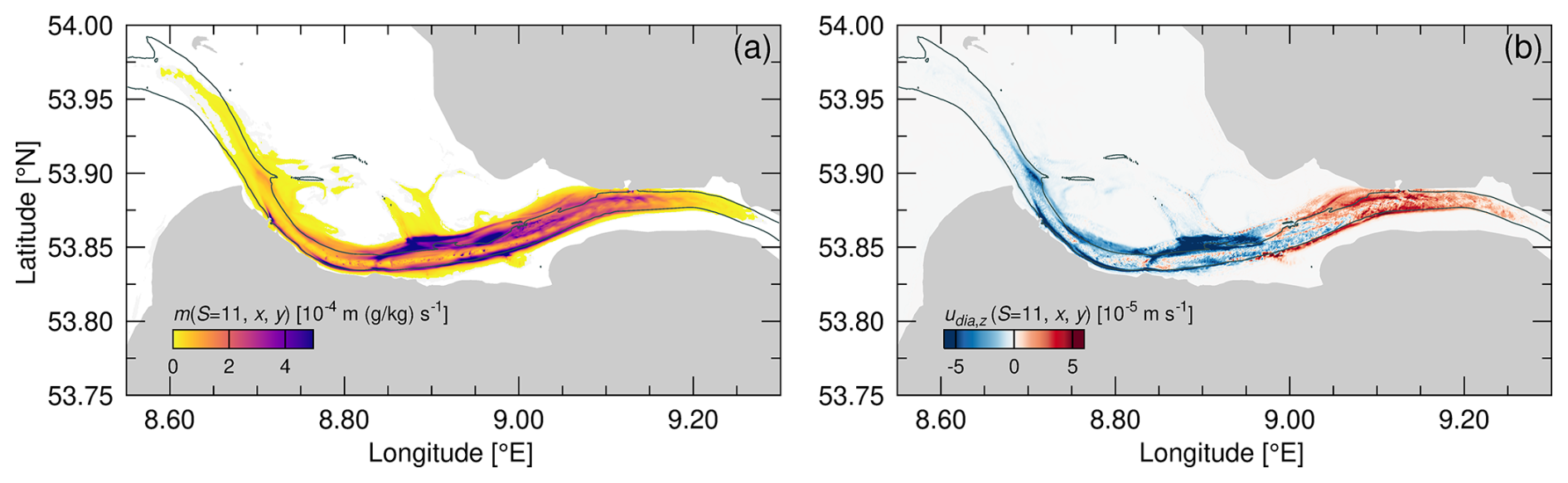
Figure 7Diahaline mixing m (a) and diahaline entrainment velocity udia,z (b) across the isohaline surface of 11 g kg−1, averaged over two spring-neap cycles during April 2024 in the lower Elbe River estuary in Germany. The line in both panels shows the 10 m isobath.
3.5 Estuarine mixing in isohaline volumes
Local diahaline mixing as introduced in Sect. 3.4 can be expanded to estuarine volumes (Walin, 1977). The local relation Eq. (27) for the total diahaline salt flux fdia,z(S) can be integrated over the entire isohaline surface to result in
where Fdia is the total salt transport, Qdia<0 is the diahaline volume transport, and Jdia>0 is the diffusive salt transport across the isohaline surface (see Fig. 8a by Walin, 1977). If instead of a fixed transect T a moving isohaline of salinity S is considered as the seaward boundary of the estuary (see Fig. 3b), the volume and salt budget is of this form:
with the isohaline volume V(S), the average salinity inside this volume , the net advective inflow through the isohaline, , and the the net advective outflow through the isohaline, . Transformations of Eq. (31) show that long-term averaged mixing inside the estuarine volume bounded by an isohaline S is
which can be seen as a special case of 𝕄≈sinsoutQr from Eq. (21) with (Burchard, 2020). The relation Eq. (32) is exact for long-term averaging and zero freshwater transports through the surface and bottom of the estuary. A mixing relation for non-zero river salinity is shown in Eq. (F27).
With 𝕄(S) being a continuous function of S and assuming that Qr is independent of S, we can take the derivative of M(S) with respect to S:
where 𝕞(S) is the salt mixing per salinity class. It should be noted that 𝕞(S) can also be obtained by integrating the local mixing per salinity class m(S) from Eq. (29) over the projection of the isohaline surface to the horizontal (Li et al., 2022). A discrete version of Eq. (33) is sketched in Fig. 3c in order to explain the infinitesimal property of the mixing per salinity class. The linear dependence of 𝕞(S) on salinity S has been formulated and derived as the universal law of estuarine mixing (Burchard, 2020).
The relation Eq. (33) can be explained by first stating that the volume transport across the isohaline must for long-term averaged conditions equal the river runoff Qr. Furthermore, the advective salt transport across the isohaline, , must equal the diahaline diffusive salt transport, such that Jdia(S)=SQr, see the second equation in Eq. (31). With
which can be derived by integration of Eq. (28) over the horizontal projection of the isohaline surface, relation Eq. (33) is obtained (Burchard et al., 2021). A relation equivalent to the combination of Eqs. (33) and (34) had been derived by Hetland (2005), based on earlier work of Garvine (1999), to quantify the turbulent salt transport into river plumes due to entrainment, see the steady-state version of his Eq. (4).
To accurately reproduce the universal law by means of models of realistic estuaries such as the Pearl River estuary (Li et al., 2022), the Changjiang River estuary (Chang et al., 2024) and the Elbe River estuary (Reese et al., 2024), averaging over one spring-neap cycle is typically sufficient. In a numerical model, the mixing which a salinity field experiences is the sum of the parameterised physical mixing 𝕞phy(S) and spurious numerical mixing 𝕞num(S) due to the discretisation of the advection operator, see Sect. 5.2.2 for details. Both, relations Eqs. (32) and (33), are tested for the Elbe estuary in Fig. 8. There, it can be seen that the directly computed total mixing quantities 𝕄(S) and 𝕞(S), each consisting of the sum of numerical and physical mixing, closely follow their respective relation up to the point where the isohaline surfaces partly leave the model domain through the open boundary (grey-shaded areas in the Figure). Here, we first find an underestimation of the predicted mixing by relations Eqs. (32) and (33) which can likely be related to left-over stratification in the German Bight from earlier high-discharge periods entering the model domain via the open boundary and then being mixed away. For very high salinity classes, the mixing in the model is much weaker than the predicted mixing since substantial parts of the isohaline surfaces are outside of the model domain such that most of the potential mixing is not covered by the model. While the Knudsen mixing law Eq. (21) is only valid when salinity fluctuations at the open boundary are limited, the universal law of estuarine mixing, Eqs. (32) and (33), is exact for all estuaries (without relevant freshwater fluxes across the sea surface).
One interesting consequence of the universal law of estuarine mixing can be seen by reformulating Eq. (33) as
where 𝕧(S) is the volume per salinity class and is the salinity mixing averaged over the salinity class S. Since for long-term averages is fixed, Eq. (35) means that at low mixing rates the volumes per salinity class should be large, with the consequence that at low mixing rates, isohaline spacing should be wide. When comparing for example the salinity fields for the Hudson River estuary for neap tide and for spring tide (Warner et al., 2005a), the isohaline spacing at springs is wider than at neaps. Assuming that storage terms do not play an essential role for these situations, the conclusion could be drawn that average mixing is smaller at springs than at neaps. This is consistent with the findings of Warner et al. (2020) who find that maximum mixing occurs during late neap tides, see also Sect. 4.1.2. This is also in line with the study of Garvine (1999) who showed that increased (background) diffusivity would reduce the area of a river plume (see also the river plume study by Li et al., 2024, who showed that additional mixing due to islands in the plume region can reduce the plume area and volume).

Figure 8Salt mixing from a realistic numerical simulation of the Elbe River estuary, averaged for the full month of April 2024. (a) Integrated mixing 𝕄(S) within an estuarine volume bounded by an isohaline surface of salinity S as computed directly from numerical model data (solid black line) as well as from the freshwater discharge Qr using equation Eq. (32) (dashed line). (b) Mixing per salinity class 𝕞(S) as computed directly from numerical model data (solid black line) as well as from the universal law of estuarine mixing, Eq. (33) (dashed line). In each panel, the respective contributions of the physical mixing 𝕄phy and 𝕞phy due to the mixing parameterisation as well as the numerical mixing 𝕄num and 𝕞num due to discretisation errors to the total diagnosed mixing are shown as solid grey lines.
3.6 Relating estuarine circulation to mixing
In his famous abyssal recipes Munk (1966) fitted a vertical one-dimensional advection-diffusion equation to hydrographic observations in the central Pacific Ocean and concluded that turbulent mixing with an effective vertical diffusivity of m2 s−1 would be needed to explain the global overturning circulation. In later studies, the decomposition of the underlying mixing processes into wind and tidal mixing and their regional distribution had been further specified (see e.g., Munk and Wunsch, 1998; Kuhlbrodt et al., 2007; Nikurashin and Ferrari, 2011; Cessi, 2019). On the much smaller scales of estuaries, the same must be postulated: estuarine circulation requires mixing and vice versa. Here, we discuss different concepts of this duality.
Let us first summarise what we have discussed about this issue until now. In his fundamental paper, Knudsen (1900) already stated that estuarine circulation is associated with mixing (Sect. 1). The general process is that salty ocean water entering the estuary is first mixed with fresh river water inside the estuary and then ejected as brackish water towards the ocean, making estuaries mixing machines (MacCready and Banas, 2011; Wang et al., 2017). When there is no mixing inside the estuary, then no further salty water can enter the estuary in the long term (Sect. 3.3). In that sense, the volume transport of salty water flowing into the estuary, Qin, is a good measure for the estuarine circulation (Broatch and MacCready, 2022; MacCready and Geyer, 2024). A first quantitative estimate for the tight relationship between estuarine circulation and mixing has been established in the third relation of Eq. (21) by MacCready et al. (2018), showing a proportionality between the bulk mixing 𝕄 and Qin, with (sin−sout)sin as factor of proportionality.
The streamfunction Q(S) of the estuarine circulation as defined in Eq. (14) is the time-averaged volume transport into the estuary across a fixed transect for all salinities above S and therefore contains the information about the Total Exchange Flow, see Sect. 3.2 for details. It can be directly linked to mixing, as derived already by Walin (1977) to quantify the overturning circulation of the Baltic Sea:
where the subscript est means that diahaline transport Qdia, diahaline salt flux Jdia and diahaline mixing per salinity class 𝕞 are only considered for the part of the isohaline that is located on the estuarine side of the transect, see Fig. 9. The first equality in Eq. (36) is demonstrated in Fig. 9a: under long-term averaged conditions the volume transport Q(S) into the subvolume bounded by the transect T, the isohaline S and the bottom must be equal to the volume transport across the isohaline S, Qdia,est(S). The second equality in Eq. (36) results from the integration of the entrainment relation Eq. (26) over the projection of the isohaline part situated upstream of the transect T. The third relation of Eq. (36) which had not been proposed by Walin (1977) is simply the S-derivative of Eq. (34) restricted to the upstream part of the estuary. Walin (1977) stated about this relation (his Eq. 7): Equation (36) represents in the most simple way how the deep water supply is related to the overall vertical (i.e. cross-isohaline) mixing properties in the basin. What Walin (1977) specifically calls the deep water supply to the Central Baltic Sea is more generally the up-estuarine part of the estuarine circulation. Note that independently of Walin (1977), Wang et al. (2017) used the first two equalities of Eq. (36) to calculate exchange flow accumulated between two estuarine segments.
When choosing the dividing salinity S=sdiv for relation Eq. (36) with Q(sdiv)=Qin (see Sect. 3.2), then the quantification of the estuarine circulation is directly linked to mixing:
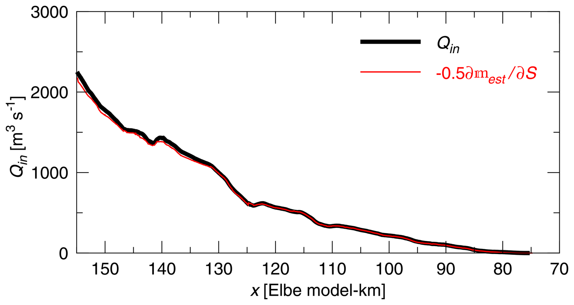
see details in Burchard et al. (2025) and Fig. 9b. The significance of Eq. (37) is that it is a direct quantification of the estuarine circulation (defined as Qin) by means of the (S-gradient of the) diahaline mixing. This relation is directly applicable to simple estuaries with a typical two-layer exchange flow, but has also been extended to multi-layer exchange flow (Burchard et al., 2025). For the Elbe River estuary, relation Eq. (37) is demonstrated in Fig. 10.
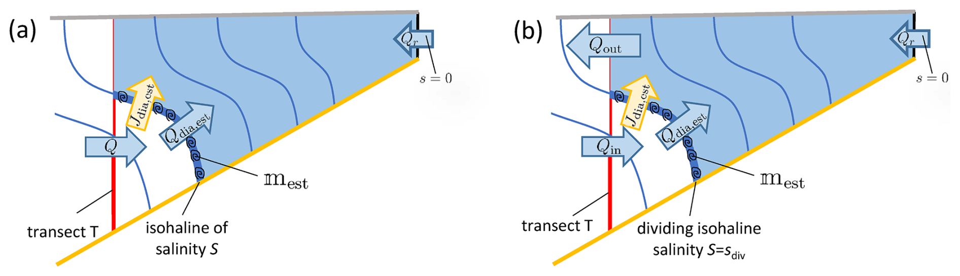
Figure 9Sketch showing the relation between estuarine circulation and diahaline mixing. (a) Demonstration of the relation Eq. (36) by Walin (1977). (b) Demonstration of the relation Eq. (37) by Burchard et al. (2025) using the dividing salinity isohaline to quantify the exchange flow by means of Qin.
3.7 Mixing of other constituents than salt
This review focuses on mixing of salt. The reason is that salinity is the defining constituent of estuaries, continuously ranging from minimum values near zero in the river water towards ocean salinity values near the mouth of the estuary or in the river plume. Therefore, salinity can be used as a coordinate in estuaries (Walin, 1977) substituting spatial coordinates. Also, salinity is conservative with basically no inner sinks and sources, and also bottom and surface fluxes of salt are negligible. However, many other constituents are mixing in estuaries, such as heat, oxygen, nutrients, and pollutants. Based on the work of Walin (1977, salinity coordinates) and Walin (1982, temperature coordinates), for larger ocean scales, theoretical Water Mass Transformation (WMT) frameworks have been developed to analyse mixing of constituents other than salt (Hieronymus et al., 2014; Groeskamp et al., 2019). To evaluate non-conservative behaviour of estuarine tracers due to sources or sinks, such tracers are often represented as function of salinity (Boyle et al., 1974). By doing so, non-conservative tracer mixing is identified by a non-linear relation between tracer concentration and salinity. However, as shown by Loder and Reichard (1981), such non-linear behaviour could also be caused by tracer variability in the freshwater source of the estuary. There is a large body of literature about effects of estuarine mixing of tracers other than salt on ecosystem dynamics. For example, Geyer (1993) proposes differential vertical mixing of suspended particulate matter (SPM) as a mechanism of creating Estuarine Turbidity Maxima. Tidal covariance between longitudinal velocity and concentration of SPM due to vertical SPM mixing can lead to up-estuary SPM transport (Scully and Friedrichs, 2007). In a similar way, Scully et al. (2022) explain the generation of local maxima of carbon dioxide partial pressure in estuaries, the so-called Estuarine Gas Exchange Maxima. Nitrogen-to-phosphate ratios in estuaries has been shown to critically depend on tidal mixing (Lui and Chen, 2011). These are just a few examples which show the essential role of mixing of tracers other than salt in estuaries. However, a general theory for such tracer mixing has not yet been proposed.
In the previous chapters we have presented various local and bulk theories of mixing and showed examples for the Elbe River estuary. These theories and examples prove that mixing, defined as integrated or local salinity variance decay due to turbulent processes, is an ubiquitous element in estuaries. Moreover, mixing defines what an estuary, consisting of a mixture of ocean and river water, is. While we know from the bulk mixing rules for estuaries, e.g., the Knudsen mixing law Eq. (21) or the universal law of estuarine mixing Eq. (33), how strong the overall mixing is in an estuary, we need to understand where the mixing occurs in time and space and which processes drive it. The intensity of mixing in an estuary is dictated by Eq. (10), , indicating that mixing depends linearly on the intensity of turbulence, as expressed by the vertical diffusivity, and quadratically on the strength of the vertical salinity gradient. Typically in estuaries, the stronger the turbulence, the weaker the vertical salinity gradient, so it is not obvious a priori where and when mixing will be maximal in an estuary. In this section, the mixing in the Elbe estuary (and in one case that of the James River estuary) is used to provide an example of the various factors influencing the temporal and spatial variation of mixing in a partially mixed estuary.
4.1 Temporal variability
In estuaries, various time scales are relevant, including semi-diurnal tidal time scales and the fortnightly spring-neap cycle as well as times scales of weather and river-run-off (days to months). In the subsequent sections, the most relevant processes on these time scales are discussed.
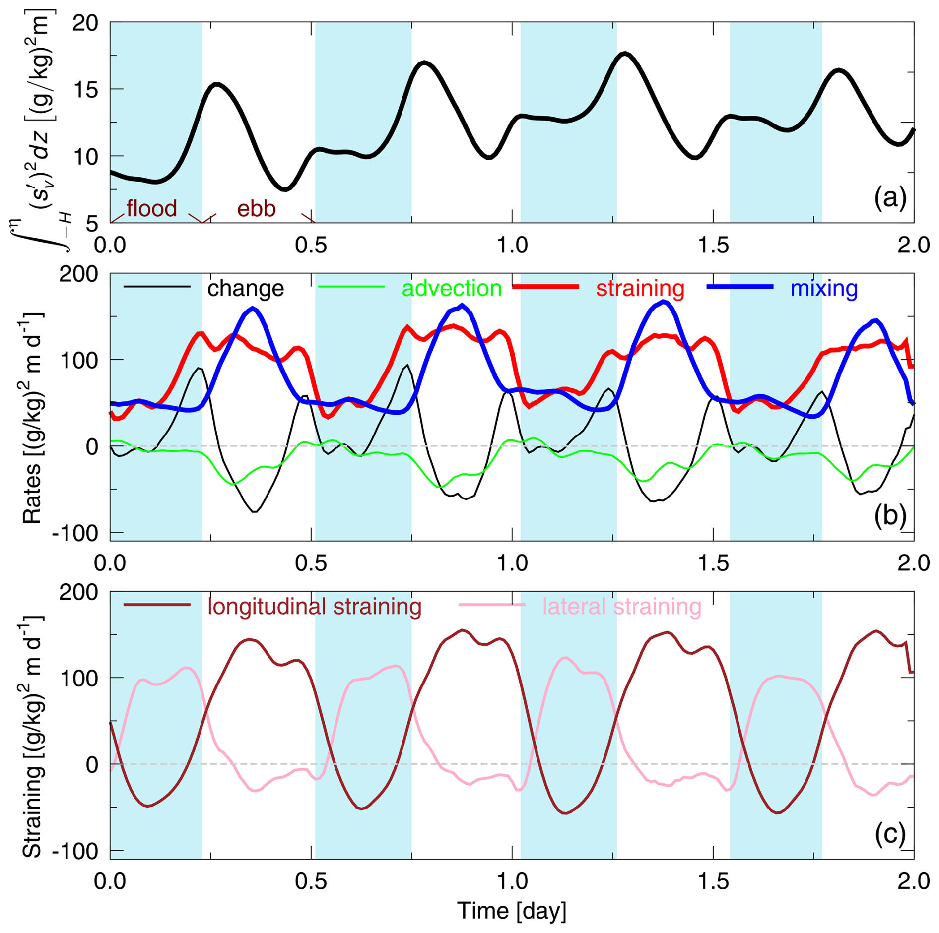
Figure 11 Dynamics of vertical salinity variance, spatially averaged over the Elbe River estuary domain between river kilometres 85 and 160, during four tidal cycles. (a) Vertical salinity variance; (b) Terms in the variance budget Eq. (12); (c) Straining term split into longitudinal and lateral components.
4.1.1 Tidal variability
An analysis of the tidal cycle of the vertical salinity variance in the Elbe River estuary using Eq. (12) averaged over most of the estuary demonstrates the sequence of processes driving mixing (Fig. 11).
Panel (a) of Fig. 11 indicates that the vertical variance shows considerable variation through the tidal cycle, sharply rising at the end of flood, then decreasing to a minimum near the end of ebb. Panel (b) of Fig. 11 shows the individual terms in the vertical variance balance Eq. (12). Lateral straining is strongest during the flood tide (Fig. 11c). It accounts for most of the increase in stratification (as expressed by total vertical variance) toward the end of the flood tide, but it has little correspondence with mixing. This contribution of lateral straining has been observed in other estuaries (Purkiani et al., 2015; Geyer et al., 2017), with the important consequence that it produces a maximum in stratification at the beginning of the ebb tide. The longitudinal strain is actually negative during the flood (i.e., weakening stratification), but it is strongly positive during the ebb. This is the well-known signal of tidal straining, first described by Simpson et al. (1990). Particularly notable are the mid-ebb peaks in mixing, which are almost exactly in phase with the peak in longitudinal straining. This correspondence between longitudinal straining during the ebb and estuarine mixing has been found in other partially mixed estuaries including the Hudson River estuary (Wang and Geyer, 2018; Warner et al., 2020) and also the more strongly stratified Changjiang River estuary (Li et al., 2018) and Connecticut River estuary (Holleman et al., 2016).
Why is longitudinal straining so effective at increasing estuarine mixing? Going back to Eq. (10), we see that the intensity of mixing depends more sensitively on stratification than on the turbulence itself, although both are necessary to generate mixing. The positive strain that occurs during the ebb provides a continual source of stratification, which roughly balances the destruction of stratification by mixing during a significant fraction of the ebb tide (the times when the longitudinal strain and mixing have equal magnitude in Fig. 11). Paradoxically, the increased stratification during the ebb actually has an inhibitory influence on turbulence, but this inhibition of turbulence causes an enhancement of the vertical shear during the ebb. Figure 12 shows representative vertical profiles of velocity u, salinity s, eddy diffusivity Kv and mixing χs during flood and ebb in the Elbe estuary. The strong mixing that occurs during the ebb is found in the stratified boundary layer, in which the eddy diffusivity is actually much weaker than its value during the flood tide. The key to the mixing is the persistence of stratification, which is maintained by the strong shear that strains the along-estuary density gradient. Even though turbulence is weakened by stratification, it is not completely suppressed, due to the turbulence production originating from the bottom stress. During the flood tide, the boundary layer produces virtually no mixing, due to the absence of stratification. The only significant mixing occurs in the pycnocline when the well-mixed highly turbulent bottom boundary layer is entraining into the stratified layer above, where the turbulence is much weaker than the boundary layer but the stratification is strong. This shows that maximum mixing does not occur at the maxima of eddy diffusivity or salinity stratification, but at locations where both overlap (see also Warner et al., 2020, who report similar results for the Hudson River estuary).
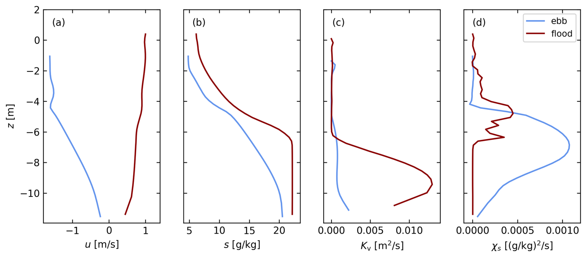
Figure 12Simulated vertical profiles of (a) the along-channel current velocity u, (b) salinity s, (c) vertical eddy viscosity Kv, and (d) local salt mixing χs from a near-shoal location within the inner Elbe River estuary at along-channel position x=127 km for ebb (blue) and flood (red), respectively, during a neap tidal cycle. The data was averaged over five neighbouring grid cells, corresponding to an along-channel distance of 360 m. Temporally, the data was averaged for one hour around peak ebb and peak flood, respectively.
4.1.2 Spring-neap cycle
The spring-neap cycle of tidal amplitude variation results in a large variation in the intensity of mixing, as shown in a timeseries based on the numerical model of the Elbe estuary. As often observed in partially mixed estuaries, the stratification (as represented by vertical variance, Fig. 13b) shows a large variation over the spring-neap cycle, with a sharp peak in stratification each neap tide. Again we have the paradoxical result that the peak mixing occurs during neap tides (Fig. 13c), when turbulent intensity is the weakest. Returning to Eq. (10), the mixing depends on the square of the vertical salinity gradient but only linearly on the eddy diffusivity. According to estuarine theory, stratification varies roughly as (MacCready and Geyer, 2010), so the increased stratification is a much more important contributor to mixing than Kv through the spring neap cycle.
The timeseries of longitudinal strain through the spring-neap cycle (Fig. 13c) shows that it has similar spring-neap variation as mixing. The strain is a key ingredient for mixing – without it the stratification would vanish and there would be nothing to mix. The strain increases during neap tides due to the increased stratification, which augments the horizontal strain term in Eq. (12) directly by the increase in , and indirectly by the stratification-induced reduction in eddy viscosity, which increases (MacCready and Geyer, 2010).
Other estuaries show a different phase relationship between mixing and the spring-neap cycle. For example, in the Hudson River estuary the peak mixing occurs between neaps and springs (Wang and Geyer, 2018), and in the Changjiang River estuary outflow the peak mixing occurs during spring tides (Li et al., 2018). These variations in the timing of mixing are related to the relative strength of tidal forcing to the stratifying tendency of the estuarine circulation. This balance is represented by the Simpson number as defined in Eq. (13). In the Elbe River estuary, Si remains low for most of the spring-neap cycle, with strong stratification only occurring around the time of neap tides. The Hudson River estuary has higher values of Si, and the Changjiang higher still, leading to persistent stratification through the spring-neap cycle (Li et al., 2018). A closer look into the dynamics of the Changjiang River estuary reveals that most of the mixing occurs outside the estuary in the extensive river plume, due to the high river discharge (Li et al., 2018; Chang et al., 2024). In the sense of the universal law of estuarine mixing (32), this can also be formulated as follows: Since the estuary is relatively fresh during high-flow conditions, mixing inside the estuary is small. Therefore strong mixing must occur outside the estuary, i.e. in the river plume, to amount to 𝕄(S)=S2Qr, where here S is a salinity separating the estuary – river plume continuum from the adjacent coastal ocean. In this high Si regime, the strength of the turbulence becomes the limiting factor controlling mixing, leading to the peak mixing during spring tides.
Although these studies did not investigate the processes of mixing in detail, neap tidal turbulence might not be sufficiently strong to entrain the turbulent bottom boundary layer into the region of the surface-attached buoyant plume and cause mixing. Therefore, substantial near-surface salinity stratification remains until spring tides reduce it by mixing. In general it could be hypothesised that in tidally energetic estuaries vertical salinity variance is mixed away immediately once it is generated by straining during neap tides, as in the Elbe, Hudson and Pearl River estuaries. In stratified estuaries, this mixing process is delayed until spring-tide turbulence can efficiently mix, as in the Changjiang River estuary.
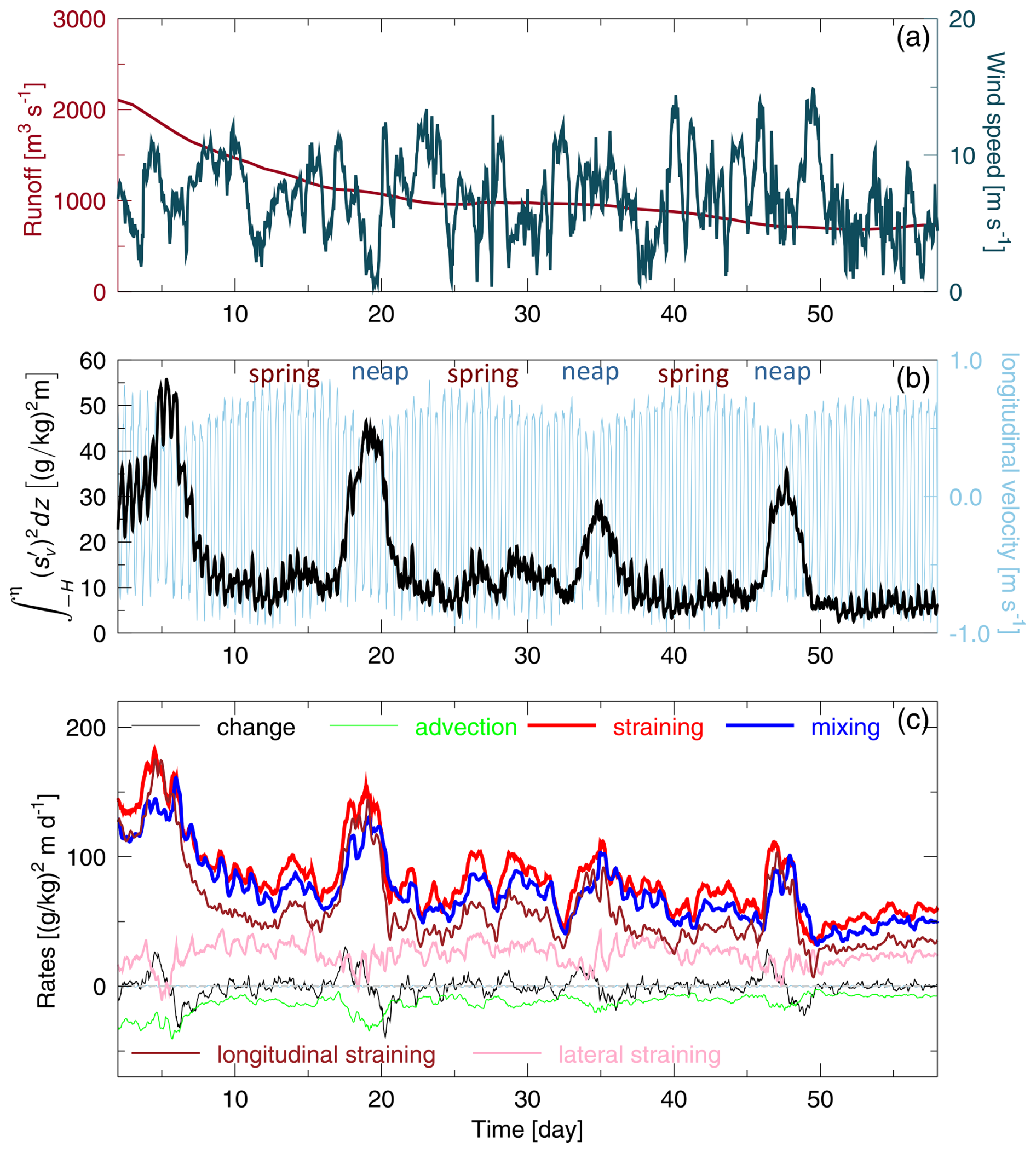
Figure 13 Dynamics of vertical salinity variance, spatially averaged over the Elbe River estuary domain between river kilometres 85 and 160, during four selected spring-neap cycles, as well as forcing conditions. (a) Runoff and wind speed; (b) vertical salinity variance and longitudinal tidal velocity amplitude; (c) terms of the vertical salinity budget according to Eq. (12).
4.1.3 Variation with variance input and direct meteorological forcing
In estuaries, there are four boundaries through which salinity variance can be introduced: the river boundary (river discharge), the seaward boundary (salinity fluctuations at the mouth), the sea surface (evaporation and precipitation) and the bottom (groundwater discharge, which we do not further consider here).
The bulk mixing laws for estuaries show clearly that under balanced conditions, mixing should be proportional to the river runoff Qr. This is obvious from the Knudsen mixing law in an estuarine volume bounded by a fixed transect, 𝕄=sinsoutQr, (see Eq. (21) as proposed by MacCready et al., 2018) and for the universal law of estuarine mixing inside a volume bounded by an isohaline surface of salinity S, 𝕄(S)=S2Qr, (see Eq. (32) as proposed by Burchard, 2020). Since these two theories are based on long-term averaging, time lags between changes in runoff and changes in mixing are expected due to the storage of volume, salt and salinity variance (Broatch and MacCready, 2022). The dependence of mixing on runoff has most impressively been shown in the study by Broatch and MacCready (2022) for the Puget Sound: When the runoff during summer becomes four times larger than the spring runoff, mixing increases roughly by the same factor, showing a much stronger signal than the spring-neap cycle. This is specifically supported by the universal law Eq. (32): Since the salinity at the mouth of the large Puget Sound might not change much, the volume-integrated mixing should be largely proportional to the river discharge. Similarly, the Elbe River estuary simulations show higher neap-tide mixing peaks during high runoff than during low runoff (Figs. 13a, c), which is consistent with the estuarine mixing laws Eqs. (21) and (32).
In estuaries salinity fluctuations at the open ocean boundary are typically small and fluctuating with the tidal flow. In addition, salinity might vary with the dynamics of wind-driven upwelling and downwelling. An extreme example of the latter is the essentially non-tidal and highly industrialised Warnow River estuary in the Western Baltic Sea where downwelling events can decrease the offshore salinity from 20 to 8 g kg−1 within a few hours (Lange et al., 2020), leading to substantial salinity variance changes in the estuary and an inversion of estuarine circulation. This variance input has also strong impacts on the mixing in the estuary (Burchard et al., 2025).
Evaporation and precipitation should have an effect on estuarine mixing by affecting the variance input available for mixing, see the extended Knudsen mixing law Eq. (24). For classical freshwater-dominated tidal estuaries we are not aware of dedicated studies of this effect, although the good agreement between the simulated mixing (including precipitation and evaporation) and the estimate Eq. (32) (which neglects precipitation and evaporation) in studies of such estuaries by Li et al. (2022) and Reese et al. (2024) indicates that its impact may be negligible. For the Persian Gulf, a large inverse estuary with some freshwater inflow, Lorenz et al. (2021) applied Eq. (24) and estimated that evaporation caused about half of the variance input for mixing, with the other half generated by the freshwater runoff. This ratio between the two mixing contributions needs to be compared to the ratio of the freshwater transports due to evaporation (−Qsurf) and river discharge (Qr), which is 10:1 for the Persian Gulf. This implies that indeed, mixing of variance input from evaporation should generally have the tendency to be small compared to mixing caused by river discharge.
The effect of wind forcing on estuarine mixing has not yet been a focus of dedicated studies. Wind forcing can generally have two competing effects: straining of the salinity field and mixing (Scully et al., 2005; Chen and Sanford, 2009). Down-estuary wind forcing has a similar effect to ebb tidal straining by shearing less dense brackish water over dense ocean water and suppressing turbulence (Sect. 4.1.1 and Geyer, 1997). When a certain threshold is exceeded, the mixing effect of wind forcing would win over the straining effect, such that strong down-estuary winds are expected to be destratifying. In contrast to that, up-estuary winds have the same effect as flood straining and are therefore always destratifying. In a correlation analysis, Broatch and MacCready (2022) showed that wind forcing has some effect on mixing in Puget Sound, which however is dominated by the river runoff forcing. For a small weakly tidal estuary Yin et al. (2025) described the effect of wind pumping (covariance between wind stress and flow velocity) as an effective mechanism of up-estuarine salt transport which eventually will lead to increased salt mixing. However, in the tidally more energetic Elbe River estuary no obvious influence of the wind forcing is visible (compare Fig. 13a and c), although this has not yet been investigated by means of a correlation analysis.
4.2 Spatial variations
If estuaries had a flat bottom, their dynamics could be largely explained by means of one-dimensional or two-dimensional models without lateral variations. However, most estuaries are characterised by one or more deep channels (often deepened due to dredging) in longitudinal direction which carry most of the tidal flow. Shoals at the sides and between the channels lead to a typical channel-shoal structure where the channel-shoal transition leads to dynamic processes crucial to estuarine circulation and mixing (Sect. 4.2.1). But also in longitudinal direction, estuaries are not smooth. Channels often show a strong along-channel variability, e.g., due to constrictions in width and depth leading to local fronts and enhanced mixing (Sect. 4.2.2).
4.2.1 Channel-shoal interaction
Since flood and ebb currents in the tidal channels are faster than over the shoals, a significant lateral velocity gradient evolves over the channel-shoal transition (Fig. 14a). During flood, this velocity shear in conjunction with the longitudinal salinity gradient leads to a faster increase of the salinity in the channel than on the shoal (differential advection, see Huzzey and Brubaker, 1988; Geyer et al., 2020), such that a lateral salinity and thus density and internal pressure gradient is generated (Fig. 14b). The pressure gradient drives a lateral exchange flow leading to the generation of vertical salinity stratification (Fig. 14c) which is then mixed due to bottom-generated turbulence over the channel-shoal transition (Fig. 14d). A similar situation occurs during ebb, when differential advection leads to lower salinities in the channel centre as compared to the shoals. This substantially increased mixing over the channel-shoal transition has been shown by means of numerical model simulations for the Hudson River estuary by Warner et al. (2020) and for the Elbe River estuary by Reese et al. (2024, 2026). The intensified mixing over the channel-shoal transition in the Elbe River estuary is also demonstrated in Fig. 7a. Observations in San Francisco Bay (Collignon and Stacey, 2013) and the James River estuary (Huguenard et al., 2015) show enhanced mixing over the channel-shoal transition as well.
It should be noted that the lateral shear over the channel-shoal transition during flood is one leg of a lateral circulation across estuaries that leads to strong axial flow convergence near the surface (Nunes and Simpson, 1985). It was later found that lateral straining is also an important mechanism feeding back into the longitudinal estuarine circulation and up-estuarine salt transport (Lerczak and Geyer, 2004; Burchard et al., 2011; Bo et al., 2024), which indirectly leads to increased salt mixing in estuaries.
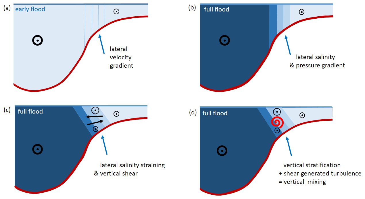
Figure 14 Sketch for explaining the effect of the channel-shoal transition on estuarine mixing during flood. The colour scaling indicates salinity, with dark blue colours representing high salinities. (a) early flood, when for simplicity no lateral salinity gradients are assumed; (b) full flood, generation of lateral salinity and thus density gradients due to differential advection; (c) full flood, lateral exchange flow driven by lateral density gradients leading to vertical stratification; (d) vertical shear generates small-scale turbulence which in concert with vertical stratification leads to vertical mixing.
4.2.2 Mixing at fronts
Bathymetrical bumps and lateral constrictions in a tidal channel in conjunction with tidal flow and longitudinal salinity gradients can lead to frontogenesis in estuaries (Geyer and Ralston, 2015) as well as increased mixing. The principle of this process is sketched in Fig. 15 for the example of an ebb current: Assuming an initially vertically well-mixed estuary with equally-spaced vertical isohaline surfaces, a sheared ebb current over a bathymetrical bump and a zone of weak recirculation downstream of the bump (Fig. 15a), the isohalines will be strained differentially. Over flat bathymetry, the classical ebb straining described by Simpson et al. (1990) will occur, leading to increased mixing (Sect. 4.1.1, and left side of Fig. 15b). On the lee side of the bump, where the ebb flow is partially blocked near the bed, the down-estuary advection of the isohalines is reduced or inverted while it is increased near the surface. This situation leads to a near-bottom retention of saline water on the lee side of the bump and thus to increased salt stratification. At the same time, the recirculation velocity near the bed and thus the vertical shear on the lee side of the bump will increase due to the backward slope of the strongly stratified isohalines. Increased shear, in turn, leads to increased turbulence production which in concert with strong stratification finally leads to strongly increased mixing. In their model simulations of the Hudson River estuary, Geyer and Ralston (2015) show that the composite Froude number (Armi and Farmer, 1986) in the frontal zone becomes supercritical in a similar way as was observed offshore of the lift-off point of a river plume at the mouth of an estuary (Horner-Devine et al., 2015). Mixing hotspots related to bathymetric bumps in tidal channels are also visible in model simulations for the Hudson River estuary (Geyer and Ralston, 2015; Warner et al., 2020).
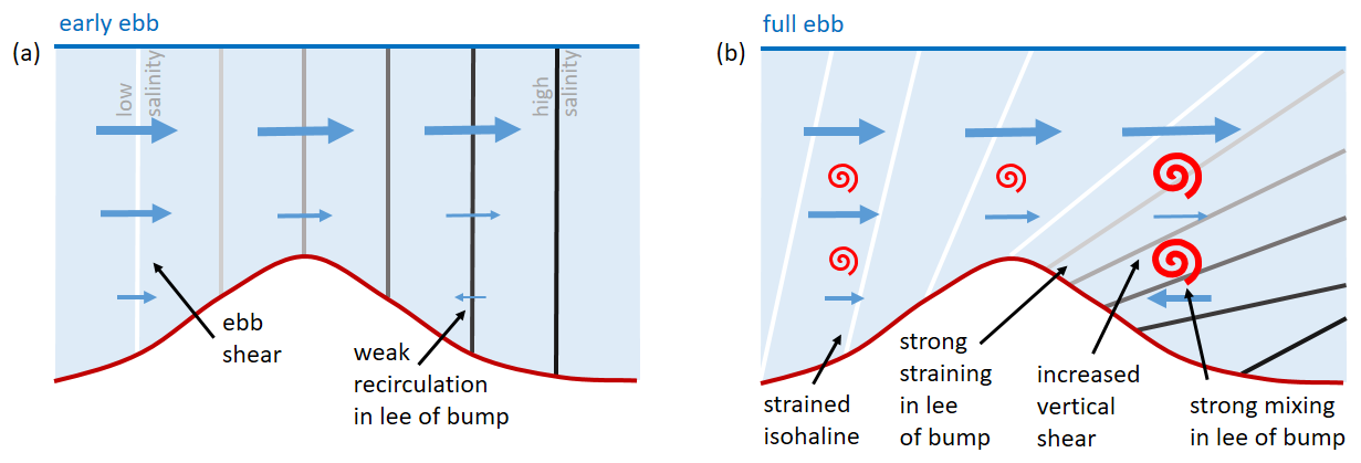
Figure 15 Sketch explaining the effect of along-channel bathymetric bumps on increased mixing during ebb. (a) The vertical lines represent isohalines, with light grey shading indicating lower and dark grey shading indicating greater salinity. During this phase of early ebb, the salinity field is still assumed to be vertically well-mixed. The arrows represent horizontal flow velocity, showing some weak recirculation in lee of the bathymetric bump; (b) due to strong shear and blocking of the flow, the salinity field is most strongly strained in lee of the bump. The combination of strong shear-generated turbulence and strong salinity stratification then leads to a hotspot of vertical salt mixing.
A realistic example of frontal mixing comes from a numerical model representation of the partially mixed James River estuary (Fig. 16). This estuary has two pronounced constrictions, one at km 18, and the other at the mouth at km 30. The expansions on the seaward (right) side of these constrictions result in steep upward tilt of the isopycnals due to the supercritical hydraulic response to the expansions (Geyer et al., 2017). These steeply sloping isopcnals are associated with strong horizontal and vertical salinity gradients, i.e., frontal conditions. At the time of maximum ebb, mixing (as quantified by ) shows a pronounced maximum along each of the frontal zones. The energy for mixing along these frontal zones does not come from the bottom boundary layer, but rather from the baroclinic shear associated with the steeply sloping pycnocline. That strong shear also maintains the strong stratification via longitudinal straining of the horizontal salinity gradient. An observational example of the same phenomenon is discussed in Sect. 5.1 and illustrated in Fig. 17.
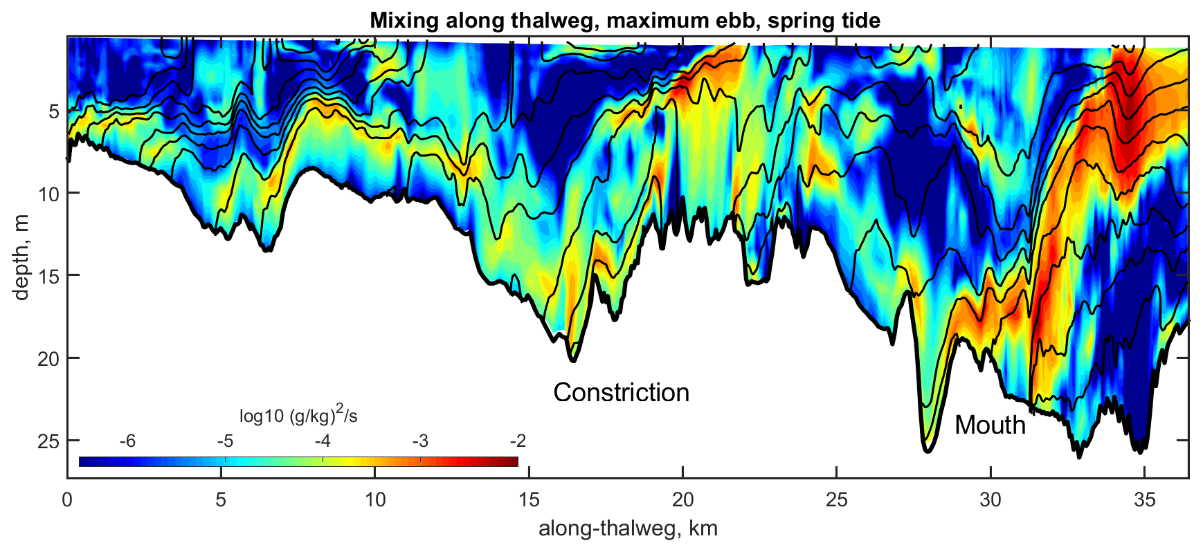
Figure 16Realistic numerical simulation of conditions along the thalweg of the James River estuary during maximum ebb of spring tide, under moderate river discharge conditions, illustrating frontal zones with intensified mixing. The vertical component of the local mixing rate, , is shown as colour scale. The along-estuary salinity distribution is indicated by black contours (contour interval 1 g kg−1).
5.1 Observational methods
Direct field measurements of the mixing of salt in estuaries is impractical, due to the microscopic scales at which the dissipation of salinity variance occurs, see Sect. 2.1. The turbulent motions that drive mixing can be resolved however, and numerous field investigations have quantified mixing based on measurements of turbulent motions at scales from metres to centimetres, then using theoretical arguments to relate the observable characteristics of the turbulence with either the mixing χs or the diahaline turbulent salt flux jdia,z. A common approach is to use the relationship between the eddy diffusion coefficient for mass Kv and turbulent kinetic energy dissipation rate ε,
as proposed by Osborn (1980), where Rf is the flux Richardson number and N is the buoyancy frequency. With an estimate of Kv and a local measure of the vertical salinity gradient , the vertical turbulent salt flux jdia,z and the salinity variance dissipation χs are readily estimated, see Eqs. (10) and (26). Peters and Bokhorst (2000, 2001) pioneered the use of a free-falling shear probe in an estuary for the purpose of quantifying mixing; since then this method has been followed in a variety of estuarine settings (Rippeth et al., 2001; Becherer et al., 2011; Ross et al., 2019; Huguenard et al., 2019; Reese et al., 2026). This method is challenging for measuring turbulence near the bottom, due to the risk of smashing the delicate shear probe into the bottom. An alternative method is the estimation of the dissipation rate ε based on the inertial-subrange velocity spectrum measured by a turbulence-resolving current meter (Trowbridge et al., 1999; Giddings et al., 2011). A related methodology pioneered by Gargett (1994), and applied by Stacey et al. (1999), Lu and Lueck (1999) and Giddings et al. (2011) among others is to use an Acoustic Doppler Current Profiler (ADCP) to obtain a direct measurement of the Reynolds stress , then in combination with a measure of the vertical shear to estimate eddy viscosity Av, and then to infer the eddy diffusivity Kv and the mixing rate χs.
These methods are most effective in weak stratification conditions, when dissipation rates tend to be high and the turbulent length scale is readily resolved by the sensor. As stratification gets stronger, however, the scales of turbulent motions decrease, as scaled by the Ozmidov scale
making it harder to obtain a reliable estimate of ε. More problematical is that the estimation of mixing χs depends on the square of the local salinity gradient, see Eq. (9), which itself is a challenging quantity to measure at the small vertical scales relevant to turbulence within a stratified environment.
Micro-conductivity sensors provide a means of resolving the salinity gradient and associated overturns at scales relevant to the characterization of turbulent motions (Peters and Bokhorst, 2001). The Thorpe overturn scale LT (Thorpe, 1977) provides an alternative means of estimating the turbulent dissipation rate:
as shown by Peters (1997) in his turbulence measurements in the Hudson River estuary. It is particularly useful in the stratified interior, where the small vertical scales of turbulence make other methods of estimating ε more difficult (Etemad-Shahidi and Imberger, 2002; McPherson et al., 2019).
All of the above methods depend on a turbulence closure assumption as well as an estimate of mixing efficiency to link the dissipation rate ε to the actual mixing of salt, χs. The use of micro-conductivity sensors offers a more direct approach to estimating the mixing of salt. Following Holleman et al. (2016), high-frequency micro-conductivity time series measurements can resolve the inertial subrange and the viscous-convective subrange of the salinity variance spectrum
where Sss is the power spectral density of salinity variance, b0=0.4 is the Kolmogorov constant for scalar variance, 𝒦 is the wave number and is the Kolmogorov wave number, with the molecular viscosity ν. Note that the last term in Eq. (41) resolves the transition from the inertial subrange to the viscous-convective subrange at length-scales of . As long as the height of the spectrum within either the inertial or viscous-convective subrange can be estimated, Eq. (41) can be used in combination with an estimate of ε to estimate mixing, i.e., the dissipation of salinity variance χs, without relying on turbulence closure assumptions. Moreover, the formula depends only weakly on the estimate of ε, which is often hard to estimate accurately in the stratified turbulent regime. Holleman et al. (2016) used this method to estimate mixing rates in the highly stratified Connecticut River estuary. Their analysis demonstrated peak values of χs in the pycnocline in association with intense shear instability during ebb tide (Fig. 17).
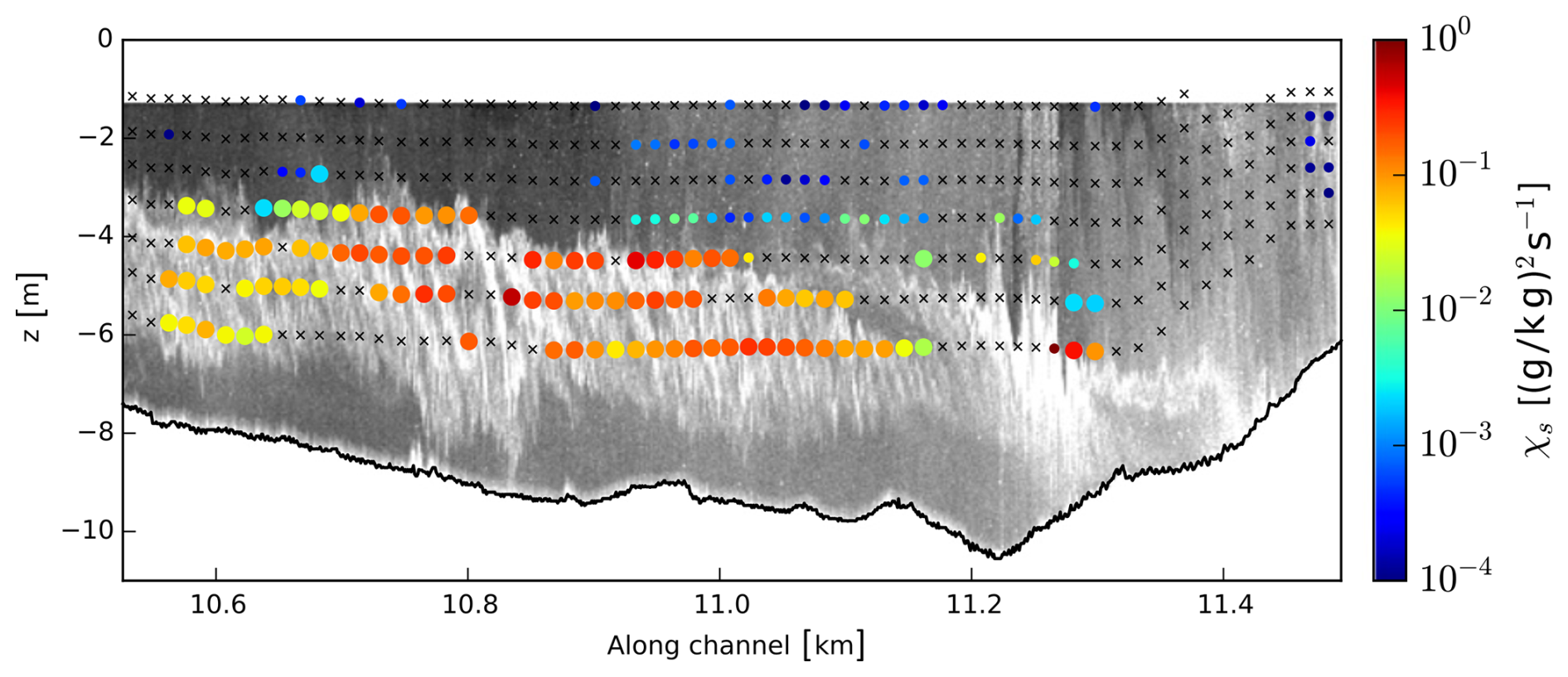
Figure 17Spatial distribution of χs (coloured dots) in the stratified shear layer of the early ebb in the Connecticut River estuary, estimated from combined observations by a string of Acoustic Doppler Velocimetres (ADVs) and microconductivity probes. The crosses are locations where values of χs could not be reliably estimated. The grey scales in the background indicate the intensity of acoustic backscatter. This figure has been taken from Holleman et al. (2016).
Acoustic backscatter also provides a more direct means of estimating mixing, as demonstrated by Lavery et al. (2013). Using a broadband array of echo sounders, Lavery et al. (2013) demonstrated that the observed scattering in the pycnocline of the Connecticut River estuary has a spectral slope consistent with the viscous-convective subrange. Other scatterers, such as fish, bubbles and sediment, have distinctly different spectral slopes. If the stratification is strong enough and other scatterers do not overwhelm the signal, the acoustic backscatter intensity can be used as a nearly direct measure of χs. While the signal-to-noise ratio of the acoustic amplitude does not offer the same precision as microstructure measurements, it produces remarkable spatial resolution, as demonstrated by acoustic measurements within a train of Kelvin-Helmholz instabililities in the Connecticut River estuary (Fig. 18). Based on the evidence provided by the analysis of Lavery et al. (2013), echo-sounding imagery can be used to identify regions of intense mixing, even if the actual magnitude of χs cannot be quantified.
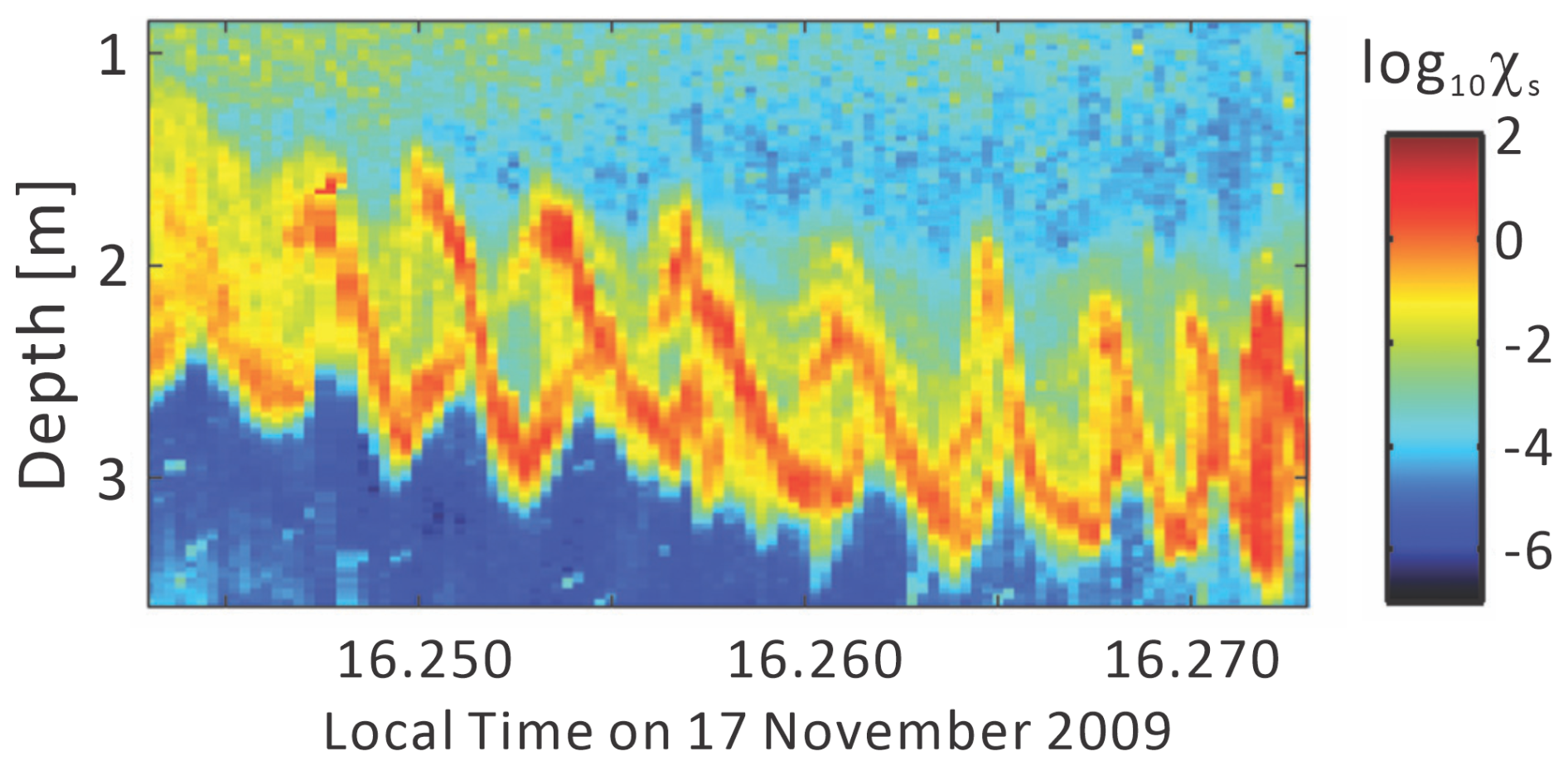
Figure 18Kelvin-Helmholtz instabilities in the Connecticut River estuary. The colour shading shows the decadal logarithm of the salinity mixing χs, estimated from acoustic backscatter measurements. This figure has been taken from Lavery et al. (2013).
5.2 Numerical modelling techniques
Since direct observations of turbulent properties in estuaries are very tedious and noisy (see the discussion in Sect. 2.1), the analysis of mixing in estuaries largely relies on numerical models. The advantage of numerical models is certainly their coverage of the entire four-dimensional estuarine space (three spatial directions and time), whereas observations can only sparsely cover this space. However, to ensure that the numerical model results sufficiently represent real estuaries, several measures need to be taken: besides realistic input data into the model (such as bathymetry, open boundary conditions, meteorological forcing) and a thorough validation using observational data, the numerical model itself must be physically sound and numerically accurate. There is an extensive body of literature addressing these two topics (Griffies, 2004; Umlauf and Burchard, 2005; Shchepetkin and McWilliams, 2005; Zhang et al., 2016; Klingbeil et al., 2018). Here, we will present in more detail two aspects which are key to the proper assessment of mixing in estuaries: turbulence closure modelling (Sect. 5.2.1) and numerical mixing analysis (Sect. 5.2.2).
5.2.1 Turbulence closure modelling
The starting point of turbulence closures are the fundamental laws of momentum, mass and energy conservation from which transport equations based on molecular viscosities and diffusivities can be derived, see e.g. the molecular salinity equation Eq. (2). Applying the Reynolds decomposition (see Lesieur, 2008, and the discussion in Sect. 2.1) leads to transport equations for Reynolds-averaged variables, see e.g. the salinity equation Eq. (4), which include unknown second moments such as the vertical turbulent salt flux . In a similar manner, exact transport equations can be derived for those second moments, which however would include unknown third moments, and so forth. This infinite series of unclosed higher and higher order equations establishes the turbulence closure problem. An example for a second-moment transport equation ( in this case) is Eq. (5) which includes among others the vertical turbulent transport of the micro-structure salinity variance as a third moment. Second-moment closures use parameterisations for all unknown third moments, such that the system of second-moment transport equations is closed. To substantially simplify the solution, equilibrium assumptions are made for most second moments in such a way that the sum of the transport divergence and the time change are set to zero. For the example of the micro-structure variance equation Eq. (5), this leads to the equality of stirring and mixing (Ps=χs), see also the discussion in Sect. 2.1.
A central element of turbulence closures is the eddy diffusivity assumption Eq. (7), relating turbulent tracer fluxes to Reynolds-averaged tracer gradients, with the eddy diffusivity as a factor of proportionality, leading to the principle of down-gradient turbulent tracer fluxes. Similar assumptions are made for momentum and turbulent quantities. The eddy diffusivities include the entire second-moment closure. For the key quantity of the turbulent kinetic energy (), a budget equation is generally solved with shear production as source term and dissipation of TKE into heat as sink term. For stable stratification, turbulence leads to mixing as well as negative buoyancy production, which leads to an increase of local potential energy and acts as a further TKE sink term. For estuarine numerical modelling, the use of so-called two-equation turbulence closure models has become a good compromise between efficiency and accuracy (Warner et al., 2005a). In such models, the first equation generally is the budget-equation for the TKE, while the second equation is related to the length scale of turbulence, such as the dissipation rate of TKE, ε (the k-ε model), or the turbulence frequency, (the k-ω model). If properly calibrated, these different versions of length-scale related equations perform similarly (Warner et al., 2005b). The most important aspect of the calibration is to ensure the quantitatively correct damping of vertical turbulent mixing caused by stable stratification. The principles of this calibration process are explained in Appendix E. In essence, the steady-state gradient Richardson number is set to the value of Rist=0.25 such that for stronger stratification (Ri>Rist), turbulence is suppressed and for weaker stratification it is enhanced. A properly calibrated turbulence closure model does also reproduce the canonical values of mixing efficiency Γ≈0.2 and the steady-state flux Richardson number Rfst≈0.15 (Osborn, 1980). It should be noted that these values would only be reached in numerical models for so-called stationary homogeneous shear layers where production and destruction of TKE are balanced. In cases of strong temporal variability or locations with a substantial vertical turbulent transport of TKE (such as in active entrainment layers), significant deviations can occur (see the discussion by Holleman et al., 2016).
5.2.2 Numerical mixing analysis
Although the numerical mixing in the model of the Elbe River estuary is relatively small (see Figs. 4 and 8), it can be of considerable size in other estuarine models (Ralston et al., 2017; Henell et al., 2023). Therefore, the quantification of numerical mixing is discussed here. As demonstrated in the previous sections, the comparison of analytically derived mixing relations with diagnosed mixing from numerical simulations requires the quantification of the total variance decay experienced by a tracer in the numerical model. This does not only consist of contributions from the parameterised turbulence closure (physical mixing), but also from the discretisation of the tracer advection operator (spurious numerical mixing; Griffies et al., 2000). It is assumed that the tracer advection discretisation is conservative, monotone (in the sense that it does not generate wiggles and new tracer maxima and minima) and weakly diffusive. Many advection schemes with these properties have been developed such as the FCT (Flux-Corrected Transport) schemes (Zalesak, 1979), TVD (Total Variation Diminishing) schemes (Pietrzak, 1998) and the MPDATA (Multidimensional Positive Definite Advection Transport Algorithm) schemes (Smolarkiewicz, 2006). They all use some degree of implicit diffusion to ensure monotonicity.
In many model applications, numerical mixing has been found to explain a large portion of the total (physical plus numerical) mixing. High values of numerical mixing of typically 50 % have been found for the Baltic Sea (Hofmeister et al., 2011) and the Puget Sound (Broatch and MacCready, 2022), while Li et al. (2018) report about 33 % of numerical mixing for their simulation of the Changjiang River estuary. Low numerical mixing has been seen for simulations with high explicit horizontal diffusivity (Reese et al., 2024, for the Elbe River estuary) or for idealised estuarine models (MacCready et al., 2018). To account for the role of numerical mixing and to evaluate measures for its reduction, numerical mixing analysis methods have been developed (Burchard and Rennau, 2008; Klingbeil et al., 2014; Schlichting et al., 2023; Banerjee et al., 2024). Here, we first briefly describe general methods to quantify physical and numerical mixing in ocean models, before we give recommendations on how to reduce numerical mixing (see below).
Methods to quantify numerical mixing
To demonstrate methods to discriminate between physical and numerical mixing and to accurately quantify their sum, we give a detailed one-dimensional example of an advection-diffusion equation in Appendix F, including its discretisation (Appendix F1), the derivation of the mixing analysis (Appendix F2), a stationary solution of the one-dimensional advection-diffusion equation (Appendix F3) and the derivation of its analytical solution (Appendix F4). For this analysis, a first-order upstream (FOU) method is used as an example because it allows for an explicit discretisation of the physical and numerical mixing. Since the FOU scheme for advection shown in Eq. (F3) is inherently diffusive, it is generally not used in ocean models. Instead, mostly non-linear schemes are used for which the spurious numerical variance decay cannot be analytically derived. To separate between physical and numerical mixing, it is convenient to carry out the advection and diffusion discretisation in different steps, as an operational-split method. After the advection step, the numerical mixing is diagnosed, and after the diffusion step, the physical mixing is calculated. It is also possible to further separate the numerical and physical mixing into horizontal and vertical contributions. Different methods of numerical mixing quantification have been proposed for the pure advection step. Since the advection equation for the squared tracer, Eq. (F2) for Kh=0, is equivalent to the advection equation for the tracer itself, Eq. (F1) for Kh=0, Burchard and Rennau (2008) proposed to additionally carry out an advection step for the squared tracer (which should conserve the squared tracer) and to subtract from it the square of the advected tracer, Eq. (F1), which reduces the squared tracer. This difference should be a good estimate for the variance reduction in a particular grid point during a particular time step. Division by the time step Δt should give the local numerical variance decay (or mixing). As an alternative, Klingbeil et al. (2014) proposed to calculate the left-hand side (time derivative and advection term) of the diagnostic tracer-square advection equation as an estimate for the right-hand side (which should be the numerical mixing). Yet another method has recently been proposed by Banerjee et al. (2024). All three methods are equivalent when integrated over a larger area, and differences do only show up in the local distribution of the numerical mixing. An accurate numerical mixing quantification requires the direct implementation of the analysis into the numerical model code, since analysing numerical mixing from model output even at high output frequency has proven quite inaccurate (Schlichting et al., 2023).
There are alternative diagnostic methods to quantify numerical mixing, however not in terms of variance decay (Gibson et al., 2017; Holmes et al., 2021; Drake et al., 2025).
Measures to reduce numerical mixing
Generally, a finer resolution should lead to a reduction of numerical mixing. However, Burchard and Rennau (2008) showed that this might not be very efficient, since for an idealised example a grid-refinement by a factor of nine in the horizontal direction and by a factor of four in vertical direction (equivalent to a 144-fold increase in computational resources) led to a reduction of numerical mixing by less than a factor of two. More promising is the better alignment of grid layers with isopycnals, or adding a Lagrangean type of vertical grid motion, to reduce vertical advection with respect to moving coordinate layers. Specifically, vertically adaptive coordinates proved to significantly reduce numerical mixing (Hofmeister et al., 2011; Gräwe et al., 2015). A further reduction of numerical mixing can be achieved by aligning the horizontal grid with the major tidal flow directions. The present Elbe River estuary model (adopted from Reese et al., 2026) as well as the Weser River estuary model by Rummel et al. (2025) align the curvilinear grid with the dredged navigational channel and not, as typically done, with the lateral shoreline. This reduces numerical mixing because in estuaries lateral salinity gradients are generally much larger than longitudinal ones, such that these specially constructed horizontal coordinates align with those gradients which then do not have to be advected with the along-estuary flow across grid interfaces.
Numerical mixing is a fact in all numerical model applications and cannot be avoided. It is therefore essential to quantify its contribution to the tracer distribution, which is the result of the sum of intended physical and unintended numerical mixing. Intentionally reducing physical mixing would be one way to obtain realistic total mixing. This has been impressively demonstrated by Ralston et al. (2017) who in a model application to the Connecticut River estuary reduced the physical mixing by reducing the steady-state Richardson number Rist from the canonical value of 0.25 (see Sect. 5.2.1) to a very low value of 0.1. By doing so, they increased the numerical mixing from 50 % to 66 %, but reduced the total mixing such that the resulting salinity structure was more realistic. Such measures should however be handled with care since the numerical mixing generally has a different spatial and temporal distribution than the physical mixing (Klingbeil et al., 2014; Henell et al., 2023).
As reviewed in this paper, the work of past decades nowadays provides a consistent theoretical framework for estuarine mixing, the foundations of which have been laid in the early work by Knudsen (1900) and Walin (1977). Although their work did not explicitly define and quantify mixing, mixing theories are conveniently founded on their frameworks. In agreement with turbulence theory (Osborn and Cox, 1972; Mellor and Yamada, 1974), local mixing of a certain tracer is defined as the dissipation rate of the local variance of this tracer, χs, see Eqs. (9) and (B1) and Burchard and Rennau (2008). Estuarine mixing 𝕄 itself is then the integral of χs over estuarine volumes averaged over a certain period of time (e.g., the spring-neap cycle). Relating these definitions to bulk forcing parameters for the estuaries leads to the Knudsen mixing law Eq. (21) when the estuary is bounded by a fixed transect (MacCready et al., 2018) or to the universal law of estuarine mixing Eq. (32) when the estuary is bounded by a moving isohaline (Burchard, 2020). Therefore, to understand the estuarine mixing 𝕄, its temporal and spatial composition by means of the local variance decay χs has to be studied. In a few cases, this was achieved through observations (e.g., Lavery et al., 2013; Holleman et al., 2016), but is more typically done with realistic numerical models of estuaries (e.g., Warner et al., 2020; Reese et al., 2024). These models are consistent with the mixing theories only if numerical mixing due to the discretisation of the tracer advection terms is included (e.g., Li et al., 2022). Using these observations and modelling techniques, the major mixing processes in some example estuaries are now understood, see e.g. Warner et al. (2020) for the Hudson River estuary, Broatch and MacCready (2022) for the Salish Sea, Henell et al. (2023) for the Baltic Sea and Reese et al. (2026) for the Elbe River estuary.
Due to its high relevance for the understanding of estuarine dynamics and its socio-economical and ecological consequences, the research on estuarine mixing will continue. More studies for other estuaries will certainly come, most probably resulting in a different weighting of the most relevant mixing processes, maybe even describing new processes. But apart from that, the future of estuarine mixing research will likely be dominated by the technological progress that allows for ever finer-resolved, more efficient numerical modelling down to smaller and smaller scales. Here, we discuss in detail where, and to which extent, we see potential for such progress.
6.1 Increased computational resources
It is expected that the trend of ever-increasing computational resources will continue. As an important development, the ongoing replacement of the more traditional Central Processing Units (CPUs) by modern Graphics Processing Units (GPUs) will improve the overall computational efficiency. As computational codes for coastal ocean models will become available for GPUs, this increase in computational power can be used for finer resolution models, longer simulation periods or larger model domains. Finer resolution models would be able to resolve further processes of estuarine mixing with more accuracy, such as smaller-scale topographic effects. Specifically, consequences of coastal engineering such as dredging and dam-building, which are commonly under-resolved in contemporary numerical simulations, could be reproduced more realistically. Today, multi-decadal simulations of well-resolved estuaries are hardly feasible. Such longer simulation periods could, however, be used to better reproduce interannual variability and consequences of long-term trends such as sea-level rise and changes in precipitation and evaporation patterns. Larger model domains could help to include more of the tidal or non-tidal parts of rivers or larger portions of the adjacent ocean including the river plume. It has been shown that the universal law of estuarine mixing Eq. (33) is only valid for isohaline surfaces that do not leave the model domain. On the other hand, isohaline theory does not distinguish between estuarine and river plume mixing, and often the transition between the two cannot be seen from model topography and coastlines. Therefore, it is desirable to simulate the entire river-estuary-plume region within a single model setup. Similarly, the confluence of multiple estuaries and river plumes could be simulated at fine resolution when computational resources further improve.
6.2 Large Eddy Simulation modelling
More powerful computer resources could also allow for models with improved model physics, such as using higher-order turbulence parameterisations or the application of Large-Eddy Simulation (LES) models. Both improvements would have a direct effect on the computation of mixing. One example for higher-order turbulence closure models could be the use of non-local models that do not enforce the down-gradient assumption of turbulent fluxes (see the recent study by Legay et al., 2025). Furthermore, parameterisations of Langmuir Turbulence which potentially affects estuarine mixing in the presence of wind waves could be added (Harcourt, 2015). The application of LES models to estuaries would mean that the most energetic turbulent eddies could be resolved instead of being parameterised by turbulence closure models. Then, only the small-scale mixing would need to be parameterised, for which generally relatively simple closures should be sufficient. A further advantage of LES models over classical coastal ocean models is their non-hydrostatic pressure calculation which would allow for the reproduction of non-hydrostatic effects such as internal lee wave generation (Skyllingstad and Wijesekera, 2004), generation of interfacial waves at pycnoclines when the surface and the bottom boundary layers interact (Yan et al., 2022) or Langmuir Circulation effects in shallow coastal waters (Wang et al., 2022). Two specific LES model applications have been reported by Li et al. (2008) and Li et al. (2010) who calculated a tidal water-column setup with periodic boundary conditions in both horizontal directions. So far, no further estuarine LES applications have been published. Specifically efficient LES model codes such as Oceananigans (Ramadhan et al., 2020) that can be executed on GPUs open vast possibilities of coastal (see the recent study by Huang et al., 2025) and estuarine LES applications in the future, starting with idealised setups, but also with the future potential to simulate estuarine dynamics over more realistic topographies.
6.3 Water Mass Transformation theory
The concept of Water Mass Transformation (WMT) has been strongly extended in recent years (see, e.g., Hieronymus et al., 2014; Groeskamp et al., 2019). Such multi-dimensional WMT concepts using other constituents in addition to salinity, such as temperature or biogeochemical tracer concentrations, are typically applied to large-scale ocean problems. Estuarine applications have yet to be created, but could give insight where, for example, temperature plays an important role in addition to salinity, such as shown for the Arctic Ocean (Pemberton et al., 2015), the Persian Gulf (Lorenz et al., 2020) or the Baltic Sea (Henell et al., 2023).
6.4 Machine Learning
Finally, applications of Machine Learning (ML) have entered all fields of oceanography, including coastal and estuarine research. Typical estuarine applications would comprise the calculation of river discharge from meteorological data (Börgel et al., 2025) or the estimation of the salt intrusion length inside estuaries (Rummel et al., 2025). It is not yet obvious in which way fast, efficient and well-trained ML algorithms could be exploited to support research on estuarine mixing, but it can certainly be expected that ML applications will soon extend our toolkit in addition to numerical modelling and observational methods.
The effects of stirring and mixing in a fluid subject to molecular diffusion are explained here quantitatively by means of a simple analytical example. We assume a fluid in a glass beaker of 0.1 m depth and a cross-sectional area of 0.01 m2, thus containing 1 L of fluid. Imagine our beaker initially contains salty water underlaying freshwater with a smooth transition in between, with a horizontally homogeneous distribution such that they only depend on the vertical coordinate z and time t. The vertical diffusive spreading of the salinity in our beaker would then be described by the classical one-dimensional diffusion equation of the form
with m2 s−1 denoting the molecular diffusivity of salt. Let us assume an initial salinity distribution of the form
with the maximum salinity g kg−1 where n is a positive integer, and D the thickness of the fluid inside the beaker. For n=1, the fluid is unstirred, and we only have a single layer of salty water underneath the freshwater with mixed conditions in between (see Fig. 1a). Increasing n may be viewed as a simple model for a stirring process that creates an increasing number of interfaces between salty and fresh water. For n=30 (Fig. 1b), the stirring process has created 30 such interfaces, and for n=90 (Fig. 1c), 90 interfaces can be defined. It should be clear that in a real beaker, the stirring process induces salinity patches and streaks that are highly distorted and three-dimensional. Nevertheless, our simple one-dimensional model is sufficient to illustrate the basic effects of stirring and mixing as shown in the following.
To investigate the temporal evolution of the salinity layers as a result of mixing, we insert an ansatz of the form
into Eq. (A1), where a(t) denotes the dimensionless amplitude of the salinity with . This yields a differential equation of the form
where combines all parameters of the problem. The solution of Eq. (A4) is of the form
which reveals that τ plays the role of a mixing time scale.
The blue lines shown in Fig. 1 (see the figure caption for the parameters chosen) illustrate the behaviour of the solution found above for different values of n. For n=1 (no stirring, Fig. 1a) the effect of mixing is seen to be negligible after a period of ten minutes. If some gentle stirring is applied (figuratively using the spoon) such that n is increased to 30, considerable mixing effects can be seen already after 10 min (Fig. 1b). Only intensive stirring (n=90) leads to the desired result of (almost) complete mixing within a reasonable amount of time (Fig. 1c). For the parameters chosen, the mixing time scale is about τ=17 000 min for the case of no stirring (n=1), about τ=19 min for little stirring (n=30), and about τ=2 min for strong stirring (n=90).
This appendix introduces some Reynolds-averaged salinity-variance or salinity-square equations to demonstrate the function of the salinity variance decay χs as sink term. Based on Eq. (8) and using Eq. (9), the salinity variance equation with the local variance per unit volume and the volume-averaged salinity is of the following form:
where the advective and diffusive flux divergences conservatively re-distribute local variance. Mixing χs is the sink term for the local variance. An extra term due to the non-constant volume-averaged salinity is included in the change term (MacCready et al., 2018, see Burchard et al. (2018b) for hints to the derivation). The variance budget of the entire estuary results from integration of Eq. (B1) over the volume of the estuary:
(MacCready et al., 2018; Burchard et al., 2019), where A is the boundary of the estuary towards the river and the ocean, u is the velocity vector at the open boundary and dA is the normal vector orthogonal to the area element A pointing out of the estuary, see details in Li et al. (2018). While the volume integrated mixing is the only sink term in Eq. (B2), an explicit source does not exist. Instead variance may enter the estuary via the boundary transport term as freshwater from the river and as saline water from the adjacent coastal ocean.
Inserting Eq. (7) into Eq. (6), or multiplying the salinity budget equation Eq. (8) by 2s, we obtain a budget equation for the squared salinity, which has the same mixing term as the local variance equation Eq. (B1):
which is the parameterised version of Eq. (6). Often, it is more handy to diagnose the budget of the squared salinity Eq. (B3) rather than the local variance Eq. (B1), since the time-variable volume-averaged salinity does not need to be considered.
C1 Study region
The Elbe River estuary is located in northern Germany and extends over 150 km from a weir south of Hamburg to the German Bight in the North Sea. It is an M2-dominated, mesotidal estuary at a mean tidal range of 3.0 to 3.5 m (Boehlich and Strotmann, 2008). The tidal signal is further modified throughout the spring-neap cycle. Its broad salinity range (0.5 to >30 g kg−1 within the model domain), medium discharge intensity of about 800 m3 s−1 on a multi-decadal average (Strotmann, 2017), and relatively simple, funnel-shaped, single-channel geometry make this estuary an ideal example for the illustration of basic estuarine mixing dynamics. Further, the navigational channel is subject to intensive dredging measures, comparable to other estuaries under high anthropogenic maintenance, and surrounded by extensive tidal flats.
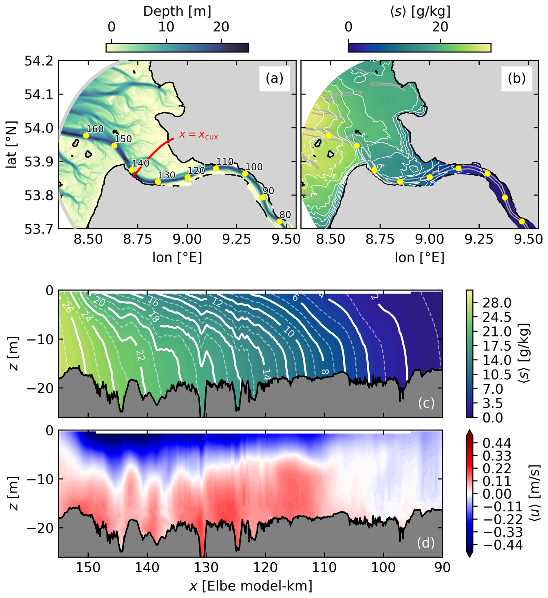
Figure C1Overview of the numerical simulation of the Elbe River estuary. (a) Downstream section of the setup topography, showing the open boundary in the German Bight as a bold grey line, the distance from the upstream boundary as yellow dots in km, and the location of the cross-channel transect used for the analysis in Fig. 2 as a red line. (b) Average surface salinity. White lines indicate even salinities. (c) Average salinity along the thalweg of the navigational channel. Solid (dashed) white lines indicate even (odd) salinities. (d) Estuarine circulation in terms of the tidally averaged along-channel velocity 〈u〉 along the thalweg of the navigational channel, where red shading indicates an inflow into the estuary and blue shading indicates an outflow towards the German Bight. In (b)–(d), the properties have been averaged for the full month of April 2024.
The Elbe is a partially mixed estuary with a medium stratification intensity as shown for the analysis period of April 2024 in Fig. C1b, c, where the spring-neap averaged surface to bottom salinity difference amounts to up to 6–7 g kg−1, and the salt intrusion reaches more than 50 km up-estuary. It displays a clear two-layer exchange flow pattern (see Fig. C1d).
A more detailed description of the Elbe River estuary can be found in Burchard et al. (2004), Reese et al. (2024), and Burchard et al. (2025).
C2 Numerical model and setup
The three-dimensional numerical model data used for all Elbe River examples in this paper was created with the General Estuarine Transport Model (GETM; Burchard and Bolding, 2002; Klingbeil and Burchard, 2013). For turbulence closure, GETM is coupled to the General Ocean Turbulence Model (GOTM; Burchard et al., 1999; Li et al., 2021), here using a second-order, algebraic closure for a k-ε parameterization (Umlauf and Burchard, 2005).
The specific Elbe River estuary setup used here is identical to the setup presented in Reese et al. (2026) with a high horizontal (2404×397 cells with a mean resolution of 80 m in along-channel direction and 98 m in cross-channel direction) and vertical (40 adaptive layers) grid resolution. It covers the year 2024 and uses a curvilinear grid with thalweg-following and cross-channel grid lines, resulting in horizontal grid cells of variable size, where the finest resolution is achieved within the navigational channel. The model domain is limited in upstream direction by the location of a weir that marks the end of the upstream tidal intrusion, and in downstream direction by an open boundary within the German Bight.
Overall, the Elbe River setup uses a realistic forcing. This includes initial distributions for temperature and salinity as well as tidal elevations and vertical temperature and salinity profiles along the open boundary (E.U. Copernicus Marine Service, 2024), the daily-averaged freshwater discharge at the upstream end of the model domain (Wasserstraßen- und Schifffahrtsamt Magdeburg, 2024) at a constant salinity of 0.5 g kg−1, and a 1 km-resolved meteorological forcing (Norwegian Meteorological Institute, 2024).
A full setup description along with a process-oriented model performance evaluation can be found in Reese et al. (2026).
Neglecting horizontal turbulent fluxes, the salinity equation Eq. (8) can also be formulated as
Assuming a stable salinity stratification with , for every isohaline the vertical position can be given by such that Eq. (D1) can be multiplied by and time-averaged on a fixed isohaline, 〈〉s to yield
and udia,z (the diahaline velocity per unit horizontal area) can be obtained from
Note that the diahaline fluxes udia,z and jdia,z are defined positive upwards here, whereas they are usually defined positive up-gradient in the literature. For almost flat isohalines can be interpreted as the vertical velocity relative to the moving isohalines. Due to the neglect of horizontal turbulent fluxes, the diahaline diffusive salt flux per unit horizontal area jdia,z in Eq. (D2) is identical to the vertical turbulent salt flux. Henell et al. (2023) and Reese et al. (2024) demonstrated that relation Eq. (D2) approximately holds also in realistic estuarine cases where horizontal turbulent fluxes are present. Moreover, relation Eq. (D2) also holds for arbitrary salinity distributions including inversions, based on generalised definitions of udia,z and jdia,z (Klingbeil and Henell, 2023).
After carrying out a second-moment closure as briefly described in Sect. 5.2.1 and presented in more detail by Burchard and Bolding (2001) and Umlauf and Burchard (2005) and applying the boundary layer assumption (vertical gradients are much larger than horizontal gradients), the closure results in the down-gradient parameterisation of momentum,
with the eddy viscosity Av, and the down-gradient parameterisation for turbulent tracer flux Eq. (7), with the following relation for the eddy viscosity Av and the eddy diffusivity Kv:
with the non-dimensional stability functions cμ and depending in the case of quasi-equilibrium stability functions (Galperin et al., 1988) on the non-dimensional gradient-Richardson number Ri, the turbulent kinetic energy per unit mass, k, and its dissipation rate, ε. The definition of the gradient Richardson number
is given with the squared shear frequency , the squared vertical shear . The stability functions cμ and include the entire second-moment closure (Burchard and Bolding, 2001).
For the case of two-equation turbulence closure models the full transport equations for k and ε are calculated (Rodi, 1987). Instead of the dissipation rate equation, other length-scale related properties such as the turbulence frequency could be modelled, following the generic length scale (GLS) approach by Umlauf and Burchard (2003). The k-ε model, as it is typically used in three-dimensional coastal ocean models, is of the following form:
with the shear production , and the vertical buoyancy flux . In Eq. (E4), c1, c2, c3, σk and σε are empirical parameters. The horizontal diffusive transport of k and ε is generally ignored. To demonstrate how these two-equation turbulence closure models are calibrated to predict the correct response of mixing to stratification and shear, the transport equations for k and ε are analysed for homogenous shear-layers where the advective and diffusive transport-divergence terms vanish. Necessary conditions for equilibrium solutions of Eq. (E4) are found by setting the left-hand sides to zero, such that Eq. (E4) can be transformed to
with the steady-state gradient Richardson number Rist denoting the gradient Richardson number for the stationary solution. To obtain the result of Eq. (E5), first ε was eliminated. With the well-calibrated parameters c1=1.44 and c2=1.92 (Rodi, 1987) and Rist=0.25 (Schumann and Gerz, 1995) Eq. (E5) provides an implicit non-linear equation to calibrate c3 which determines the damping effect of stratification on turbulence (Burchard and Bolding, 2001). For the second-moment closure by Cheng et al. (2002) this leads to (Umlauf and Burchard, 2005). It can be shown that for a large gradient Richardson number with Ri>Rist turbulence is damped due to stable stratification and vice versa (Burchard and Bolding, 2001). This means that an increased steady-state gradient Richardson number with Rist>0.25 will lead to increased turbulence for a given Ri and vice versa (Umlauf and Burchard, 2005). This principle has been used by Ralston et al. (2017) to decrease physical mixing by substantially lowering Rist in order to account for the too high numerical mixing of an estuarine model, see Sect. 5.2.2. Interestingly, steady-state solutions of Eq. (E4) under the neglect of transport divergences are also provided by
For the settings of c1, c2 and c3 given above, a mixing efficiency of Γ=0.21 and a steady-state flux Richardson number of Rfst=0.17 result (both close to the generic values of Γ=0.2 and Rfst=0.15 by Osborn, 1980), see the derivations by Umlauf (2009).
F1 Discretisation of the one-dimensional advection-diffusion equation
To illustrate the quantification of physical and numerical mixing, the simple case of the one-dimensional advection-diffusion equation and its discretisation by means of a first-order upstream scheme for the advection term and a central-difference scheme for the diffusion term is examined here. The one-dimensional advection-diffusion equation is of the following form:
with the constant advection velocity u and the positive and constant physical diffusivity Kh>0. Multiplying Eq. (F1) by 2s results in the one-dimensional version of Eq. (B3):
with the physical mixing χs on the right-hand side as a sink term. For u>0, a straight-forward explicit-in-time discretisation for Eq. (F1) with constant time step Δt and constant spatial increment Δx is given by
with a first-order upstream discretisation for the advection term and a central-difference discretisation for the diffusion term. In Eq. (F3), the subscripts i indicate the spatial increment and the superscripts n indicate the number of the time step. For a negative velocity u<0, the upstream discretisation of the advection term would simply mean to exchange by . The scheme is numerically stable for a Courant number of and the diffusion number . Multiplication of Eq. (F3) by (equivalent to the multiplication of Eq. (F1) by 2s) and subsequent reorganisation results in a diagnostic equation for the advection and diffusion of s2, as reproduced by the discretisation of the advection-diffusion equation Eq. (F1):
where the second and third lines are the discrete physical mixing and the last line is the numerical mixing. A step-by-step derivation of Eq. (F4) is given in Sect. F2. The left-hand side of Eq. (F4) is the discretisation of the advection and diffusion of s2 and the first term on the right-hand side is a consistent discretisation of the physical mixing, where the non-dimensional numerical parameters μ and ν determine the weights for the composition of the discrete squared salinity gradient by means of the discrete values , and . Although this term partially depends on numerical parameters, we associate it with physical mixing, since it is proportional to the eddy diffusivity Kh. The second term on the right-hand side is a sink term for stable conditions with , and is therefore called the numerical mixing term (Burchard and Rennau, 2008). With the numerical diffusivity it has a similar structure as the physical mixing, being twice the diffusivity times the tracer-gradient square.
F2 Derivation of physical and numerical mixing for the one-dimensional advection-diffusion equation
Here we show the step-by-step calculation of the physical and numerical mixing for the advection-diffusion equation with first-order upstream (FOU) discretisation for advection and central difference discretisation for diffusion Eq. (F3), which is the starting point here:
Multiplication of Eq. (F5) by results in
where we mark changes from step to step by an underline. Substitution of
with the Courant number and the stability number for diffusion gives
Reordering gives
Adding on both sides
gives
Equation (F12) is the diagnostic discrete equation for the advection-diffusion equation of squared salinity, where the right-hand side shows the total discrete mixing, consisting of a discretisation of the physical mixing plus contributions from numerical mixing. To differentiate numerical and physical mixing, we split the right-hand side into a purely advective contribution (only containing and μ) and the remainder:
Noting that
and reformulating the purely advective term, we obtain
Now the right-hand side will be expressed as gradient-squared terms. This is simple for the advective term. For the diffusive term, we apply the following Ansatz to express it as a linear combination of the three possible discrete gradient-square terms:
Comparison of coefficients results in
with the solution
With this, Eq. (F15) can be expressed as
which can be reformulated as
and which is identical to Eq. (F4). It should be noted that for stationary problems (which must not depend on the time step Δt) such as the discrete solution of the exponential estuary in Appendic F3, the sum of all terms in Eq. (F20) containing one of the numerical parameters μ or ν is zero:
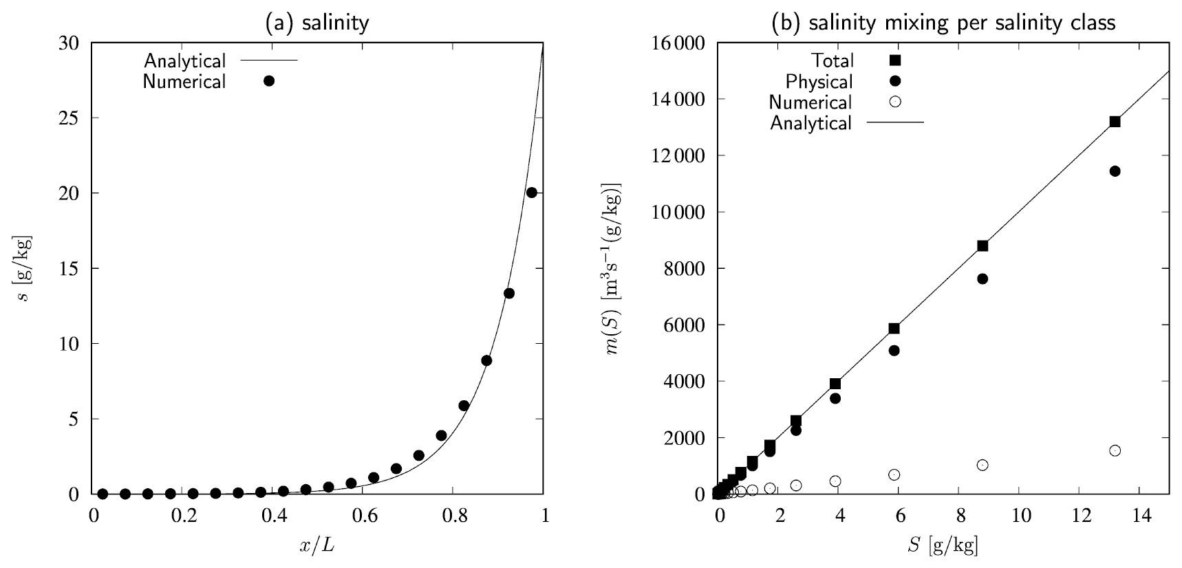
Figure F1Analytical and numerical solutions for the one-dimensional stationary estuary with run-off velocity u=0.05 m s−1, Kh=500 m2 s−1, L=100 km and A=10 000 m2 (such that the run-off is m3 s−1 and the river salinity is g kg−1). The numerical solution is carried out for equidistant spatial increments of . (a) Analytical solution Eq. (F23) and numerical solution (bullets) for salinity s as function of non-dimensional estuarine length . (b) Analytical solution Eq. (33) and numerical results for the salinity mixing per salinity class m(S): Total mixing (squares), physical mixing 𝕞phy,i (bullets) and numerical mixing 𝕞num,i (circles).
F3 One-dimensional stationary estuarine example
We demonstrate the distribution of physical and numerical mixing for a simple example of a one-dimensional stationary estuary of length L with constant cross-section A and constant discharge velocity u>0 (such that the river run-off is Qr=uA) and constant along-estuary diffusivity Kh>0, being slightly simplified from Burchard (2020). Under those circumstances, the stationary form of Eq. (F1) describes the balance,
of which the analytical solution for salinity is exponentially increasing from the river towards the ocean,
with the ocean salinity so at x=L and the river salinity at x=0. The universal law of estuarine mixing Eq. (33) can be directly derived from Eq. (F23), see Appendix F4 for details.
The analytical solution Eq. (F23) and a numerical solution, obtained by iterating Eq. (F3) into a stationary state, are given in Fig. F1a. Using equidistant spatial increments results in a good numerical representation of the analytical solution with some deviations at high salinities. The universal law of estuarine mixing Eq. (33) is shown as analytical solution and numerical approximation in Fig. F1b. There, the numerically approximated physical mixing 𝕞phy,i and the numerical mixing 𝕞num,i are calculated as
with the total mixing 𝕞tot,i being the sum of the two. In Eq. (F24), the integration over a grid cell is carried out by multiplication with the grid box volume AΔx. Note that the discrete salinity classes are not equidistant in salinity space here, but defined in terms of the stationary salinity distribution on the equidistant spatial grid such that the size of the salinity classes is . The numerical mixing amounts to about 12 % of the total mixing for this simple estuarine example with a small tidally averaged advection velocity (Fig. F1b). Clearly, the universal law of estuarine mixing Eq. (33) is only fulfilled when considering the total mixing consisting of physical and numerical mixing. Note that for this stationary solution, the results for mixing must not depend on the time step Δt. It can indeed be shown that in this case the sum of all terms in and of Eq. (F4) containing the numerical parameters μ and ν is exactly zero, independently of Δt, see Eq. (F21) of Appendix F2. For a simulation of a realistic estuary using a high-resolution coastal ocean model, the relation of physical to numerical mixing per salinity class is shown in Fig. 8, with the numerical mixing also being of the order of 10 % of the total mixing.
F4 Analytical solution for salinity mixing per salinity class
Here, we derive the universal law of estuarine mixing directly from the analytical solution for the simple stationary one-dimensional estuary Eq. (F23). This solution differs slightly from the solution given by Burchard (2020). Inverting Eq. (F23) to resolve for x gives
where S is now used as the salinity coordinate. The volume-integrated mixing M(S) for the monotone salinity distribution Eq. (F23) can be calculated as the integral over the local mixing (using A as cross-sectional area),
Inserting the square of the x-derivative of Eq. (F23) into Eq. (F26) gives
where Eq. (F25) and Qr=Au have been used. Finally, this yields the mixing per salinity class,
which is identical to Eq. (33). Following Lorenz et al. (2021), and in analogy to their case of freshwater input across the ocean surface due to precipitation, the additional term in Eq. (F27) represents the corresponding boundary flux of S2 at the river end and reduces the mixing in the interior.
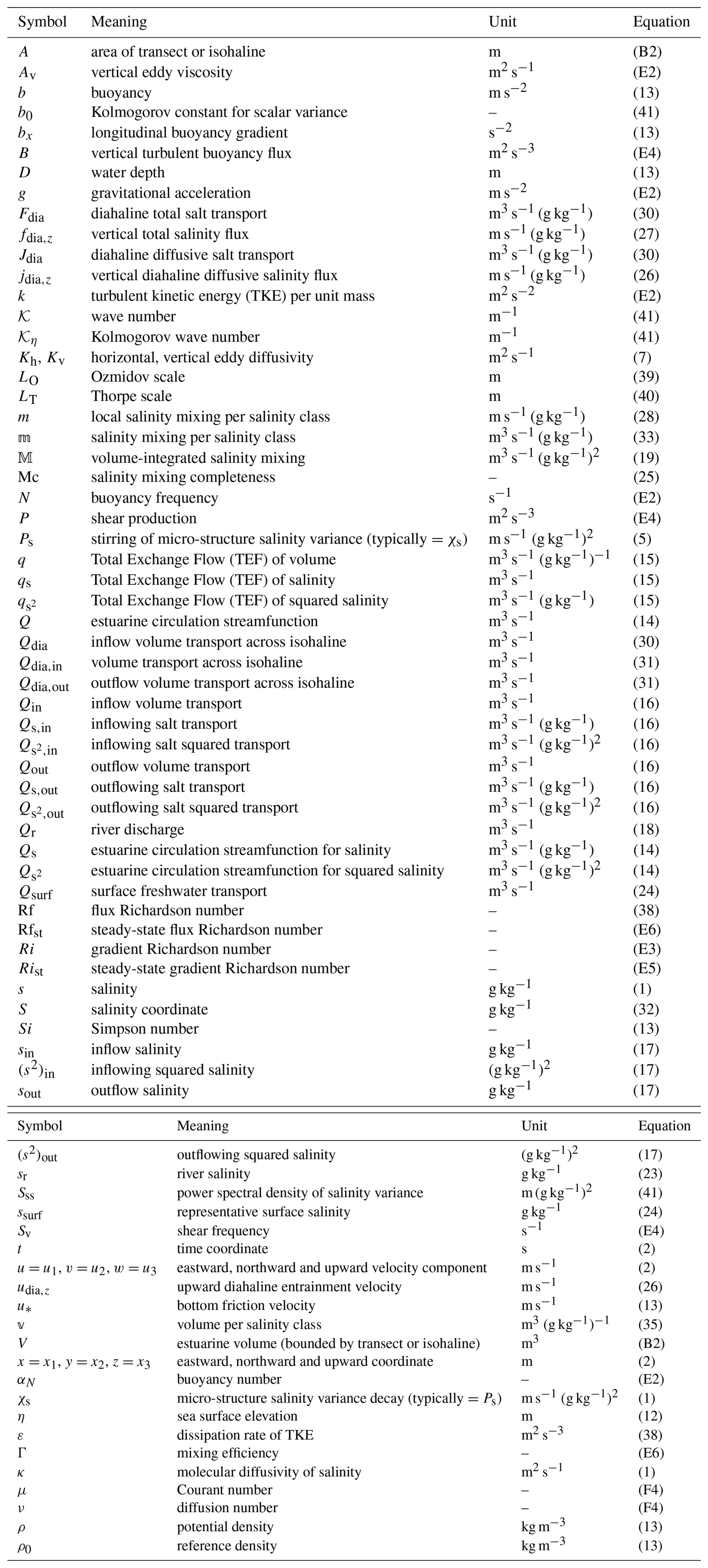
Table F2List of operators demonstrated for an arbitrary variable x.
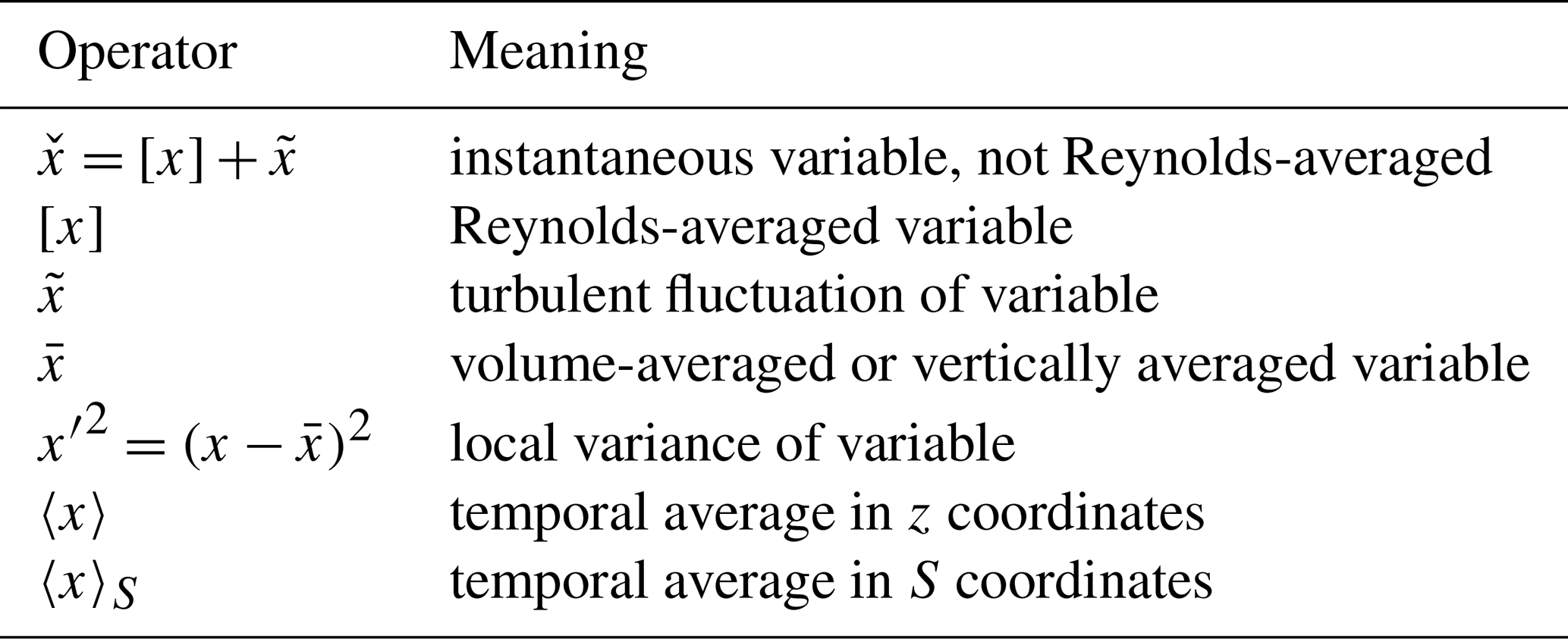
The used GETM source code is archived at https://doi.org/10.5281/zenodo.7741730 (Klingbeil, 2022).
The Elbe model data and the Python scripts used for the creation of the corresponding figures are archived at https://doi.org/10.5281/zenodo.20305994 (Li and Reese, 2026).
HB and WRG developed the first ideas, aims and structure for this review paper. HB wrote most of the text and designed the explanatory sketches. WRG wrote the Observations Sect. 5.1 and parts of the Introduction Sect. 1 and the Mixing processes Sect. 4. LR wrote the Appendix C on the Elbe River estuary simulations and KK wrote the derivation for the Coordinate transformation in Appendix D. Furthermore, KK checked all mathematical equations and derivations in detail. XL performed the Elbe River estuary model simulations for this review paper and LR and XL carried out the model analysis and the Elbe figures. WRG and KK implemented major changes to the structure of the manuscript. Finally, all authors reviewed, edited and corrected the entire manuscript in detail.
The contact author has declared that none of the authors has any competing interests.
Publisher's note: Copernicus Publications remains neutral with regard to jurisdictional claims made in the text, published maps, institutional affiliations, or any other geographical representation in this paper. The authors bear the ultimate responsibility for providing appropriate place names. Views expressed in the text are those of the authors and do not necessarily reflect the views of the publisher.
This article is part of the special issue “Ocean Science Jubilee: reviews and perspectives”. It is not associated with a conference.
The work of H. Burchard and K. Klingbeil is a contribution to the Collaborative Research Centre TRR 181 Energy Transfers in Atmosphere and Ocean (No. 274762653), funded by the German Research Foundation. We further acknowledge funding for X. Li by grant no. 03F0954F of the German Federal Ministry of Research, Technology and Space (BMFTR) as part of the DAM mission “mareXtreme”, project ElbeXtreme and for L. Reese by grant no. 03F0980B of the German Federal Ministry of Research, Technology and Space (BMFTR) as part of the DAM mission “sustainMare”, project CoastalFutures II. The authors are grateful for the useful comments and recommendations by Tobias Kukulka (University of Maryland, USA), Qing Li (The Hong Kong University of Science and Technology, Guangzhou, China) and Parker MacCready (University of Washington, USA). We further thank Robert Hetland (Pacific Northwest National Laboratory, USA), John Huthnance (National Oceanography Centre, UK) and an anonymous referee for their critical reviews of our original version of the manuscript.
This research has been supported by the Deutsche Forschungsgemeinschaft (grant no. TRR181) and the Bundesministerium für Forschung und Technologie (grant nos. 03F0980B and 03F0954F).
This paper was edited by John M. Huthnance and reviewed by Robert Hetland and one anonymous referee.
Armi, L. and Farmer, D. M.: Maximal two-layer exchange through a contraction with barotropic net flow, J. Fluid Mech., 164, 27–51, https://doi.org/10.1017/S0022112086002458, 1986. a
Banerjee, T., Klingbeil, K., and Danilov, S.: Discrete variance decay analysis of spurious mixing, Ocean Model., 192, 102460, https://doi.org/10.1016/j.ocemod.2024.102460, 2024. a, b
Becherer, J., Burchard, H., Flöser, G., Mohrholz, V., and Umlauf, L.: Evidence of tidal straining in well-mixed channel flow from micro-structure observations, Geophys. Res. Lett., 38, L17611, https://doi.org/10.1029/2011GL049005, 2011. a
Bo, T., Ralston, D. K., Garcia, A. M. P., and Geyer, W. R.: Tidal intrusion fronts, surface convergence, and mixing in an estuary with complex topography, J. Phys. Oceanogr., 54, 653–677, https://doi.org/10.1175/JPO-D-23-0131.1, 2024. a
Boehlich, M. J. and Strotmann, T.: The Elbe estuary, Die Küste, 74, 288–306, https://doi.org/10.18171/1.087106, 2008. a
Börgel, F., Karsten, S., Rummel, K., and Gräwe, U.: From weather data to river runoff: using spatiotemporal convolutional networks for discharge forecasting, Geosci. Model Dev., 18, 2005–2019, https://doi.org/10.5194/gmd-18-2005-2025, 2025. a
Boyle, E., Collier, R., Dengler, A., Edmond, J., Ng, A., and Stallard, R.: On the chemical mass-balance in estuaries, Geochim. Cosmochim. Ac., 38, 1719–1728, https://doi.org/10.1016/0016-7037(74)90188-4, 1974. a
Broatch, E. M. and MacCready, P.: Mixing in a salinity variance budget of the Salish Sea is controlled by river flow, J. Phys. Oceanogr., 52, 2305–2323, https://doi.org/10.1175/JPO-D-21-0227.1, 2022. a, b, c, d, e, f, g, h
Burchard, H.: A universal law of estuarine mixing, J. Phys. Oceanogr., 50, 81–93, https://doi.org/10.1175/JPO-D-19-0014.1, 2020. a, b, c, d, e, f, g
Burchard, H. and Bolding, K.: Comparative analysis of four second-moment turbulence closure models for the oceanic mixed layer, J. Phys. Oceanogr., 31, 1943–1968, https://doi.org/10.1175/1520-0485(2001)031<1943:caofsm>2.0.co;2, 2001. a, b, c, d
Burchard, H. and Bolding, K.: GETM – A General Estuarine Transport Model, Tech. Rep. EUR 20253 EN, European Commission, https://publications.jrc.ec.europa.eu/repository/handle/JRC23237 (last access: 16 June 2026), 2002. a
Burchard, H. and Hetland, R. D.: Quantifying the contributions of tidal straining and gravitational circulation to residual circulation in periodically stratified tidal estuaries, J. Phys. Oceanogr., 40, 1243–1262, https://doi.org/10.1175/2010JPO4270.1, 2010. a
Burchard, H. and Rennau, H.: Comparative quantification of physically and numerically induced mixing in ocean models, Ocean Model., 20, 293–311, https://doi.org/10.1016/j.ocemod.2007.10.003, 2008. a, b, c, d, e, f, g
Burchard, H., Bolding, K., and Villarreal, M. R.: GOTM – a general ocean turbulence model. Theory, applications and test cases, Tech. Rep. EUR 18745 EN, European Commission, https://op.europa.eu/en/publication-detail/-/publication/5b512e12-367d-11ea-ba6e-01aa75ed71a1 (last access: 16 June 2026), 1999. a
Burchard, H., Bolding, K., and Villarreal, M. R.: Three-dimensional modelling of estuarine turbidity maxima in a tidal estuary, Ocean Dyn., 54, 250–265, https://doi.org/10.1007/s10236-003-0073-4, 2004. a
Burchard, H., Hetland, R. D., Schulz, E., and Schuttelaars, H. M.: Drivers of residual estuarine circulation in tidally energetic estuaries: Straight and irrotational channels with parabolic cross section, J. Phys. Oceanogr., 41, 548–570, https://doi.org/10.1175/2010JPO4453.1, 2011. a, b
Burchard, H., Schulz, E., and Schuttelaars, H. M.: Impact of estuarine convergence on residual circulation in tidally energetic estuaries and inlets, Geophys. Res. Lett., 41, 913–919, https://doi.org/10.1002/2013GL058494, 2014. a
Burchard, H., Bolding, K., Feistel, R., Gräwe, U., Klingbeil, K., MacCready, P., Mohrholz, V., Umlauf, L., and van der Lee, E. M.: The Knudsen theorem and the Total Exchange Flow analysis framework applied to the Baltic Sea, Progr. Oceanogr., 165, 268–286, https://doi.org/10.1016/j.pocean.2018.04.004, 2018a. a, b, c, d, e, f, g
Burchard, H., Schuttelaars, H. M., and Ralston, D. K.: Sediment trapping in estuaries, Annu. Rev. Mar. Sci., 10, 10371–10395, https://doi.org/10.1146/annurev-marine-010816-060535, 2018b. a
Burchard, H., Lange, X., Klingbeil, K., and MacCready, P.: Mixing estimates for estuaries, J. Phys. Oceanogr., 49, 631–648, https://doi.org/10.1175/JPO-D-18-0147.1, 2019. a, b, c, d, e, f, g, h, i, j
Burchard, H., Gräwe, U., Klingbeil, K., Koganti, N., Lange, X., and Lorenz, M.: Effective diahaline diffusivities in estuaries, J. Adv. Model. Earth Sy., 13, https://doi.org/10.1029/2020MS002307, 2021. a, b
Burchard, H., Klingbeil, K., Lange, X., Li, X., Lorenz, M., MacCready, P., and Reese, L.: The relation between exchange flow and diahaline mixing in estuaries, J. Phys. Oceanogr., 55, 243–256, https://doi.org/10.1175/JPO-D-24-0105.1, 2025. a, b, c, d, e, f, g, h, i
Cessi, P.: The global overturning circulation, Annu. Rev. Mar. Sci., 11, 249–270, https://doi.org/10.1146/annurev-marine-010318-095241, 2019. a
Chang, Y., Li, X., Wang, Y. P., Klingbeil, K., Li, W., Zhang, F., and Burchard, H.: Salinity mixing in a tidal multi-branched estuary with huge and variable runoff, J. Hydrol., 634, 131094, https://doi.org/10.1016/j.jhydrol.2024.131094, 2024. a, b, c
Chen, S.-N. and Sanford, L. P.: Axial wind effects on stratification and longitudinal salt transport in an idealized, partially mixed estuary, J. Phys. Oceanogr., 39, 1905–1920, https://doi.org/10.1175/2009JPO4016.1, 2009. a
Chen, S.-N., Geyer, W. R., Ralston, D. K., and Lerczak, J. A.: Estuarine exchange flow quantified with isohaline coordinates: Contrasting long and short estuaries, J. Phys. Oceanogr., 42, 748–763, https://doi.org/10.1175/JPO-D-11-086.1, 2012. a, b, c, d, e, f
Cheng, Y., Canuto, V. M., and Howard, A. M.: An improved model for the turbulent PBL, J. Atmos. Sci., 59, 1550–1565, https://doi.org/10.1175/1520-0469(2002)059<1550:aimftt>2.0.co;2, 2002. a
Chrysagi, E., Umlauf, L., Holtermann, P., Klingbeil, K., and Burchard, H.: High-resolution simulations of submesoscale processes in the Baltic Sea: The role of storm events, J. Geophys. Res.-Oceans, 126, e2020JC016411, https://doi.org/10.1029/2020JC016411, 2021. a
Collignon, A. G. and Stacey, M. T.: Turbulence dynamics at the shoal–channel interface in a partially stratified estuary, J. Phys. Oceanogr., 43, 970–989, https://doi.org/10.1175/JPO-D-12-0115.1, 2013. a
Conroy, T., Sutherland, D. A., and Ralston, D. K.: Estuarine exchange flow variability in a seasonal, segmented estuary, J. Phys. Oceanogr., 50, 595–613, https://doi.org/10.1175/JPO-D-19-0108.1, 2020. a
Dijkstra, Y. M., Schuttelaars, H. M., and Burchard, H.: Generation of exchange flows in estuaries by tidal and gravitational eddy viscosity-shear covariance (ESCO), J. Geophys. Res.-Oceans, 122, 4217–4237, https://doi.org/10.1002/2016JC012379, 2017. a
Döös, K., Meier, H. M., and Döscher, R.: The Baltic haline conveyor belt or the overturning circulation and mixing in the Baltic, AMBIO, 33, 261–266, https://doi.org/10.1579/0044-7447-33.4.261, 2004. a, b
Drake, H. F., Shanice, B., Dussin, R., Griffies, S. M., Krasting, J. P., MacGilchrist, G. A., Stanley, G. J., Tesdal, J.-E., and Zika, J. D.: Water mass transformation budgets in finite-volume generalized vertical coordinate ocean models, J. Adv. Model. Earth Sy., 17, e2024MS004383, https://doi.org/10.1029/2024MS004383, 2025. a
Etemad-Shahidi, A. and Imberger, J.: Anatomy of turbulence in a narrow and strongly stratified estuary, J. Geophys. Res.-Oceans, 107, 7–1, https://doi.org/10.1029/2001JC000977, 2002. a
E.U. Copernicus Marine Service: Atlantic – European North West Shelf – Ocean Physics Analysis and Forecast, Marine Data Store (MDS) [data set], https://doi.org/10.48670/moi-00054, 2024. a
Ferrari, R., Mashayek, A., McDougall, T. J., Nikurashin, M., and Campin, J.-M.: Turning ocean mixing upside down, J. Phys. Oceanogr., 46, 2239–2261, https://doi.org/10.1175/JPO-D-15-0244.1, 2016. a
Fischer, H. B.: Mixing and dispersion in estuaries, Annu. Rev. Fluid Mech., 8, 107–133, https://doi.org/10.1146/annurev.fl.08.010176.000543, 1976. a
Galperin, B., Kantha, L., Rosati, A., and Hassid, S.: A quasi-equilibrium turbulent energy model for geophysical flows, J. Atmos. Sci., 45, 55–62, https://doi.org/10.1175/1520-0469(1988)045<0055:aqetem>2.0.co;2, 1988. a
Gargett, A. E.: Observing turbulence with a modified acoustic Doppler current profiler, J. Atmos. Ocean. Tech., 11, 1592–1610, https://doi.org/10.1175/1520-0426(1994)011<1592:otwama>2.0.co;2, 1994. a
Garrett, C.: Marginal mixing theories, Atmosphere-Ocean, 29, 313–339, https://doi.org/10.1080/07055900.1991.9649407, 1991. a
Garvine, R. W.: Penetration of buoyant coastal discharge onto the continental shelf: A numerical model experiment, J. Phys. Oceanogr., 29, 1892–1909, https://doi.org/10.1175/1520-0485(1999)029<1892:pobcdo>2.0.co;2, 1999. a, b
Geyer, W. R.: The importance of suppression of turbulence by stratification on the estuarine turbidity maximum, Estuaries, 16, 113–125, https://doi.org/10.2307/1352769, 1993. a
Geyer, W. R.: Influence of wind on dynamics and flushing of shallow estuaries, Estuar. Coast. Shelf S., 44, 713–722, https://doi.org/10.1006/ecss.1996.0140, 1997. a
Geyer, W. R. and MacCready, P.: The estuarine circulation, Annu. Rev. Fluid Mech., 46, 175–197, https://doi.org/10.1146/annurev-fluid-010313-141302, 2014. a, b
Geyer, W. R. and Ralston, D. K.: Estuarine frontogenesis, J. Phys. Oceanogr., 45, 546–561, https://doi.org/10.1175/JPO-D-14-0082.1, 2015. a, b, c
Geyer, W. R., Ralston, D. K., and Holleman, R. C.: Hydraulics and mixing in a laterally divergent channel of a highly stratified estuary, J. Geophys. Res.-Oceans, 122, 4743–4760, https://doi.org/10.1002/2016JC012455, 2017. a, b
Geyer, W. R., Ralston, D. K., and Chen, J.-L.: Mechanisms of exchange flow in an estuary with a narrow, deep channel and wide, shallow shoals, J. Geophys. Res., 125, e2020JC016092, https://doi.org/10.1029/2020JC016092, 2020. a
Gibbs, J. W.: On the equilibrium of heterogeneous substances, Am. J. Sci., 3, 441–458, https://doi.org/10.11588/heidok.00013220, 1878. a
Gibson, A. H., Hogg, A. M., Kiss, A. E., Shakespeare, C. J., and Adcroft, A. J.: Attribution of horizontal and vertical contributions to spurious mixing in an Arbitrary Lagrangian–Eulerian ocean model, Ocean Model., 119, 45–56, https://doi.org/10.1016/j.ocemod.2017.09.008, 2017. a
Giddings, S. N., Fong, D. A., and Monismith, S. G.: Role of straining and advection in the intratidal evolution of stratification, vertical mixing, and longitudinal dispersion of a shallow, macrotidal, salt wedge estuary, J. Geophys. Res.-Oceans, 116, https://doi.org/10.1029/2010JC006482, 2011. a, b
Gräwe, U., Holtermann, P., Klingbeil, K., and Burchard, H.: Advantages of vertically adaptive coordinates in numerical models of stratified shelf seas, Ocean Model., 92, 56–68, https://doi.org/10.1016/j.ocemod.2015.05.008, 2015. a
Gräwe, U., Flöser, G., Gerkema, T., Duran-Matute, M., Badewien, T. H., Schulz, E., and Burchard, H.: A numerical model for the entire Wadden Sea: Skill assessment and analysis of hydrodynamics, J. Geophys. Res., 121, 5231–5251, https://doi.org/10.1002/2016JC011655, 2016. a, b, c
Griffies, S. M.: Fundamentals of Ocean-Climate Models, Princeton University Press, Princeton, USA, ISBN 9780691118925, 2004. a
Griffies, S. M., Pacanowski, R. C., and Hallberg, R. W.: Spurious diapycnal mixing associated with advection in a z-coordinate ocean model, Mon. Weather Rev., 128, 538–564, https://doi.org/10.1175/1520-0493(2000)128<0538:sdmawa>2.0.co;2, 2000. a
Groeskamp, S., Griffies, S. M., Iudicone, D., Marsh, R., Nurser, A. G., and Zika, J. D.: The water mass transformation framework for ocean physics and biogeochemistry, Annu. Rev. Mar. Sci., 11, 271–305, https://doi.org/10.1146/annurev-marine-010318-095421, 2019. a, b
Harcourt, R. R.: An improved second-moment closure model of Langmuir turbulence, J. Phys. Oceanogr., 45, 84–103, https://doi.org/10.1175/JPO-D-14-0046.1, 2015. a
Henell, E., Burchard, H., Gräwe, U., and Klingbeil, K.: Spatial composition of the diahaline overturning circulation in a fjord-type, non-tidal estuarine system, J. Geophys. Res., 128, e2023JC019862, https://doi.org/10.1029/2023JC019862, 2023. a, b, c, d, e, f, g, h, i, j
Hetland, R.: Relating river plume structure to vertical mixing, J. Phys. Oceanogr., 35, 1667–1688, https://doi.org/10.1175/JPO2774.1, 2005. a, b
Hieronymus, M., Nilsson, J., and Nycander, J.: Water mass transformation in salinity–temperature space, J. Phys. Oceanogr., 44, 2547–2568, https://doi.org/10.1175/JPO-D-13-0257.1, 2014. a, b
Hofmeister, R., Beckers, J.-M., and Burchard, H.: Realistic modelling of the exceptional inflows into the central Baltic Sea in 2003 using terrain-following coordinates, Ocean Model., 39, 233–247, https://doi.org/10.1016/j.ocemod.2011.04.007, 2011. a, b
Holleman, R., Geyer, W., and Ralston, D.: Stratified turbulence and mixing efficiency in a salt wedge estuary, J. Phys. Oceanogr., 46, 1769–1783, https://doi.org/10.1175/JPO-D-15-0193.1, 2016. a, b, c, d, e, f
Holmes, R. M., Zika, J. D., Griffies, S. M., Hogg, A. M., Kiss, A. E., and England, M. H.: The geography of numerical mixing in a suite of global ocean models, J. Adv. Model. Earth Sy., 13, https://doi.org/10.1029/2020MS002333, 2021. a
Horner-Devine, A. R., Hetland, R. D., and MacDonald, D. G.: Mixing and transport in coastal river plumes, Annu. Rev. Fluid Mech., 47, 569–594, https://doi.org/10.1146/annurev-fluid-010313-141408, 2015. a
Huang, J., Chamecki, M., Li, Q., and Chen, B.: The role of longitudinal alignment between surface and bottom forcing on the full-column turbulence mixing in the coastal ocean, Ocean Model., 102637, https://doi.org/10.1016/j.ocemod.2025.102637, 2025. a
Huguenard, K., Valle-Levinson, A., Li, M., Chant, R., and Souza, A.: Linkage between lateral circulation and near-surface vertical mixing in a coastal plain estuary, J. Geophys. Res.-Oceans, 120, 4048–4067, https://doi.org/10.1002/2014JC010679, 2015. a
Huguenard, K., Bears, K., and Lieberthal, B.: Intermittency in Estuarine Turbulence: A framework toward limiting bias in microstructure measurements, J. Atmos. Ocean. Tech., 36, 1917–1932, https://doi.org/10.1175/JTECH-D-18-0220.1, 2019. a
Huzzey, L. M. and Brubaker, J. M.: The formation of longitudinal fronts in a coastal plain estuary, J. Geophys. Res.-Oceans, 93, 1329–1334, https://doi.org/10.1029/JC093iC02p01329, 1988. a
Ianniello, J. P.: Tidally induced residual currents in estuaries of variable breadth and depth, J. Phys. Oceanogr., 9, 962–974, https://doi.org/10.1175/1520-0485(1979)009<0962:TIRCIE>2.0.CO;2, 1979. a
Inall, M. and Gillibrand, P.: The physics of mid-latitude fjords: a review, in: Fjord Systems and Archives, edited by Howe, J. A., Austin, W. E. N., Forwick, M., and Paetzel, M., vol. 344 of Geological Society, London, Special Publications, The Geological Society of London London, 17–33, https://doi.org/10.1144/SP344.3, 2010. a
Jay, D. A. and Musiak, J. D.: Particle trapping in estuarine tidal flows, J. Geophys. Res., 99, 20445–20461, https://doi.org/10.1029/94JC00971, 1994. a
Ji, Z.-G., Hu, G., Shen, J., and Wan, Y.: Three-dimensional modeling of hydrodynamic processes in the St. Lucie Estuary, Estuar. Coast. Shelf S., 73, 188–200, https://doi.org/10.1016/j.ecss.2006.12.016, 2007. a
Kim, J., Park, K., Yang, D. R., and Hong, S.: A comprehensive review of energy consumption of seawater reverse osmosis desalination plants, Appl. Energ., 254, 113652, https://doi.org/10.1016/j.apenergy.2019.113652, 2019. a
Klingbeil, K.: Source code for the coastal ocean model GETM (tef branch), Zenodo [software], https://doi.org/10.5281/zenodo.7741730, 2022. a
Klingbeil, K. and Burchard, H.: Implementation of a direct nonhydrostatic pressure gradient discretisation into a layered ocean model, Ocean Model., 65, 64–77, https://doi.org/10.1016/j.ocemod.2013.02.002, 2013. a
Klingbeil, K. and Henell, E.: A rigorous derivation of the water mass transformation framework, the relation between mixing and diasurface exchange flow, and links to recent theories in estuarine research, J. Phys. Oceanogr., 53, 2953–2968, https://doi.org/10.1175/JPO-D-23-0130.1, 2023. a, b, c
Klingbeil, K. and Lorenz, M.: On the instantaneous salt mixing due to freshwater boundary fluxes, J. Phys. Oceanogr., 55, 809–813, https://doi.org/10.1175/JPO-D-24-0168.1, 2025. a
Klingbeil, K., Mohammadi-Aragh, M., Gräwe, U., and Burchard, H.: Quantification of spurious dissipation and mixing - Discrete variance decay in a Finite-Volume framework, Ocean Model., 81, 49–64, https://doi.org/10.1016/j.ocemod.2014.06.001, 2014. a, b, c
Klingbeil, K., Lemarié, F., Debreu, L., and Burchard, H.: The numerics of hydrostatic structured-grid coastal ocean models: State of the art and future perspectives, Ocean Model., 125, 80–105, https://doi.org/10.1016/j.ocemod.2018.01.007, 2018. a
Klingbeil, K., Becherer, J., Schulz, E., de Swart, H. E., Schuttelaars, H. M., Valle-Levinson, A., and Burchard, H.: Thickness-Weighted Averaging in tidal estuaries and the vertical distribution of the Eulerian residual transport, J. Phys. Oceanogr., 49, 1809–1826, https://doi.org/10.1175/JPO-D-18-0083.1, 2019. a
Knudsen, M.: Ein hydrographischer Lehrsatz, Annalen der Hydrographie und Maritimen Meteorologie, 28, 316–320, 1900. a, b, c, d, e, f, g, h, i
Kuhlbrodt, T., Griesel, A., Montoya, M., Levermann, A., Hofmann, M., and Rahmstorf, S.: On the driving processes of the Atlantic meridional overturning circulation, Rev. Geophys., 45, https://doi.org/10.1029/2004RG000166, 2007. a
Lange, X. and Burchard, H.: The relative importance of wind straining and gravitational forcing in driving exchange flows in tidally energetic estuaries, J. Phys. Oceanogr., 49, 723–736, https://doi.org/10.1175/JPO-D-18-0014.1, 2019. a
Lange, X., Klingbeil, K., and Burchard, H.: Inversions of estuarine circulation are frequent in a weakly tidal estuary with variable wind forcing and seaward salinity fluctuations, J. Geophys. Res.-Oceans, 125, e2019JC015789, https://doi.org/10.1029/2019JC015789, 2020. a, b
Lavery, A. C., Geyer, W. R., and Scully, M. E.: Broadband acoustic quantification of stratified turbulence, J. Acoust. Soc. Amer., 134, 40–54, https://doi.org/10.1121/1.4807780, 2013. a, b, c, d, e
Legay, A., Deremble, B., and Burchard, H.: Derivation and implementation of a non-local term to improve the oceanic convection representation within the k–ɛ parameterization, J. Adv. Model. Earth Sy., 17, e2024MS004243, https://doi.org/10.1029/2024MS004243, 2025. a, b
Lemagie, E., Giddings, S. N., MacCready, P., Seaton, C., and Wu, X.: Measuring estuarine total exchange flow from discrete observations, J. Geophys. Res.-Oceans, 127, e2022JC018960, https://doi.org/10.1029/2022JC018960, 2022. a, b, c
Lerczak, J. and Geyer, W.: Modeling the lateral circulation in straight, stratified estuaries, J. Phy. Oceanogr., 34, 1410–1428, https://doi.org/10.1175/1520-0485(2004)034<1410:MTLCIS>2.0.CO;2, 2004. a, b
Lesieur, M.: Turbulence in Fluids, Springer, https://doi.org/10.1007/978-1-4020-6435-7, 2008. a, b
Li, X. and Reese, L.: Dataset from Burchard et al. (2026): “Estuarine mixing”, Zenodo [data set], https://doi.org/10.5281/zenodo.20305994, 2026. a
Li, M., Trowbridge, J., and Geyer, W. R.: Asymmetric tidal mixing due to the horizontal density gradient, J. Phys. Oceanogr., 38, 418–434, https://doi.org/10.1175/2007JPO3372.1, 2008. a
Li, M., Radhakrishnan, S., Piomelli, U., and Geyer, W. R.: Large-eddy simulation of the tidal-cycle variations of an estuarine boundary layer, J. Geophys. Res.-Oceans, 115, https://doi.org/10.1029/2009JC005702, 2010. a
Li, Q., Bruggeman, J., Burchard, H., Klingbeil, K., Umlauf, L., and Bolding, K.: Integrating CVMix into GOTM (v6.0): a consistent framework for testing, comparing, and applying ocean mixing schemes, Geosci. Model Dev., 14, 4261–4282, https://doi.org/10.5194/gmd-14-4261-2021, 2021. a
Li, X., Geyer, W. R., Zhu, J., and Wu, H.: The transformation of salinity variance: A new approach to quantifying the influence of straining and mixing on estuarine stratification, J. Phys. Oceanogr., 48, 607–623, https://doi.org/10.1175/JPO-D-17-0189.1, 2018. a, b, c, d, e, f, g, h
Li, X., Lorenz, M., Klingbeil, K., Chrysagi, E., Gräwe, U., Wu, J., and Burchard, H.: Salinity mixing and diahaline exchange flow in a large multi-outlet estuary with islands, J. Phys. Oceanogr., 52, 2111–2127, https://doi.org/10.1175/JPO-D-21-0292.1, 2022. a, b, c, d, e, f, g
Li, X., Chrysagi, E., Klingbeil, K., and Burchard, H.: Impact of islands on tidally dominated river plumes: A high-resolution modeling study, J. Geophys. Res.-Oceans, 129, e2023JC020272, https://doi.org/10.1029/2023JC020272, 2024. a, b, c
Loder, T. C. and Reichard, R. P.: The dynamics of conservative mixing in estuaries, Estuaries, 4, 64–69, https://doi.org/10.2307/1351543, 1981. a
Lorenz, M., Klingbeil, K., MacCready, P., and Burchard, H.: Numerical issues of the Total Exchange Flow (TEF) analysis framework for quantifying estuarine circulation, Ocean Sci., 15, 601–614, https://doi.org/10.5194/os-15-601-2019, 2019. a, b
Lorenz, M., Klingbeil, K., and Burchard, H.: Numerical study of the exchange flow of the Persian Gulf using an extended total exchange flow analysis framework, J. Geophys. Res.-Oceans, 125, e2019JC015527, https://doi.org/10.1029/2019JC015527, 2020. a, b
Lorenz, M., Klingbeil, K., and Burchard, H.: Impact of evaporation and precipitation on estuarine mixing, J. Phys. Oceanogr., 51, 1319–1333, https://doi.org/10.1175/JPO-D-20-0158.1, 2021. a, b, c, d
Lu, Y. and Lueck, R. G.: Using a broadband ADCP in a tidal channel. Part II: Turbulence, J. Atmos. Ocean. Tech., 16, 1568–1579, https://doi.org/10.1175/1520-0426(1999)016<1568:UABAIA>2.0.CO;2, 1999. a
Lui, H.-K. and Chen, C.-T. A.: Shifts in limiting nutrients in an estuary caused by mixing and biological activity, Limnol. Oceanogr., 56, 989–998, https://doi.org/10.4319/lo.2011.56.3.0989, 2011. a
MacCready, P.: Toward a unified theory of tidally-averaged estuarine salinity structure, Estuaries, 27, 561–570, https://doi.org/10.1007/BF02907644, 2004. a
MacCready, P.: Calculating estuarine exchange flow using isohaline coordinates, J. Phys. Oceanogr., 41, 1116–1124, https://doi.org/10.1175/2011JPO4517.1, 2011. a, b, c, d, e, f
MacCready, P. and Banas, N.: Residual Circulation, Mixing, and Dispersion, in: Treatise on Estuarine and Coastal Science (Second Edition), edited by Baird, D. and Elliott, M., Academic Press, Oxford, 2nd Edn., 92–108, https://doi.org/10.1016/B978-0-323-90798-9.20006-1, 2011. a, b
MacCready, P. and Geyer, W. R.: Estuarine salt flux through an isohaline surface, J. Geophys. Res., 106, 11629–11637, https://doi.org/10.1029/2001JC900006, 2001. a
MacCready, P. and Geyer, W. R.: Advances in estuarine physics, Annu. Rev. Mar. Sci., 2, 35–58, https://doi.org/10.1146/annurev-marine-120308-081015, 2010. a, b, c, d
MacCready, P. and Geyer, W. R.: Estuarine exchange flow in the Salish Sea, J. Geophys. Res., 129, e2023JC020369, https://doi.org/10.1029/2023JC020369, 2024. a, b, c
MacCready, P., Hetland, R. D., and Geyer, W. R.: Long-term isohaline salt balance in an estuary, Cont. Shelf Res., 22, 1591–1601, https://doi.org/10.1016/S0278-4343(02)00023-7, 2002. a
MacCready, P., Geyer, W. R., and Burchard, H.: Estuarine exchange flow is related to mixing through the salinity variance budget, J. Phys. Oceanogr., 48, 1375–1384, https://doi.org/10.1175/JPO-D-17-0266.1, 2018. a, b, c, d, e, f, g, h, i, j, k, l
McPherson, R., Stevens, C., and O'Callaghan, J.: Turbulent scales observed in a river plume entering a fjord, J. Geophys. Res.-Oceans, 124, 9190–9208, https://doi.org/10.1029/2019JC015448, 2019. a
McWilliams, J. C.: Submesoscale currents in the ocean, Proc. R. Soc. Lond., A Math., 472, https://doi.org/10.1098/rspa.2016.0117, 2016. a
Mellor, G. L. and Yamada, T.: A hierarchy of turbulence closure models for planetary boundary layers, J. Atmos. Sci., 31, 1791–1806, https://doi.org/10.1175/1520-0469(1974)031<1791:AHOTCM>2.0.CO;2, 1974. a, b, c, d
Monismith, S. G., Burau, J. R., and Stacey, M.: Stratification dynamics and gravitational circulation in Northern San Francisco Bay, in: San Francisco Bay: the ecosystem, edited by Hollibaugh, J. T., American Association for the Advancement of Science, Pacific Division, San Francisco, 123–153, ISBN 9780934394116, 1996. a
Muche, Y., Klingbeil, K., Lorenz, M., Yankovsky, A. E., and Burchard, H.: Numerical investigation of the influence of wind and tides on salt mixing and cross-shore transport in river plumes, J. Geophys. Res.-Oceans, 131, e2025JC023583, https://doi.org/10.1029/2025JC023583, 2026. a
Munk, W. H.: Abyssal recipes, in: Deep sea research and oceanographic abstracts, Elsevier, vol. 13, 707–730, https://doi.org/10.1016/0011-7471(66)90602-4, 1966. a
Munk, W. H. and Wunsch, C.: Abyssal recipes II: Energetics of tidal and wind mixing, Deep-Sea Res. Pt. I, 45, 1977–2010, https://doi.org/10.1016/S0967-0637(98)00070-3, 1998. a
Nash, J. D. and Moum, J. N.: Microstructure estimates of turbulent salinity flux and the dissipation spectrum of salinity, J. Phys. Oceanogr., 32, 2312–2333, https://doi.org/10.1175/1520-0485(2002)032<2312:MEOTSF>2.0.CO;2, 2002. a, b
Nikurashin, M. and Ferrari, R.: Global energy conversion rate from geostrophic flows into internal lee waves in the deep ocean, Geophys. Res. Lett., 38, https://doi.org/10.1029/2011GL046576, 2011. a
Norwegian Meteorological Institute: MET Nordic operational archive, https://github.com/metno/NWPdocs/wiki/MET-Nordic-dataset (last access: 18 December 2024), 2024. a
Notz, D. and Worster, M. G.: Desalination processes of sea ice revisited, J. Geophys. Res.-Oceans, 114, https://doi.org/10.1029/2008JC004885, 2009. a
Nunes, R. and Simpson, J.: Axial convergence in a well-mixed estuary, Estuarine, Coast. Shelf Sci., 20, 637–649, https://doi.org/10.1016/0272-7714(85)90112-X, 1985. a
Osborn, T. R.: Estimates of the local rate of vertical diffusion from dissipation measurements, J. Phys. Oceanogr., 10, 83–89, https://doi.org/10.1175/1520-0485(1980)010<0083:EOTLRO>2.0.CO;2, 1980. a, b, c
Osborn, T. R. and Cox, C. S.: Oceanic fine structure, Geophys. Fluid Dyn., 3, 321–345, https://doi.org/10.1080/03091927208236085, 1972. a
Pemberton, P., Nilsson, J., Hieronymus, M., and Meier, H. M.: Arctic Ocean water mass transformation in S–T coordinates, J. Phys. Oceanogr., 45, 1025–1050, https://doi.org/10.1175/JPO-D-14-0197.1, 2015. a
Peters, H.: Observations of stratified turbulent mixing in an estuary: Neap-to-spring variations during high river flow, Estuar. Coast. Shelf S., 45, 69–88, https://doi.org/10.1006/ecss.1996.0180, 1997. a
Peters, H. and Bokhorst, R.: Microstructure observations of turbulent mixing in a partially mixed estuary. Part I: Dissipation rate, J. Phys. Oceanogr., 30, 1232–1244, https://doi.org/10.1175/1520-0485(2000)030<1232:MOOTMI>2.0.CO;2, 2000. a
Peters, H. and Bokhorst, R.: Microstructure observations of turbulent mixing in a partially mixed estuary. Part II: Salt flux and stress, J. Phys. Oceanogr., 31, 1105–1119, https://doi.org/10.1175/1520-0485(2001)031<1105:MOOTMI>2.0.CO;2, 2001. a, b, c
Pietrzak, J. D.: The use of TVD limiters for forward-in-time upstream-biased advection schemes in ocean modeling, Mon. Weather Rev., 126, 812–830, https://doi.org/10.1175/1520-0493(1998)126<0812:TUOTLF>2.0.CO;2, 1998. a
Pritchard, D. W.: Observations of circulation in coastal plain estuaries, Estuaries, AAAS Publ., 83, 37–44, 1967. a
Purkiani, K., Becherer, J., Flöser, G., Gräwe, U., Mohrholz, V., Schuttelaars, H. M., and Burchard, H.: Numerical analysis of stratification and destratification processes in a tidally energetic inlet with an ebb tidal delta, J. Geophys. Res.-Oceans, 120, 225–243, https://doi.org/10.1002/2014JC010325, 2015. a
Qu, L., Hetland, R. D., and Schlichting, D.: Mixing pathways in simple box models, J. Phys. Oceanogr., 52, 2761–2772, https://doi.org/10.1175/JPO-D-22-0074.1, 2022. a
Ralston, D. K., Cowles, G. W., Geyer, W. R., and Holleman, R. C.: Turbulent and numerical mixing in a salt wedge estuary: Dependence on grid resolution, bottom roughness, and turbulence closure, J. Geophys. Res., 122, 692–712, https://doi.org/10.1002/2016JC011738, 2017. a, b, c
Ramadhan, A., Wagner, G., Hill, C., Campin, J.-M., Churavy, V., Besard, T., Souza, A., Edelman, A., Ferrari, R., and Marshall, J.: Oceananigans. jl: Fast and friendly geophysical fluid dynamics on GPUs, J. Open Source Software, 5, https://doi.org/10.21105/joss.02018, 2020. a
Rayson, M. D., Gross, E. S., Hetland, R. D., and Fringer, O. B.: Using an isohaline flux analysis to predict the salt content in an unsteady estuary, J. Phys. Oceanogr., 47, 2811–2828, https://doi.org/10.1175/JPO-D-16-0134.1, 2017. a
Reese, L., Gräwe, U., Klingbeil, K., Li, X., Lorenz, M., and Burchard, H.: Local mixing determines spatial structure of diahaline exchange flow in a mesotidal estuary: A study of extreme runoff conditions, J. Phys. Oceanogr., 54, 3–27, https://doi.org/10.1175/JPO-D-23-0052.1, 2024. a, b, c, d, e, f, g, h, i, j, k, l, m, n, o
Reese, L., Becker, M., Holtermann, P., Li, X., and Burchard, H.: The role of the shoal – salt mixing mechanisms in a partially mixed tidal estuary with channel-shoal geometry, Cont. Shelf Res., 299, 105669, https://doi.org/10.1016/j.csr.2026.105669, 2026. a, b, c, d, e, f, g
Rippeth, T. P., Fisher, N., and Simpson, J. H.: The cycle of turbulent dissipation in the presence of tidal straining, J. Phys. Oceanogr., 31, 2458–2471, https://doi.org/10.1175/1520-0485(2001)031<2458:TCOTDI>2.0.CO;2, 2001. a
Rodi, W.: Examples of calculation methods for flow and mixing in stratified fluids, J. Geophys. Res., 92, 5305–5328, https://doi.org/10.1029/JC092iC05p05305, 1987. a, b
Ross, L., Huguenard, K., and Sottolichio, A.: Intratidal and fortnightly variability of vertical mixing in a macrotidal estuary: The Gironde, J. Geophys. Res.-Oceans, 124, 2641–2659, https://doi.org/10.1029/2018JC014456, 2019. a
Rummel, K., Strauß, T., Lauer, F., and Gräwe, U.: Real-time prediction of salt intrusion in tidal estuaries using long short-term memory networks, J. Geophys. Res.-Mach., 2, e2025JH000768, https://doi.org/10.1029/2025JH000768, 2025. a, b
Schlichting, D., Qu, L., Kobashi, D., and Hetland, R.: Quantification of physical and numerical mixing in a coastal ocean model using salinity variance budgets, J. Adv. Model. Earth Sy., 15, e2022MS003380, https://doi.org/10.1029/2022MS003380, 2023. a, b
Schumann, U. and Gerz, T.: Turbulent mixing in stably stratified shear flows, J. Appl. Meteorol., 34, 33–48, 1995. a
Scully, M. E. and Friedrichs, C. T.: Sediment pumping by tidal asymmetry in a partially mixed estuary, J. Geophys. Res.-Oceans, 112, https://doi.org/10.1029/2006JC003784, 2007. a
Scully, M. E., Friedrichs, C. T., and Brubaker, J.: Control of estuarine stratification and mixing by wind-induced straining of the estuarine density field, Estuaries, 28, 321–326, https://doi.org/10.1007/BF02693915, 2005. a, b
Scully, M. E., Michel, A. P., Nicholson, D. P., and Traylor, S.: Spatial and temporal variations in atmospheric gas flux from the Hudson River: the estuarine gas exchange maximum, Limnol. Oceanogr., 67, 1590–1603, https://doi.org/10.1002/lno.12154, 2022. a
Shchepetkin, A. F. and McWilliams, J. C.: The regional oceanic modelling system (ROMS): a split-explicit, free-surface, topography-following-coordinate oceanic model, Ocean Model., 9, 347–404, https://doi.org/10.1016/j.ocemod.2004.08.002, 2005. a
Simpson, J. H., Brown, J., Matthews, J., and Allen, G.: Tidal straining, density currents, and stirring in the control of estuarine stratification, Estuar. Coast., 13, 125–132, https://doi.org/10.2307/1351581, 1990. a, b, c, d, e, f
Skyllingstad, E. D. and Wijesekera, H. W.: Large-eddy simulation of flow over two-dimensional obstacles: high drag states and mixing, J. Phys. Oceanogr., 34, 94–112, https://doi.org/10.1175/1520-0485(2004)034<0094:LSOFOT>2.0.CO;2, 2004. a
Smagorinsky, J.: General circulation experiments with the primitive equations: I. The basic experiment, Mon. Weather Rev., 91, 99–164, https://doi.org/10.1175/1520-0493(1963)091<0099:GCEWTP>2.3.CO;2, 1963.
Smolarkiewicz, P. K.: Multidimensional positive definite advection transport algorithm: an overview, Int. J. Num. Meth. Fluids, 50, 1123–1144, https://doi.org/10.1002/fld.1071, 2006. a
Stacey, M. T., Fram, J. P., and Chow, F. K.: Role of tidally periodic density stratification in the creation of estuarine subtidal circulation, J. Geophys. Res., 113, C08016, https://doi.org/10.1029/2007JC004581, 2008. a
Stacey, M. W., Monismith, S. G., and Burau, J. R.: Measurements of Reynolds stress profiles in unstratified tidal flow, J. Geophys. Res., 104, 10933–10949, https://doi.org/10.1029/1998JC900095, 1999. a
Strotmann, T.: Deutsches Gewässerkundliches Jahrbuch. Elbegebiet, Teil III. Untere Elbe ab der Havelmündung 2014, ISSN 0949-3654, 2017. a
Sutherland, D. A., MacCready, P., Banas, N. S., and Smedstad, L. F.: A model study of the Salish Sea estuarine circulation, J. Phys. Oceanogr., 41, 1125–1143, https://doi.org/10.1175/2011JPO4540.1, 2011. a, b, c, d, e
Thorpe, S. A.: Turbulence and mixing in a Scottish loch, Phil. Trans. R. Soc. Lond. A 286, 125–181, https://doi.org/10.1098/rsta.1977.0112, 1977. a
Trowbridge, J., Geyer, W., Bowen, M., and Williams III, A.: Near-bottom turbulence measurements in a partially mixed estuary: Turbulent energy balance, velocity structure, and along-channel momentum balance, J. Phys. Oceanogr., 29, 3056–3072, https://doi.org/10.1175/1520-0485(1999)029<3056:NBTMIA>2.0.CO;2, 1999. a
Umlauf, L.: A note on the description of mixing in stratified layers without shear in large-scale ocean models, J. Phys. Oceanogr., 39, 3032–3039, https://doi.org/10.1175/2009JPO4006.1, 2009. a
Umlauf, L. and Burchard, H.: A generic length-scale equation for geophysical turbulence models, J. Mar. Res., 61, 235–265, 2003. a
Umlauf, L. and Burchard, H.: Second-order turbulence models for geophysical boundary layers. A review of recent work, Cont. Shelf Res., 25, 795–827, https://doi.org/10.1016/j.csr.2004.08.004, 2005. a, b, c, d, e, f
Verspecht, F. I., Burchard, H., Rippeth, T. P., Howarth, M. J., and Simpson, J. H.: Processes impacting on stratification in a region of freshwater influence: Application to Liverpool Bay, J. Geophys. Res.-Oceans, 114, 11022, https://doi.org/10.1029/2009JC005475, 2009. a
Walin, G.: A theoretical framework for the description of estuaries, Tellus, 29, 128–136, https://doi.org/10.3402/tellusa.v29i2.11337, 1977. a, b, c, d, e, f, g, h, i, j, k, l, m
Walin, G.: On the relation between sea-surface heat flow and thermal circulation in the ocean, Tellus, 34, 187–195, https://doi.org/10.1111/j.2153-3490.1982.tb01806.x, 1982. a
Wang, T. and Geyer, W. R.: The balance of salinity variance in a partially stratified estuary: Implications for exchange flow, mixing, and stratification, J. Phys. Oceanogr., 48, 2887–2899, https://doi.org/10.1175/JPO-D-18-0032.1, 2018. a, b
Wang, T., Geyer, W. R., and MacCready, P.: Total exchange flow, entrainment, and diffusive salt flux in estuaries, J. Phys. Oceanogr., 47, 1205–1220, https://doi.org/10.1175/JPO-D-16-0258.1, 2017. a, b, c, d, e, f, g, h, i, j
Wang, X., Kukulka, T., and Plueddemann, A. J.: Wind fetch and direction effects on Langmuir turbulence in a coastal ocean, J. Geophys. Res.-Oceans, 127, e2021JC018222, https://doi.org/10.1029/2021JC018222, 2022. a
Warner, J. C., Geyer, W. R., and Lerczak, J. A.: Numerical modeling of an estuary: A comprehensive skill assessment, J. Geophys. Res.-Oceans, 110, https://doi.org/10.1029/2004JC002691, 2005a. a, b
Warner, J. C., Sherwood, C. R., Arango, H. G., and Signell, R. P.: Performance of four turbulence closure models implemented using a generic length scale method, Ocean Model., 8, 81–113, https://doi.org/10.1016/j.ocemod.2003.12.003, 2005b. a
Warner, J. C., Geyer, W. R., Ralston, D. K., and Kalra, T.: Using tracer variance decay to quantify variability of salinity mixing in the Hudson River estuary, J. Geophys. Res., 125, e2020JC016096, https://doi.org/10.1029/2020JC016096, 2020. a, b, c, d, e, f, g
Wasserstraßen- und Schifffahrtsamt Magdeburg: Abflussstation Neu Darchau, https://www.kuestendaten.de/DE/Services/Messreihen_Dateien_Download/Download_Zeitreihen_node.html (last access: 18 December 2024), 2024. a
Xiong, J., Shen, J., and Qin, Q.: Exchange flow and material transport along the salinity gradient of a long estuary, J. Geophys. Res.-Oceans, 126, e2021JC017185, https://doi.org/10.1029/2021JC017185, 2021. a
Yan, C., McWilliams, J. C., and Chamecki, M.: Overlapping boundary layers in coastal oceans, J. Phys. Oceanogr., 52, 627–646, https://doi.org/10.1175/JPO-D-21-0067.1, 2022. a
Yin, D., Ralston, D. K., Warner, J. C., Ganju, N. K., and Harris, C. K.: Wind pumping dominates landward salt transport in a weakly tidal estuary, J. Geophys. Res.-Oceans, 130, e2025JC022683, https://doi.org/10.1029/2025JC022683, 2025. a
Yu, L.: On sea surface salinity skin effect induced by evaporation and implications for remote sensing of ocean salinity, J. Phys. Oceanogr., 40, 85–102, https://doi.org/10.1175/2009JPO4168.1, 2010. a
Zalesak, S. T.: Fully multidimensional flux-corrected transport algorithms for fluids, J. Comput. Phys., 31, 335–362, https://doi.org/10.1016/0021-9991(79)90051-2, 1979. a
Zhang, Y. J., Ye, F., Stanev, E. V., and Grashorn, S.: Seamless cross-scale modeling with SCHISM, Ocean Model., 102, 64–81, https://doi.org/10.1016/j.ocemod.2016.05.002, 2016. a
- Abstract
- Introduction
- Quantification of mixing
- Estuarine circulation and mixing
- Major mixing processes and estuarine mixing hotspots
- Methods to quantify mixing
- Future Perspectives
- Appendix A: Stirring and mixing: the case of saltwater in a glass beaker
- Appendix B: Salinity-variance equations
- Appendix C: Elbe River estuary model
- Appendix D: Coordinate transformation of vertical salinity equation
- Appendix E: Calibration of two-equation turbulence closure models
- Appendix F: Derivations for numerical mixing example
- Code availability
- Data availability
- Author contributions
- Competing interests
- Disclaimer
- Special issue statement
- Acknowledgements
- Financial support
- Review statement
- References