Regional modeling of internal-tide dynamics around New Caledonia – Part 1: Coherent internal-tide characteristics and sea surface height signature

The southwestern tropical Pacific exhibits a complex bathymetry and represents a hot spot of internal-tide generation. Based on a tailored high-resolution regional model, we investigate for the first time the internal-tide field around the New Caledonia islands through energy budgets that quantify the coherent internal-tide generation, propagation, and dissipation. A total of 15.27 GW is converted from the barotropic to the baroclinic M2 tide with the main conversion sites associated with the most prominent bathymetric structures such as continental slopes and narrow passages in the north (2.17 GW) and ridges and seamounts south of New Caledonia (3.92 GW). The bulk of baroclinic energy is generated in shallow waters around 500 m depth and on critical to supercritical slopes, highlighting the limitations of linear semi-analytical models in those areas. Despite the strongly dominant mode-1 generation, more than 50 % of the locally generated energy either dissipates in the near field close to the generation sites or loses coherence. The remaining baroclinic energy propagates within well-defined tidal beams with baroclinic energy fluxes of up to 30 kW m⁻¹ toward the open ocean. The New Caledonia site represents a challenge for SWOT (Surface Water and Ocean Topography) observability of balanced motion in the presence of internal tides with sea surface height (SSH) signatures >6 cm at similar wavelengths. We show for our study region that a correction of SSH for the coherent internal tide potentially increases the observability of balanced motion from wavelengths >160 km to well below 100 km.

1 Introduction

The flow of barotropic tidal oceanic currents over bathymetry such as continental slopes, ridges, and seamounts represents a major source of baroclinic energy in the global ocean in the form of internal tides (i.e., internal waves at tidal frequency) expressed by high-frequency fluctuations and vertical displacements of isopycnal surfaces (Bell, 1975; Smith and Young, 2002; Garrett and Kunze, 2007). From a global point of view, internal tides have received increasing attention in recent decades as they provide a route to energy dissipation away from lateral boundaries and the surface through diapycnal mixing with important implications for open-ocean mixing and the global oceanic energy budget (e.g., Munk and Wunsch, 1998; Melet et al., 2013; Waterhouse et al., 2014; Kunze, 2017a, b).

Internal tides express themselves in vertical oscillations of density surfaces with strong baroclinic velocities. They are characterized by a complex vertical structure that can be described by a discrete set of vertical normal modes via the Sturm–Liouville problem (Gill, 1982; Arbic et al., 2018; Buijsman et al., 2020). Low vertical modes have large horizontal wavelengths (𝒪(150 km)), usually form over large-scale topographic features, and propagate over large distances (𝒪(1000 km); Dushaw et al., 1995; St. Laurent and Garrett, 2002; Alford, 2003; Zhao et al., 2010, 2016). In contrast, high vertical modes feature smaller horizontal wavelengths that are generated over smaller-scale topographic features. They tend to dissipate locally not far away from the formation sites due to their lower group velocities and higher vertical shear (Zhao et al., 2016; Vic et al., 2019). Characterizing internal tides, their vertical structure, and propagation is thus key to better understanding their contribution to mixing.

Yet, it is still challenging through both observations and model experiments. Some scattered in situ observations with high-frequency sampling, such as moorings, can help to characterize these processes at some locations (e.g., Zilberman et al., 2011; Vic et al., 2018), but they do not provide a global view. Alternatively, altimetric sea surface height (SSH) observations have been extensively used to globally estimate the SSH imprint of internal tides by using, e.g., empirical models that are based on an up to 20-year-long record of conventional altimeter missions (Zhao et al., 2016; Ray and Zaron, 2016; Zaron, 2019; Ubelmann et al., 2022). These estimates have provided us with a robust representation of the coherent internal tide, which is defined here as a phase-locked internal tide constant in amplitude and phase that is determined over a long time series. However, satellite altimetry generally provides very limited information about internal-tide vertical structure, allowing the detection of the first and second vertical modes only.

The characterization of internal tides with their vertical modes (each associated with a different wavelength) and their signature in SSH is an important task for the Surface Water and Ocean Topography (SWOT) satellite mission (launched in December 2022). SWOT is expected to provide new insights into small-scale ocean dynamics by resolving wavelengths at up to 10 times higher resolution (down to 15 km; Fu et al., 2012; Fu and Ubelmann, 2014) than conventional altimetry (𝒪100 km; Ballarotta et al., 2019) with SSH imprints from mesoscale and submesoscale dynamics down to high-frequency internal wave motion, as well as the interaction between them (Fu and Ferrari, 2008; Morrow et al., 2019). From an oceanographic point of view, the characterization of the mesoscale and submesoscale circulation is the primary objective of SWOT (Morrow et al., 2019). The challenge lies in disentangling the measured SSH signal associated with balanced and unbalanced motions, i.e., eddies and gravity waves, since they can feature similar spatial scales. This highlights the need for a detailed picture of internal-tide dynamics to properly derive mesoscale and submesoscale motions (Zaron, 2019; Carrere et al., 2021). Numerical modeling has been playing an important role in partly overcoming the constraints of in situ observations and altimetry. Dedicated studies of internal-tide characteristics and energetics near internal-tide generation hot spots have been conducted in various regions such as the Hawaiian Ridge (Carter et al., 2008), Luzon Strait (Kerry et al., 2013), Solomon Sea (Tchilibou et al., 2020), Amazonian Shelf (Tchilibou et al., 2022), and Mid-Atlantic Ridge (Lahaye et al., 2020). The energy converted from barotropic to baroclinic tides, the distribution of the vertical modes generated, the local ratio between dissipation and conversion, and the energy propagation all heavily depend on the local bathymetric features and the background state, emphasizing the need for a regional focus with high-resolution regional simulations.

Here, we provide the first comprehensive description of the internal-tide field around New Caledonia in the southwestern tropical Pacific using the output of a tailored high-resolution regional simulation from a full-model calendar year (Fig. 1). This region has not received much attention despite being known as an internal-tide generation hot spot from numerical modeling of internal tides in early stages (Niwa and Hibiya, 2001). It is characterized by complex bathymetry of large-scale ridges, very steep slopes, shelf breaks, basins, and seamounts at mid-depths and in the near surface that give rise to propagating tidal beams over several hundred kilometers and significant signatures in SSH as deduced from satellite altimetry (Ray and Zaron, 2016).

New Caledonia also represents an interesting site to study eddy–internal-tide interactions due to a complex regional circulation (Qu and Lindstrom, 2002; Kessler and Cravatte, 2013; Cravatte et al., 2015). Through the interaction with the background currents, the internal-tide field around New Caledonia is potentially subject to temporal variability, also referred to as tidal incoherence in the literature (e.g., Dunphy and Lamb, 2014; Dunphy et al., 2017; Ponte et al., 2017; Lamb and Dunphy, 2018; Shakespeare and Hogg, 2019). An additional reason to study the internal tides around New Caledonia is their potential role in the marine biodiversity for which the region is internationally recognized (Payri et al., 2019). This is especially true south of New Caledonia where seamounts and ridges are hot spots of biodiversity providing marine habitats for marine mammals, fish, and small-scale organisms (Payri and de Forges, 2006; Ganachaud et al., 2010; Gardes et al., 2014; Menkès et al., 2015). Internal tides may also have important implications for coastal ecosystems, mitigating heat stress (Wyatt et al., 2020, 2023) or enhancing upwelling of nutrient-rich waters to the surface (Wolanski and Pickard, 1985; Leichter et al., 2003).

Lastly, the region is crossed by the SWOT swaths during SWOT's fast sampling phase (1 d repeat orbit, Fig. 1a). In this context, New Caledonia serves as a calibration and validation (CalVal) site within the SWOT program and the associated Adopt-A-Crossover (AdAC) consortium. A dedicated field campaign was carried out in spring 2023 to collect high-frequency measurements of the governing fine-scale physics. It thus represents a unique opportunity to address SSH observability of mesoscale and submesoscale dynamics, internal tides, and their interaction.

Due to the study's extent, this work is subject to a series of two papers. Part 1 focuses on stationary, coherent internal tides, whereas Part 2 focuses on nonstationary, incoherent internal tides addressing mesoscale activity as a source of this incoherence.

This study's overall objective for Part 1 is twofold: (1) a detailed introduction to the regional modeling effort that has been explicitly designed to shed light on the internal-tide dynamics around New Caledonia in the framework of SWOT–AdAC, including a model assessment; (2) a detailed description of the coherent internal-tide energetics providing a first picture of the local dynamics at work. Here, we will address the following scientific questions. What areas around New Caledonia are subject to internal-tide generation and dissipation? What is the internal tide's modal content? How is the internal tide expressed in SSH, and at which wavelengths are we able to observe mesoscale and submesoscale processes?

The study is organized as follows. In Sect. 2, we introduce the high-resolution modeling strategy, the tidal analyses and diagnostics used in this study, and the different datasets or products used to assess our simulation. The model assessment is presented in Sect. 3, where we estimate the model ability to realistically simulate the mean circulation, the mesoscale activity, and the barotropic tides. In Sect. 4, we quantify the energetics of the dominant internal tide in the region around New Caledonia and in the hot spots of internal-tide generation. Internal-tide SSH signature is investigated in Sect. 5 in the context of SWOT observability. We finish with a summary and discussion in Sect. 6.

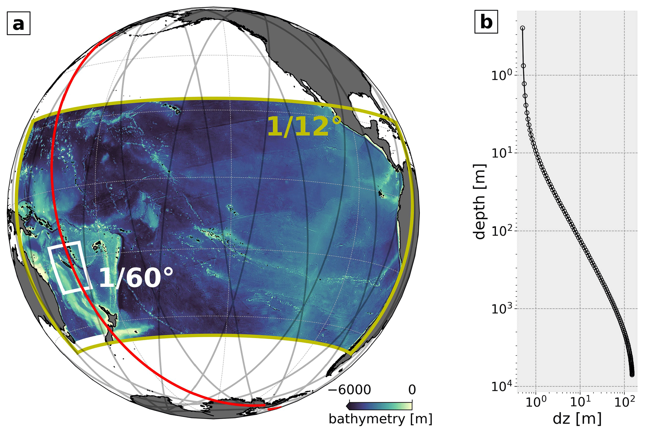
Figure 1 (a) Model setup showing the host grid domain (TROPICO12, yellow box) and the nesting grid (CALEDO60, white box) including the bathymetry (shading) and the SWOT CalVal orbit (black transparent lines) with the highlighted ground track (red line) that crosses the CALEDO60 domain. (b) TROPICO12 and CALEDO60 vertical resolution among 125 vertical levels.

2 Data and methods

2.1 Model setup

The model used in this study is based on the Nucleus for European Model.ing of the Ocean (NEMO, code version 4.0.6, Madec and Team, 2023), which solves the three-dimensional primitive equations on a staggered Arakawa-C-type grid. The model grid consists of a host grid (TROPICO12) at $\mathrm{1}/\mathrm{12}{}^{\circ }$ horizontal resolution that spans the Pacific Ocean basin from 142–290^∘ E and 24^∘ N–46^∘ S (Fig. 1a). The ridge features 125 vertical levels with 0.5 m thickness at the surface increasing toward 150 m in the deep ocean with 75 vertical levels in the upper 1000 m (Fig. 1b). In the vertical, the model uses a partial-step z coordinate with a nonlinear free surface.

Further, the model setup features a horizontal grid refinement (nesting), named CALEDO60, at $\mathrm{1}/{\mathrm{60}}^{\circ }$ horizontal resolution (∼1.7 km grid box spacing). In this particular region, it is expected to allow the model to be submesoscale-permitting. The nesting grid is located in the southwestern tropical Pacific from 159.2–172.4^∘ E and 15.7–28.8^∘ S and encompasses New Caledonia (see Fig. 1a). The nesting was set up using an Adaptive Grid Refinement In Fortran (AGRIF, Debreu et al., 2008), a tool explicitly designed for NEMO to set up regional simulations embedded in a pre-defined configuration. AGRIF enables the two-way lateral boundary coupling between the host and the nesting grid to be integrated sequentially during the whole length of the simulation.

Laplacian isopycnal diffusion coefficients for tracers were chosen to be mesh-size-dependent such that the tracer diffusion is scaled down from the host grid of 93 m² s⁻¹ to the nesting grid of 4 m² s⁻¹. Vertical eddy diffusivity is estimated by a turbulent kinetic energy (TKE) closure scheme (Gaspar et al., 1990). It is based on a prognostic equation for turbulent kinetic energy and a closure assumption for turbulent length scales depending on vertical shear, stratification, vertical diffusion, and dissipation. The advection of momentum is parameterized by means of a third-order scheme based on upstream-biased parabolic interpolation (UBS).

Initial conditions for temperature and salinity for TROPICO12 and CALEDO60 are prescribed by the GLORYS2V4 oceanic reanalysis (https://doi.org/10.48670/moi-00023). Atmospheric forcing is taken from ERA5 produced by the European Centre for Medium-Range Weather Forecasts (ECMWF, Hersbach et al., 2020) provided at hourly temporal resolution and a spatial resolution of $\mathrm{1}/{\mathrm{4}}^{\circ }$ to compute surface fluxes using bulk formulae and the prognostic sea surface temperature from the model. Wind stress is computed following the methodology from Renault et al. (2016), i.e., wind speed minus surface currents.

Both domains are forced by the tidal potential of the five major tidal constituents (M2, S2, N2, K1, O1). TROPICO12 is forced at its open lateral boundaries with daily currents, temperature, and salinity, likewise using GLORYS2V4. In addition, TROPICO12 is forced at the open lateral boundaries by SSH and barotropic currents of the same five tidal constituents taken from the global tide atlas FES2014 (Finite Element Solution 2014, Lyard et al., 2021). We made this limited choice to allow the separation of these constituents at monthly timescales.

Recent studies have highlighted the importance of taking into account remote forcing of high-frequency oceanic variability for regional simulations, as it may represent a non-negligible source of energy (Jeon et al., 2019; Nelson et al., 2020; Mazloff et al., 2020; Siyanbola et al., 2023). Further, it was suggested that tidal accuracy and predictability increase when implementing a two-way nesting framework between the high-resolution regional domain and the lower-resolution host grid (Jeon et al., 2019). The authors show that mass and energy are conserved with no evident discontinuities along the nesting boundaries.

Apart from increasing predictability through higher horizontal resolution of the nesting grid, it is argued that a realistic bathymetry product is also essential. For the CALEDO60 domain, we used a specific bathymetric product based on the GEBCO_2019 grid (GEBCO, 2019) and a compilation of multibeam echosounder data acquired over the years in the New Caledonia economic zone (Roger et al., 2021). The latter product, initially at 200 m resolution, only covers the area 155^∘ E–175.1^∘ N, 14.1–26.6^∘ S. It has been combined with the GEBCO_2019 bathymetry product to cover the full domain.

Internal tides represent a large source of diapycnal mixing in the open ocean. The associated parameterization scheme developed by St. Laurent et al. (2002) is usually used in NEMO simulations. Here, it has been turned off because our simulation has a resolution large enough to resolve the internal wave dynamics. In fact, it has been recently suggested that turning off background components of the vertical mixing scheme improves the modeled kinetic energy levels (Thakur et al., 2022).

The bottom friction is parameterized using a logarithmic boundary layer with a drag coefficient of $\mathrm{3}\times {\mathrm{10}}^{-\mathrm{3}}$ (maximum value of 0.1), a roughness of $\mathrm{2.5}\times {\mathrm{10}}^{-\mathrm{3}}$ m, and a background kinetic energy of $\mathrm{1}\times {\mathrm{10}}^{-\mathrm{2}}$ m² s⁻². These values yielded the best visual agreement with respect to the mean regional circulation, i.e., the location and magnitude of zonal jets.

The model has been spun up for 2 years (model years 2012–2013) before being run for a total of 5 years (model years 2014–2018). Here, if not noted otherwise, we only focus on 2014 (neutral El Niño–Southern Oscillation conditions) with instantaneous fields saved hourly for the three-dimensional temperature, salinity, velocity, and surface fields (including SSH) for CALEDO60. For TROPICO12, the instantaneous three-dimensional variables are given at daily resolution, whereas the surface fields are saved at hourly resolution. A twin experiment with identical forcing and parameterization has been initialized, but without barotropic tide forcing. Being subject to a future study, here, it is only used to compare the energy spectrum with the tidal simulation.

2.2 Tidal analysis and diagnostics

2.2.1 Tidal harmonics

In order to investigate the tidal dynamics at play in the regional CALEDO60 simulation, we first apply a harmonic analysis to a full-model calendar year time series (model year 2014) of the three-dimensional velocity and pressure fields to extract the semi-diurnal (M2, S2, N2) and diurnal (K1, O1) tidal constituents. The choice of a full-model calendar year relies upon a compromise between high computational expenses and the representative extraction of the coherent tide through a time series long enough to isolate seasonal and mesoscale variability. Therefore and if not noted otherwise, we define the coherent internal tide as a phase-locked internal tide with constant amplitude and phase referenced to the full-model calendar year time series.

2.2.2 Barotropic–baroclinic modal decomposition

The study of internal tides requires an accurate separation of the barotropic and baroclinic tides. The barotropic tide is directly linked to the astronomical tide forcing. In contrast to baroclinic tides, it is independent of depth and density stratification (Hendershott, 1981, see  Sect. 1). Several approaches to separate barotropic and baroclinic tides have been discussed in detail, for example in Kelly et al. (2010), Nugroho (2017), and Tchilibou et al. (2020). Here, we use a vertical-mode decomposition approach by solving the Sturm–Liouville problem obeying a linear free surface while assuming a flat bottom:

$$\begin{array}{}\text{(1)}& {\displaystyle }& {\displaystyle \frac{{\partial }^{\mathrm{2}}{\mathrm{\Phi }}_n}{\partial z^{\mathrm{2}}}}+{\displaystyle \frac{N^{\mathrm{2}}}{c_n^{\mathrm{2}}}}{\mathrm{\Phi }}_n=\mathrm{0},\text{(2)}& {\displaystyle }& {\displaystyle }{\mathrm{\Phi }}_n={\displaystyle \frac{c_n^{\mathrm{2}}}{g}}{\displaystyle \frac{\partial {\mathrm{\Phi }}_n}{\partial z}}\text{at}z=\mathrm{0},\text{and}\text{(3)}& {\displaystyle }& {\displaystyle }{\mathrm{\Phi }}_n=\mathrm{0}\text{at}z=-H,\end{array}$$

with the given buoyancy frequency N defined as

$$\begin{array}{}\text{(4)}& N^{\mathrm{2}}=-{\displaystyle \frac{g}{{\mathit{\rho }}_{\mathrm{0}}}}{\displaystyle \frac{\partial \mathit{\rho }}{\partial z}},\end{array}$$

where ρ is the potential density, z the vertical coordinate, g the gravitational acceleration, and ρ₀ the reference density. c_n is the eigenspeed and Φ_n the eigenfunction describing the vertical structure for vertical velocity and displacement (McDougall and Barker, 2011). It is related to the eigenfunction describing the vertical structure for horizontal velocity and pressure via

$$\begin{array}{}\text{(5)}& {\mathit{\varphi }}_n={\mathit{\rho }}_{\mathrm{0}}{c}_n^{\mathrm{2}}{\displaystyle \frac{\partial {\mathrm{\Phi }}_n}{\partial z}}.\end{array}$$

In practice, the Sturm–Liouville eigenvalue problem has been solved at each grid point of the model, using the annual mean density field referenced to the same period as the harmonic analysis above, for the 10 lowest modes, where the lowest mode (n=0) refers to the barotropic tide and n≥1 represents the baroclinic modes. Based on the tidal harmonics determined in Sect. 2.2.1, the model variables are projected onto the orthogonal, discrete set of normal vertical modes, i.e.,

$$\begin{array}{}\text{(6)}& \begin{array}{rl}& \left[\mathit{u}\right(x,y,z,t),p(x,y,z,t\left)\right]\\ & =\sum _{n=\mathrm{0}}^{\mathrm{9}}\left[{\mathit{u}}_n\right(x,y,t),p_n(x,y,t\left)\right]{\mathit{\varphi }}_n\left(z\right),\end{array}\end{array}$$

for the horizontal velocity vector $\mathit{u}=(u,v)$ and pressure p, as well as

$$\begin{array}{}\text{(7)}& w(x,y,z,t)=\sum _{n=\mathrm{0}}^{\mathrm{9}}{w}_n(x,y,t){\mathrm{\Phi }}_n\left(z\right),\end{array}$$

for the vertical velocity w using a least squares fit method. If not specified otherwise, we define the baroclinic tide as the sum of modes 1–9. As will be seen in Sect. 4, this is sufficient in our study region, where low baroclinic modes are strongly dominant.

2.2.3 Energy equations

The redistribution and transfer of energy from the barotropic tide to the internal tide can be approximated by the barotropic and baroclinic energy equation neglecting the tendency term and nonlinear advection following Simmons et al. (2004), Carter et al. (2008), and Buijsman et al. (2014, 2017) since both terms were found to be at least 1 order of magnitude smaller:

$$\begin{array}{}\text{(8)}& {\displaystyle }& {\displaystyle }{\mathbf{\nabla }}_{\text{h}}\cdot {\mathit{F}}_{\text{bt}}+D_{\text{bt}}+C=\mathrm{0},\text{(9)}& {\displaystyle }& {\displaystyle }{\mathbf{\nabla }}_{\text{h}}\cdot {\mathit{F}}_{\text{bc}}+D_{\text{bc}}-C=\mathrm{0},\end{array}$$

where ∇_h⋅F is the energy flux divergence with ${\mathbf{\nabla }}_{\text{h}}=(\partial /\partial x,\partial /\partial y)$ the horizontal gradient operator and $\mathit{F}=(F_x,F_y)$ the energy flux vector, D is the energy dissipation, and C is the barotropic-to-baroclinic conversion term. The subscripts bt and bc stand for the barotropic and baroclinic tide. In the barotropic energy equation, the conversion is considered a sink of energy, whereas it is an energy source in the baroclinic energy equation. The conversion term is defined as

$$\begin{array}{}\text{(10)}& C={\mathbf{\nabla }}_{\text{h}}H\langle \mathit{u}{p}_{\text{bc}}(-H)\rangle ,\end{array}$$

where H is the bathymetry, $\mathit{u}=(u_{\text{bt}},v_{\text{bt}})$ the barotropic tidal velocity vector, and p_bc the baroclinic tidal pressure at the ocean bottom (−H). 〈〉 denotes the average over a tidal cycle. Following Zilberman et al. (2009), we compute 〈u_bt p_bc(−H)〉 via

$$\begin{array}{}\text{(11)}& \langle {\mathit{u}}_{\text{bt}}{p}_{\text{bc}}(-H)\rangle ={\displaystyle \frac{\mathrm{1}}{\mathrm{2}}}{A}_{p_{\text{bc}}(-H)}{A}_{\mathit{u}}\cos ({\mathit{\phi }}_{p_{\text{bc}}(-H)}-{\mathit{\phi }}_{\mathit{u}}),\end{array}$$

where A and φ are the respective amplitude and phase of the tidal harmonic obtained from p_bc and u_bt. The conversion for each mode n is given by

$$\begin{array}{}\text{(12)}& C^n={\mathbf{\nabla }}_{\text{h}}H\langle {\mathit{u}}_{\text{bt}}{p}_{\text{bc}}^n(-H)\rangle ,\end{array}$$

where $p_{\text{bc}}^n(-H)$ is the baroclinic pressure at the ocean bottom (−H) for mode n. Equivalent to Eq. (11), we compute for each mode n:

$$\begin{array}{}\text{(13)}& \langle {\mathit{u}}_{\text{bt}}{p}_{\text{bc}}^n(-H)\rangle ={\displaystyle \frac{\mathrm{1}}{\mathrm{2}}}{A}_{p_{\text{bc}}^n(-H)}{A}_{{\mathit{u}}_{\text{bt}}}\cos ({\mathit{\phi }}_{p_{\text{bc}}^n(-H)}-{\mathit{\phi }}_{{\mathit{u}}_{\text{bt}}}).\end{array}$$

The propagation of barotropic and baroclinic tide energy is expressed by the energy flux (F_bt and F_bc) and is considered here to be a depth-integrated quantity:

$$\begin{array}{}\text{(14)}& {\displaystyle }& {\displaystyle }{\mathit{F}}_{\text{bt}}=\underset{-H}{\overset{\mathit{\eta }}{\int }}\langle {\mathit{u}}_{\text{bt}}{p}_{\text{bt}}\rangle \mathrm{d}z,\text{(15)}& {\displaystyle }& {\displaystyle }{\mathit{F}}_{\text{bc}}=\underset{-H}{\overset{\mathit{\eta }}{\int }}\langle {\mathit{u}}_{\text{bc}}{p}_{\text{bc}}\rangle \mathrm{d}z,\end{array}$$

where p_bt is the barotropic pressure, and ${\mathit{u}}_{\text{bc}}=(u_{\text{bc}},v_{\text{bc}})$ is the baroclinic velocity vector. The baroclinic energy flux for each mode n is defined as

$$\begin{array}{}\text{(16)}& {\displaystyle }{\mathit{F}}_{\text{bc}}^n=\underset{-H}{\overset{\mathit{\eta }}{\int }}\langle {\mathit{u}}_{\text{bc}}^n{p}_{\text{bc}}^n\rangle \mathrm{d}z,\end{array}$$

where ${\mathit{u}}_{\text{bc}}^n$ is the baroclinic tidal velocity vector for mode n. Note that the average over a tidal cycle follows the same methodology as for the conversion term above. The barotropic (D_bt) and baroclinic (D_bc) dissipation is regarded as the residual of the energy flux divergence and conversion and is, hence, obtained through Eqs. (8) and (9), respectively. As will be discussed later, D_bc may contain both true baroclinic energy dissipation and scattering to the incoherent tide.

In the following, we mainly focus our study on the M2 semi-diurnal tide, which explains in the nesting domain more than 80 % of the total energy conversion from the barotropic to the baroclinic tide while representing about 84 % of the semi-diurnal energy conversion (see Table 1).

Table 1 Full CALEDO60 domain, area-integrated barotropic-to-baroclinic conversion in gigawatts (GW) for each tidal constituent (M2, S2, N2, K1, O1) with their respective contribution to the total in percent.

2.3 Other data

2.3.1 CARS climatology and merged Argo–CARS velocity product

The model used in this study is evaluated using climatology and observations. Model stratification and water mass vertical structure are evaluated using climatological hydrography data taken from the CSIRO Atlas of Regional Seas (CARS2009) that provides gridded maps of temperature and salinity by combining a variety of datasets (Ridgway et al., 2002, http://www.marine.csiro.au/~dunn/cars2009/, last access 21 February 2021). The large-scale regional mean circulation in the Coral Sea is compared to the Argo–CARS merged velocity product from Kessler and Cravatte (2013). This product derives absolute geostrophic currents using climatological hydrographic data from CARS2009 referenced to a level of known motion of 1000 m obtained by drifting trajectories of Argo floats.

2.3.2 Altimetry-derived EKE

Surface mesoscale eddy kinetic energy (EKE) during the period 2014–2018 is evaluated using global ocean gridded maps ($\mathrm{1}/{\mathrm{4}}^{\circ }$) of SSH generated and processed by the EU Copernicus Marine Environment Monitoring Service (CMEMS, https://doi.org/10.48670/moi-00148). In detail, we use the multimission Data Unification and Altimeter Combination System (DUACS) product in delayed time and daily resolution with all satellite missions available at a given time. Mesoscale EKE was derived from the geostrophic velocity field as follows:

$$\begin{array}{}\text{(17)}& \text{EKE}={\displaystyle \frac{\mathrm{1}}{\mathrm{2}}}\stackrel{\mathrm{‾}}{u_g^{\prime \mathrm{2}}+v_g^{\prime \mathrm{2}}},\end{array}$$

where $u_g=-\frac{g}{f}\frac{\partial \mathit{\eta }}{\mathrm{d}y}$, $v_g=\frac{g}{f}\frac{\partial \mathit{\eta }}{\mathrm{d}x}$ with f the Coriolis parameter and η the SSH above geoid (also referred to as absolute dynamic topography), and $(u_g^{\prime },v_g^{\prime })=(u_g-\stackrel{\mathrm{‾}}{u_g},v_g-\stackrel{\mathrm{‾}}{v_g})$ where the overbar denotes the temporal average over the period 2014–2018. Additionally, the geostrophic velocities were high-pass-filtered at a cut-off period of 180 d to account for the mesoscale (Qiu and Chen, 2004). We computed the modeled EKE as closely as possible to the altimetric EKE.

2.3.3 In situ mooring

As part of an assessment of the SARAL/ALtiKa satellite altimeter for the monitoring of the East Caledonian Current flowing along Loyalty Ridge, moorings and gliders have been deployed along the satellite ground track (Durand et al., 2017). Here, we take advantage of the current meter mooring at 167.26^∘ E, 20.44^∘ S (about 30 km off the northern tip of Lifou island in the core of the ECC; see Fig. 2a). The mooring was deployed from November 2010 to October 2011 at the bottom of the continental slope in 3300 m water depth. It was equipped with an upward-looking LinkQuest FlowQuest 300 kHz acoustic Doppler current profiler (ADCP; with 4 m bins) located at a mean depth of 80 m and five RCM7 Aanderaa rotor current meters at 300, 400, 500, 600, and 1000 m. The mooring provided hourly records of the 1 min averaged ocean velocity over the upper 1000 m. Here, it is used to compare in situ kinetic energy with the model (see Sect. 3.3)

2.3.4 FES2014

The FES2014 global ocean tidal atlas (Lyard et al., 2021) is the latest release to improve tidal predictions based on the hydrodynamic modeling of tides (Toulouse Unstructured Grid Ocean model, further denoted T-UGOm) coupled to an ensemble data assimilation code (spectral ensemble optimal interpolation, denoted SpEnOI). It is a very significant upgrade compared to the previous atlases, thanks to the improvement of the assimilated data accuracy and the model performance. FES2014 has been integrated in satellite altimetry geophysical data records (GDRs). It also provides very accurate open-boundary tidal conditions for regional and coastal modeling. Here, it is used to ensure the correct representation of the barotropic tide for SSH in both the host and nesting grid.

2.3.5 HRET

The expression of internal tides in SSH in our model simulation is evaluated by the High Resolution Empirical Tide version 8.1 (HRET8.1, https://ingria.ceoas.oregonstate.edu/~zarone/downloads.html, last access 12 September 2022, Zaron, 2019; Carrere et al., 2021). The product uses essentially all exact-repeat altimeter mission data in the period 1992–2017 (TOPEX/Jason, GEOSAT, ERS, Envisat). In contrast to other previous approaches, HRET differs by the subtraction of the mesoscale sea level anomaly from the SSH along the ground tracks. This ensures having as little non-tidal variability as possible. This is followed by a harmonic analysis applied to a time series at each point along the ground track for missions with the same orbit.

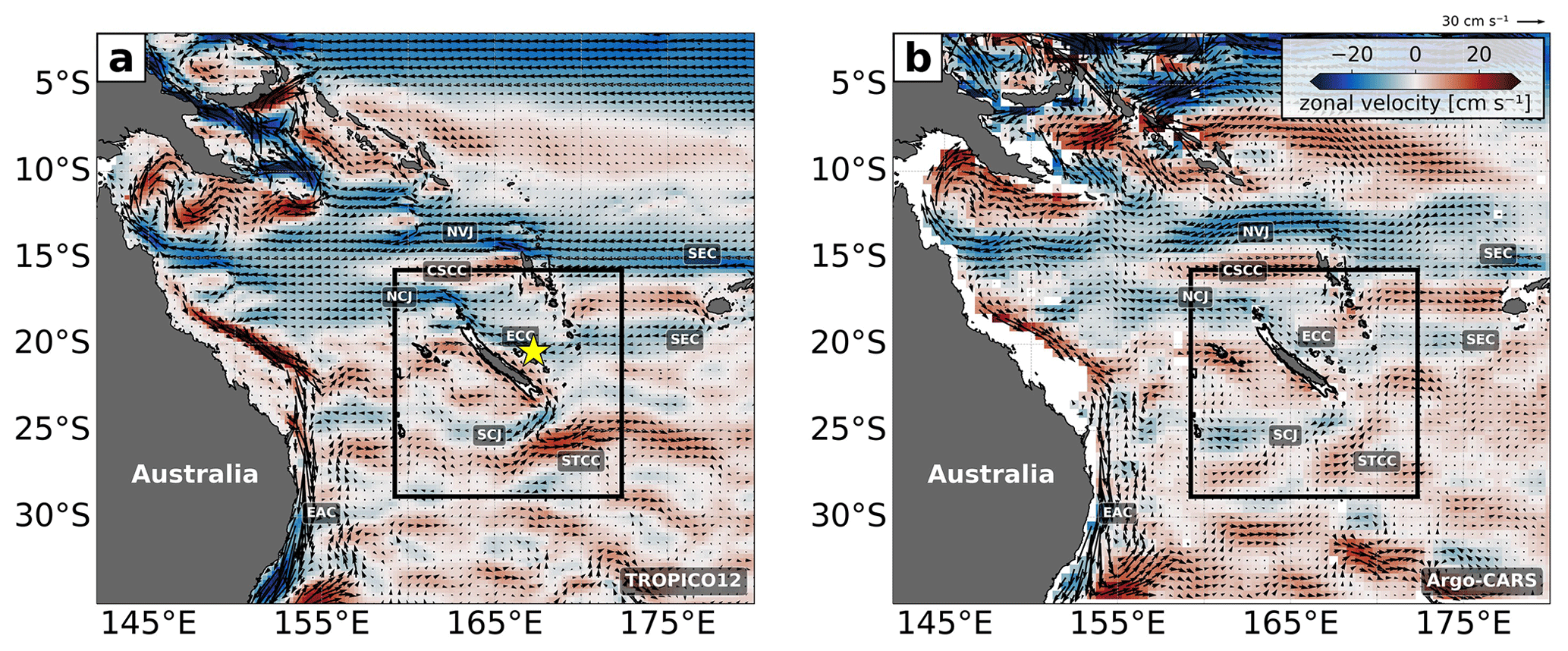
Figure 2 Coral Sea near-surface (20–100 m) regional circulation illustrating zonal velocity (shading) and velocity vectors from (a) TROPICO12 (2014–2018 mean) and (b) the Argo–CARS merged velocity product (Kessler and Cravatte, 2013). The black box indicates the CALEDO60 domain. The major currents are labeled: South Equatorial Current (SEC), North Vanuatu Jet (NVJ), Coral Sea Countercurrent (CSCC), North Caledonian Jet (NCJ), East Caledonian Current (ECC), South Caledonian Jet (SCJ), Subtropical Countercurrent (STCC), and East Australian Current (EAC). The location of the in situ mooring (see Sect. 2.3.3) is indicated by the yellow star.

2.3.6 Semi-analytical models of tidal energy conversion

Semi-analytical models have been developed to obtain a global estimate of energy conversion rates from the barotropic to the baroclinic tide using bottom topography, climatological stratification, and tidal barotropic velocity (e.g., Nycander, 2005; Falahat et al., 2014; Vic et al., 2019). Doing so, they are highly valuable for tidal mixing parameterizations in ocean and climate models that do not have the ability to explicitly resolve tidal processes (MacKinnon et al., 2017; de Lavergne et al., 2019, 2020). Here, we make use of the products from Falahat et al. (2014) and Vic et al. (2019) to evaluate our model energy conversion. At the same time, we emphasize the limited capability of semi-analytical models to accurately predict internal-tide generation in shallow waters and in areas of complex bathymetry such as New Caledonia. Specifically, semi-analytical models break down for bathymetric slopes that are equal to or larger than the internal-tide wave slopes, i.e., critical to supercritical slopes. The wave ray-path slope s is obtained from the dispersion relation as follows:

$$\begin{array}{}\text{(18)}& s=\sqrt{{\displaystyle \frac{{\mathit{\omega }}^{\mathrm{2}}-f^{\mathrm{2}}}{N^{\mathrm{2}}-{\mathit{\omega }}^{\mathrm{2}}}}},\end{array}$$

where ω is the tidal frequency. The buoyancy frequency N is taken from near the ocean bottom. The steepness parameter α, defined as the ratio of the seafloor topographic slope to the ray-path slope, qualifies the seafloor topography as subcritical (α<0.8 s), critical (0.8 s $\le \mathit{\alpha }\le \mathrm{1.5}$ s), and supercritical (α>1.5 s), following de Lavergne et al. (2019). Semi-analytical models are often corrected for energy conversion in the shallow waters due to violation of linear theory. Initially corrected for the upper 400 m in Falahat et al. (2014) and the upper 700 m in Vic et al. (2019), we also correct Falahat et al. (2014) for the upper 700 m to ensure the best comparison between the two products.

3 Model assessment

In the following, we will assess the model's capability to realistically reproduce motion from the large-scale circulation down to high-frequency motion while justifying the model's eligibility to simulate internal-tide dynamics.

3.1 Mean circulation

The modelization of the regional circulation in the Coral Sea represents a challenge due to the numerous islands that serve as obstacles, forming boundary currents and westward jets as well as recirculation and eastward countercurrents (Couvelard et al., 2008; Qiu et al., 2009). The main feature is a westward inflow from the South Pacific subtropical gyre, which splits into strong zonal jets, western boundary currents, and eastward countercurrents when encountering bathymetric features (Couvelard, 2007; Kessler and Cravatte, 2013; Cravatte et al., 2015; Qiu and Chen, 2004). The 2014–2018 mean near-surface (20–100 m) simulated velocity field (Fig. 2a) is compared to the Argo–CARS merged velocity (see Sect. 2.3.1 for a description, Fig. 2b). The model 5-year mean shows good agreement with the observed regional circulation. The westward zonal jets are well represented with the South Equatorial Current (SEC) being split into the North Vanuatu Jet (NVJ) and the North Caledonian Jet (NCJ) north of New Caledonia and the South Caledonian Jet (SCJ) south of New Caledonia. West of the main islands (New Caledonia, Vanuatu, Fiji), the observed surface eastward countercurrents are also well simulated (Qiu et al., 2009). The circulation south of New Caledonia seems more variable, with less clearly defined mean currents in both products. There is evidence of the presence of the surface-intensified eastward Subtropical Countercurrent (STCC) that emerges from the East Australian Current (EAC) recirculation (Ridgway and Dunn, 2003). It is clearly intensified in the model, but the Argo merged product south of New Caledonia should be taken with caution since limited observations do not average out the signatures of ubiquitous mesoscale eddies. Overall, the mean circulation is well simulated, which is essential for the proper description of eddy–internal-tide interactions that are the subject of Part 2 of this study.

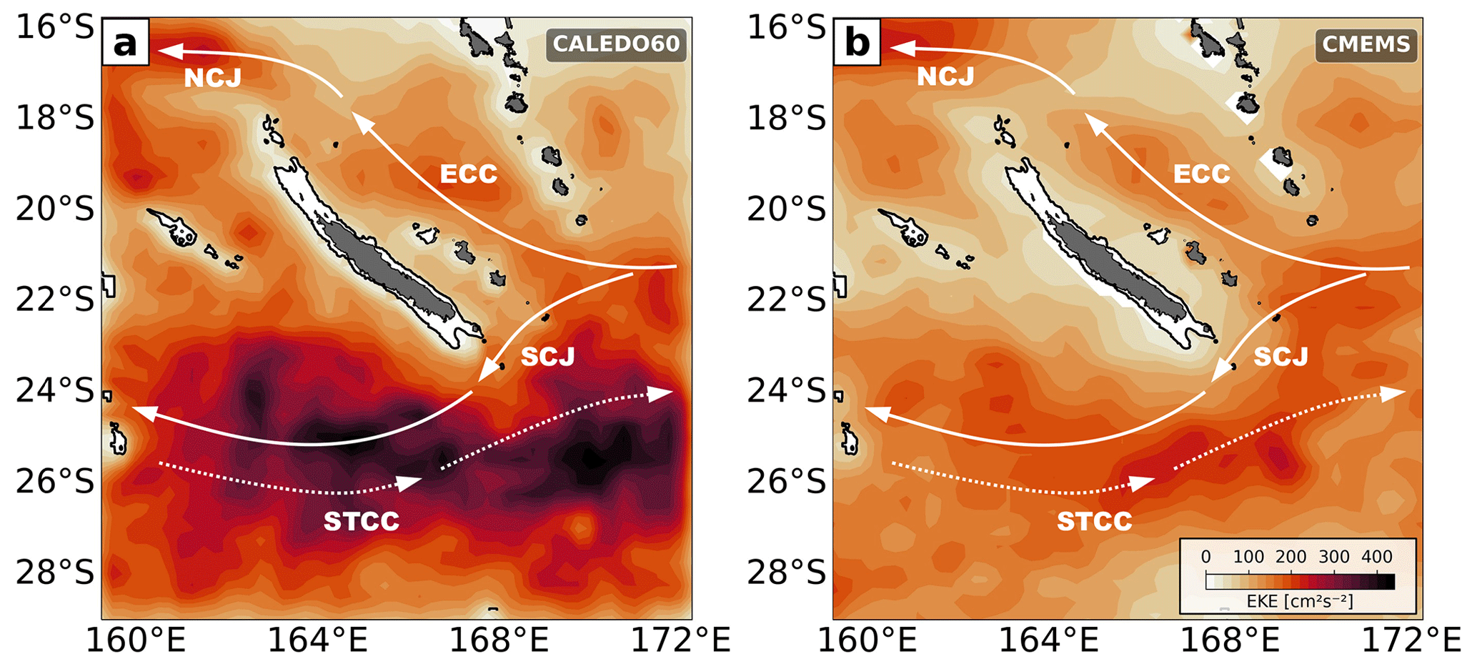
Figure 3 Surface mesoscale EKE derived from SSH for (a) CALEDO60 and (b) CMEMS altimeter products and averaged for the period 2014–2018. Currents are labeled as in Fig. 2.

3.2 Mesoscale variability

The large-scale circulation around New Caledonia is subject to barotropic and baroclinic instability of horizontally and vertically sheared currents (Qiu and Chen, 2004; Qiu et al., 2008, 2009) giving rise to mesoscale eddy variability. Here, the spatial pattern of the surface model mesoscale EKE (Fig. 3a) is compared to the mesoscale EKE as observed by satellite altimetry (Fig. 3b). We computed the modeled EKE as closely as possible to the altimetric EKE. To do so, we computed the 5 d mean of the model SSH to eliminate high-frequency variability such as tidal and inertial motions before horizontally binning the data onto the grid of present-day altimetry ($\mathrm{1}/{\mathrm{4}}^{\circ }$). For proper comparison between model and altimeter observations, we also computed the 5 d average for altimetric SSH before the derivation of mesoscale EKE. Mesoscale EKE is maximum south of New Caledonia where mesoscale activity is expected to be generated through baroclinic instabilities of the vertically sheared SEC and SCJ–STCC (Qiu et al., 2009; Keppler et al., 2018). Elevated levels of EKE are also found along the eastern boundary current system between New Caledonia and Vanuatu as well as in the northwest of the domain through horizontal shear between the westward NCJ and the eastward Coral Sea Countercurrent (Figs. 2, 3a). The spatial pattern of simulated EKE is in good agreement with satellite altimetry (Fig. 3b). Maximum levels of EKE in the southern domain where mesoscale activity is high are essentially lower than in the model (>250 cm² s⁻² compared to >400 cm² s⁻²). We argue that this can be attributed to the present-day two-dimensional gridded satellite altimetry products. They are derived by gridding and optimal interpolation of available along-track SSH data, projected onto a $\mathrm{1}/{\mathrm{4}}^{\circ }$ horizontal grid, and do not resolve wavelengths smaller than 150–200 km in our study region (Ballarotta et al., 2019). The model, even though gridded to $\mathrm{1}/{\mathrm{4}}^{\circ }$ resolution, might contain dynamics that are associated with smaller scales.

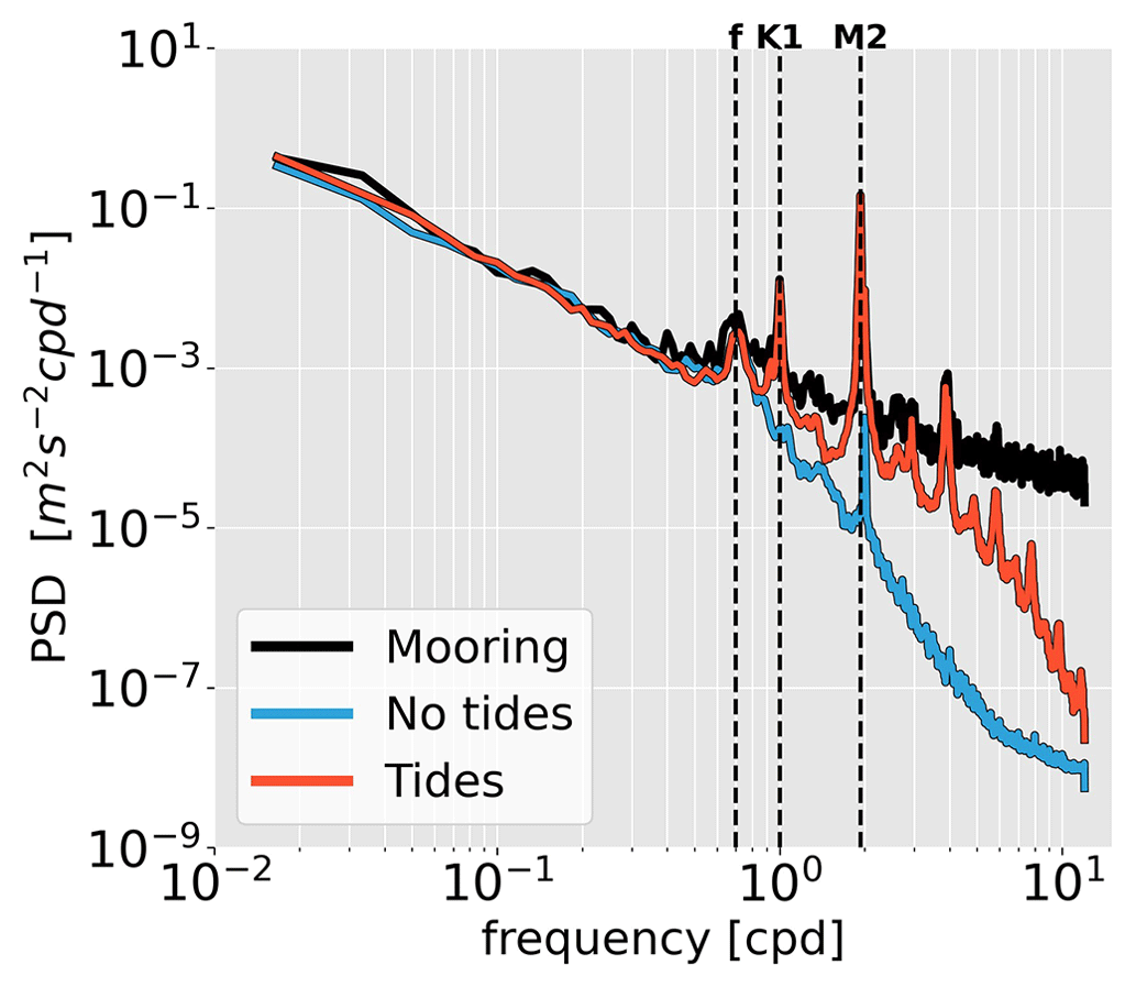
Figure 4 Power spectral density of near-surface (20–100 m) horizontal kinetic energy for CALEDO60 without (blue) and with (red) tidal forcing for the full-model time series near 167.25^∘ E, 20.43^∘ S in the New Caledonian eastern boundary current (see Fig. 3a). The energy spectra are compared to a mooring time series that was deployed between November 2010 and October 2011 (Durand et al., 2017). The vertical dashed black lines are representative of the inertial frequency f, the peak frequency of the K1 diurnal tide, and the peak frequency of the M2 semi-diurnal tide. Note that the signal at the semi-diurnal frequency (2 cpd) evident in the simulation with and without tides as well as in the mooring data is primarily linked to the atmospheric S2 tide, which is contained in the atmospheric forcing of ERA5 (not shown; Chapman and Lindzen, 1969; Balidakis et al., 2022).

3.3 Kinetic energy frequency spectra

In situ observations are also used to validate energy levels from seasonal down to tidal frequencies obtained from a full-year in situ current meter mooring (see Sect. 2.3.3, Fig. 4). Model energy levels are very close to observations from seasonal to inertial timescales (180 d to 36 h), i.e., for mesoscale and submesoscale processes. Inertial and tidal energy peaks are also in good agreement. For higher frequencies, the simulation with tidal forcing (red line) introduces a major improvement to the simulation without tidal forcing (blue line). This is especially true for the internal wave continuum raising the energy levels closer to the observations for frequencies >f. This validation, even if only performed at one location, gives us confidence in the ability of the numerical simulation to correctly represent the tides and their interaction with mesoscale processes.

3.4 Barotropic M2 tide validation

The barotropic tide in both the host grid (TROPICO12) and the nesting grid (CALEDO60) is compared with the empirical estimates from the barotropic tide model FES2014 (see Sect. 2.3.4) by applying a harmonic analysis to the full-model hourly SSH. Note that the daily output of the three-dimensional variables from TROPICO12 does not allow for a decomposition between the barotropic and baroclinic tide through the projection onto vertical modes. Therefore, we treat the full-model SSH as a proxy for the barotropic tide. For the sake of consistency, we treat CALEDO60 similarly. The M2 tides of TROPICO12 (Fig. 5a) and CALEDO60 (Fig. 5c) are in overall accordance with FES2014 (Fig. 5c and Fig. 5d, respectively). The amphidromic points are well located and amplitudes of SSH are of the same order of magnitude. Note that the modulations at shorter wavelengths in Fig. 5c and d are attributed to the baroclinic SSH signatures, which are presented at a later stage in Sect. 6.1.

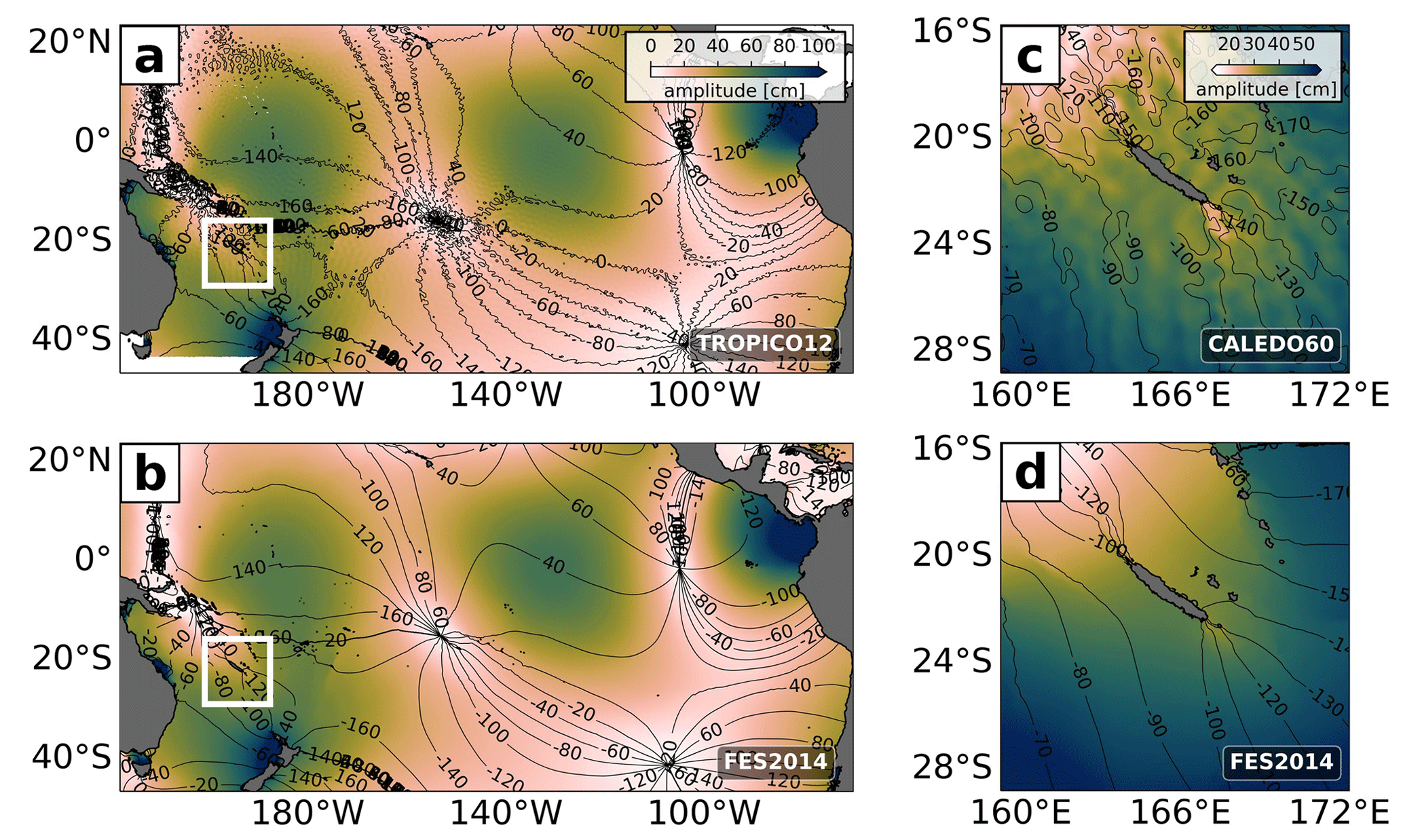
Figure 5 M2 SSH amplitude (shading) and phase (contour) for (a) TROPICO12 and (c) CALEDO60 based on a 1-year (2014) harmonic analysis (assuming that the model SSH is dominated by the barotropic tide) and in comparison to the global tide atlas FES2014 for (b) TROPICO12 and (d) CALEDO60. The boxes in (a) and (b) indicate the location of the CALEDO60 domain.

3.5 Stratification

Finally, in order to study internal-tide dynamics, a correct representation of the ocean's stratification is essential. Internal tides are expressed inter alia in the vertical displacement of isopycnal surfaces (Arbic et al., 2018), which can be decomposed by a sum of discrete baroclinic modes that only depend on buoyancy frequency and water depth (see Sect. 2.2.1). We compare the vertical hydrographic structure of CALEDO60 with a hydrographic climatology (CARS2009, see Sect. 2.3.1). The model mean density was horizontally binned to the climatological grid ($\mathrm{1}/{\mathrm{2}}^{\circ }$), whereas the climatological density was vertically interpolated onto the model grid. The water masses (not shown) and buoyancy frequency profiles correspond well to each other. An example of such a comparison is illustrated by looking at a stratification profile south of New Caledonia (166^∘ E, 26^∘ S, Fig. 6a). The maximum stratification around 100 m depth is slightly reduced in the model compared to climatology. This is attributed to a reduced salinity maximum in the thermocline in the model (not shown). The normalized modal structures for the four lowest modes and for both the displacement and vertical velocity (Fig. 6b) agree well with climatology. In particular, the depths of the zero crossings correspond well to each other.

Overall, we conclude that our model simulation is capable of realistically simulating both background ocean dynamics and internal tides. This encourages us to study the internal-tide field around New Caledonia in detail including its tidal energy budget, its vertical structure, and finally its SSH signature.

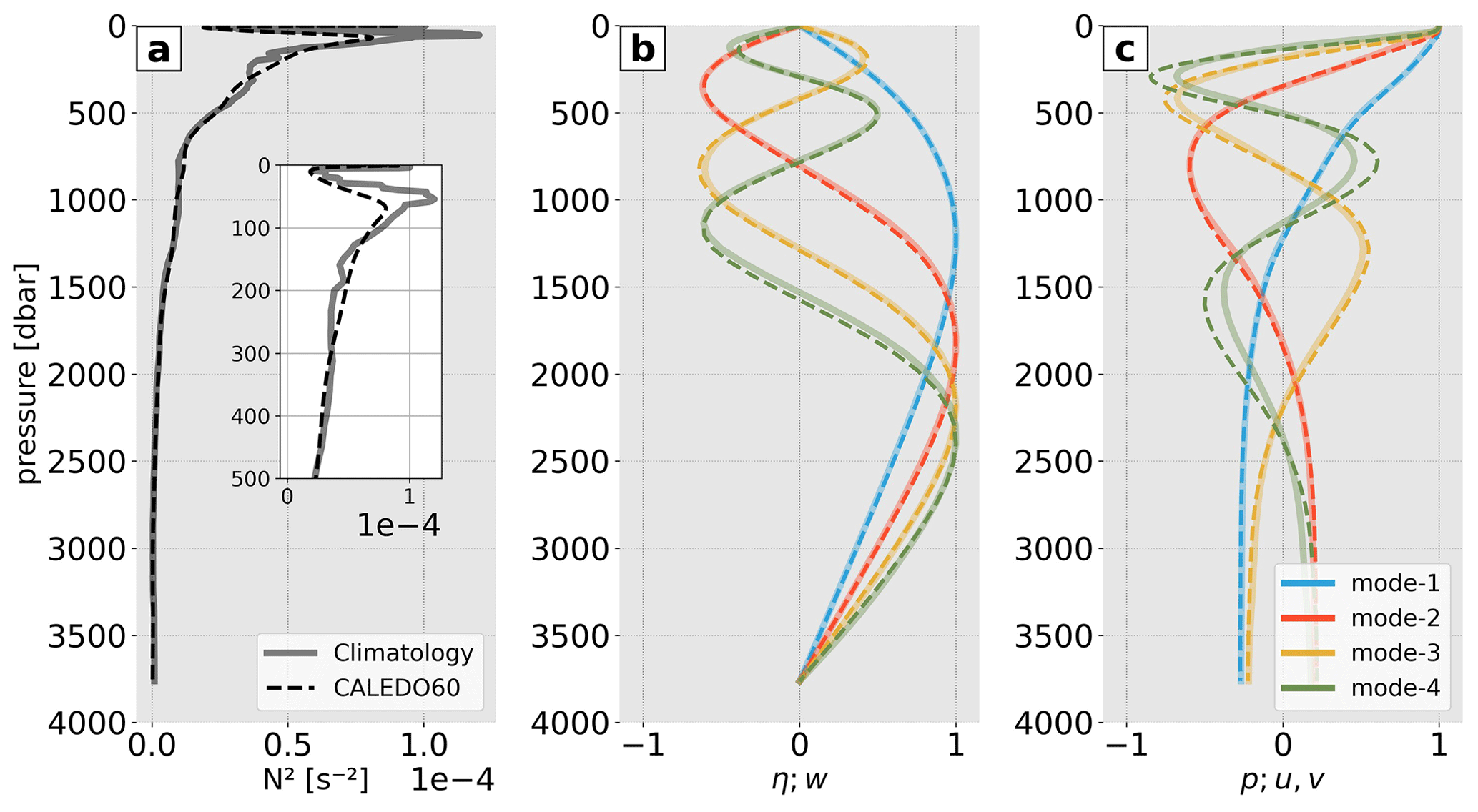
Figure 6 (a) Squared buoyancy frequency (N²) for a representative profile at 166^∘ E, 26^∘ S from the CARS2009 climatology (solid) and CALEDO60 (dashed). A zoom for the upper 500 m is given in the inset. Normalized baroclinic modal structures for (b) displacement η and vertical velocity w, as well as (c) pressure p and horizontal velocity u and v, for the four lowest modes are also shown.

4 Barotropic–baroclinic coherent M2 tide energy budget

In the following, we first analyze the M2 internal-tide field around New Caledonia by quantifying the energy conversion from the barotropic to the baroclinic tide while linking it to the local bathymetry. We also discuss the overall energy budget of the coherent M2 internal tide. We start with a regional overview before focusing on the regional hot spots of internal-tide generation.

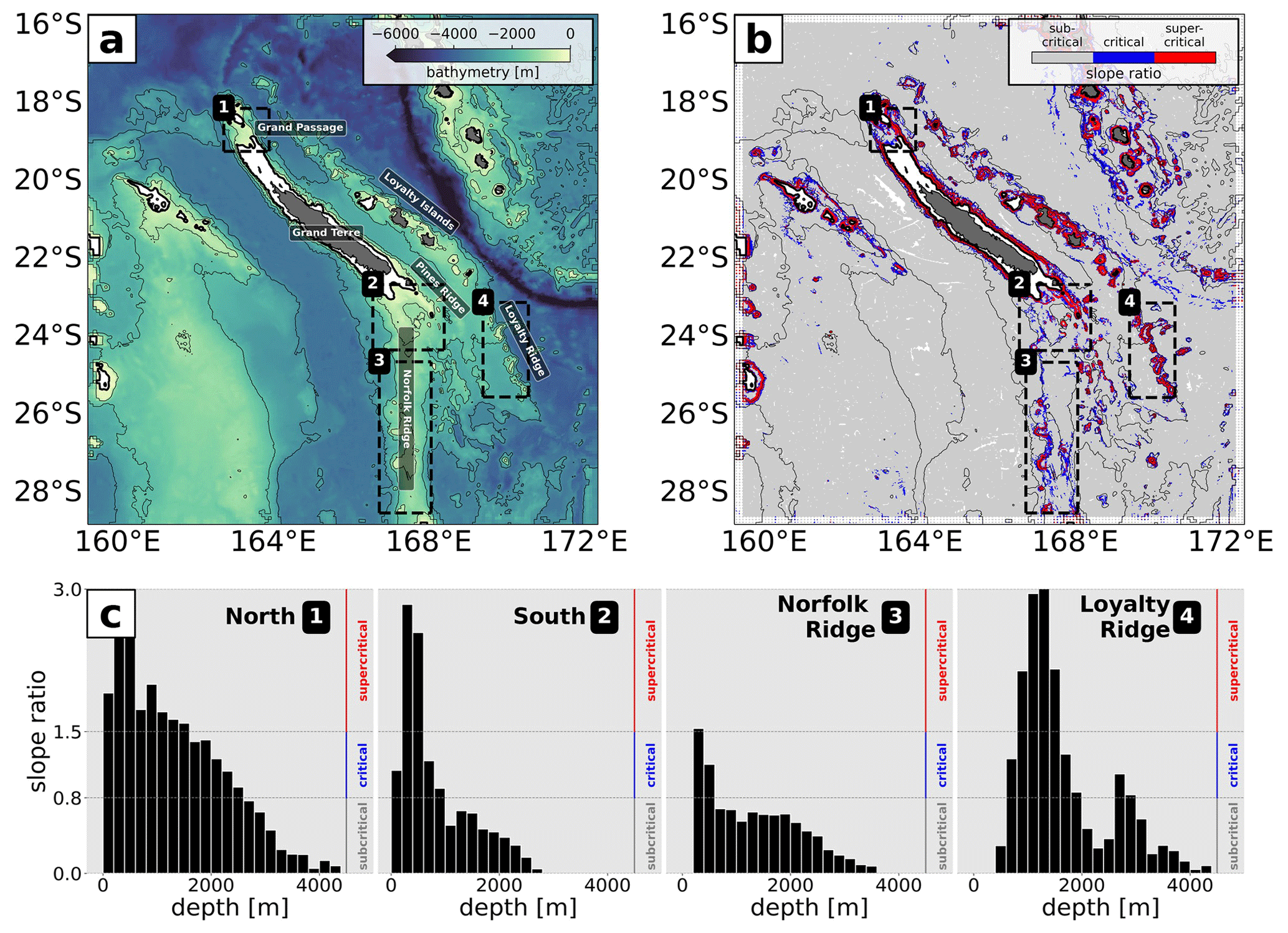
Figure 7 CALEDO60 (a) bathymetry and (b) M2 tide slope ratio α between topographic slope and wave slope s, divided into subcritical (gray, α<0.8 s), critical (blue, 0.8 s $<\mathit{\alpha }<\mathrm{1.5}$ s), and supercritical (red, α>1.5 s) slopes. Note that white shaded grid points are associated with a zero bathymetry gradient. The thin black lines represent the 1000, 2000, and 3000 m depth contours. The thick black line is the 100 m depth contour representative for the New Caledonian lagoon. The numbered black boxes represent the hot spots of internal-tide generation (1: North, 2: South, 3: Norfolk Ridge, 4: Loyalty Ridge) for which the distribution of the slope ratio as a function of depth (divided into 200 m depth bins) is given in (c).

4.1 Regional overview

Tidal energy conversion from the barotropic to baroclinic tide is closely linked to the bathymetry that is shortly presented in the following for the regional model domain (Fig. 7a). It is characterized by a complex northwest–southeast-extending ridge system, deep-reaching trenches, small-scale basins, seamounts, and shallow lagoons. The ridge system is composed of two major ridges, Norfolk Ridge and Loyalty Ridge. Norfolk Ridge extends from north of the Grand Passage all the way to the northern tip of New Zealand. The main New Caledonia island (Grande Terre) is located on the northern segment of Norfolk Ridge, also referred to as the New Caledonia Ridge. Loyalty Ridge stretches parallel to Norfolk Ridge, giving rise to the Loyalty Islands (Payri and de Forges, 2006). Seamounts are ubiquitous around New Caledonia and most prominent south of Grande Terre (Samadi et al., 2006).

As the M2 barotropic tidal energy flux curves southwestward around New Caledonia, the region is subject to barotropic-to-baroclinic energy conversion (Fig. 8a). Positive conversions represent energy transfer from the barotropic to the baroclinic tide; negative conversions are argued to be a measure of the energy transfer from the baroclinic tide to the barotropic tide due to pressure work (Zilberman et al., 2009). However, they may also reflect limitations in the baroclinic–barotropic decomposition (Lahaye et al., 2020). Thus, they remain difficult to explain physically and will not be further discussed here.

In the full-model domain, a total 21.16 GW of barotropic tidal energy is lost, 72 % (15.27 GW) of which is transferred to baroclinic tidal energy, whereas 28 % (5.89 GW) is dissipated due to bottom friction. This is a significant loss of barotropic tidal energy. For comparison, barotropic tidal energy loss has been estimated at 18.35 and 2.73 GW, 94 % and 84 % of which are converted to baroclinic tidal energy for the Luzon Strait (Kerry et al., 2013) and the Hawaiian Ridge (Carter et al., 2008), respectively.

In the whole domain (not shown), conversion is observed at all depths up to 4000 m and over a broad range of slopes. However, tidal conversion peaks in shallow waters with overall 25 % of the area-integrated energy that is associated with the upper 500 m. Moreover, two-thirds of the tidal conversion occurs on critical and supercritical slopes. Mode 1 clearly dominates, explaining almost 70 % of the total tidal energy conversion. Higher modes play only a minor role (15 % for mode 2 and 7 % for mode 3). For the whole domain, 93 % of this generated baroclinic energy is finally dissipated inside the domain, while little energy (1.06 GW) leaves the domain (Fig. 8a). Note that this quantity is representative of the net baroclinic flux of inward and outward energy propagation.

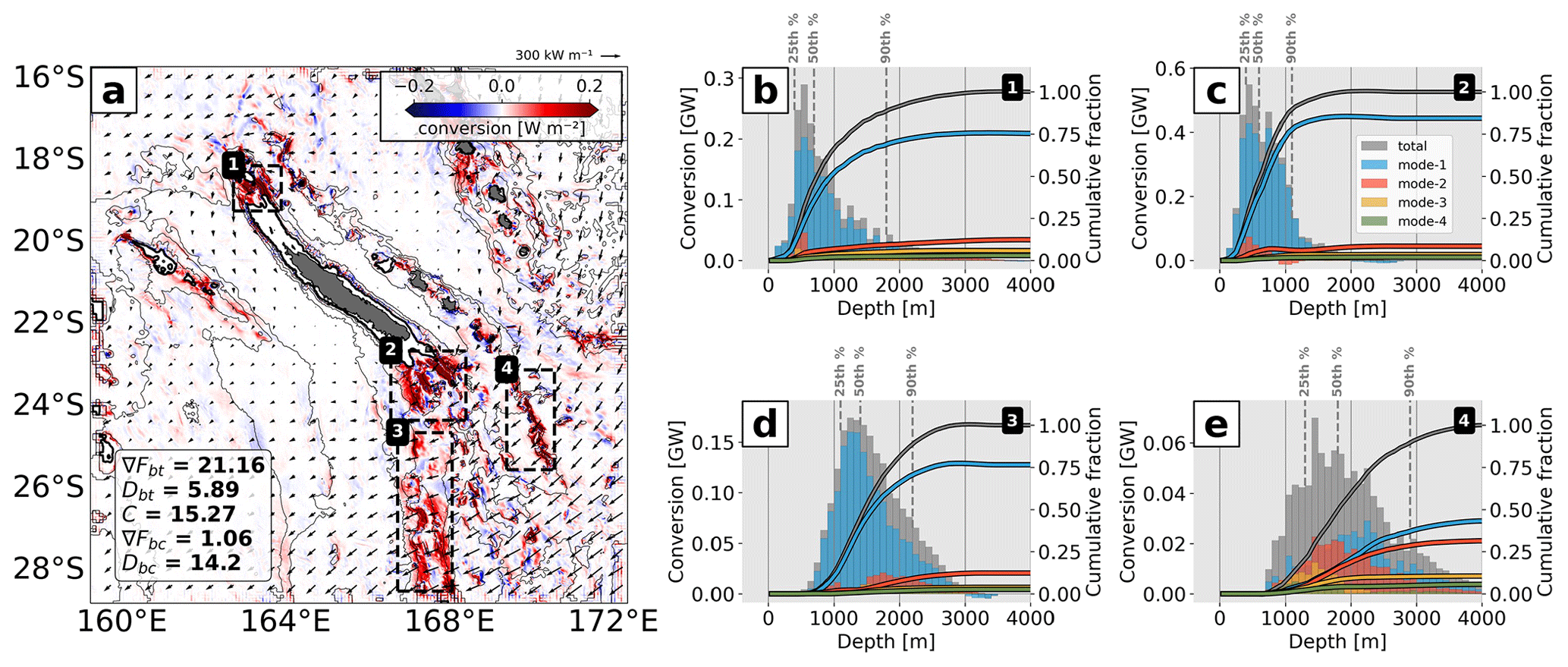
Figure 8 (a) M2 barotropic-to-baroclinic conversion including barotropic energy flux vectors and the full-domain area integral of the barotropic energy flux divergence (∇F_bt), barotropic energy dissipation (D_bt), barotropic-to-baroclinic conversion (C), baroclinic energy flux divergence (∇F_bc), and baroclinic energy dissipation (D_bc) in gigawatts (GW). Bathymetry contours and the black boxes are given as in Fig. 7. Histograms of the regional area-integrated conversion (total baroclinic and four lowest modes) as a function of generation depth divided into 100 m depth bins for (b) North (1), (c) South (2), (d) Norfolk Ridge (3), and (e) Loyalty Ridge (4). The 25th, 50th, and 90th percentiles as well as the normalized cumulative fraction are also shown.

4.2 Subregional analyses

Here, we identify four regions of internal-tide generation which together represent roughly 60 % of the full-domain area-integrated M2 barotropic-to-baroclinic conversion. These hot spots are illustrated by the black boxes in Fig. 7a–b and Fig. 8a and defined as North (1), South (2), Norfolk Ridge (3), and Loyalty Ridge (4). The conversion and energy budget are discussed for each area in light of its topographic characteristics (Fig. 7). The energy budget and the part dissipated locally are also provided for each subregion to better infer where the dissipation occurs and where tidal mixing is expected (Fig. 9, see also Table A1).

The North (1) domain is characterized by a very steep (with critical and supercritical slopes) shelf break at the eastern flank of the New Caledonia Ridge and a 500 m deep, 50 km wide passage (Grand Passage) that is located between the d'Entrecasteaux Reef and the main island reef (Fig. 7a–b). Two-thirds of the tidal energy conversion occurs at depths shallower than 500 m (Fig. 8b), predominantly on critical and supercritical slopes (Fig. 7b–c). The region features the highest dissipation rate of barotropic energy compared to the other three regions. Of the 3.83 GW that is lost by the barotropic tide, 1.66 GW (43 %) is directly lost through bottom friction (Fig. 9a). Of the 2.17 GW that is converted to baroclinic energy, 32 % (0.70 GW) dissipates locally, while the remaining 68 % (1.47 GW) radiates away.

The South (2) domain has similar bathymetric characteristics in terms of depth and slopes. It represents the southward extension of the New Caledonia Ridge, just south of the New Caledonian lagoon. The most prominent bathymetric feature is Pines Ridge: it is a very steep (critical and supercritical slopes) and narrow ridge (a few tens of kilometers wide) of 100 km length that may be as shallow as 500 m (Fig. 7a–b). This region will be analyzed in more detail in Sect. 4.5 since it is subject to the most intense energy conversion with a total of 3.92 GW (Fig. 9b), primarily in depths shallower than 500 m (Fig. 8c). Further, local dissipation is essentially higher than in the North (1) domain.

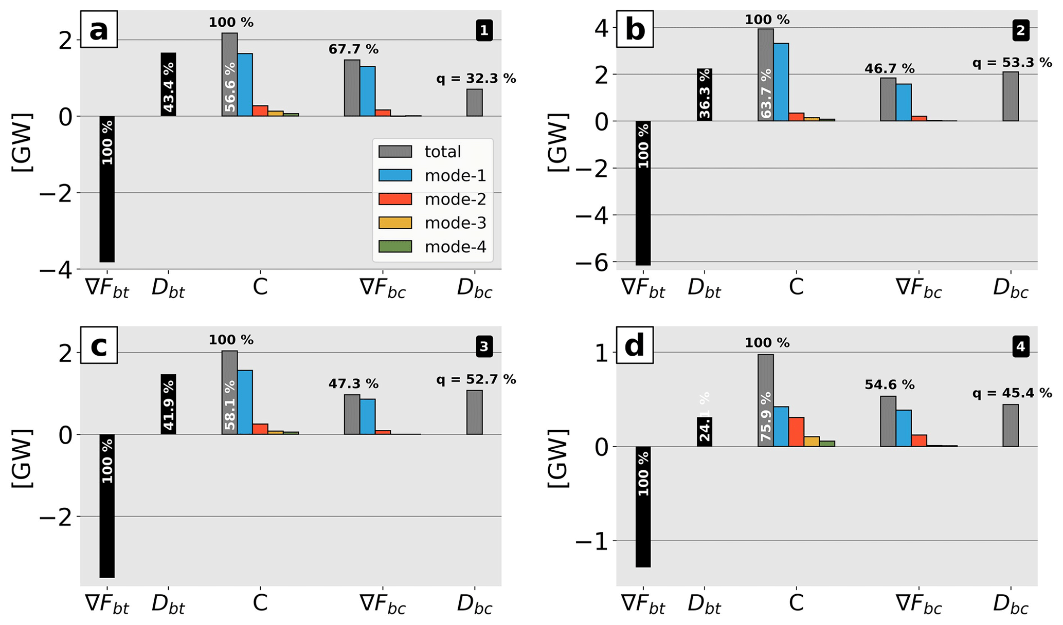
Figure 9 Bar plots of the regional barotropic–baroclinic M2 energy budgets for (a) North (1), (b) South (2), (c) Norfolk Ridge (3), and (d) Loyalty Ridge (4) including the barotropic energy flux divergence (∇F_bt) and barotropic energy dissipation (D_bt) as well as conversion (C) and baroclinic energy flux divergence (∇F_bc) for the total baroclinic and the four lowest modes. The baroclinic energy dissipation (D_bc) determined by the residual of ∇F_bc and C is also given. The percentage values (i) in white give the ratio of the barotropic energy flux divergence that is either dissipated through bottom friction or converted to baroclinic energy. The values (ii) in black give the ratio of the energy conversion term that is either radiated away or dissipated (q).

Norfolk Ridge (3) exhibits different bathymetric characteristics. It is defined as the >100 km wide north–south-stretching ridge between 24.5 and 28.5^∘ S. It is dominated by subcritical slopes at depths >1000 m (Fig. 7c) and also features steep (critical) slopes at mid-depths (400–700 m) which are mostly associated with seamounts. It is mainly characterized by energy conversion at subcritical slopes peaking at depths in the range 1000–2000 m with the 50th percentile at around 1500 m and the 90th percentile below 2000 m (Fig. 8d). Similarly to South (2), approximately half (53 %) of the converted baroclinic energy (2.04 GW) is dissipated locally (1.07 GW), while the other half (47 %) is radiated away (0.96 GW, Fig. 9c).

Loyalty Ridge (4) is a deep and narrow ridge composed of seamounts and guyots (Pelletier, 2007). These seamounts and guyots are located between 1000 and 2000 m depth, but deeper ones are also found between 2500 and 3000 m. They are characterized by supercritical and critical slopes, respectively (Fig. 7b–c). It features the most efficient energy conversion from the barotropic to baroclinic tide. Of the 1.28 GW that is lost by the barotropic tide, only 0.31 GW (24 %) is directly lost through bottom friction (Fig. 9d). The area-integrated baroclinic energy accounts for 0.97 GW, 45 % of which dissipates within the region (0.44 GW) and 55 % leaves the domain (0.53 GW).

Most of the tidal energy conversion discussed above is dominated by mode 1, explaining 75 %, 84 %, and 76 % for North (1), South (2), and Norfolk Ridge (3), respectively (Fig. 9a–c). In these, regions, mode 2 (7 %–12 %) and mode 3 (4 %–6 %) contribute little to the total baroclinic energy conversion. Loyalty Ridge (4) represents an exception with notable contributions of higher vertical modes: 43 %, 31 %, 11 %, and 6 % associated with mode 1 through mode 4, respectively (Fig. 9d).

These findings are partly consistent with the literature. In shallow depth ranges, the tidal energy conversion is expected to be largest for mode 1 (Falahat et al., 2014). Also, we expect mode 1 to be dominant for steep, tall, narrow structures such as in the North (1) and South (2) domains, similarly found for the Hawaiian Ridge (Laurent et al., 2003; Laurent and Nash, 2004). In the case of a deeper ocean bottom with small-scale bathymetric structures, such as Loyalty Ridge (4), higher modes are expected to become more important. The general presence of critical and subcritical slopes suggests a superposition of numerous vertical modes forming beams (Gerkema, 2001; Balmforth et al., 2002; Legg and Huijts, 2006). Nevertheless, we did not find any clear relationship between the bathymetric slope and excitement of vertical modes. The high dissipation rates in South (2) and Norfolk Ridge (3) could be explained by the successive bathymetric obstacles encountered by the internal-tide beams emanating from the generation spots with low modes scattered to higher modes before being dissipated locally (Lahaye et al., 2020). Surprisingly, the fraction of energy dissipation around Loyalty Ridge (4) is slightly reduced even though higher vertical modes are generated, which should imply more local dissipation.

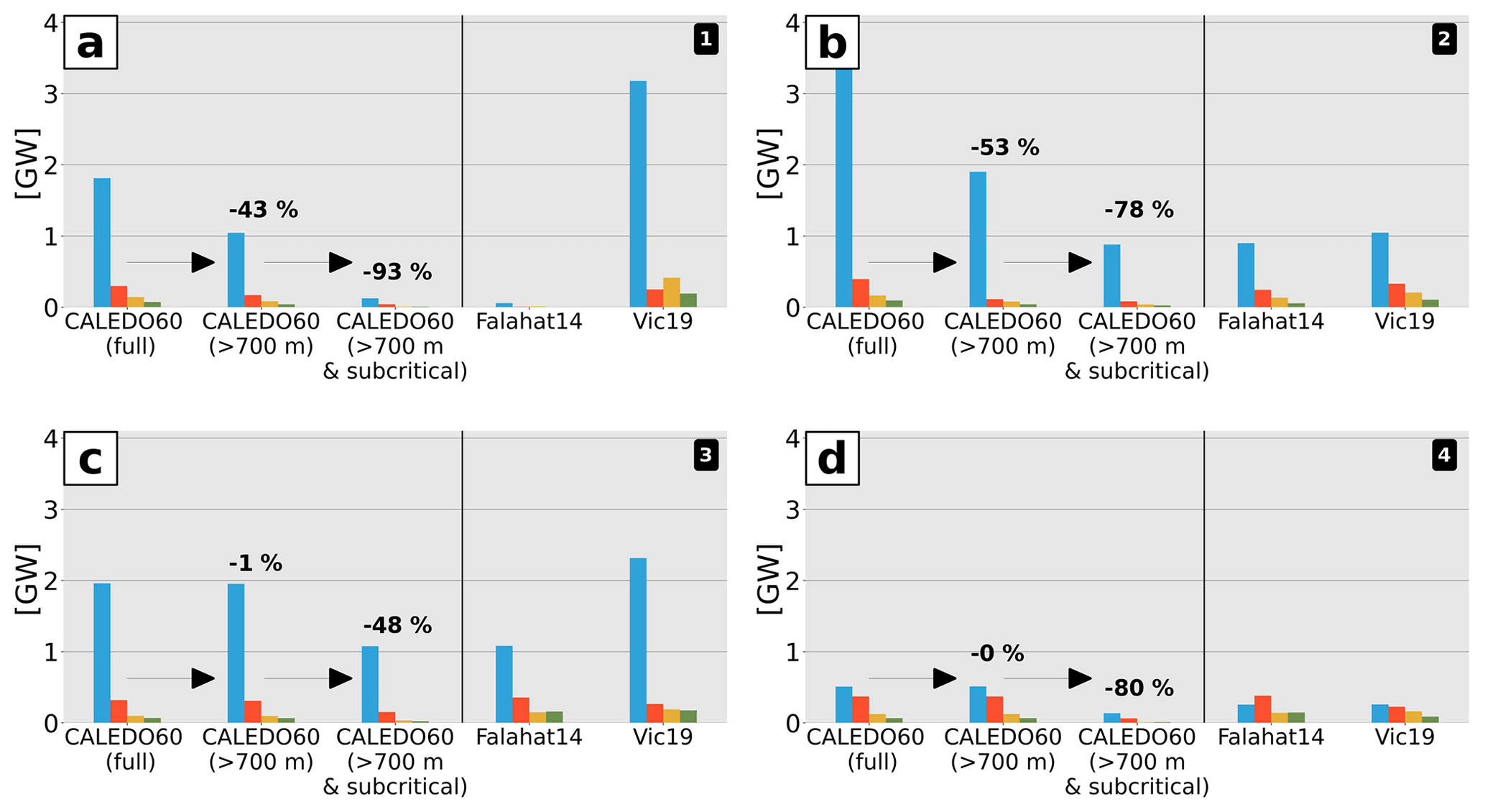
Figure 10 M2 barotropic-to-baroclinic energy conversion in gigawatts (GW) for the four lowest modes integrated over (a) North (1), (b) South (2), (c) Norfolk Ridge (3), and (d) Loyalty Ridge (4) for the full model, corrected for the upper 700 m, and corrected for both the upper 700 m and critical to supercritical slopes. The associated percentage decrease for the given correction is also shown. Energy conversion is compared to the semi-analytical estimates from Falahat et al. (2014) (Falahat14) and Vic et al. (2019) (Vic19) corrected for the upper 700 m. The color code is as in Fig. 9.

Briefly summarized, the bulk of energy conversion from the barotropic to the baroclinic tide is confined to four hot spot regions in shallow waters (500 m), closely linked to the complex bathymetry (i.e., shelf breaks, ridges, and seamounts), and dominated by mode 1. Approximately half of the locally generated energy dissipates in the near field, whereas the other half propagates outside the hot spot regions. This suggests a quick attenuation of baroclinic energy. Our model results show that the fraction of coherent internal tides that loses energy locally ($q=D_{\text{bc}}/C$) is elevated in our study region compared to 36 % and 20 % for the Luzon Strait (Kerry et al., 2013) and the Hawaiian Ridge (Carter et al., 2008), respectively. Potential factors that may contribute to this loss of energy will be discussed later in Sect. 6.2. Particularly, we will point out that the high dissipation rates observed in our analysis may not be solely associated with actual energy dissipation, but also with a loss of tidal coherence. This will be explored in more detail in Part 2 of this study.

4.3 Comparison with semi-analytical model estimates

In the following, we compare our M2 modal conversion for the four subregions with the semi-analytical model estimates from Falahat et al. (2014) (Falahat14) and Vic et al. (2019) (Vic19) in Fig. 10. Recall that both products represent the energy conversion in depths >700 m and on subcritical slopes only (see Sect. 2.3.6). The model conversion is given for the full model (considering the full water column and subcritical, critical, and supercritical slopes), the full model but only considering depths >700 m, and the full model but only considering both depths >700 m and subcritical slopes. The latter ensures the best comparison between the semi-analytical and numerical model estimates.

Overall, there is good agreement between our full-model estimates and those from semi-analytical theory concerning the conversion's modal content, with mode 1 being clearly dominant. Higher modes appear to only increase in relative importance for Loyalty Ridge (4) (Fig. 10d). The full-model energy conversion tends to be excessive in the South (2) domain (Fig. 10b). When correcting the full model for conversion in the upper 700 m in addition to conversion on critical and supercritical slopes, our model conversion compares better with the semi-analytical estimates. Even though corrected for the upper 700 m, there is no good comparison with Vic19 in the North (1) domain (Fig. 10a). This could be related to violation of linear theory that leads to unrealistic conversion rates larger than the energy lost by the barotropic tide. Remaining discrepancies among the products may be attributed to the associated bathymetry products that differ in both horizontal resolution and the correct representation of those bathymetric structures that are key for internal-tide generation.

While semi-analytical theory has proven very valuable in providing a first-order estimation of internal-tide generation on global scales, it reaches its limits in regions with shallow and complex bathymetry with critical to supercritical slopes. In fact, we find for the subregions around New Caledonia that roughly 50 %–90 % of the energy conversion may be missed locally when not allowing for conversion in the upper 700 m and on critical to supercritical slopes. This highlights the need for realistic, high-resolution numerical simulations to more faithfully represent the local internal-tide generation and dynamics.

4.4 Regional overview of tidal energy propagation and dissipation

The propagation of baroclinic tidal energy is expressed mainly by two predominant tidal beams that emerge from the North (1) and South (2) domains (Fig. 11a). They are 100–200 km in width and feature magnitudes well above 20 kW m⁻¹ (locally up to 30 kW m⁻¹) near the respective generation sites but propagate not more than 800 km toward the open ocean. In contrast to the southern tidal beam that propagates from its generation site at Pines Ridge southwestward and northeastward (though the northeastward beam is more limited), the northern tidal beam mainly propagates northeastward. This is attributed to the energy conversion that is confined to the shelf break east of the Grand Passage, whereas the Grand Passage itself is subject to only minor energy conversion (not shown). Tidal beams also emerge from Norfolk Ridge (3) and Loyalty Ridge (4). However, they are overall less pronounced and smaller in magnitude (5 kW m⁻¹).

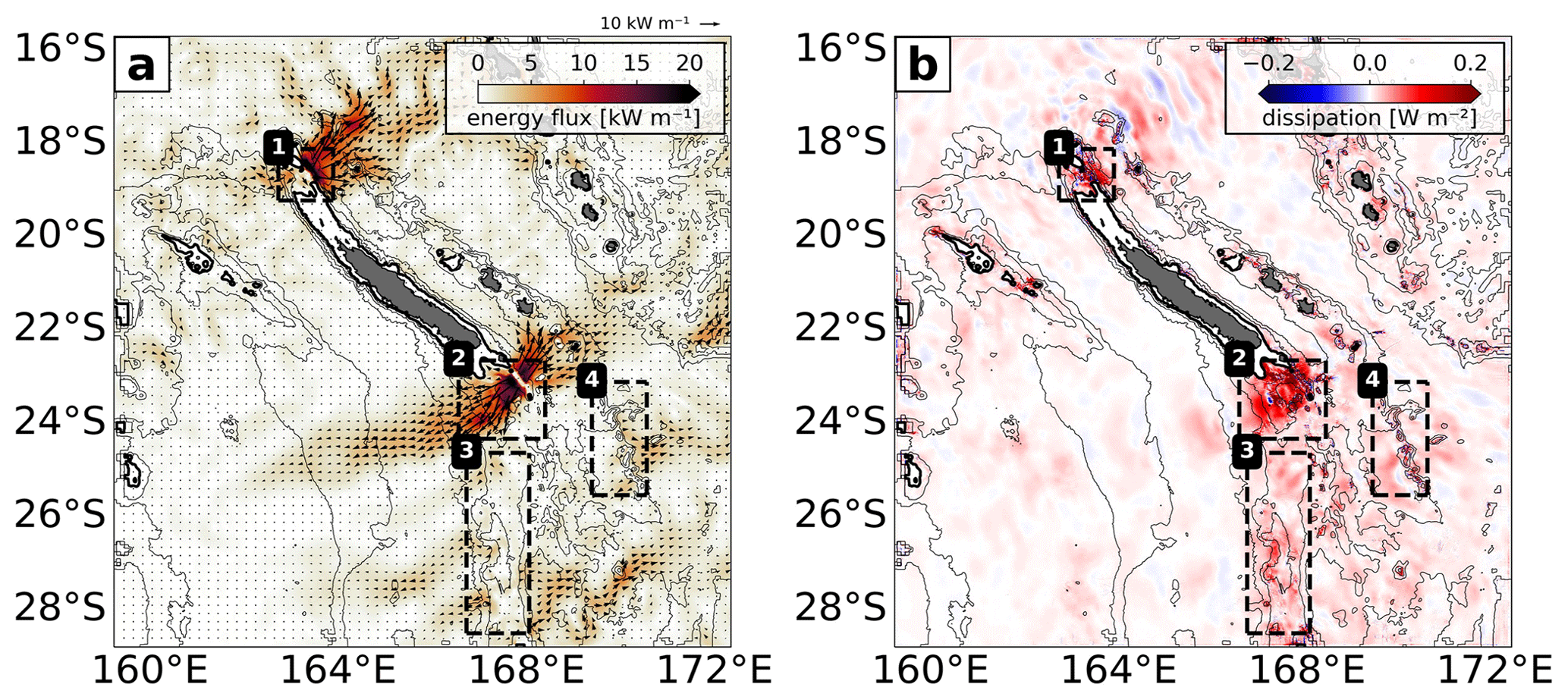
Figure 11 (a) M2 coherent energy flux (shading) including flux vectors. (b) M2 coherent energy dissipation (residual between the energy flux divergence and conversion). Bathymetry contours and the black boxes are given as in Fig. 7.

The rather quick attenuation of the tidal beams may be associated with the high dissipation rates, which are in large part constrained to the hot spot regions (Fig. 11b). This is reflected in the regional energy budgets and sheds light on the high fraction (∼50 %) between local energy dissipation and generation (see Sect. 4.2). Dissipation also occurs away from the hot spot regions, but to a lower degree.

4.5 Zoom-in of the South (2) domain

The South (2) domain deserves special attention for two reasons: first, it represents a study area of the SWOT–AdAC program accompanied by an extensive field campaign. This will be further addressed in Sect. 6.4. Second, it represents the predominant hot spot of internal-tide generation contributing more than 40 % and 25 % to the area-integrated barotropic-to-baroclinic energy conversion associated with the four subregions and full regional domain, respectively.

In total, 6.16 GW is lost by the barotropic tide, 64 % (3.92 GW) of which is converted to internal tides (Fig. 12a). The bulk of energy is generated when the incoming barotropic tidal flow encounters Pines Ridge, featuring conversion rates well above 1 W m⁻² on both its western and eastern flanks. Further internal-tide generation is localized downstream along a secondary ridge parallel to Pines Ridge and across the western shelf break. Locally, positive conversion is also evident around seamounts that are present in the area, namely, Munida, Antigonia, Jumeaux Est, and Stylaster.

In contrast to the conversion map which shows isolated spots, baroclinic energy dissipation is observed throughout the domain, accounting for a total of 2.09 GW (Fig. 12b). In other words, well above 50 % of the locally generated energy dissipates within the South (2) domain. Dissipation maxima are located near the generation sites such as Pines Ridge and around the seamounts with dissipation rates >0.5 W m⁻², i.e., around Munida, Brachiopode, Jumeaux Ouest, and Stylaster. Increased levels of dissipation are also found along the barrier reef that encloses the southern Caledonian lagoon. Further energy dissipation occurs uniformly westward and eastward of Pines Ridge across the shelf break with constant dissipation rates >0.1 W m⁻².

The non-dissipated energy propagates away from the main generation site within well-confined tidal beams in southwestern and northeastern directions characterized by energy fluxes >20 kW m⁻¹ which attenuate gradually to roughly 10 kW m⁻¹ within 100 km distance of the generation site in the annual mean. A net energy flux of 1.83 GW leaves the South (2) domain, accounting for 47 % of the locally generated baroclinic tidal energy.

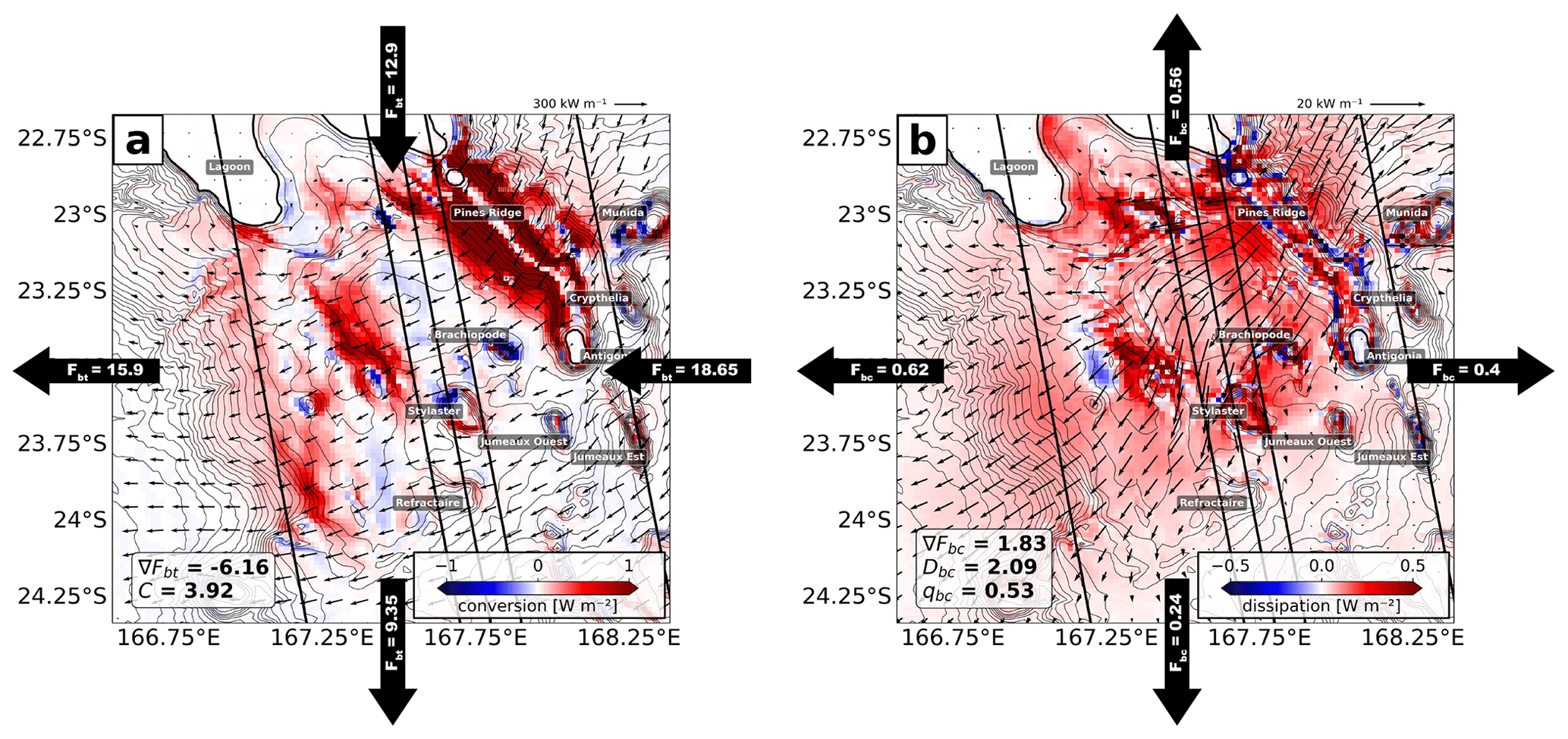
Figure 12 Regional M2 energy budget for the South (2) domain showing (a) the barotropic-to-baroclinic conversion (shading) overlaid by the barotropic energy flux (vectors) and (b) the depth-integrated baroclinic energy dissipation overlain by the depth-integrated baroclinic energy flux (vectors). The area-integrated values for the barotropic energy flux divergence (∇F_bt) and barotropic-to-baroclinic conversion C in (a) as well as the baroclinic energy flux divergence (∇F_bc), the baroclinic energy dissipation D_bc, and the ratio of locally dissipated baroclinic energy q_bc in (b) are also given. The incoming and outgoing (a) barotropic and (b) baroclinic energy fluxes with integrated values along the boundary are illustrated at the lateral boundaries of the domain, indicating the net direction of energy propagation. All integrated quantities are given in gigawatts (GW). Pines Ridge, the lagoon, and the most prominent seamounts are labeled. The depth contour interval is 100 m. The SWOT swaths and nadir track (solid black lines) during the fast sampling phase (1 d repeat orbit) are also shown.

5 Internal-tide SSH signature

The expression of internal tides in SSH is of major interest for SWOT observability of mesoscale to submesoscale dynamics. Here, we first investigate the M2 tide amplitude around New Caledonia before addressing the tidal signature in spectral space. The questions of interest are the following. (1) What are the processes in our study region that dominate the SSH signal in the mesoscale to submesoscale range? (2) What is the contribution of the coherent internal tide to these SSH signals? (3) To what extent are we able to increase observability of the mesoscale to submesoscale when correcting for the coherent internal tide?

5.1 SSH amplitude of the M2 internal tide around New Caledonia

We present the spatial maps of mode 1 and mode 2 of the M2 SSH amplitude in Fig. 13a and b in comparison with the satellite-altimetry-derived empirical estimates from the HRET model (see Sect. 2.3.5) in Fig. 13c and d for mode 1 and mode 2, respectively. Dominated by mode 1, the spatial distribution of SSH reveals multiple interference patterns with M2 tidal waves emanating from multiple generation sites and summing constructively and destructively as they propagate (Fig. 13a). Amplitudes may reach more than 6 cm in the internal-tide hot spot regions. Following a similar pattern but strongly reduced in amplitude, mode 2 features significant amplitudes of up to 2 cm at some locations. Overall, the M2 SSH signature resembles the energy flux in Fig. 11a with the predominant tidal beams to the north and south of New Caledonia. There is good agreement with the HRET model concerning the spatial representation of the M2 SSH for both mode 1 (Fig. 13c) and mode 2 (Fig. 13d). Overall, mode 1 seems to be enhanced in our model, whereas mode 2 is underestimated in some regions. Note that the given differences may be associated with the different time periods the datasets are referenced to as well as the length of the time series for the model (1 year) and altimetry (25 years).

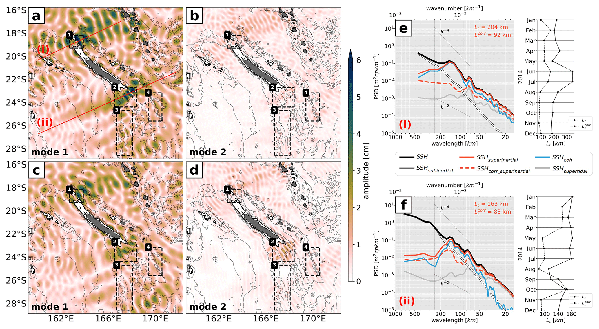
Figure 13 CALEDO60 M2 SSH amplitude for (a) mode 1 and (b) mode 2 in comparison with the empirical estimates of the High Resolution Empirical Tide (HRET) model for (c) mode 1 and (d) mode 2. Bathymetry contours and the black boxes are given as in Fig. 7. Annually averaged SSH wavenumber spectra for two transects (e) north and (f) south of New Caledonia, denoted (i) and (ii), respectively, in (a) (red lines). SSH spectra are presented for the altimetry-like SSH (corrected for the barotropic tide, SSH, black) with regard to the different dynamics that are separated in terms of frequency bands: subinertial (ω<f, SSH_subinertial, white) for mesoscale and submesoscale dynamics, as well as superinertial frequencies (ω>f, SSH_subinertial, solid red) for internal gravity waves decomposed into the coherent (SSH_coh, blue) internal-tide and supertidal frequencies ($\mathit{\omega }>\mathrm{1}/\mathrm{10}$ h, SSH_supertidal, gray). The altimetry-like SSH corrected for both the barotropic and baroclinic tide and filtered for motions at superinertial frequencies (SSH_{corr_superinertial}, dashed red) is also given. The characteristic wavenumber slopes k⁻² and k⁻⁴ are represented by the dotted black lines encompassing the mesoscale band (70–250 km, vertical dotted black lines). The transition scale L_t (i.e., where SSH_{superinertial} > SSH_subinertial) and the transition scale corrected for SSH_coh ($L_{\text{t}}^{\text{corr}}$, i.e., where SSH_{corr_superinertial} > SSH_subinertial) for the annually averaged SSH spectra are specified by the red numbers. The right sub-panels in (e) and (f) show the temporal evolution of L_t (solid) and $L_{\text{t}}^{\text{corr}}$ (dashed). These are computed similarly to the annually averaged SSH spectra above (i.e. SSH_{corr_superinertial} is still corrected for the annual coherent tide), but are determined by the monthly averaged spectra of SSH_{superinertial} $/$ SSH_{corr_superinertial} and SSH_subinertial.

5.2 SSH spectral signature

Wavenumber SSH spectra are commonly used to investigate dynamical regimes at work and to explore the relative importance of balanced and unbalanced motions which may feature similar wavelengths: the wavenumber slopes and relative levels of variance both provide information on these issues (e.g., Le Traon et al., 2008; Dufau et al., 2016; Savage et al., 2017; Tchilibou et al., 2020, 2022; Vergara et al., 2022, and many more).

Here the objective is to describe for two given transects in the tidal beam direction (red lines in Fig. 13a) the SSH signature with regard to the different dynamics that are separated in terms of frequency bands: subinertial frequencies (ω<f, SSH_subinertial) for mesoscale and submesoscale dynamics, as well as superinertial frequencies (ω>f, SSH_{superinertial}) for internal gravity waves while distinguishing between the coherent internal-tide (SSH_coh) and supertidal frequencies ($\mathit{\omega }>\mathrm{1}/\mathrm{10}$ h, SSH_supertidal).

Further, we will examine how SWOT observability may be limited in a region with strong internal tides. SWOT observability of mesoscale and submesoscale dynamics (balanced motion in this case) is ultimately governed by the transition scale L_t that separates balanced from unbalanced motion. The transition scale is a quantitative measure to estimate above which scales in spectral space the geostrophic balance is valid to derive balanced motion. Here, we define it as the intersection of subinertial and superinertial spectra. In other words, the transition scale is set to wavelengths where subinertial variance equals superinertial variance.

For both regions, subinertial processes explain almost all of the SSH variance for scales larger than 200 km (Fig. 13e, f). For scales smaller than 200 km, SSH variance is governed by superinertial processes, which are largely dominated by the coherent internal tide clearly expressed in spectral space with mode 1 and mode 2 around 160 and 80 km wavelength. In the annual mean, L_t is set to (i) 204 km and (ii) 163 km, meaning that the observability of balanced motion is largely limited below these scales as unbalanced motion dominates the SSH variance.

The correction of the total SSH for the coherent internal tide may be a promising attempt to assess balanced SSH dynamics. Doing so, L_t is reduced (i) from 204 km to 92 km and (ii) from 163 to 83 km. The right sub-panels of Fig. 13e and Fig. 13f show the monthly evolution of L_t and the corrected transition scale $L_{\text{t}}^{\text{corr}}$ over 1 model year. Temporal variations of the transition scale may be the result of the relative importance of subinertial motion, which undergoes seasonal variability (Callies et al., 2015; Rocha et al., 2016). This was explicitly shown for New Caledonia by Sérazin et al. (2020), who attributed the increasing importance of mixed layer instabilities and frontogenesis to more available potential energy in the Southern Hemisphere winter months.

Other temporal variations of the transition scale may be related to temporal variability of the internal tide. The coherent internal tide is by definition constant, but the incoherent internal tide (not shown here) depends on the seasonally varying stratification (Lahaye et al., 2019) and/or the interaction with the background currents (see Sect. 1 for references). Moreover, the incoherent signal remains in the corrected SSH signal. Therefore, the extent to which we can increase observability of mesoscale and submesoscale dynamics in areas with internal-tide activity depends on the amplitude of the incoherent internal tide. Understanding the temporal variations of the transition scale, its link to the incoherent internal tide, and its implication for SWOT SSH measurements is beyond this scope of this paper's objective, but it will be specifically addressed in Part 2.

Briefly, the dominance of unbalanced motion in the mesoscale to submesoscale band strongly restricts SSH observability of geostrophic dynamics to large eddy scales in our study regions. However, a correction for the coherent internal tide may improve the observability to well below 100 km.

6 Summary and discussion

Prominent topographic structures such as oceanic ridges, continental shelf breaks, seamounts, and island chains give rise to major internal-tide formation in large parts of the Pacific Ocean (Niwa and Hibiya, 2001). The majority of recent studies on internal tides focused mainly on two regions: the Luzon Strait (e.g., Niwa and Hibiya, 2004; Alford et al., 2011; Kerry et al., 2013) and the Hawaiian Ridge (e.g., Merrifield and Holloway, 2002; Zaron and Egbert, 2006; Carter et al., 2008). Here, we present for the first time the internal-tide dynamics around New Caledonia in the southwestern tropical Pacific Ocean using the output of a tailored high-resolution regional numerical model. Being subject to strong internal tides and elevated mesoscale eddy activity, New Caledonia represents an area of high interest for the upcoming SWOT altimeter mission to evaluate observability of mesoscale and submesoscale dynamics in the presence of unbalanced motion at wavelengths of similar scale. This is primarily true for the SWOT fast sampling phase, when the satellite sampled this region of interest every day. In this context, a dedicated field campaign (SWOTALIS, March–April 2023) was carried out in the framework of the SWOT–AdAC program (Morrow et al., 2019; d’Ovidio et al., 2019). The model results we obtained provide new and key information for the New Caledonia study region, but also more globally for the understanding of the generation and life cycle of internal tides. We were also able to gain insights into SWOT observability in a challenging region with strong internal tidal waves. These findings are summarized and discussed below.

6.1 New Caledonia: a hot spot of mode-1 internal-tide generation in the Pacific

The barotropic and baroclinic energy budget of the dominant M2 tide shows that in the regional model domain surrounding New Caledonia, 21.16 GW of the barotropic tidal energy is lost, 72 % (15.27 GW) of which is converted into baroclinic tidal energy. The main conversion zones are associated with the most prominent bathymetric structures such as the Grand Passage (2.17 GW) and Pines Ridge (3.92 GW) north and south of New Caledonia, respectively. This confirms that New Caledonia is a hot spot of internal-tide generation. The amount of energy converted is comparable to what has been estimated in the Luzon Strait (Kerry et al., 2013) and the Hawaiian Ridge (Carter et al., 2008), taking into account that the exact numbers depend on the size of the domain. The area-integrated M2 conversion is estimated as 15.27 GW around New Caledonia, 16.97 GW in the Luzon Strait, and 2.34 GW along the Hawaiian Ridge. Conversion integrated in the smaller subregions North (1) and South (2) are similar to the Hawaiian Ridge (2.17 and 3.92 GW, respectively). Local conversion rates are of the same order of magnitude (well above 1 W m⁻²) among all regions. Further, all regions feature similar energy propagating away from the formation site within well-defined tidal beams. Maximum M2 baroclinic energy fluxes vary from 10 kW m⁻¹ at the Hawaiian Ridge up to 30 kW m⁻¹ around New Caledonia and 40 kW m⁻¹ at the Luzon Strait.

Interestingly, the New Caledonia region stands out compared to other previously studied regions in terms of modal content. Our modeling results suggest that barotropic tidal energy is converted, overwhelmingly, into baroclinic mode 1 (75 % of the full-domain energy conversion and up 85 % in the South (2) domain). Modes 2–4 represent a comparable amount of energy only at Loyalty Ridge (4) characterized by deep topography. For comparison, this mode-1 conversion percentage was estimated to be around 30 % at global scale, 35 % for the Pacific basin (Falahat et al., 2014; Vic et al., 2019), 30 %–60 % around Hawaii (Merrifield and Holloway, 2002; Zilberman et al., 2011), and about 9 % over the northern Atlantic Ridge (Vic et al., 2018). The reasons behind this strongly dominant mode 1 are not completely understood. A dominance of mode 1 in the western Pacific has been previously suggested with semi-analytical models (Falahat et al., 2014; Vic et al., 2019), but not to that extent. Mode 1 has been suggested to be dominantly generated in shallow depths (Falahat et al., 2014). Apart from topographic characteristics such as height, width, and depth (Legg and Huijts, 2006; Falahat et al., 2014), the modal content is argued to be primarily governed by roughness and, thus, by the topography's spectral shape (Laurent and Nash, 2004). On the other hand, it has been observed and argued by many that critical and supercritical slopes are conducive to beam-like patterns, requiring the presence of higher vertical modes (Gerkema, 2001; Balmforth et al., 2002; Legg and Huijts, 2006). Fully understanding the strong dominance of mode 1 in our region characterized by the presence of steep, tall, and shallow ridges with critical and supercritical slopes, as well as 25 % of the conversion taking place above 500 m, would require further analyses.

An important lesson learned is that New Caledonia represents a complex area for linear semi-analytical models that break down for critical and supercritical slopes and shallow bathymetry, which in turn are key for internal-tide generation at our study site. Such semi-analytical models, although very useful and widely used to estimate tidal energy conversion, its modal distribution, and tidal mixing (e.g., Falahat et al., 2014; Vic et al., 2019; de Lavergne et al., 2019, 2020), miss a significant part of the conversion (50 %–90 %) in our area, pointing out the limitation of these approaches in such complex areas. This issue was also presented in Buijsman et al. (2020). However, it was only addressed on global scales, highlighting the relevance of realistic numerical simulations on regional scales.

6.2 A hot spot of internal-tide dissipation

Our model results suggest elevated ratios (q) between local tidal energy dissipation and generation of ∼50 % compared to other internal-tide generation hot spots in the Luzon Strait (36 %, Kerry et al., 2013) and the Hawaiian Ridge (20 %, Carter et al., 2008). This is surprising considering the clear dominance of mode 1 in most parts of our nesting model domain where mode 1 dominates the baroclinic tidal energy propagation. Nonetheless, the elevated levels of local energy dissipation provide an explanation for the relatively small propagation distance of the tidal beams (e.g., around 800 km for the tidal beam emanating from South (2)), essentially smaller compared to the tidal beams emanating from the Luzon Strait and the Hawaiian Ridge that may propagate several thousand kilometers toward the open ocean. Several processes of tidal energy dissipation have been discussed in the literature that are well summarized in de Lavergne et al. (2019, 2020): nonlinear wave–wave interactions, wave breaking through shoaling, dissipation on critical slopes, and scattering by abyssal hills. The interaction with the topography may explain the largest fraction of energy dissipation (Kelly et al., 2013). This especially concerns the scattering and energy transfer of the low-mode internal tide to higher modes leading to increasing dissipation. Nonlinear wave–wave interactions were shown to facilitate the energy transfer of low-mode internal tides to both superharmonic (Baker and Sutherland, 2020; Sutherland and Dhaliwal, 2022) and subharmonic frequencies (Ansong et al., 2018; Olbers et al., 2020). Particularly the latter, which is associated with parametric subharmonic instability, can be an important energy sink for low-mode internal tides near the critical latitude band (around 29^∘ N/S for the semi-diurnal tide) south of New Caledonia. The mechanisms of tidal energy dissipation and their relative contributions in our study area remain an open question. This is beyond the scope of this study and requires further investigation.

Recall that here the tidal energy dissipation (residual between energy flux divergence and conversion) corresponds to a coherent tidal analysis. Due to the length of the harmonically analyzed time series (full-model calendar year), it must be assumed that a non-negligible fraction of the coherent dissipation is not associated with true dissipation but with a loss of coherence or scattering of energy to the incoherent tide, i.e., with increasing distance from the internal-tide generation site (Rainville and Pinkel, 2006; Alford et al., 2019). The actual fraction of true energy dissipation will be addressed in more detail in Part 2 of this study involving the full semi-diurnal signal and tidal incoherence. A potentially important contribution to elevated dissipation rates could also be linked to the chosen bottom friction and drag parameterization (see Sect. 2.1). The tidal dissipation’s sensitivity to the given parameterization, however, was not addressed and would require a dedicated analysis.

6.3 A challenging spot for SWOT observability

The SWOT mission is dedicated to documenting two-dimensional fine-scale features down to 15 km wavelength that include both subinertial (mesoscale to submesoscale dynamics) and superinertial (such as internal tides) frequencies. Disentangling these different dynamics in terms of SSH is of interest for SWOT observability. Here, we have investigated the transition scale that separates the larger scale dominated by balanced geostrophic motion from the smaller scale dominated by unbalanced wave motions in the two main pathways of the internal-tide energy flux. Further, we analyzed what impact the correction for the coherent tide in the SSH signal has on the transition scale.

Wavenumber spectra of SSH reveal the dominance of unbalanced, rapidly changing motion, largely governed by the internal tide, in the mesoscale band at spectral wavelengths below 200 km. The separation length scale between balanced and unbalanced motion is in good agreement with estimates deduced from along-track satellite altimetry in Vergara et al. (2022, see their Fig. 6). Our findings also align with the global model analysis from Qiu et al. (2018), where the SSH-derived transition scale is estimated to be slightly below 200 and 160 km north and south of New Caledonia, respectively.

Correcting our model for the coherent internal tide, we are able to improve the observability of mesoscale and submesoscale SSH around New Caledonia to well below 100 km in the annual mean. The limited observability even after the correction of the coherent internal tide is potentially linked to the temporally varying tide. The study region may be subject to strong interactions between internal tides and mesoscale eddies, giving rise to tidal incoherence. This is especially true south of the New Caledonia that is characterized by elevated levels of EKE (see Fig. 3).

6.4 Perspectives of this work

This work is the first modeling approach to characterize the internal-tide dynamics around New Caledonia. Part 1 focuses on the coherent part of the main M2 component. Giving first insight into internal-tide generation, propagation, and dissipation as well as SSH observability, this study is meant to serve as a basis for future studies such as eddy–internal-tide interactions and their expression in SSH. Internal tides may be strongly sensitive to the background currents both at the generation sites and along propagation, with implications for tidal energy conversion from the barotropic to baroclinic tide and tidal energy dissipation. This will be the subject of Part 2 of this study. Further, a twin simulation experiment, with the same forcing and parameterizations but without tidal forcing, has been performed. Comparing the two simulations will help us understand how tides impact the mesoscale and submesoscale fields, as well as the forward and inverse energy cascades among spatial scales (work in progress).

The results obtained will play an important role when confronted with in situ observations. The dedicated SWOTALIS in situ experiment was carried out in March–May 2023 during the SWOT fast sampling phase (related to SWOT–AdAC) beneath the SWOT swaths and nadir track. Observational platforms such as moorings, repeated hydrographic sections, and long fixed stations spanning several semi-diurnal tidal cycles with microstructure measurements in the hot spots of internal-tide generation and dissipation as well as in the propagation direction will provide further insight into the internal-tide life cycle south of New Caledonia, in combination with the SWOT data. Our simulations will help link the full water column dynamics and the SSH measurements.

Finally, this study provided first hints on internal-tide dissipation spatial variability. Yet, the impact of tidally driven mixing on temperature, other tracer fields, and biological variables in this area of high biodiversity remains to be quantified. It is expected that strong vertical velocities along bathymetric slopes, reefs, and seamounts may influence nutrient inputs into the euphotic layer and primary production, potentially up to high trophic levels and marine fauna (Derville et al., 2020). Such effort has been recently initialized in the framework of the ScInObs (Science, Innovation and Observatories of seamounts) project led by the French Research Institute for Exploitation of the Sea (IFREMER) and in collaboration with the Japan Agency for Marine–Earth Science and Technology (JAMSTEC) south of New Caledonia at the Stylaster seamount (Fig. 12). Overall, observing and understanding the local impact of internal tides on the ecosystem are of large socioeconomic interest for the island's conservation management. We hope that our results will pave the way to a better understanding of the processes and ultimately help marine conservation.

Appendix A

Table A1 Regional M2 barotropic energy flux divergence ∇F_bt, barotropic energy dissipation D_bt, barotropic-to-baroclinic conversion C, baroclinic energy flux divergence ∇F_bc, and baroclinic dissipation D_bc integrated over the North (1), South (2), Norfolk Ridge (3), and Loyalty Ridge (4) domains. The vertical structures for modes 1–4 are given for C and ∇F_bc.

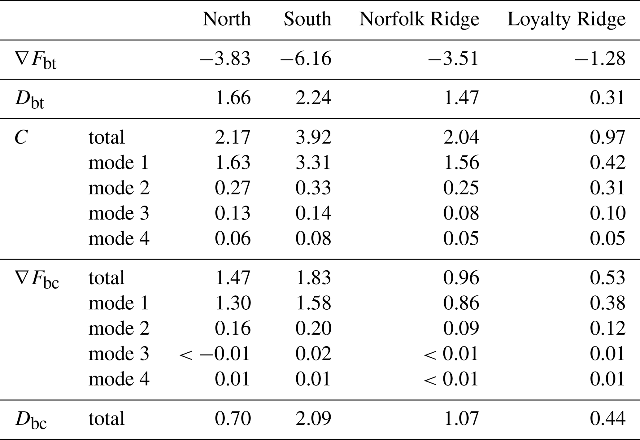
All units are given in gigawatts (GW).