Revisited heat budget and probability distributions of turbulent heat fluxes in the Mediterranean Sea

Understanding the surface heat budget of the Mediterranean Sea is essential for assessing its role in regional climate and ocean circulation. Under the steady-state heat budget closure hypothesis, the Mediterranean should exhibit a net surface heat loss to balance the heat gained through the inflow of warm Atlantic water at the Gibraltar Strait. However, literature estimates of the net heat flux vary widely, raising questions about the accuracy of existing reanalysis products. In this study, we compute the net surface heat flux over the Mediterranean using two atmospheric datasets: high-resolution (0.125°) ECMWF analysis and lower-resolution (0.25°) ERA5 reanalysis. By applying the same sea surface temperature fields and bulk formulas in both cases, we isolate the impact of atmospheric resolution and data quality. We find that the ECMWF analysis yields a basin-averaged net heat flux of $-\mathrm{3.6}\pm \mathrm{1.3}$ W m⁻², consistent with the closure hypothesis, while ERA5 gives a spurious positive flux of $+\mathrm{5}\pm \mathrm{1.2}$ W m⁻². Furthermore, beyond simply assessing the net heat budget, this study delves into the probability distributions of air–sea heat fluxes, aiming to gain a deeper understanding of associated uncertainties and extreme values in turbulent heat fluxes. The probability distributions for turbulent heat flux components exhibit characteristics such as skewness and kurtosis, respectively, varying across the basin. To assess the influence of extremes, we apply the Interquartile Range (IQR) method within statistical models that account for the skewed nature of turbulent heat flux distributions, enabling a consistent treatment of outliers. Our results reveal that extreme negative heat flux events play a critical role in determining the net heat flux direction; excluding these extremes leads to a spurious positive heat budget. Only ECMWF fields are consistent with the heat budget closure hypothesis. Furthermore, we demonstrate that the Mediterranean heat budget closure hypothesis is connected to extreme heat loss events occurring in key regions of the basin, such as the Gulf of Lion, the Adriatic Sea, the Aegean Sea, and the southern Turkish coasts.

1 Introduction

The exchange of momentum, water, and heat between the atmosphere and ocean plays a pivotal role in connecting their dynamics (Kara et al., 2000). These fluxes, influenced by atmospheric surface variables and Sea Surface Temperature (SST), drive ocean circulation (Large and Yeager, 2009; Small et al., 2019).

Our study focuses on the Mediterranean Sea, a unique semi-enclosed anti-estuarine basin where heat, water, and momentum fluxes intertwine to fuel a robust vertical circulation (Pinardi et al., 2019). The Mediterranean heat budget comprises of two main terms- the basin averaged surface and lateral boundary heat fluxes. Large uncertainties are associated with surface heat fluxes at different temporal scales (Jordá et al., 2017). We aim to reassess the long term mean net heat flux of the basin since this flux is a source of energy for the basin wide circulation (Cessi et al., 2014).

Understanding the heat budget in the Mediterranean Sea has long been a formidable task (Bignami et al., 1995; Castellari et al., 1998; Matsoukas et al., 2005; Pettenuzzo et al., 2010; Sanchez-Gomez et al., 2011; Criado-Aldeanueva et al., 2012; Jordá et al., 2017), whether through numerical models or observational data analysis. The fundamental challenge of in-situ observations is their limited spatial and temporal coverage, while numerical modelling is constrained by the semi-empirical nature of air–sea bulk formulas. Numerous endeavours have been undertaken (Large and Yeager, 2009) to calculate air–sea heat fluxes using atmospheric state variables obtained from in-situ observations, remote sensing data, or numerical model outputs. In this study, we utilize atmospheric analysis and reanalysis data, which provide an optimal reconstruction of past atmospheric surface state variables using models and observations. Furthermore, the estimate of the Mediterranean Sea heat budget from ECMWF meteorological analysis data sets has not been done before.

Numerous past studies have employed well-established bulk transfer formulas to estimate air–sea fluxes (e.g., Fairall et al., 2003; Pettenuzzo et al., 2010; Cronin et al., 2019). The turbulent heat flux components (latent and sensible heat flux) are commonly derived from surface wind speed, sea surface temperature, near-surface air temperature, and humidity (Large and Yeager, 2009). Gulev and Belyaev (2012) noted that global heat flux products often vary significantly, mainly due to differences in the bulk formulations and input variables adopted across studies.

At the Gibraltar Strait, the Mediterranean Sea exchanges water with the Atlantic through a characteristic two-layer flow: warm, relatively fresh Atlantic water enters at the surface, while colder, saltier Mediterranean water exits at depth leading to a net heat gain for the Mediterranean basin. To maintain a steady state balance in the basin averaged heat balance, this lateral heat gain must be compensated by a net loss of heat at the sea surface. In other words, the basin-average surface heat flux should be negative – a constraint known as the heat budget closure hypothesis. Accurately estimating this surface heat flux remains a challenge due to limited data and uncertainties in flux parameterizations. A benchmark estimates of the net heat budget, −7 W m⁻², was proposed by Béthoux et al. (1998), though it is based on data from the 1970s and 1980s and may not reflect present-day conditions under a changing climate (Criado-Aldeanueva et al., 2012; Marullo et al., 2021). We realise that assuming perfect balance between lateral and vertical heat fluxes, even in the Mediterranean Sea, is an approximation. Being heat clearly entering the Mediterranean Sea through Gibraltar, we search for a negative net heat flux, which we call the closure hypothesis. How negative such net heat flux is, we do not know but searching for a negative value is a conservative assumption aligned with current scientific understanding.

Recent studies highlight significant uncertainty in the estimated long-term net heat budget of the Mediterranean Sea, with some even reporting positive values. Song and Yu (2017), presented an ensemble climatology of surface heat fluxes, reporting a net heat budget of 2±12 W m⁻² and noting a warm bias in this ensemble estimate. Utilizing an ensemble of high-resolution regional climate models (RCMs), Sanchez-Gomez et al. (2011) found that individual RCMs did not achieve a heat budget closure, but the ensemble mean heat flux was $-\mathrm{7}\pm \mathrm{21}$ W m⁻². Using downscaled NCEP/NCAR global reanalysis of $\mathrm{1}/\mathrm{2}\mathit{°}\times \mathrm{1}/\mathrm{2}\mathit{°}$ resolution, Ruiz et al. (2008) computed a net heat budget of −1 W m⁻². However, their heat flux components values are not close to most of the literature values (for instance, the major difference was in the value for net short wave with 84 W m⁻²). Marullo et al. (2021) recently analysed several atmospheric data sets, revealing a significant net heat flux variability ranging between 1.6 and 40 W m⁻². They attributed this variability primarily to longwave radiation fluxes uncertainties. In addition to these challenges, past studies of air–sea fluxes have primarily focused on establishing mean and variance, leaving limited knowledge about their statistical distributions (Korolev et al., 2015; Tian et al., 2017). Understanding the probability distributions of air–sea fluxes and their higher moments could provide insights into the uncertainties associated with air–sea physics. Also, the analysis of probability distributions can help to assess skills of different reanalyses to replicate extreme fluxes (Gulev and Belyaev, 2012).

In this study we investigate two different aspects of the surface heat budget closure hypothesis. First, we employ two different high quality surface atmospheric variable data sets at different horizontal resolution and we calculate the heat fluxes with the same bulk formula and the same SST. This isolates the impact of atmospheric model resolution and quality as the source of variation in the heat flux estimates. Therefore, we answer the question: is the Mediterranean Sea in the past 15 years still losing heat at the surface?

Secondly, we study the statistical distributions of the heat flux components, utilizing the atmospheric analysis dataset from ECMWF (European Centre for Medium-Range Weather Forecasts). Knowing the skewness and kurtosis distributions across the basin, we analyse the extremes of the net heat budget, and we determine the specific importance of the extreme heat losses to the long-term mean. The second question we address is: what is the cause of the Mediterranean Sea negative long-term mean heat budget?

The paper is structured into the following sections. Section 2 presents the atmospheric analysis and reanalysis datasets from ECMWF, along with satellite SST data and the bulk formula used in the estimation of the fluxes. In Sect. 3, we present the new values of the heat budget closure problem, compared to the literature. In Sect. 4, we analyse the probability distributions of turbulent heat fluxes. In Sect. 5, we determine the causes of the long term mean net heat budget values. Finally, Sect. 6 summarizes the findings and highlights key insights gleaned from this research.

2 Methodology and datasets

2.1 Air–sea physics in the Mediterranean Sea

For the Mediterranean Sea, several formulations have been established over the past decades through extensive studies. In this section, we present these adopted formulations, beginning with the net heat flux formula, followed by the specific heat flux components utilized in this study.

The net surface heat flux, Q_net comprises the net shortwave radiation Q_SW, net longwave radiation Q_LW, and surface turbulent flux components, which encompass the latent heat flux of evaporation Q_LH and sensible heat flux Q_SH (Cronin et al., 2019; Pettenuzzo et al., 2010).

$$\begin{array}{}\text{(1)}& Q_{\mathrm{net}}=Q_{\mathrm{SW}}+Q_{\mathrm{LW}}+Q_{\mathrm{lat}}+Q_{\mathrm{sen}}\end{array}$$

Here, we use the convention that positive heat fluxes denote heat gain by the ocean. We did not use directly the atmospheric model heat flux values since we wanted to intercompare two different atmospheric data sets in terms of their quality and resolution not on the basis of the specific bulk parametrizations and SST used. Thus, we used the same bulk formula and SST for both ECMWF and ERA5 surface variables that are described in Sect. 2.2.

2.1.1 Shortwave radiation flux

The shortwave radiation flux (SW) is derived from the formulation proposed by Rosati and Miyakoda (1988). The largest heat flux component is the solar radiation which is reduced by the cloud coverage and partially reflected by the sea surface (albedo). The shortwave heat flux formula is therefore expressed as:

$$\begin{array}{}\text{(2)}& \begin{array}{rl}& Q_{\mathrm{SW}}=Q_{\mathrm{TOT}}(\mathrm{1}-\mathrm{0.62}C+\mathrm{0.0019}\mathit{\beta })(\mathrm{1}-\mathit{\alpha })\mathrm{if}C\ge \mathrm{0.3}\\ & Q_{\mathrm{SW}}=Q_{\mathrm{TOT}}(\mathrm{1}-\mathit{\alpha })\mathrm{if}C<\mathrm{0.3}\end{array}\end{array}$$

where Q_TOT indicates the clear sky solar radiation calculated with astronomical formulae, β is the noon solar altitude in degrees and α is the ocean surface albedo varying month wise values taken from Payne (1972). For the cloud cover, we follow the Reed (1977) formula, where the threshold cloud fraction 0.3 is in tenths, indicating 30 % cloud coverage. The incoming solar radiation varies on locations with sun zenith angel and Q_TOT reaches at the ocean surface after diffusion can be represented by the components: the sum of the direct solar radiation Q_DIR for direct solar radiation and Q_DIF for downward diffused radiation. Then net solar radiation Q_TOT can be represented by the summation of components Q_DIR and Q_DIF:

$$\begin{array}{}\text{(3)}& \begin{array}{rl}{Q}_{\mathrm{TOT}}& =Q_{\mathrm{DIR}}+Q_{\mathrm{DIF}}\\ & =Q_{\mathrm{0}}{\mathit{\tau }}^{\sec z}+\left[\left(\mathrm{1}-A_a\right)Q_{\mathrm{0}}-Q_{\mathrm{0}}{\mathit{\tau }}^{\sec z}\right]\cdot \mathrm{0.5}\end{array}\end{array}$$

Here Q₀ is the solar radiation at the top of atmosphere, τ is equal to 0.7 and is the atmospheric transmission coefficient, A_a is a constant value (0.09) and z is the sun zenith angle.

2.1.2 Longwave radiation flux

The longwave surface radiation flux is the difference between the upward infrared radiation (IR) emitted from the ocean surface (LU) and the atmospheric downwelling infrared radiation (LD). The LD component is adapted from Bignami et al. (1995), and the longwave radiation flux is written as:

$$\begin{array}{}\text{(4)}& {\displaystyle }& {\displaystyle }{Q}_{\mathrm{LW}}=Q_{\mathrm{LU}}+Q_{\mathrm{LD}}\text{(5)}& {\displaystyle }& {\displaystyle }{Q}_{\mathrm{LU}}=-\mathit{ϵ}{\mathit{\sigma }}_{\mathrm{SB}}{T}_{\mathrm{S}}^{\mathrm{4}}\text{(6)}& {\displaystyle }& {\displaystyle }{Q}_{\mathrm{LD}}=\left[{\mathit{\sigma }}_{\mathrm{SB}}{T}_{\mathrm{A}}^{\mathrm{4}}\left(\mathrm{0.653}+\mathrm{0.00535}{e}_{\mathrm{A}}\right)\right]\left(\mathrm{1}+\mathrm{0.1762}{C}^{\mathrm{2}}\right)\end{array}$$

where T_S and T_A indicate the sea surface temperature and air temperature in degrees Kelvin, σ_SB is the Stefan–Boltzmann constant, ϵ is the ocean emissivity set to 1 according to Large and Yeager (2009) and e_A is the atmospheric vapor pressure computed from the mixing ratio of the air W_air (Wallace and Hobbs, 2006).

$$\begin{array}{}\text{(7)}& {\displaystyle }& {\displaystyle }{W}_{\mathrm{air}}={\displaystyle \frac{q_{\mathrm{A}}}{\mathrm{1}-q_{\mathrm{A}}}}\text{(8)}& {\displaystyle }& {\displaystyle }{e}_{\mathrm{A}}={\displaystyle \frac{W_{\mathrm{air}}}{\left(W_{\mathrm{air}}+\mathit{\gamma }\right)}}p\end{array}$$

and q_A is the specific humidity of air, p is the surface air pressure, and γ is a constant (0.622).

The specific humidity (q_A) saturated at the T_A is computed using the following equation (Large and Yeager, 2009), where ρ=1.22 kg m⁻³ is the air density:

$$\begin{array}{}\text{(9)}& q_{\mathrm{A}}={\mathit{\rho }}^{-\mathrm{1}}\mathrm{640}\mathrm{380}\exp \left({}^{-\mathrm{5107.4}/T_{\mathrm{D}}}\right)\end{array}$$

where, T_D is the dew point temperature retrieved from the atmospheric model outputs.

2.1.3 Turbulent heat fluxes

The turbulent heat flux is composed of sensible heat Q_SH and latent heat Q_LH given by the following formula:

$$\begin{array}{}\text{(10)}& {\displaystyle }& {\displaystyle }{Q}_{\mathrm{SH}}=-{\mathit{\rho }}_{\mathrm{A}}{C}_{\mathrm{P}}{C}_H\left|\mathit{V}\right|\left(T_{\mathrm{S}}-T_{\mathrm{A}}\right)\text{(11)}& {\displaystyle }& {\displaystyle }{Q}_{\mathrm{LH}}=-{\mathit{\rho }}_{\mathrm{A}}{L}_E{C}_E\left|\mathit{V}\right|\left(q_{\mathrm{S}}-q_{\mathrm{A}}\right)\end{array}$$

where |V| is the wind speed, ρ_A is the density of moist air, C_P is the specific heat capacity (1005 J g⁻¹ K⁻¹), C_H and C_E are turbulent exchange coefficients for temperature and humidity, L_E is the latent heat of vaporization, q_A is defined in Eq. (8) and q_S, which is the specific humidity of air saturated at the sea surface temperature T_S, is calculated with Eq. (8) using T_S instead of T_D, and applying a 0.98 factor (Sverdrup et al., 1942). Since the average wind speed in the Mediterranean is 5 m s⁻¹, Pettenuzzo et al. (2010) suggested using constant turbulent exchange coefficients such as $C_H=\mathrm{1.3}\times {\mathrm{10}}^{-\mathrm{3}}$ and $C_E=\mathrm{1.5}\times {\mathrm{10}}^{-\mathrm{3}}$.

2.2 Datasets

Two atmospheric datasets have been selected for this study. The first dataset is the ECMWF (European Centre for Medium-Range Weather Forecasts) high-resolution analysis dataset (Rabier et al., 2000) at six-hourly temporal resolution and 0.125° of spatial resolution. It is worth noting that the original operational dataset, from which the atmospheric fields have been extracted, underwent changes between 1991 and 2006 in terms of model resolution and the assimilated number of observations. For consistency, we opted to utilize the dataset with approximately uniform model resolution and physics spanning a 15-year period from 2006 to 2020. The second dataset employed is ERA5 reanalysis (Hersbach et al., 2020). This dataset is available at hourly intervals. However, it features a horizontal resolution of 0.25°.

To mitigate unresolved atmospheric temperature daily cycles in ECMWF and make the two data sets consistent for the time variability, the ECMWF and ERA5 fields are further processed into daily mean values for the entire period. Comparisons conducted with daily and six-hourly input fields indicated minimal differences in the probability distributions of the heat fluxes, leading us to prioritize filtering out daily variability to the greatest extent possible.

To compute the heat fluxes the following atmospheric surface variables are extracted from the two datasets: the 10-meter wind components (U for the zonal direction and V for the meridional direction), mean sea level pressure, dew point temperature, total cloud coverage, and 2 m air temperature.

For the oceanic SST data, we utilized the satellite dataset distributed by the Copernicus Marine Environment Service (CMEMS). This SST dataset is a blended product from multiple satellite sensors, categorized as L4, with a horizontal resolution of 0.05°×0.05°. To align the SST data with the atmospheric analysis and reanalysis dataset grids, we applied an interpolation and extrapolation method known as the “sea-over land” (De Dominicis et al., 2013). This method involves an iterative process to extrapolate sea values over land before interpolating, thus not allowing the contamination of land values on the interpolation.

3 Heat budget closure problem revisited

3.1 Analysis of the heat budget components

We compute the heat fluxes for the 15-year period, 2006–2020, using the ERA5 dataset and compare them with the fluxes computed using the ECMWF dataset (Fig. 1). In Fig. 1 we show the results for the 15-year mean of each heat budget components. We start describing the ECMWF patterns and then we detail the differences.

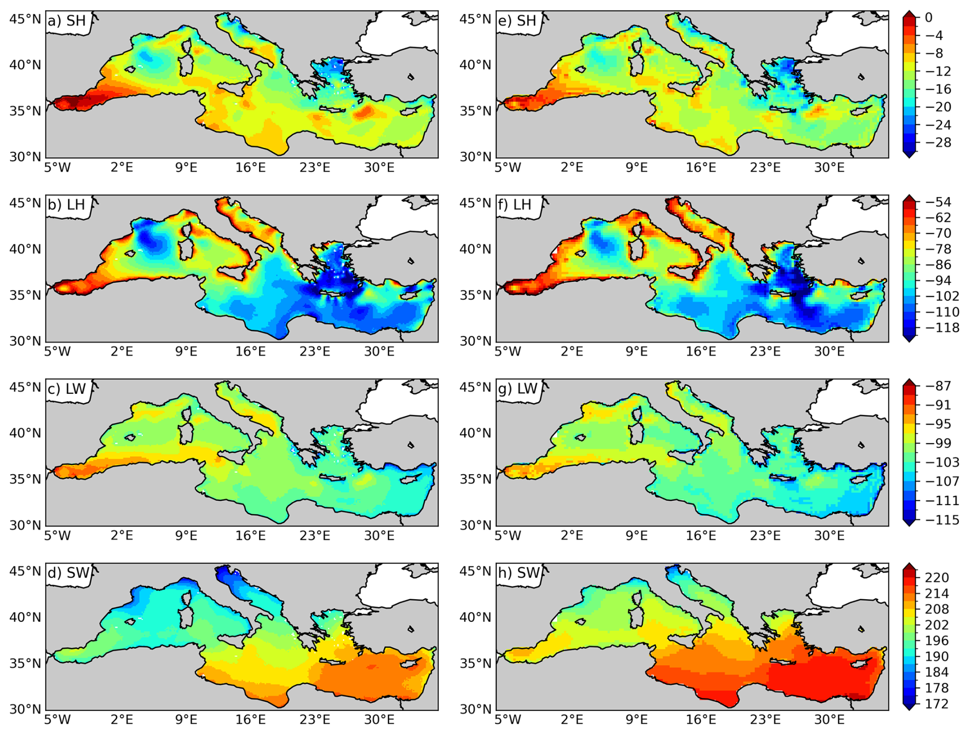
Figure 1 Annual means of heat flux components for the period of 2006–2020, computed from ECMWF (left panels) and ERA5 (right panels) daily time series. The corresponding ECMWF time series is shown in Supplement, Figs. S1 and S2.

Turbulent heat fluxes exhibit distinct sub-basin-scale patterns, varying between the eastern and western Mediterranean Seas as well as the Central Mediterranean region. The smallest mean sensible heat loss is observed in the whole Alboran sea area with absolute value range of 0–6 W m⁻², while the Aegean Sea and the centre of Gulf of Lion loses more heat in the maximum value of 25 W m⁻². Similarly, the highest absolute values of LH are recorded in the Gulf of Lion and the Aegean and Levantine Seas, attributed to the influence of strong and cold winds like the Mistral and Etesian in the north-western and eastern Mediterranean regions, respectively. The eastern Mediterranean emerges as the region with the highest evaporation, reaching approximately 122 W m⁻² in absolute value. Notably, along the south-eastern coastline, a wide range of maximum absolute values (102–122 W m⁻²) in the evaporation is observed. The turbulent heat fluxes show limited differences between the ECMWF and ERA5 datasets.

SW fields show the well-known meridional gradients with larger gradient values arising from the ECMWF dataset. The mean SW exhibits a gradual decline from the eastern to western Mediterranean, influenced by the variation of the solar zenith angle with longitudes. The first reason for SW differences between Western Mediterranean and Eastern Mediterranean is the latitudinal position of each sub-basin. Furthermore, SW differences using ECMWF and ERA5 datasets are connected to different cloud cover schemes (not shown), leading to a larger heat gain in the Eastern Mediterranean. Notably, the northern Adriatic region stands out with a distinct distribution, suggesting it receives relatively less annual solar radiation compared to other areas. In contrast, the mean longwave (LW) radiation distribution maintains a relatively consistent range of absolute values between 87–113 W m⁻² across the entire domain with absolute minimum values in the Alboran Sea, presumably due to the warm Atlantic surface water inflow. Overall, while the turbulent heat fluxes show limited differences between the ECMWF and ERA5 datasets, significant discrepancies are observed in radiative heat fluxes. Additionally, Fig. 1 shows the noisiness of the fluxes due to the ERA5 low resolution with respect to ECMWF while retaining an overall consistency.

Figure 2 shows seasonal variations in heat flux components for February and August using ECMWF data. Both SH and LH fluxes exhibit a greater spatial gradient in February compared to August. In winter, the SH loss is larger, especially in the Gulf of Lion, Aegean, and parts of the Adriatic, with stronger spatial gradients compared to summer. In August, SH flux becomes positive in the Aegean and the Alboran Sea. LH loss is highest in February in the whole eastern Mediterranean and the Gulf of Lion. In August, LH losses decrease in the western Mediterranean, with absolute value minima in the Alboran and Adriatic Sea, remaining largely negative in the lower part of in the Eastern Mediterranean. SW fields show the strongest seasonal cycle as expected, with the absolute maximum of 260–305 W m⁻² in summer and in the Eastern Mediterranean. LW is largest in absolute value in winter showing a small seasonal cycle. Significant seasonal variations are observed in the distribution range for radiative heat fluxes, low in February and high in August across the entire domain. These patterns are quite similar to the ones reported in the literature.

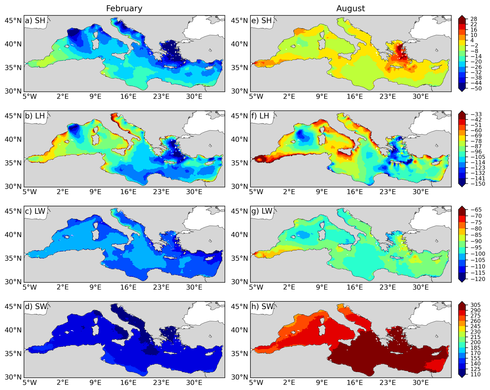
Figure 2 Seasonal variations of heat flux components: left column is the monthly average values for February and right column shows the average for August for the period 2006–2020 (ECMWF data).

3.2 Net heat budget estimation

The net surface heat flux Q_net is depicted in Fig. 3 for ERA5 and ECMWF and basin-average 15 year mean values are listed together with the literature in Table 1.

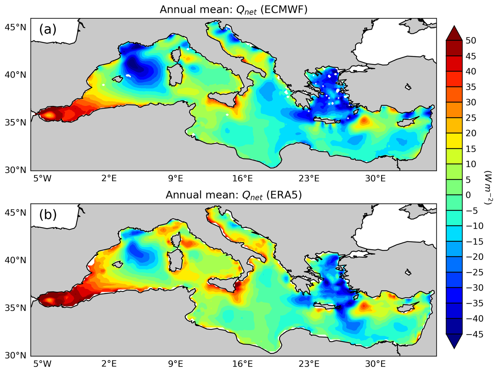
Figure 3 Comparison of the annual Q_net (W m⁻²) mean, computed from (a) ECMWF and (b) ERA-5 input datasets.

Table 1 Computed heat flux components and net heat fluxes (Q_net), and values from the references.

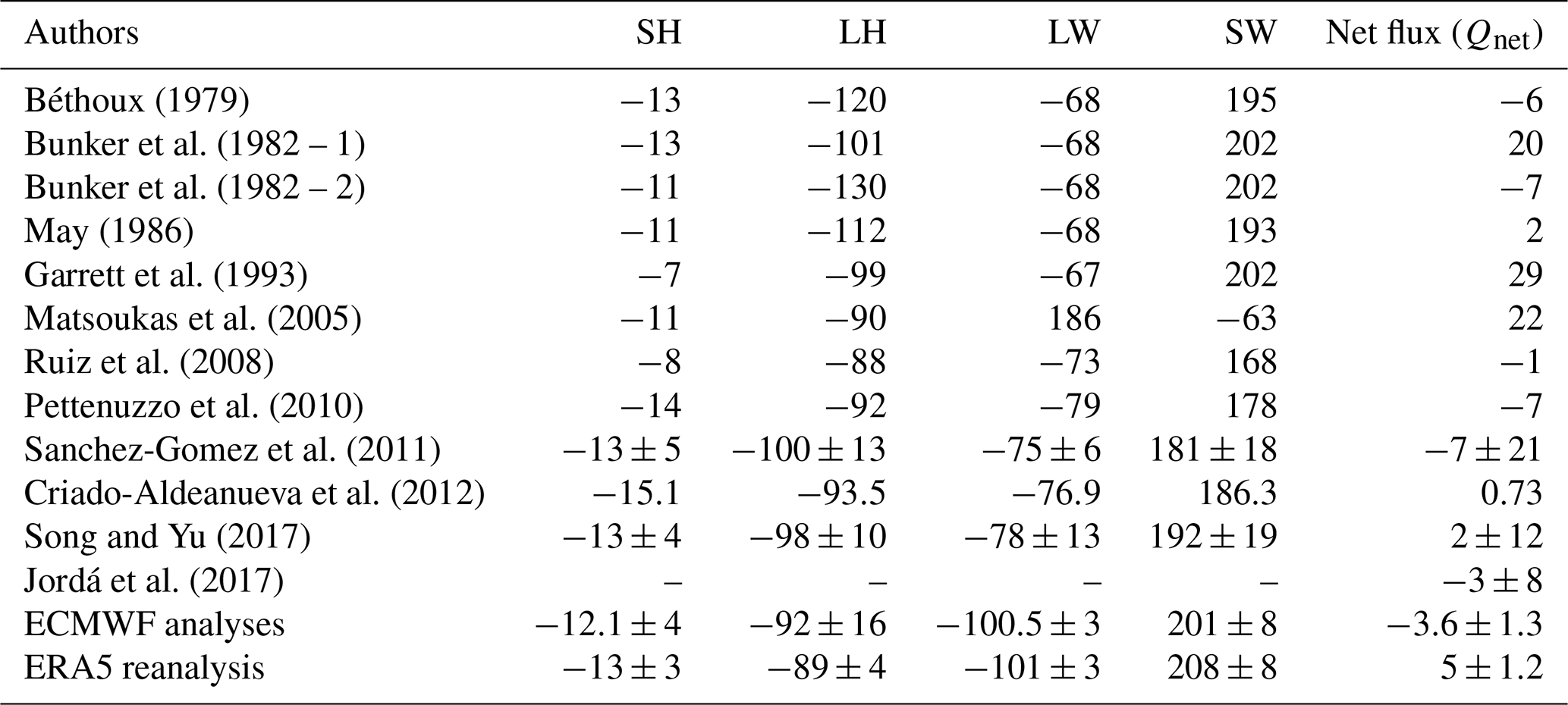
Figure 3 shows that the Gulf of Lion and the Aegean Sea are the areas of maximum heat losses while the basin gains heat in the Alboran Sea, in some areas of the Levantine basin, and in the shelf areas around the Italian peninsula.

The Mediterranean Sea gains comparatively more heat with the ERA5 inputs. Besides the difference in surface domain for Q_net, for both cases, air–sea flux dynamics is strongly visible in the Alboran Sea for net heat gain, in the Gulf of Lion for heat loss due to the continental cold wind (Mistral wind), and in the Aegean Sea due to the strong wind (Etesian wind) that blows during the summer period. Using ECMWF inputs, Q_net is −3.6 W m⁻², a value consistent with previous estimates for the Mediterranean Sea domain and for ERA5, it is 5 W m⁻² (Table 1). Errors in Q_net mean value are determined by a bootstrapping method where Q_net time series is resampled 5000 times to compute a standard deviation around the mean of the resampled time series (Tibshirani and Efron, 1993). We argue that our results show that the negative heat budget is achieved by using only ECMWF fields at high resolution, i.e. 0.125°. Higher resolution implies differences in all atmospheric fields used to compute the fluxes. Furthermore, ERA5 and ECMWF model physics and dynamics is different contributing to the differences in the mean heat budget. However, both datasets use observations, and we argue that the most relevant difference between the analysis and the reanalysis data set is the resolution due to the peculiar geometry of the Mediterranean Sea.

Since all the datasets used in the literature are coarser, this is most likely the reason of the failure to determine the correct heat budget closure value. In Pettenuzzo et al. (2010) several ad-hoc corrections were made to the surface atmospheric fields to obtain the negative heat flux budget while in Sanchez-Gomez et al. (2011) they used an ensemble of deterministically downscaled ERA40 fluxes giving rise to a very large uncertainty. Considering a recent literature, our resulted Q_net is closely matched with the computed net heat budget of $-\mathrm{3}\pm \mathrm{8}$ W m⁻² from Jordá et al. (2017), but their result was associated to large temporal uncertainties from the surface fluxes through Gibraltar Strait.

Spatially, the mean Q_net distribution generally shows a heat loss across much of the Eastern Mediterranean. Overall, distributions of more positive net heat budget values for the western Mediterranean and negative for the eastern Mediterranean have matched with the similar result from Criado-Aldeanueva et al. (2012). Strong spatial gradients are evident, particularly in the Aegean Sea, although a few patches displaying net heat loss (negative Q_net) are also noticeable in this vicinity. Conversely, the western Mediterranean exhibits a stronger heat gain area, which appears particularly concentrated zone in the Gulf of Lion region and this feature is apparent in results from both atmospheric datasets. Such a spatial related uncertainty in Q_net represents a significant challenge for accurately closing regional heat budgets as well as validating existing ocean circulation models within the complex Mediterranean basin.

4 Probability distributions of the turbulent heat fluxes

In this section, we analyse the probability distribution of turbulent heat fluxes computed using ECMWF data set only and for the anomaly heat fluxes. Recent studies by Gulev and Belyaev (2012) and Korolev et al. (2015) have analysed the statistical distributions of turbulent heat fluxes, and their findings are used here for comparison. Radiative flux components are excluded from this analysis, as they do not exhibit extremes of comparable magnitude to those of turbulent fluxes (Fig. S3). This suggests low skewness and kurtosis in their distributions, reducing the relevance of a detailed probability density function analysis for these components.

If we indicate the time series of each component of the heat budget with X_n we can define the heat flux climatology as:

$$\begin{array}{}\text{(12)}& Q_t={\displaystyle \frac{\mathrm{1}}{n}}\sum _{j=\mathrm{1}}^n{X}_{tj}\end{array}$$

where “t” indicates the day of the year, and “j” is the number of years. The anomaly time series is computed by subtracting the long-term seasonal climatology Q_t from the observed heat flux time series X_tj and it will be indicated by:

$$\begin{array}{}\text{(13)}& {\stackrel{\mathrm{̃}}{X}}_{tj}=X_{tj}-Q_t.\end{array}$$

4.1 SH flux distribution

We found that gaussian or skew-normal distributions are not well fit for SH flux, as evident from the histograms at single grid points shown in Fig. 4a. The histograms reveal a singularity around zero, indicating that the skew-normal distribution may not adequately capture the distribution of these values. This observation is consistent with findings by Gulev and Belyaev (2012), and we provide further explanation in the Appendix A.

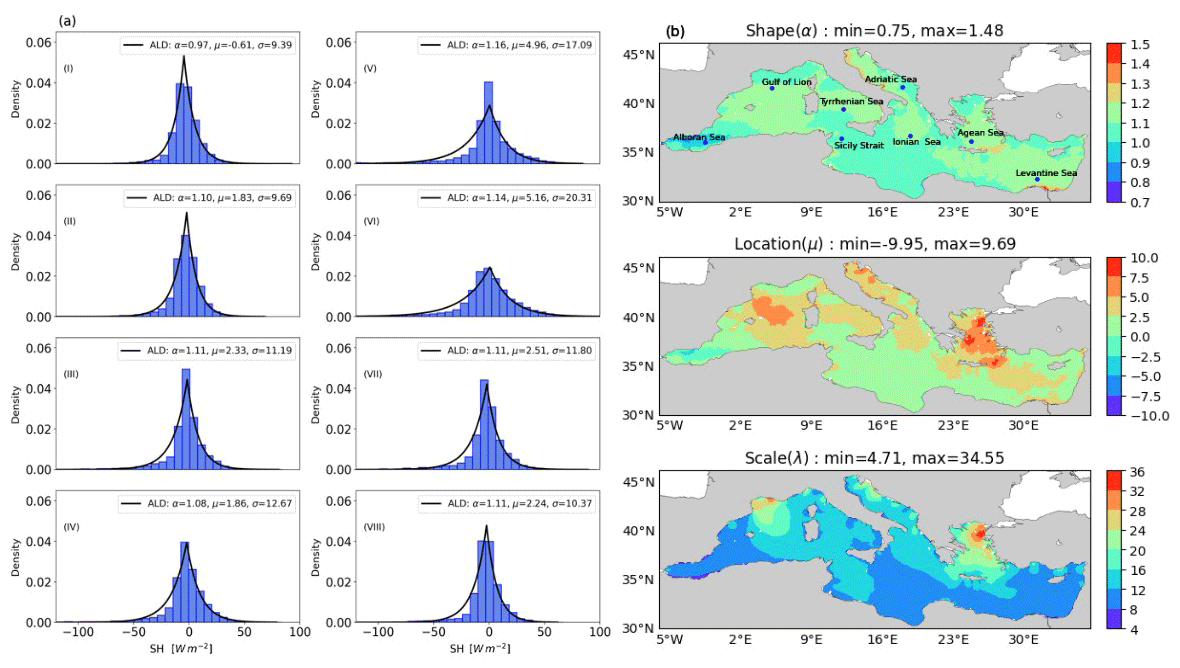
Figure 4 (a) The single grid point histograms for SH flux anomalies from the eight sampling locations for the period of 2006–2020, (b) the Asymmetric Laplace PDF parameter (α, μ, λ) distributions from computed SH flux anomaly for the observation period. Sampling points: (I) Alboran Sea, (II) Gulf of Lion, (III) Tyrrhenian Sea, (IV) Sicily Strait, (V) Adriatic Sea, (VI) Ionian Sea, (VII) Aegean Sea, (VIII) Levantine Sea.

The most common distribution with such near-discontinuous behaviour at the origin is the three-parameter Asymmetric Laplace Distribution (ALD) (Yu and Zhang, 2005) that we can defined as

$$\begin{array}{}\text{(14)}& F(x,\mathit{\alpha }\mathit{\mu },\mathit{\lambda })={\displaystyle \frac{\mathit{\lambda }}{\mathit{\alpha }+\frac{\mathrm{1}}{\mathit{\alpha }}}}\left\{\begin{array}{ll}\exp (\mathit{\lambda }/\mathit{\alpha }(x-\mathit{\mu }\left)\right)& \mathrm{if}x<\mathit{\mu }\\ \exp (-\mathit{\lambda }\mathit{\alpha }(x-\mathit{\mu }\left)\right)& \mathrm{if}x\ge \mathit{\mu }\end{array}\right.\end{array}$$

where x is the random variable time series, α is the shape parameter, μ is the location and λ the scale.

From the single grid point histogram, we have observed a one or two sharp peaks in the distribution that matches well with the Asymmetric Laplace Distribution (ALD) PDF. In accordance with findings by Yu and Zhang (2005), the distribution of the sensible heat (SH) flux anomaly time series exhibits characteristics of a double exponential distribution. This is evident from the histograms displaying both positive and negative skewness with long tails, as depicted in Fig. 4a. The ALD parameters for the SH flux anomaly time series are illustrated in Fig. 4b. The shape parameter (α) falls within the positive range of 0.73 to 1.48, indicating a moderate to high degree of peakiness in the distribution. Additionally, the location parameter (μ) exhibits mostly positive values while a small area in the Alboran Sea shows negative values, suggesting a shift in the central tendency of the distribution. Notably, the scale parameter (λ) displays a similar structure to the SH flux climatology depicted in Fig. 1.

To check the quality of the fit, moments of both applied and theoretical PDF are compared (presented in Fig. S4). The comparison shows the estimations of the three moments in the left panel for the observed SH flux and right panel for ALD PDF parameters. It can be seen that variances and skewness are similar in distribution while kurtosis differ at noticeable range. This observation is likely attributed to the fact that the kurtosis for the asymmetric Laplace distribution remains constant regardless of changes in the scale parameter.

4.2 LH flux distribution

In the case of the LH flux, no sharp exponential peaks were observed; instead, large skewness and long tails were identified. Therefore, we applied the skew-normal PDF which is defined by α(∈R) as the shape parameter, μ(∈R) the location parameter, and λ>0 the scale parameter (Azzalini, 1985) and defined as:

$$\begin{array}{}\text{(15)}& f(x,\mathit{\alpha },\mathit{\mu },\mathit{\lambda })={\displaystyle \frac{\mathrm{2}}{\mathit{\lambda }}}\mathit{\varphi }\left({\displaystyle \frac{x-\mathit{\mu }}{\mathit{\lambda }}}\right)\mathrm{\Phi }\left(\mathit{\alpha }\left({\displaystyle \frac{x-\mathit{\mu }}{\mathit{\lambda }}}\right)\right)\end{array}$$

where,

$$\begin{array}{}\text{(16)}& {\displaystyle }& {\displaystyle }\mathit{\varphi }\left({\displaystyle \frac{x-\mathit{\mu }}{\mathit{\lambda }}}\right)={\displaystyle \frac{\mathrm{1}}{\sqrt{\mathrm{2}\mathit{\pi }}}}{e}^{-\frac{\mathrm{1}}{\mathrm{2}}\frac{(x-\mathit{\mu }{)}^{\mathrm{2}}}{{\mathit{\lambda }}^{\mathrm{2}}}}\text{(17)}& {\displaystyle }& {\displaystyle }\mathrm{\Phi }\left(\mathit{\alpha }\left({\displaystyle \frac{x-\mathit{\mu }}{\mathit{\lambda }}}\right)\right)=\underset{-\mathrm{\infty }}{\overset{\mathit{\alpha }\left(\frac{x-\mathit{\mu }}{\mathit{\lambda }}\right)}{\int }}\mathit{\varphi }\left(t\right)\mathrm{d}t.\end{array}$$

A skew-normal PDF is an extension of the normal distribution while covering the skewness and containing the general characteristics of a Gaussian distribution (Flecher et al., 2010).

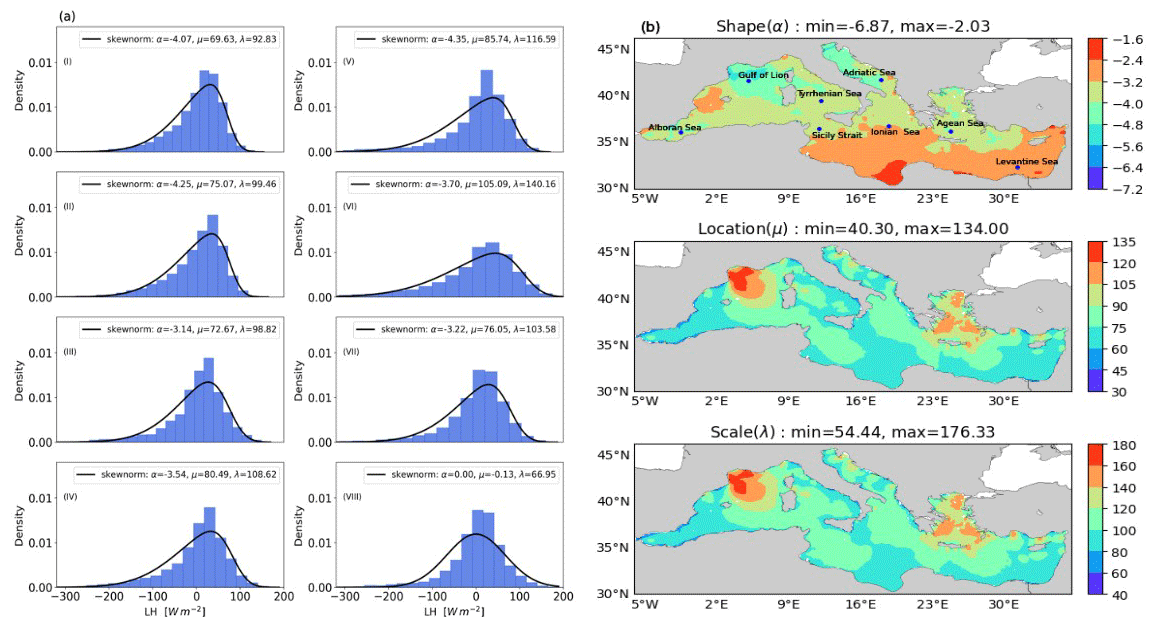
Figure 5 (a) The single grid point histograms for LH flux anomalies at the eight sampling locations for the period of 2006002020, (b) the skew-normal PDF parameter (α, μ, λ) distributions for computed LH flux anomaly for the observation period – sampling points: (I) Alboran Sea, (II) Gulf of Lion, (III) Tyrrhenian Sea, (IV) Sicily Strait, (V) Adriatic Sea, (VI) Ionian Sea, (VII) Aegean Sea, (VIII) Levantine Sea.

To examine visually the quality of PDF fit on LH flux anomaly values, histograms from eight sea locations were fitted with the skew-normal PDF, as shown in Fig. 5a. Figure 5b displays the parameter spatial variability. The shape parameter distribution ranges from −6.83 to −2.5, with negative values observed across all points. This spatial distribution of α, exhibiting a negative range, aligns with the negatively skewed pattern identified in the single grid point PDF fitting test. Furthermore, the spatial distribution structure of the location and scale parameters demonstrates a positive correlation across most locations.

In the Supplementary material, a comparison of statistical moments is conducted to qualitatively validate the fit (Fig. S5). There is notable agreement in the variance distributions between the observed LH flux anomaly and skew-normal PDF. While the skewness distributions mismatch at negligible level, with the theoretical PDF skewness predominantly ranging from −0.9 to −0.3, whereas the observed skewness exhibits a variation range spanning from −1.2 to over −0.3. Lastly, the kurtosis distribution of the skew-normal PDF differs in the Aegean Sea, Alboran Sea and Gulf of Lion area.

4.3 Evaluation of the PDF fitting

In this section, we conducted a goodness of fit test to measure the distance between the empirical distributions and the fitted ones. The objective of this evaluation test was to assess the degree of agreement between the applied theoretical distribution and the observed time series. The χ² method, a well-accepted test, was employed to measure the distance between two independent distributions.

We compared the results of the chi-squared test for the turbulent heat fluxes computed using the ECMWF and ERA5 datasets. The decision rule for the χ² test was determined based on the level of significance, set at 0.05, and the degrees of freedom, defined as $\mathrm{DF}=N-\mathrm{np}$, where N represents the number of empirical histogram bins and np is the number of distribution parameters (i.e., 3 for both the ALD and skew-normal distributions). In the supplementary material we show the maps of χ² test statistics (Fig. S6). The chi-squared results for the SH and LH fluxes computed using the ECMWF dataset indicate that almost all surface grid points are well-fitted with the applied theoretical PDFs. With the critical threshold of 33.92 (Elderton, 1902) for P values, we observed a very few mismatches, mainly located near the coasts.

5 How do heat loss extremes contribute to the heat budget closure hypothesis?

The heat budget closure problem is associated with achieving a net negative heat flux, as discussed before. We test here the hypothesis that the negative long term mean negative heat budget of Table 1 for ECMWF data is correlated to the extremes in heat losses during autumn–winter.

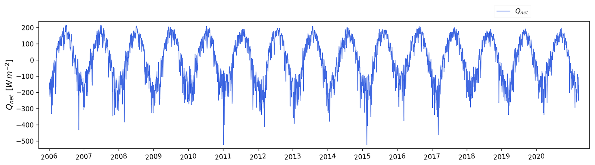
Figure 6 Basin averaged time series of the computed daily Q_net (units W m⁻²) from the ECMWF computed heat fluxes, for the period 2006–2020.

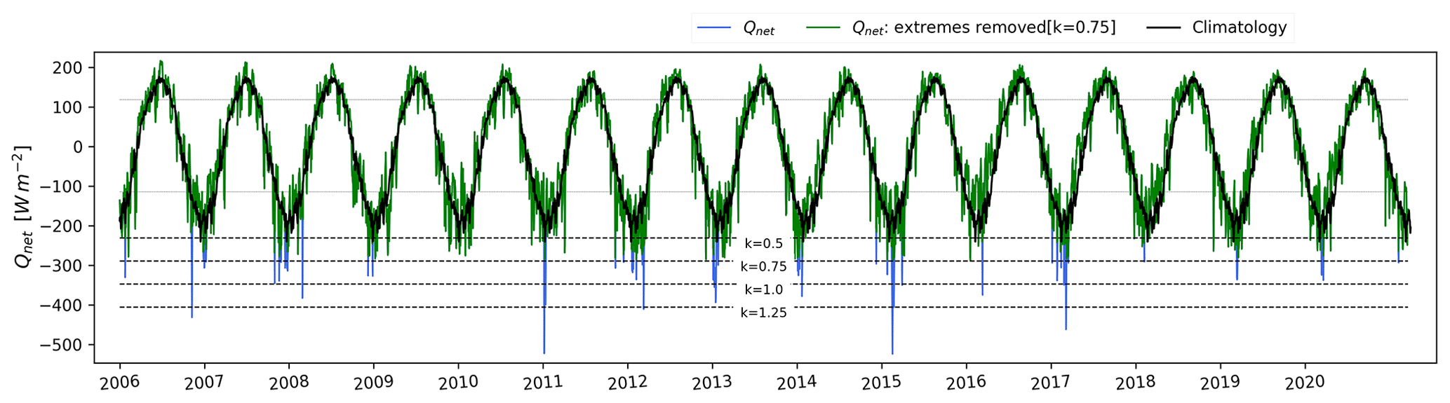
Figure 7 Time series of the basin averaged Q_net mean, Q_net extremes removed mean, and long-term yearly climatology and four lower quantile boundary line marked with dashed lines using different k values [k=1.25, 1, 0.75, 0.5].

Figure 6 illustrates the Q_net basin average daily time series, revealing a value range varying between 200 and −500 W m⁻². Notably, the most pronounced extreme negative heat losses, reaching up to −500 W m⁻² occur in the winters of 2011, 2015 and 2017. They approximately coincide with western Mediterranean Deep Water formation events, as documented in Escudier et al. (2021). To identify and remove the potential extremes in our computed Q_net time series, we apply the Interquartile Range (IQR) method which measures the spread of a dataset and calculate the difference between the third quartile (Q₃) and the first quartile (Q₁). The IQR threshold is computed by the difference between the 1st quartile (Q₁) and 3rd quartile (Q₃) of the observed dataset:

$$\begin{array}{}\text{(18)}& {\displaystyle }& {\displaystyle }\mathrm{IQR}=Q_{\mathrm{3}}-Q_{\mathrm{1}}\text{(19)}& {\displaystyle }& {\displaystyle }\mathrm{Threshold}=Q_{\mathrm{1}}-k\cdot \mathrm{IQR}.\end{array}$$

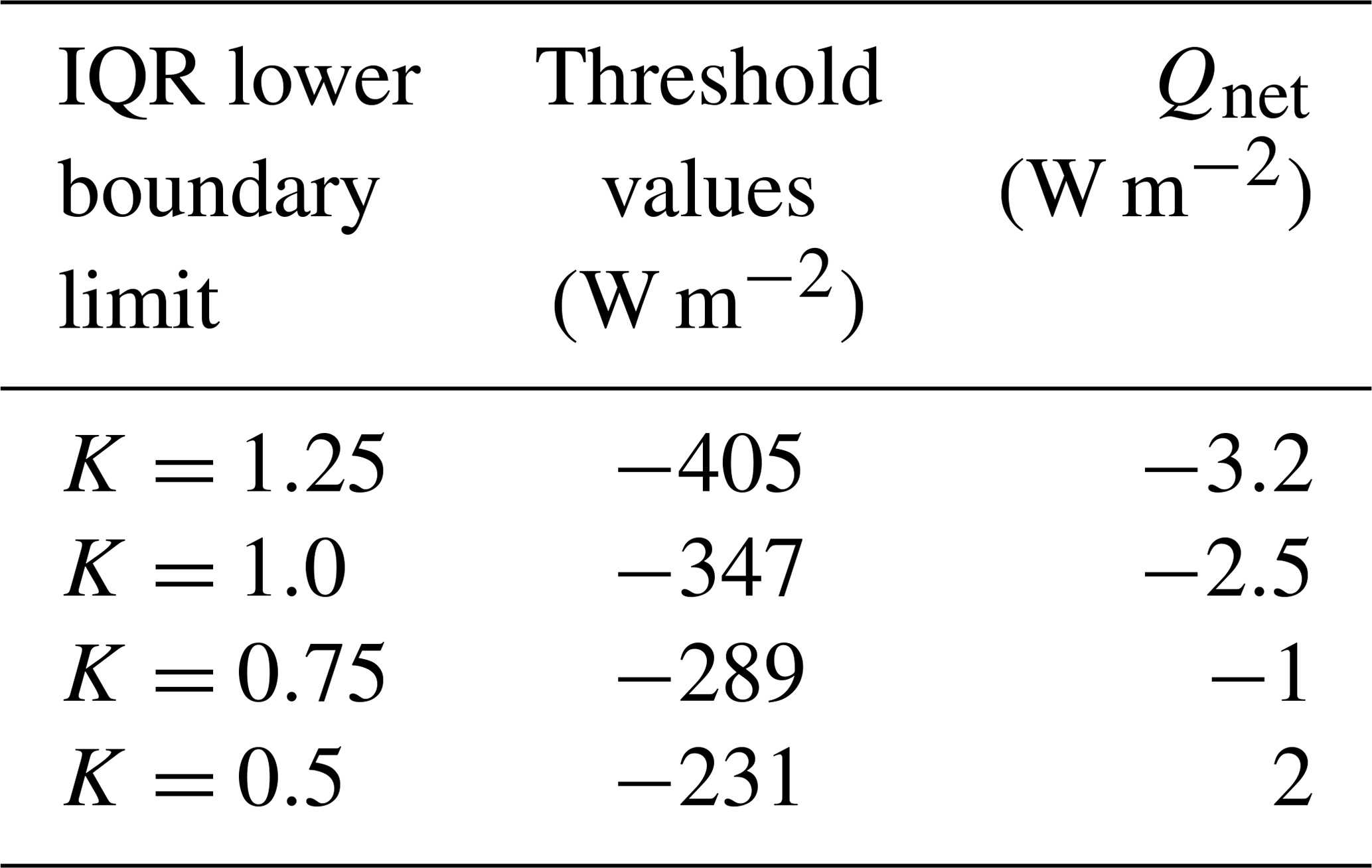
We used different values for k to exclude the negative extremes, which correspond to the largest heat losses. These extreme values were replaced with long-term daily climatological values (computed using Eq. 11) and the long term mean neat heat budget Q_net is recomputed.

The resulting Q_net for different thresholds is displayed in Table 2 and the thresholds are shown in Fig. 7 together with the daily climatology. If compared with the long term mean heat budget in Table 1 ($-\mathrm{3.6}\pm \mathrm{1.3}$ W m⁻²), we see that eliminating the winter extremes produces a smaller long term mean heat loss up to changing the sign to positive values. We argue that the ECMWF net negative heat extremes determine the ECMWF negative long term mean heat budget. Furthermore, if we calculate the yearly mean value of the seasonal climatology, we obtain the value of +4 W m⁻², which confirms again the importance of extremes in the heat budget closure of the Mediterranean Sea.

Table 2 Different lower quantile boundary limits used to replace potential extremes and the resulting long-term mean basin averaged Q_net values.

The Q_net could become an impact indicator of the Mediterranean for sea level trends in the basin. The net heat budget in fact relates to the sea level tendency (Pinardi et al., 2014) in the Mediterranean Sea and could be considered as a key indicator of climate impacts in the Mediterranean Sea.

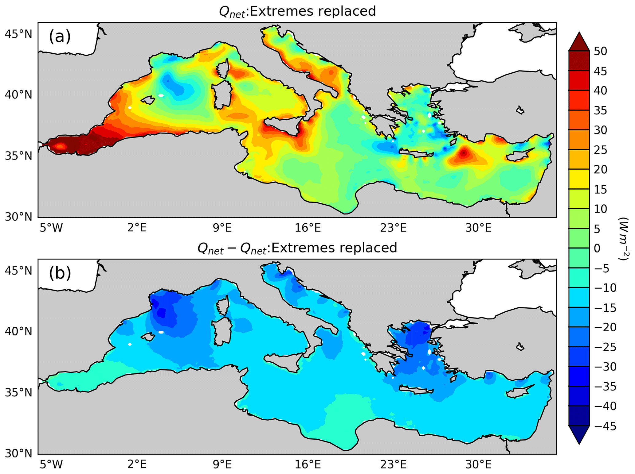
Figure 8 (a) Long term mean net heat flux after the removal of extremes (Q_net: extremes replaced) using threshold of −289 W m⁻² (K=0.75). (b) The time mean distribution computed from the difference between Q_net (Fig. 3a) and “Q_net: extremes replaced” time series. It shows a significant reduction of heat losses in the Gulf of Lion, Adriatic Sea and Aegean Sea regions.

Figure 8 presents the new long-term mean spatial distribution of the surface heat budget after removing negative extreme values using a threshold of −289 W m⁻² (K=0.75). The figure illustrates that these extreme events exert a substantial influence on the overall structure of the net heat budget in the Mediterranean Sea, with particularly pronounced effects in the Gulf of Lion, the Aegean Sea, the eastern Adriatic Sea, and along the southern Turkish shelves.

6 Discussion and conclusions

The primary objective of this investigation is to revisit the heat budget closure hypothesis from atmospheric consolidated data sets that are nowadays used frequently to drive ocean models. Simultaneously, we intend to model the statistical distributions of turbulent heat fluxes and assess the contribution of extremes into the net heat budget closure of the Mediterranean Sea. For this analysis, we covered a 15-year period from 2006 to 2020 with a daily time series frequency. The reason for the choice of this time range is that ECMWF analyses became quite stable starting from 2006 while before the model was at coarse resolution, like ERA5's model. Our strategy is to use the same SST and the same bulk formula but different atmospheric reanalysis and analysis surface variable data sets and compare the value of the long term mean heat budget in the Mediterranean Sea.

Firstly, the surface heat budget of the Mediterranean Sea was analysed to examine average annual mean and seasonal variations. The largest component of the heat budget is the net solar radiation (SW), followed by the latent heat (LH), longwave radiation (LW), and then sensible heat (SH), as shown in the literature (Table 1). All heat flux components exhibit significant seasonality, as illustrated in Fig. 2. Differences appear in the structure of the fluxes, especially the SW and LW, when different atmospheric data sets are used, a conclusion aligning with a suggestion from Marullo et al. (2021) on the sensitivity of LW estimates from the atmospheric dataset used to calculate fluxes. We compared the ERA5-derived surface radiative fluxes with the computed ERA5 heat fluxes presented in Fig. 3b and found that the ERA5 longwave (LW) fluxes are substantially overestimated in absolute magnitude (Fig. S7). The associated uncertainty is comparable in order of magnitude to that reported by Marullo et al. (2021), who analysed an observational dataset at a specific site. Nonetheless, compensating biases between the SW and LW components (Fig. S8) result in a net radiative heat balance difference between ERA5-derived and computed heat fluxes that is large primarily in the southern Mediterranean, where ERA5-derived exhibits reduced LW flux values.

The basin-average net heat flux, Q_net, was calculated to be $-\mathrm{3.6}\pm \mathrm{1.3}$ W m⁻² for ECMWF analysis data while it is 5±1.2 W m⁻² for ERA5 (Table 1). This finding supports the conclusion that heat budget closure hypothesis cannot be satisfied with a relatively coarse reanalysis atmospheric data set. Our initial question was: is the Mediterranean Sea in the past 15 years still losing heat at the surface? The answer is yes if we use a high-resolution ECMWF atmospheric analysis. Additionally, comparing the Q_net estimates derived from ERA5 and ECMWF with the same bulk formulas demonstrates that the uncertainty peaks in the atmospheric forcing resolution and possibly cloud cover, the latter affecting the radiative components of the heat budget.

Furthermore, we have demonstrated that the probability density of surface heat fluxes can be modelled and fitted with a three-parameter PDF composed of a shape, a location, and a scale parameter. All the turbulent heat flux components show asymmetric behaviour. There is encouraging agreement between the first two statistical moments of the fitted PDF and the observed values. Kurtosis does not seem to be properly captured by the PDF used but our time series is too short to arrive at a definitive conclusion. For the SH we demonstrate that the Asymmetric Laplace Distribution PDF is generated by the contributing distributions of wind speed (Weibull) and temperature difference Skew Normal). We believe this is the first time that such kind of relationship is demonstrated.

Gulev and Belyaev (2012) applied the two-parameter Fisher–Tippett distribution (also known as the Gumbel distribution) to monthly sensible and latent heat fluxes derived from NCEP–NCAR reanalysis fields. Their approach focused on using the mean and standard deviation to estimate the distribution's location and scale parameters relevant to extreme events. However, the Gumbel distribution has a fixed skewness, limiting its ability to capture the contribution of rare, asymmetric extremes. In contrast, our study analysis anomalies from the seasonal cycle using full probability distributions that allow for variable skewness. This better reflects the nature of atmospheric and oceanic variables, which are often inherently skewed (Sardeshmukh and Penland, 2015), and is essential for understanding the influence of extremes on the surface heat budget. Our findings show that incorporating a shape parameter is key to accurately capturing distribution structure and preserving asymmetric tails. This analysis provides a useful framework for validating surface flux products and assessing their variability, particularly important given that surface fluxes are the dominant source of uncertainty in the Mediterranean net heat balance (Jordá et al., 2017). Correctly estimating skewness is crucial, as a small number of extreme outliers, especially during intense winter events, can disproportionately affect the basin-wide mean and determine whether heat budget closure is achieved.

For the first time, we have investigated the effects of extreme heat losses in the Mediterranean Sea in the long term mean basin averaged heat budget. The northern basin areas are the site of the largest heat losses (Gulf of Lion and the Aegean Sea, Adriatic Sea and the Turkish southern coasts). Exclusion of the negative extremes in these areas resulted in a change in the sign of long term mean heat loss. The anomaly threshold value (−231 W m⁻², Table 2) resulted a long-term positive net heat flux, which is inconsistent with the basin's heat flux closure hypothesis. Our second initial question was: what is the cause of the Mediterranean Sea negative long-term mean heat budget? The answer is that the long-term mean, basin averaged heat loss is due to winter extremes in the Northern regions of the Mediterranean Sea.

In conclusion, understanding the characteristics and distributions of air–sea heat fluxes are crucial for gaining insights into variations in the heat budget. Furthermore, the PDF analysis of turbulent heat fluxes will allow us to have a better understanding of the extreme events and their contributions to the net negative heat budget. The next steps could involve a machine learning study of air–sea flux bulk parametrizations for different atmospheric data sets and coupled models, using as target the heat flux data set from this study.

Appendix A

Here, we show that the characteristics of the SH flux distribution are due to the specific form of the heat flux as given by Eq. (10), i.e. a multiplication of two distributions, wind speed, Q(v), known to be a Weibull, and temperature differences, R(DT), taken to be a Skew Normal.

Let us indicate with P(v⋅DT) the combined SH distribution of Q(v) and R(DT) the temperature difference as in Eq. (9). Assuming that the two distributions are independent, the combined distribution is the product of Q and R. If we now define the variable $z=v\cdot \mathrm{DT}$, the new combined distribution on the heat flux variable z is given by the Mellin transform and convolution, described in Papoulis and Pillai (2002). The resulting P distribution is an Asymmetric Laplace Distribution (ALD) like distribution which is similar to the one computed in Fig. 4.

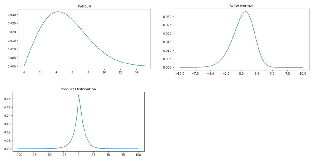
Figure A1 Histograms presenting the two original distributions, Q(v) (upper left quadrant, units wind speed) and R(DT) (upper right quadrant, units °C) and the combined distribution for SH flux in units of W m⁻². The parameters used for the two original distributions are: k=2.0 for the Weibull shape, λ=6.0 for the Weibull scale; $\mathit{\alpha }=-\mathrm{2.0}$ for the Skew Normal shape, μ=2.0 for the Skew Normal location and ω=2.5 for the Skew Normal scale.

Appendix B

The statistical moments for the skew-normal PDF are given by:

$$\begin{array}{}\text{(B1)}& {\displaystyle }& {\displaystyle }E\left(x\right)=\mathit{\mu }+\mathit{\lambda }\mathit{\delta }\sqrt{{\displaystyle \frac{\mathrm{2}}{\mathit{\pi }}}}\text{(B2)}& {\displaystyle }& {\displaystyle }{\mathit{\sigma }}^{\mathrm{2}}={\mathit{\lambda }}^{\mathrm{2}}\left(\mathrm{1}-{\displaystyle \frac{\mathrm{2}{\mathit{\delta }}^{\mathrm{2}}}{\mathit{\pi }}}\right)\text{(B3)}& {\displaystyle }& {\displaystyle }{\mathit{\mu }}_{\mathrm{3}}=(\mathrm{4}-\mathit{\pi }){\displaystyle \frac{(\mathit{\delta }\cdot \sqrt{\mathrm{2}}/\mathit{\pi }{)}^{\mathrm{3}}}{\mathrm{2}{\left(\mathrm{1}-\mathrm{2}{\mathit{\delta }}^{\mathrm{2}}/\mathit{\pi }\right)}^{\mathrm{3}/\mathrm{2}}}}\text{(B4)}& {\displaystyle }& {\displaystyle }{\mathit{\mu }}_{\mathrm{4}}=\mathrm{2}(\mathit{\pi }-\mathrm{3}){\displaystyle \frac{{\left(\mathit{\delta }\sqrt{\frac{\mathrm{2}}{\mathit{\pi }}}\right)}^{\mathrm{4}}}{{\left(\mathrm{1}-\frac{\mathrm{2}{\mathit{\delta }}^{\mathrm{2}}}{\mathit{\pi }}\right)}^{\mathrm{2}}}}\end{array}$$

where $\mathit{\delta }=\frac{\mathit{\alpha }}{\sqrt{\mathrm{1}+{\mathit{\alpha }}^{\mathrm{2}}}}$. Since the expected value, E, of the time series is zero, we deduce that:

$$\begin{array}{}\text{(B5)}& \mathit{\mu }=-\mathit{\lambda }\mathit{\delta }\sqrt{{\displaystyle \frac{\mathrm{2}}{\mathit{\pi }}}}.\end{array}$$

In other words, location and shape parameters have opposite signs since the scale parameter, λ, is always positive.

SH flux anomaly distribution was analysed with the Asymmetric Laplace Distribution PDF, its statistical moments given by:

$$\begin{array}{}\text{(B6)}& {\displaystyle }& {\displaystyle }\mathrm{mean}=\mathit{\mu }+{\displaystyle \frac{\mathrm{1}-{\mathit{\alpha }}^{\mathrm{2}}}{\mathit{\lambda }\mathit{\alpha }}}\text{(B7)}& {\displaystyle }& {\displaystyle }\mathrm{variance}={\displaystyle \frac{\mathrm{1}+a^{\mathrm{2}}}{{\mathit{\lambda }}^{\mathrm{2}}{\mathit{\alpha }}^{\mathrm{2}}}}\text{(B8)}& {\displaystyle }& {\displaystyle }\mathrm{Skewness}={\displaystyle \frac{\mathrm{2}\left(\mathrm{1}-{\mathit{\alpha }}^{\mathrm{6}}\right)}{{\left({\mathit{\alpha }}^{\mathrm{4}}+\mathrm{1}\right)}^{\frac{\mathrm{3}}{\mathrm{2}}}}}\text{(B9)}& {\displaystyle }& {\displaystyle }\mathrm{Kurtosis}={\displaystyle \frac{\mathrm{6}\left(\mathrm{1}+{\mathit{\alpha }}^{\mathrm{3}}\right)}{{\left(\mathrm{1}+{\mathit{\alpha }}^{\mathrm{4}}\right)}^{\mathrm{2}}}}.\end{array}$$