Rogue wave indicators from global models and buoy data

Rogue waves pose substantial risks to maritime operations and offshore infrastructure, yet their formation mechanisms and predictability remain poorly understood. This study analyses real rogue wave occurrences using in situ observations from CDIP wave buoys from the Free Ocean Wave Data (FOWD) dataset and model-based estimates from ERA5 reanalysis and the ECMWF CY47R1 high-resolution hindcast. Seasonal distributions, wave height comparisons, and spectral analyses reveal that models systematically underestimate extreme wave events due to spectral smoothing and spatial averaging. A key finding is that rogue waves are usually preceded by a sharp decrease in crest-trough correlation below 0.5, followed by a rapid increase usually above 0.6, indicating a transition to a more structured wave field. This pattern, accompanied by spectral bandwidth narrowing and increased relative energy in the 0.25–1.5 Hz range, suggests energy focusing mechanisms play a critical role. Analysis of rogue wave events at four CDIP buoy stations show that the crest-trough correlation parameter alone is not a good rogue wave indicator, but its temporal variability is. These results highlight the need for improved modelling by integrating dynamic wave field specific parameters and high-resolution numerical models to enhance rogue wave risk assessments on a global scale.

1 Introduction

Rogue waves, also known as freak waves, represent one of the most enigmatic and dangerous phenomena in oceanography. These waves, characterized by their exceptional height relative to the surrounding sea state, pose significant threats to maritime safety, including risks to vessels, offshore infrastructure, and coastal regions (Bitner-Gregersen et al., 2015;; Kharif et al., 2009; Didenkulova, 2020; Didenkulova et al., 2023). Tradionally defined as waves with a maximum height (H_max) exceeding twice the significant wave height (H_s), rogue waves have been documented across diverse oceanic environments, from deep waters to nearshore zones (Dysthe et al., 2008; Toffoli et al., 2005). In this study the common criterion $H_{\max }/H_{\mathrm{s}}$ > 2.0 is adopted; some studies may use ∼ 2.2×H_s or a crest threshold. The global significance of rogue waves was underscored by the observation of the New Year's Wave at the Draupner oil rig in 1995, which triggered a renaissance in their scientific study (Haver, 2003; Adcock et al., 2011).

Over the past two decades, various physical mechanisms have been proposed to explain the occurrence of rogue waves. These include nonlinear processes such as modulation instability (Benjamin-Feir instability), wave focusing through dispersion, and interactions with bathymetric features (Cattrell et al., 2018; Fedele et al., 2016; Gramstad et al., 2018a). Analytical models, numerical simulations, and laboratory experiments have provided significant insights into these mechanisms (Onorato et al., 2005; Onorato et al., 2003; Toffoli et al., 2011). However, the real-world application of these theories remains limited due to the rarity of rogue wave events and the sparse availability of in-situ observations (Azevedo et al., 2022; Baschek and Imai, 2011; Barbariol et al., 2019b). This scarcity of high-quality observational data, particularly from buoys, has constrained the development of robust predictive models (Orzech and Wang, 2020). From a scientific perspective, rogue waves challenge conventional understanding of ocean dynamics.

Recent advancements in reanalysis datasets and wave modeling offer a promising avenue for addressing these limitations. Reanalysis products such as ERA5 and higher-resolution models like ECMWF's CY47R1 provide global coverage of wave parameters, integrating observational and modeled data to simulate historical ocean conditions. While ERA5 assimilates observational data and is designed to reflect real-world conditions, its spatial resolution (approximately 40 km) can result in the smoothing of extremes (ECMWF, 2021; Hersbach et al., 2020; Barbariol et al., 2019a). In contrast, the CY47R1 wave model, with its higher resolution (18 km) and enhanced spectral fidelity, is potentially more sensitive to localized, transient events such as rogue waves, albeit without assimilating observational wave data (Cavaleri et al., 2022; ECMWF, 1979–1989, 1990–1999, 2000–2009, 2010–2020; Lobeto et al., 2024). In phase-averaged models, higher resolution does not resolve individual crests; but it improves representation of envelope statistics and gradients (e.g., distributions of H_s and envelope-based 〈H_max〉). It is important to stress that phase-averaged spectral wave models cannot explicitly capture rogue waves, meaning that they do not simulate individual wave realizations or isolated extreme crests in time and space; rather, they describe the wave field statistically via spectral moments and probabilistic envelope-based estimates that characterize the likelihood of extremes within a given window.

While traditional theories of formation have emphasized nonlinear modulational instability (Teutsch and Weisse, 2023; Onorato et al., 2009), recent studies highlight the role of spectral energy distribution, wave group dynamics, and crest-trough correlation in governing rogue wave emergence (Hafner et al., 2021b; Gemmrich and Cicon, 2022; Gemmrich and Thomson, 2017; Cicon et al., 2024). Given the severe implications of these waves for navigation, offshore energy production, and climate-driven wave climate shifts, there is a growing need for improved methodologies that detect and predict rogue wave conditions using this new knowledge.

Numerous studies have investigated the mechanisms underlying rogue wave formation (Babanin and Rogers, 2014; Bennett et al., 2012; Onorato et al., 2009; Gemmrich and Cicon, 2022). Early research primarily focused on the role of modulational instability, which predicts that under specific conditions, wave groups can undergo nonlinear focusing, leading to extreme wave growth (Adcock et al., 2015; Janssen, 2003; Horikawa and Maruo, 1988; Donelan and Magnusson, 2005). However, observational evidence suggests that rogue waves also frequently occur in environments where modulational instability is weak or absent, particularly in wind-sea dominated conditions (Fedele et al., 2016; Hafner et al., 2021b). Beyond modulational instability, wave–current interactions (refraction by mesoscale/jet currents), bathymetric refraction/focusing, and depth transitions can modulate extremes, particularly outside deep water. (Li et al., 2021; Li and Chabchoub, 2023, 2024). Recent advancements in spectral wave analysis have pointed toward wave group dynamics, spectral bandwidth narrowing, and crest-trough correlation as dominant factors contributing to rogue wave development. Studies utilizing high-resolution buoy measurements, such as those by Gemmrich and Cicon (2022) and Häfner et al. (2021b), have shown that narrower spectral bandwidths and increased energy concentration in specific frequency ranges lead to increased wave focusing (higher crest-trough correlation), thereby enhancing the probability of rogue wave formation.

Despite these advances, a major limitation in rogue wave research is the reliance on localized in situ measurements, which are sparsely distributed and primarily concentrated in coastal waters (Barbariol et al., 2019b; Baschek and Imai, 2011). Global wave modelling and reanalysis datasets, such as ERA5 reanalysis and the ECMWF CY47R1 high-resolution hindcast, remain the most used tools for vessel design criteria, routing configuration, and operational wave forecasting. These models integrate spectral wave dynamics and physics-based simulations to reconstruct past wave climates and provide probabilistic wave hazard assessments (ECMWF, 1979–1989, 1990–1999, 2000–2009, 2010–2020, 2020, 2021). However, evidence suggests that these models systematically underestimate extreme wave occurrences, particularly rogue waves, due to their reliance on smoothed spectral representations and linear parameterizations (Campos et al., 2018; Barbariol et al., 2019a; Janssen, 2015). This discrepancy presents significant challenges for maritime safety and operational oceanography, as rogue waves continue to be an unpredictable and underrepresented threat in global wave forecasts.

Building on these developments, this study aims to bridge the gap between observational and modelled perspectives of rogue wave events. By comparing FOWD-derived buoy data (Hafner et al., 2021a) with the ERA5 reanalysis (ECMWF, 2021) and ECMWF CY47R1 hindcast wave model (ECMWF, 1979–1989, 1990–1999, 2000–2009, 2010–2020, 2022), we seek to identify patterns or indicators in the modelled data that correspond to rogue wave occurrences observed in situ. The overarching goal is to develop methodologies for mapping rogue wave probabilities on a global scale, leveraging the extensive spatial and temporal coverage of reanalysis and high-resolution wave models.

A key component of this study is the assessment of seasonal rogue wave distributions, highlighting the climatological dependence of rogue wave occurrences (Cattrell et al., 2019; Jonathan and Ewans, 2008). Statistical comparisons of H_max and H_s distributions, coupled with density scatter plots and spectral analyses, provide insight into the discrepancies between FOWD observations and modelled outputs. Additionally, spectral parameters such as wave skewness, kurtosis, and the Benjamin-Feir Index (BFI), which are available in these datasets, are investigated as indicators of nonlinear wave interactions, wave group coherence, and instability mechanisms (Azevedo et al., 2022). While these spectral metrics have been widely employed to describe rogue wave likelihood, their ability to capture real-world extreme wave events remains unproved when applied to large-scale numerical models (Lobeto et al., 2024). We treat skewness, (excess) kurtosis, and BFI as descriptive diagnostics of non-Gaussianity, not as stand-alone predictors for real-world rogues in global phase-averaged models. In global phase-averaged models, several traditional predictors show limited skill for real-world rogue events; our contribution is finding a specific temporal crest-tough correlation signal behavior related to rogue wave events.

We advance to evaluate the effectiveness of crest-trough correlation (r) as a more promising indicator of rogue wave formation (Hafner et al., 2021b; Gemmrich and Cicon, 2022; Cicon et al., 2024; Teutsch and Weisse, 2023). Recent research suggests that the higher the crest-trough correlation, the higher the probability of rouge wave formation (Cicon et al., 2024), yet we hypothesize that this parameter alone should not be used as a reliable predictor, because it is very usual for waves to reach a certain crest-trough correlation value. Instead, this present study hypothesizes that the dynamic evolution of crest-trough correlation – specifically, a sharp decrease, usually reaching below 0.5, followed by a rapid increase usually reaching above 0.6 – precedes rogue wave events and may serve as an early warning sign of extreme wave amplification. To validate this hypothesis, detailed case studies of rogue wave occurrences at four strategically located CDIP buoy stations – Station 098 (Mokapu Point, HI), Station 154 (Block Island, RI), Station 162 (Clatsop Spit, OR), and Station 166 (Ocean Station Papa) – are conducted. These analyses assess the temporal evolution of crest-trough correlation alongside spectral bandwidth narrowing and relative energy concentration in the 0.25–1.5 Hz range, new possible significant parameters that influence rogue wave development through energy redistribution and wave group dynamics (Saulnier et al., 2011; Gemmrich and Thomson, 2017). We differ from Cicon et al. (2024) by (i) introducing a dynamic r inverted-peak predictor (dip→rebound), (ii) leveraging CY47R1 outputs, and (iii) initially validating across 81 observed events at four CDIP stations with seasonal context (more are done in future studies).

The significance of this research extends beyond theoretical advancements in rogue wave physics. Given the sparse global coverage of in situ wave measurements, primarily concentrated along the coastlines of North America and Europe, there is an urgent need to extrapolate rogue wave risk assessments beyond these regions. The underrepresentation of rogue waves in global wave models poses a substantial risk to shipping operations, offshore platforms, and coastal infrastructure, where extreme waves can cause structural damage and human casualties (Gramstad et al., 2018b; Bitner-Gregersen et al., 2018; Bitner-Gregersen and Gramstad, 2015; Bitner-Gregersen and Toffoli, 2013). By addressing these challenges, this study aims to contribute to the advancement of operational oceanography and the development of predictive tools for extreme wave events. Ultimately, the findings presented here provide a foundation for more accurate rogue wave risk assessments and support the implementation of enhanced forecasting methodologies for extreme sea states worldwide using models (Orzech, 2019; Cicon et al., 2023; Cicon et al., 2024). This study is limited to deep-water sea states and phase-averaged spectral models (ERA5, ECMWF CY47R1). Shallow/coastal processes (e.g., depth-induced breaking, strong tide/surge currents, bathymetric focusing nearshore) and phase-resolved modelling lie outside the present scope.

2 Methodology

The methodology employed integrates three different data sources to examine the measurement and perception of rogue waves, utilizing in situ observations from CDIP buoys – from the FOWD dataset, ERA5 reanalysis data, and high-resolution hindcast data from ECMWF's CY47R1 wave model.

The buoy data used were obtained from the FOWD (Free Ocean Wave Data) dataset curated by Dion Häfner, which mainly filters wave with spectral significant wave height ($H_{m_{\mathrm{0}}}$ = $\sqrt{\mathrm{4}\times m_{\mathrm{0}}}$, where m₀ is the zeroth spectral moment of the wave energy spectrum) above 1 m. The FOWD dataset is built from the Coastal Data Information Program (CDIP) buoy network, primarily consisting of Datawell Directional Waverider buoys deployed across various regions around the United States territories coasts, with data spanning several decades (Hafner et al., 2021a). FOWD processes raw buoy observations through a running time window approach that accounts for the non-stationary nature of the ocean. It applies extensive quality control measures, including spectral density estimation using Welch's method, crest-trough correlation analysis, and spectral partitioning. The dataset includes over 4 billion wave observations, providing a high-resolution view of wave dynamics (Hafner et al., 2021a). Key parameters extracted from the buoy data include maximum individual wave height, significant wave height, Benjamin-Feir Index, wave spectral peakedness, spectral kurtosis, spectral skewness, spectral bandwidth narrowness, dominant wave period, dominant directional spread, relative energy in the frequency range of 0.25 to 1.5 Hz, and crest-trough correlation. These parameters were selected based on their relevance to wave dynamics and their ability to characterize extreme events (Hafner et al., 2021b).

To complement the in-situ observations, reanalysis data from ERA5 were employed. ERA5, produced by the European Centre for Medium-Range Weather Forecasts (ECMWF), provides hourly estimates of atmospheric, land, and oceanic climate variables, including wave properties (ECMWF, 2021; Hersbach et al., 2020). The wave component of ERA5 is based on the third-generation WAM model, which simulates wave generation, growth, and dissipation (Liu et al., 2022). ERA5 assimilates observational data from buoys, satellites, and ships to produce a globally consistent dataset with a spatial resolution of approximately 40 km and a temporal resolution of one hour (ECMWF, 2021). The wave spectra in ERA5 are discretized into 30 frequency bands and 24 directional bins, which may affect the representation of high-energy, short-lived wave events (Barbariol et al., 2019a; Janssen, 2015).

To address the limitations of ERA5, we included the ECMWF high-resolution hindcast dataset based on the CY47R1 wave model. The CY47R1 dataset features a higher spatial resolution of approximately 18 km and a finer spectral resolution with 36 frequency bands and 36 directional bins (ECMWF, 1979–1989, 1990–1999, 2000–2009, 2010–2020, 2022). Unlike ERA5, CY47R1 does not assimilate observational wave data, relying solely on numerical simulations forced by ERA5 wind fields. Its higher resolution, however, tends to resolve extreme wave events more effectively, capturing transient rogue waves that might be smoothed out in ERA5 (Barbariol et al., 2019a; Lobeto et al., 2024). The CY47R1 hindcast from 2015 to 2021 was specially selected for this study because it is the only global wave hindcast that was re-ran to include calculations of the wave parameters Dion Hafner found to be important for rogue wave identification, such as: crest-trough correlation, spectral bandwidth narrowness and relative energy in the frequency range of 0.25 to 1.5 Hz, which are the parameters this study means to analyze and test.

For all datasets, careful preprocessing was conducted to ensure consistency and comparability. The reanalysis and hindcast data were chosen to the locations of the selected buoys using the nearest grid point method. Spatial and temporal matching were used to align model estimates with buoy observations. Additionally, wave parameters corresponding to those calculated from the buoys' records (maximum wave height, spectral skewness, spectral kurtosis, Benjamin-Feir Index) were extracted from the ERA5 and ECMWF hindcast datasets. Quality control measures were implemented to remove data gaps, filter outliers – making sure we were not filtering any rogue wave and ensure coherence across datasets (Hafner et al., 2021a). All model analyses use phase-averaged spectral outputs; results should not be generalized to phase-resolved solvers.

In the buoy records, H_max is obtained from the time-domain elevation series using the zero-crossing method over a 30 min window (yielding the sample maximum trough-to-crest height among the individual waves in that record). In phase-averaged models, the wave field is represented statistically by the envelope of a stochastic sea; the model outputs (ERA5, CY47R1) provide an expected maximum single-wave height 〈H_max〉 (or a related extreme statistic) for the same window, computed from the significant wave height and spectral shape together with the effective number of waves in the interval (extreme-value theory applied to the wave-height distribution; Rayleigh/Forristall-type with second-order/statistical corrections). Thus, buoy H_max (a realized sample maximum) and model 〈H_max〉 (an envelope-based expectation) are not identical by construction, but they are directly comparable at the level of distributions and event windows when the window length and collocation are matched, and with the caveat that grid-scale/spectral smoothing in models can compress the upper tail and $H_{\max }/H_{\mathrm{s}}$ variability, while buoy mechanics (or quality control) can under-record some extreme crests (Janssen, 2003, 2015; ECMWF IFS Part VII CY47; Barbariol et al., 2019b; Häfner et al., 2021a; Forristall, 2000; Mori and Janssen, 2006).

Rogue waves were identified using established criteria, primarily based on the threshold condition H_max is larger than 2 times H_s, where H_max is the maximum wave height and H_s is the significant wave height (Garrett and Gemmrich, 2008; Dysthe et al., 2008; Fedele, 2016; Muller et al., 2005). This definition is commonly used in the literature although it does not capture the dangerousness of these waves since there is no wave height threshold, meaning a one-meter wave can be considered a rogue wave if the significant wave height (average sea conditions) is lower than 0.5 m (Fedele et al., 2016; Heller, 2006; Stansell, 2004; Wolfram et al., 2000). The smaller rogue wave present in the FOWD dataset had 2 m of height since it filtered out waves with significant wave height below 1 m. The identification and classification of rogue waves were conducted systematically across all datasets, ensuring consistency in comparisons.

The first phase of the analysis focused on comparing H_max (maximum wave height) and H_s (significant wave height) distributions from FOWD, ERA5, and ECMWF CY47R1, identifying discrepancies in how rogue waves are represented across these datasets. Seasonal variability was investigated using whisker plots and maps, assessing how wave height extremes fluctuate throughout the year and whether numerical models effectively capture rogue wave probability under different oceanic conditions. Additionally, probability density functions including information on skewness, kurtosis, and the Benjamin-Feir Index (BFI) are examined to assess the presence of non-Gaussian statistical behaviors and modulational instability signatures in the datasets (Bitner-Gregersen and Toffoli, 2012; Orzech and Wang, 2020; Mori and Janssen, 2006; Nederkoorn and Seyffert, 2022).

The second phase of the analysis focused on investigating specific rogue wave events and looking at the parameters which lately have been consider more significant for rogue wave identification: narrowness, relative energy in the 0.25–1.5 Hz frequency range and crest-trough correlation. The spectral bandwidth narrowness parameter describes the concentration of wave energy within a specific frequency range, where a lower bandwidth implies a more focused wave spectrum with less energy dispersion across multiple frequencies. Narrower bandwidths facilitate the focusing of wave energy and increase the probability of constructive interference (Saulnier et al., 2011). This phenomenon is particularly important in conditions that favor rogue wave generation, as a more concentrated spectrum enhances wave coherence and promotes nonlinear wave interactions (Gemmrich and Thomson, 2017).

The relative energy within the 0.25–1.5 Hz frequency range serves as an indicator of the dominance of short-period wave wind-sea components in the wave spectrum. When a significant portion of wave energy is contained within this high-frequency band, it reflects the active presence of local wind forcing and a narrowing of the spectrum around shorter wave periods. Elevated energy levels in this range have been linked to conditions that favor nonlinear interactions and the development of wave groups through constructive interference (Gramstad and Trulsen, 2010; Zheng et al., 2016). In bandwidth-limited seas, such spectral focusing can enhance modulational instability and increase the probability of extreme wave events (Støle-Hentschel et al., 2020; Wang et al., 2020). These conditions promote the formation of persistent, coherent wave groups – key precursors to rogue wave development.

The crest-trough correlation parameter (r) has emerged as a key indicator for rogue wave occurrences in real-world ocean conditions, as demonstrated in multiple recent studies, including the works of Häfner et al. (2021b) and Gemmrich and Cicon (2022). Its strong correlation with rogue wave probability makes it a practical alternative to traditional parameters related to rogue wave occurrence, enabling more accurate risk assessments for maritime safety. This parameter quantifies the degree of correlation between the crest heights and successive trough depths in a wave field and has been identified as the dominant control factor for rogue wave conditions.

The crest-trough correlation r is computed using the auto-correlation function of the sea surface elevation at a lag time of half the mean spectral wave period (Hafner et al., 2021a). Mathematically, it can be derived from the Wiener-Khinchin theorem, which links the spectral density of the wave field S(f) to the correlation function:

$$\begin{array}{}\text{(1)}& r={\displaystyle \frac{\mathrm{1}}{m_{\mathrm{0}}}}\sqrt{{\mathit{\rho }}^{\mathrm{2}}+{\mathrm{\Omega }}^{\mathrm{2}}}\end{array}$$

where m₀ is the zeroth spectral moment, ρ² and Ω² are computed as:

$$\begin{array}{}\text{(2)}& \begin{array}{rl}\mathit{\rho }& =\underset{\mathrm{0}}{\overset{\mathrm{\infty }}{\int }}S\left(f\right)\cos \left(\mathrm{2}\mathit{\pi }f\mathit{\tau }\right)\mathrm{d}f,\\ & \mathrm{\Omega }=\underset{\mathrm{0}}{\overset{\mathrm{\infty }}{\int }}S\left(f\right)\sin \left(\mathrm{2}\mathit{\pi }f\mathit{\tau }\right)\mathrm{d}f\end{array}\end{array}$$

where τ ($=T^{-}/\mathrm{2}$) is the lag time at half the mean period T⁻, which is estimated as $m_{\mathrm{0}}/m_{\mathrm{1}}$ (where m₁ is the first spectral moment).

This formulation effectively captures the coherence between successive wave crests and troughs, making it highly relevant for rogue wave prediction. Unlike traditional rogue wave predictors, such as the Benjamin-Feir Index (BFI) and wave steepness, which are primarily based on modulational instability theories, crest-trough correlation provides a robust empirical link to rogue wave formation in natural ocean conditions (Hafner et al., 2021b; Gemmrich and Cicon, 2022). High crest-trough correlation is indicative of strongly correlated wave groups, which enhance the likelihood of large amplitude waves forming through constructive interference (Gemmrich and Thomson, 2017; Gramstad and Trulsen, 2007; Saulnier et al., 2011). In contrast to nonlinearity-based metrics (such as BFI), crest-trough correlation seems to remain a statistically significant rogue wave predictor across all sea states and environments, including deep and shallow water (Hafner et al., 2021b). In this study, we interpret r as a group-coherence metric derived from the auto-correlation of surface elevation at a lag of $T^{-}/\mathrm{2}$; it quantifies spectral organization rather than a direct “linear focusing” diagnostic for a fixed S(f).

A key aspect of this study is the evaluation of crest-trough correlation as an early warning indicator for rogue wave development (Cicon et al., 2024; Gemmrich and Cicon, 2022; Hafner et al., 2021b). Since this metric quantifies the degree of coherence between wave crests and troughs, it serves as a proxy for wave group organization and energy focusing mechanisms (Hafner et al., 2021a).

This research suggests that rogue waves tend to occur in conditions where crest-trough correlation initially decreases below 0.5 before recovering to above 0.6, indicating a restructuring of the wave field from a more chaotic to a more clustered state. To validate this hypothesis, four different rogue wave events were chosen from four strategically positioned CDIP buoy stations: Station 098 (Mokapu Point, HI), Station 154 (Block Island, RI), Station 162 (Clatsop Spit, OR), and Station 166 (Ocean Station Papa). These locations provide diverse oceanic environments for investigating rogue wave formation under varying swell and wind-sea conditions.

The analysis examined how crest-trough correlation evolves alongside spectral bandwidth narrowing and relative energy shifts within the 0.25–1.5 Hz frequency range. Spectral bandwidth narrowing is an essential indicator of energy concentration within fewer dominant frequency modes, enhancing wave coherence and constructive interference (Hafner et al., 2021a). The relative energy distribution in the 0.25–1.5 Hz band highlights the interaction between long-period swell waves and shorter wind-driven waves, influencing rogue wave growth (Hafner et al., 2021a). By simultaneously analyzing these parameters, we examined how wave field transformations precede extreme wave events. This methodology integrates traditional wave height analysis with advanced spectral diagnostics and crest-trough correlation assessments.

3 Results and Discussion

3.1 Entire Dataset Analysis for Common Period Time

Our first investigation aimed to identify the seasonal distribution of real-world rogue wave occurrences based on FOWD buoy data (Fig. 1). Rogue waves in this dataset have at least 2 m height, since FOWD is filtered to only contain wave data with spectral significant wave height above 1 m. This analysis highlights clear spatial and seasonal patterns in rogue wave frequency across different regions. The rogue waves here are identified solely from the FOWD buoy observations using time-domain criteria. Phase-averaged spectral models are then sampled at the same locations and times to evaluate envelope-based and statistical diagnostics of the modeled sea state, allowing assessment of how well these models represent and can, to a certain extent, predict the conditions associated with observed rogue wave events.

The highest rogue wave occurrences are observed along the U.S. West Coast, particularly offshore California, Oregon, and Washington, where the number of rogue wave detections averages between 80 to 120 events per season in some locations, with peak values exceeding 150 events per season in winter (Baschek and Imai, 2011; Cattrell et al., 2019). The North Atlantic coast, particularly off New England and the Mid-Atlantic, shows moderate rogue wave activity, averaging 40 to 80 events per season at some buoys. In contrast, the Gulf of Mexico and the southeastern U.S. coastal waters exhibit significantly lower rogue wave activity, with values typically below 20 events per season, and in many locations, rogue waves are rarely detected at all (Jonathan and Ewans, 2008). The Hawaiian region displays moderate occurrences, with values ranging from 30 to 70 events per season, depending on the season. Rogue wave activity near Alaska is less consistent but can reach 50 to 90 events per season during the most active months.

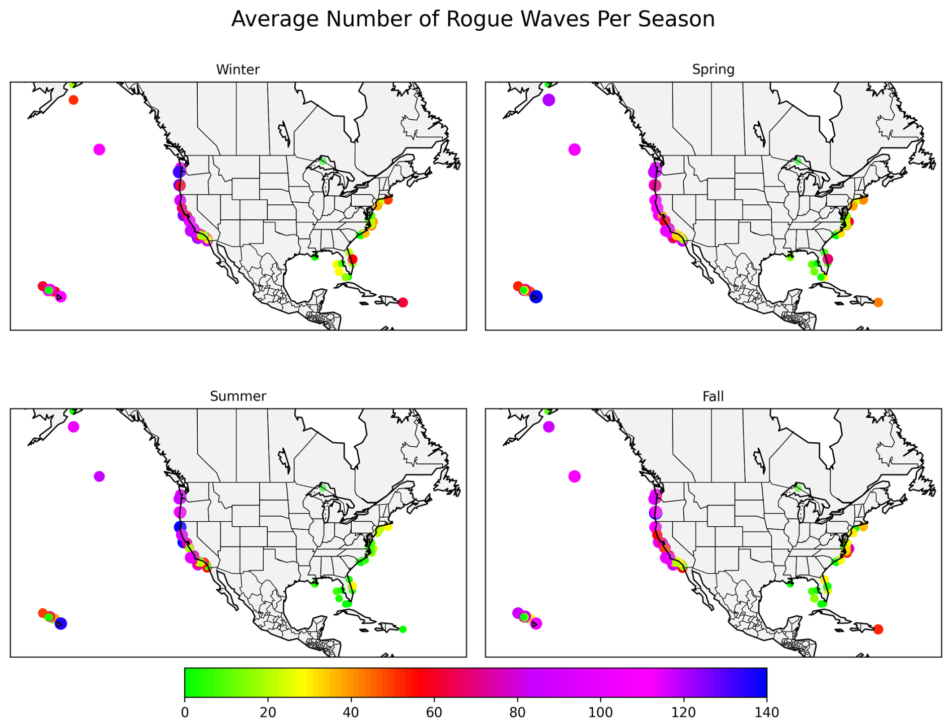
Figure 1 Average number of rogue waves per season based on CDIP buoy data from the FOWD dataset from 2015 to 2021. Color gradients represent the average number of rogue waves detected per season at each buoy location. Seasons are defined as: Winter from December to February, Spring from March to May, Summer from June to August and Fall from September to November.

The seasonal distribution of rogue waves seems to follow a trend influenced by large-scale meteorological and oceanographic processes (Wang and Swail, 2001). Counts range from tens to over one hundred per season regionally, with a winter maximum on the U.S. West Coast and a summer minimum basin-wide. Rogue waves are most frequent in the Winter season, with the West Coast experiencing peak values of 100 to 150 events per season in certain locations (Cattrell et al., 2019). The Northeast U.S. and Mid-Atlantic also show increased occurrences, with 50 to 100 events per season at some buoys. This is consistent with the dominance of extratropical storm activity in the North Pacific and North Atlantic, which generates high-energy wave fields conducive to nonlinear wave interactions that form rogue waves. A moderate decline in rogue wave occurrences is observed in the spring. Along the West Coast, values drop to 60–100 events per season, while the East Coast sees a reduction to around 40–70 events per season. This seasonal shift is likely related to the weakening of winter storms and the transition into calmer springtime wave conditions. During summer, rogue wave occurrence along the U.S. West Coast remains elevated in the northern sectors (Oregon and Washington), with many buoy locations recording approximately 60–120 events per season, while central and southern California exhibit substantially lower values, typically below 40–60 events per season. This pronounced north–south gradient contrasts with winter, when high rogue wave counts (60–140 events per season) extend more uniformly along much of the West Coast. This spatial pattern reflects the persistence of energetic swell and storm-generated wave fields in the Pacific Northwest during summer, whereas southern California experiences more sheltered and swell-filtered conditions. The Hawaiian region still exhibits moderate occurrences, around 30–60 events per season, possibly due to long-period swells generated by distant storms. And in the fall, there is a resurgence in rogue wave occurrences, particularly along the West Coast, where values climb back to 80–120 events per season. The East Coast also sees an increase, with values reaching 40–80 events per season. This seasonal uptick aligns with the intensification of storm activity as the transition to winter begins.

The strong winter peak in rogue wave occurrences, especially along the West Coast and North Atlantic, corresponds to the seasonal intensification of extratropical cyclones, which generate unstable sea conditions, large wave fields and steep wave conditions favorable for rogue wave formation. We attribute winter dominance to high-energy, steep, multi-modal seas and group dynamics, without asserting a specific nonlinear mechanism. The summer minimum is expected, as storm activity diminishes, leading to a calmer sea state in general. The fall and spring transitional periods show moderate rogue wave activity, reflecting seasonal shifts in storm intensity and frequency. In this study “unstable sea conditions” denotes high steepness, rapidly evolving or multi-modal spectra, and shifting directionality under strong synoptic forcing.

Whisker plots were created (Fig. 2) to present the monthly distribution of significant wave height (H_s) and maximum individual wave height (H_max) our three distinct data sources: CDIP-FOWD (buoy observations), ERA5 (reanalysis), and ECMWF CY47R1 (high-resolution hindcast). Whiskers quantify distribution spread; we assess rogue occurrence where $H_{\max }/H_{\mathrm{s}}$ and explicit event counts are analyzed. FOWD buoy records use 30 min time windows; model fields are hourly. We collocate by nearest grid point and compare each hourly model output to the closest-center buoy record. Event composites use 72 h windows (±36 h) around the rogue timestamp. The ERA5 and the ECMWF datasets have been filtered to match exactly the FOWD dataset, meaning there was no data considered when spectral significant wave height $H_{m_{\mathrm{0}}}<\mathrm{1}$ m. This provided not only insights into the seasonal variations, but also aimed to show the discrepancies between datasets, and implications for rogue wave identification. The central box represents the interquartile range (IQR), which contains the middle 50 % of the data points (from the 25th to the 75th percentile). The horizontal line inside the box represents the median value of the dataset for each month. The whiskers extend to 1.5 times the IQR or the minimum and maximum non-outlier values. The small hollow black circles represent outliers, which are values that exceed the whisker range and indicate extreme wave events.

The presence of numerous outliers, particularly in H_max, suggests that extreme wave occurrences are common, especially in winter months. These outliers are particularly relevant because rogue waves are extreme events, and their detection relies on capturing these deviations from the general wave height distribution. The smaller number of extreme outliers (isolated black circles) in ERA5 and ECMWF CY47R1 suggests they do not fully capture rogue waves, supporting previous studies that indicate reanalysis datasets smooth out extremes.

Figure 2 Whisker plots representing statistics of maximum wave heights (in meters) and significant wave height (in meters) per month for the buoy data (all locations combined from the FOWD dataset), the ERA5 dataset and the ECMWF dataset for the same period, from 2015 to 2021. All datasets have been filtered so there is no data when $H_{m_{\mathrm{0}}}<\mathrm{1}$ m. Buoy H_max from zero-crossings; model 〈H_max〉 is envelope-based.

The highest values of H_max and H_s occur in January, February, and December, with numerous H_max outliers exceeding 20–25 m and extreme values surpassing 30 m, and several H_s outliers exceeding 10 m. The median H_max during winter months is about 4 m across the datasets (with long tails), while H_s values are typically between 2.5 and 3.5 m. These months also exhibit the widest interquartile ranges and the greatest number of high-end outliers, reflecting more energetic and variable sea states associated with winter storm systems. Summer months show a notable decrease in wave energy, with H_max medians between 3.5 and 4.5 m and H_s between 1.5 and 2.5 m across all sources. During summer, fewer outliers are present and the whisker spread is narrower, indicating calmer and more stable sea states. In transitional seasons such as fall and spring, from September to November and April to May, there is a gradual broadening in the spread of both H_max and H_s values, illustrating a progressive return to more dynamic and energetic conditions.

Comparing H_max across the datasets, all three – FOWD (yellow), ERA5 (blue), and ECMWF CY47R1 (red) – show similar medians, with FOWD generally capturing more high-end outliers, indicating a potential underestimation of extreme wave events from models. ERA5 and ECMWF show strong agreement in median H_max values throughout the year, although ERA5 occasionally reports slightly lower medians. The FOWD dataset however presents a lower value throughout the distribution, on the box values and medians, which may reflect limitations in mooring response causing underestimation of the highest wave crests in some conditions. The reason why the model and reanalysis systematically show higher H_max values is likely due to the different methods how to calculate H_max. The maximum height based on individual waves is lower than the maximum envelope height (see Fig. 1 in Cicon et al., 2024). In addition, buoys often record lower wave heights because they can be pushed underwater by the crest or drift sideways, missing the very top of the wave (Forristall, 2000). Another reason is that buoys tend to move forward with the wave when they're on the crest and backward in the trough, which means they spend more time on the crests. This movement slightly raises the average sea level they record, but at the same time causes them to underestimate how tall the highest wave crests really are (Forristall, 2000).

It must be noted that the models compute H_max from the statistical properties of the wave envelope rather than by tracking each wave crest directly. Both ERA5 and ECMWF calculate H_max as an expectation from the envelope-based statistical distribution of wave heights 〈H_max〉, adjusted for number of waves and spectral shape (Janssen, 2003, 2005, 2015). Though this yields reasonable agreement with aggregate buoy statistics, it is inherently limited in capturing individual extreme crests – especially rogue waves – because it smooths over actual variability and rests on Gaussian assumptions. Consequently, peak wave events can be underrepresented relative to in situ measurements. In addition, overestimation may occur because 〈H_max〉 is a mean of the extreme-value distribution rather than a single observed crest.

For H_s, the agreement across all datasets is more consistent. Median and interquartile values for H_s are nearly identical during most months, particularly in summer, suggesting strong convergence of model and observational estimates once the data have been consistently filtered to exclude low-energy sea states. FOWD displays slightly lower H_s values, especially in summer months, but otherwise aligns closely with ERA5 and ECMWF. All three datasets reproduce the expected seasonal modulation of significant wave height with strong fidelity.

The monthly whisker plots infer that extreme wave occurrences are more frequent when overall wave energy is higher. The direct correlation between high H_s and extreme H_max values supports the conclusion that the probability of extreme waves increases during high-energy sea states. Winter and fall periods show the highest wave heights, aligning with the most frequent rogue wave occurrences in the seasonality map. Summer shows the lowest wave heights, with minimal rogue wave occurrences, consistent across both graphs. Spring acts as a transitional phase, with moderate values in both wave height and rogue wave frequency. The west coast domination in rogue wave events suggests that high wave height alone is not the only factor for rogue wave formation; local bathymetry, wave-current interactions, and linear and nonlinear effects also likely play a role (Cattrell et al., 2018).

Scatter density plots are also a powerful tool for visualizing the relationship between two different datasets (Fig. 3) (Cicon et al., 2024). Each point in the scatter plots below represents a pair of values, with FOWD buoy measurements on the x-axis and the corresponding values from ERA5 or ECMWF CY47R1 on the y-axis. The correlation coefficient (r-value) in each plot quantifies how well the model data aligns with the buoy measurements, with values closer to 1.0 indicating a stronger agreement.

Analyzing the Maximum Individual Wave Height (H_max) graphs, the ERA5 vs. FOWD plot in the upper left panel shows a Pearson correlation coefficient of r=0.90, indicating a strong agreement between model and observational data in estimating H_max. Most of the data points cluster along the 1:1 line, particularly for wave heights between 2 and 10 m, suggesting that ERA5 captures the general behavior of sea states within this range. Beyond 10 m, however, a tendency for underestimation becomes more apparent, with ERA5 values falling below the FOWD observations. In the upper right panel, ECMWF also achieves a Pearson correlation of r=0.90 with FOWD for H_max, and displays a similar distribution to ERA5, including the same systematic underrepresentation of extreme wave heights greater than 12 m. The red regression lines lying slightly below the 1:1 line at high H_max values, confirm that the models underestimate peak extremes.

For the Significant Wave Height (H_s) scatter plots, both ERA5 and ECMWF show slightly stronger correlation with FOWD, with r=0.92 in both cases, highlighting better model fidelity in representing bulk sea state energy. These panels show an even tighter clustering along the 1:1 line, suggesting excellent agreement in H_s values across the range of 1.5 to 6 m. A few deviations can be observed above 7 m, where the models show a slight negative bias. The high density around H_s values of 2.5 to 4 m reflects the prevalence of energetic but not extreme wave conditions. Overall, both ERA5 and ECMWF reproduce H_s behavior well in storm and swell-dominated regimes, capturing the bulk statistical structure of significant wave height with minimal error. These scatter plots use the FOWD H_s time-domain parameter rather than spectral $H_{m_{\mathrm{0}}}$, allowing lower-bound values to be included near the 1 m filter threshold.

Figure 3 Density Scatter Plots of ERA5 reanalysis vs. FOWD buoy data and ECMWF CY47R1 hindcast vs. FOWD buoy data for maximum wave height (H_max), significant wave height (H_s) and rogue wave index ($H_{\max }/H_{\mathrm{s}}$) for all buoy locations for the years of 2015 to 2021 (inclusive). The color gradient represents the density of points, where warmer colors (red/yellow) indicate a higher concentration of data points and cooler colors (blue) represent lower densities. All datasets are filtered so there is no data when $H_{m_{\mathrm{0}}}<\mathrm{1}$ m. Buoy H_max from zero-crossings; model 〈H_max〉 is envelope-based.

In contrast, the bottom row of the figure, representing the $H_{\max }/H_{\mathrm{s}}$ ratio (the rogue wave index) reveals a near-total lack of correlation between the models and the FOWD dataset. For ERA5, $H_{\max }/H_{\mathrm{s}}$ values are tightly clustered between 1.6 and 2.0, suggesting that the model suppresses variability in this ratio and rarely reflects the presence of rogue waves. FOWD data, on the other hand, span a wider range from approximately 0.2 to 3.2, capturing extreme wave amplification events more effectively. ECMWF shows slightly improved variability, with values concentrated between 1.7 and 2.2, and more frequent occurrences of $H_{\max }/H_{\mathrm{s}}$ > 2.0 than ERA5. However, both models exhibit evident bias and range compression, confirming their limited capacity to resolve extreme and rogue wave events. This bias on the $H_{\max }/H_{\mathrm{s}}$ model values may occur due to the nature of the models' H_max calculation, which is intrinsically connected to H_s.

While both ERA5 and ECMWF exhibit strong correlations for independent parameters like H_max and H_s, their inability to represent the ratio $H_{\max }/H_{\mathrm{s}}$ reflects their failure to account for transient, localized wave amplification phenomena. This finding corroborates earlier studies suggesting that coarse model resolutions and temporal averaging suppress extreme features such as rogue waves (Campos et al., 2018; Lobeto et al., 2024; Hersbach et al., 2020). Both ERA5 and ECMWF aggregate wave statistics over spatial grid cells of approximately 40 and 18 km, respectively, which inherently dampens localized peaks observed by high-frequency buoy measurements.

Probability density function (PDF) graphs were additionally created to represent the likelihood of different values occurring within a dataset (Fig. 4) (Nederkoorn and Seyffert, 2022).

Although all three datasets exhibit a similar shape of PDF distributions for Maximum Individual Wave Height (H_max), the FOWD dataset reveals a slightly broader spread and a longer tail toward extreme values. FOWD shows a higher standard deviation (1.69 m) and a maximum H_max of 30.49 m, compared to 19.75 m in ERA5 and 19.71 m in ECMWF. This difference illustrates that FOWD buoys capture extreme wave events more frequently, possibly due to their high temporal resolution and ability to resolve short-lived energy peaks in real time. In contrast, the spectral models tend to smooth out such extremes, leading to a truncation of the right tail in the model distributions.

The same trend is reflected in the Significant Wave Height (H_s) PDF, where FOWD shows slightly elevated variability, with a standard deviation of 0.935 m and a maximum H_s of 12.22 m. While ERA5 and ECMWF follow similar central tendencies, both exhibit slightly narrower distributions and reduced peak values (ERA5 H_s max = 10.39 m; ECMWF H_s max = 10.23 m). The broader distributions and higher extremes in FOWD are consistent with a heavy-tailed probability structure – potentially resembling a Fréchet-type distribution – characteristic of rogue wave–prone sea states. The slow decay of probability towards very high (extreme) values, which is common for ocean extremes and suggests that events significantly greater than the mean occur more frequently than would be predicted by normal or exponential distributions.

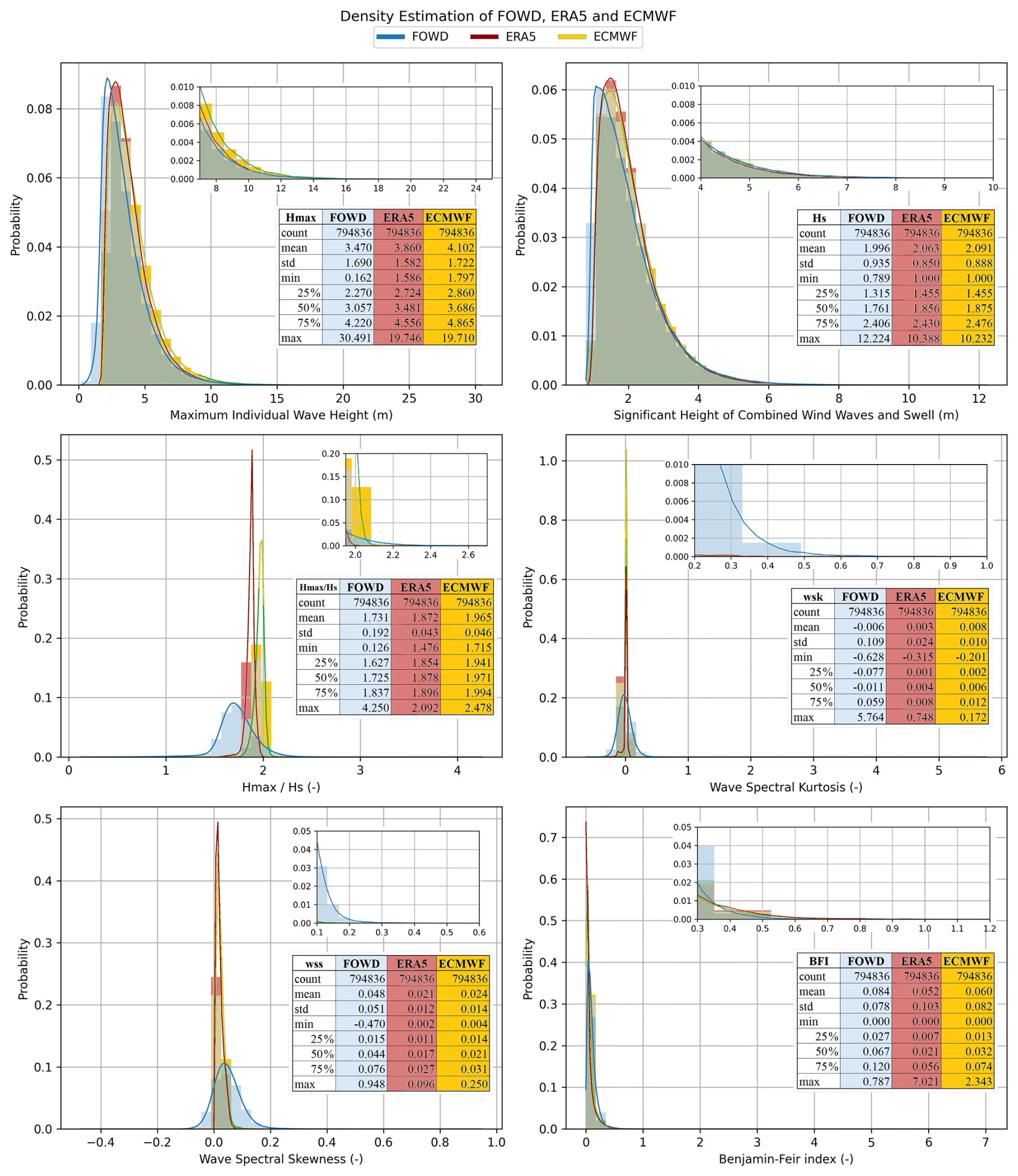
Figure 4 Probability Density Functions of different wave parameters comparing data from buoys (FOWD dataset), depicted in blue, the ERA5 reanalysis depicted in red and the ECMWF CY47R1 hindcast depicted in yellow for the same period, from 2015 to 2021. The zoom of the positive tail is depicted at the upper right. Basic Statistics are shown on the tables. All three datasets are filtered so there is no data when $H_{m_{\mathrm{0}}}<\mathrm{1}$ m. Buoy H_max from zero-crossings; model 〈H_max〉 is envelope-based.

In the rogue wave index ($H_{\max }/H_{\mathrm{s}}$) PDF, the FOWD dataset shows a broader distribution with a strong peak between 1.6–1.8, which depicts the relationship we usually see in real life, with a wider range of wave amplification scenarios, where extreme waves are less common (Nederkoorn and Seyffert, 2022). FOWD also shows a much longer tail with a broader distribution and with more points exceeding 2, meaning it captures more rogue wave events than ERA5 and ECMWF. In contrast, ERA5 and ECMWF data cluster more narrowly. ERA5 centers around 1.87 with a standard deviation of 0.043, while ECMWF clusters slightly higher, around 1.97 with a standard deviation of 0.046. This artificial narrowing suggests a systematic model bias which is not always seen in real life (Janssen, 2015). While ECMWF slightly improves upon ERA5 in mean values, neither captures the full spread of the observational data.

Wave spectral skewness (3rd standardized moment of surface elevation) measures the asymmetry of the wave spectrum, characterizing how energy is distributed across wave frequencies (Stansell, 2004). High skewness values are often linked to wave focusing mechanisms, which amplify extreme events. Previous research (Mori and Janssen, 2006) attests that skewness is a good predictor of rogue wave formation, particularly in shallow water. The FOWD data show a broader and more variable distribution of skewness values (ranging from −0.47 to 0.95), with a mean of 0.048 and a notably higher standard deviation compared to both ERA5 and ECMWF. In contrast, the models are tightly centered near zero with very low variability, reflecting an inability to represent asymmetrical and steep wave structures. This has implications for rogue wave detection, as wave asymmetry has been shown to precede extreme crest formation.

Wave spectral excess kurtosis (4th moment of surface elevation minus three), which reflects the “peakedness” or spectral concentration of wave energy (Goda, 1970), where higher kurtosis values have been linked to increased rogue wave probabilities, as they indicate wave focusing mechanisms (Mori and Janssen, 2006; Mori et al., 2011). Theoretical work (Fedele et al., 2016) suggests that spectral peakedness (high kurtosis) is a necessary condition for rogue waves to form. The FOWD dataset records kurtosis values extending above 5.7 with a standard deviation of 0.109, while ERA5 and ECMWF are constrained to low values near 0, suggesting Gaussian-like behavior.

FOWD data demonstrates both more positive skewness and elevated kurtosis values, indicating frequent departures from Gaussian behavior in the wave field. These are signatures of asymmetric, steep, and strongly peaked wave groups, conditions known to precede rogue wave events. In contrast, both ERA5 and ECMWF exhibit distributions that are centered near zero with low variability, highlighting their lack of sensitivity to wave shape irregularities and spectral sharpness.

The Benjamin-Feir Index (BFI) is a dimensionless parameter associated with modulational instability. High BFI values (> 1) are typically associated with increased likelihood of rogue wave generation in deep water (Onorato et al., 2005; Janssen, 2003). In the BFI PDF, the FOWD dataset again exhibits a broader distribution with a mean of 0.084 and broader overall distribution, indicating its sensitivity to modulational instability. ERA5 and ECMWF present minimal spread, again indicating their lack of ability to resolve the nonlinear physics critical for rogue wave development (Janssen, 2015). Both ECMWF and ERA5 present very high outliers as maximum values, this appears as a rare artifact and does not reflect reality.

Collectively, these findings confirm that buoy measurements provide a more robust representation of real-world wave variability, including the physical and spectral conditions conducive to rogue wave formation. The inability of ERA5 and ECMWF to replicate the variability in all parameters indicates fundamental limitations in their spatial resolution, data assimilation strategies, and reliance on linear spectral parameterizations. These constraints lead to the systematic underestimation of extreme wave phenomena and reduce the utility of model-based datasets for rogue wave forecasting.

3.2 Specific Rogue Wave Events Analysis

Recent advances in ocean wave dynamics, particularly the work of Dion Häfner et al. (2021a, b), emphasize the importance of additional spectral parameters in improving rogue wave prediction and classification (Hafner et al., 2021b). These include spectral bandwidth narrowness, the relative energy contained within the 0.25–1.5 Hz range, and crest-trough correlation. By incorporating these parameters into the analysis, it is possible to gain a more refined understanding of wave evolution and the mechanisms leading to rogue wave amplification.

In this study, we looked at four rogue wave occurrences in four different CDIP buoy stations to more deeply investigate the sea state evolution before, during and after a rogue wave event. The buoys' FOWD data parameters of interest were mainly compared to the ECMWF CY47R1 wave hindcast data from 2015 to 2021, which also included the global values for crest-trough correlation, relative energy on the 0.25 to 1.5 Hz frequency and the narrowness spectral bandwidth based on Hafner's formulas. For the more usual parameters maximum wave height, significant wave height and the rogue wave index, which is just one divided by the other (H_max divided by H_s), we also compared with the ERA5 reanalysis data and the non-filtered CDIP data, directly from calculations from the heave (surface elevation) raw data from the CDIP archives. The selected buoys – Mokapu Point, HI (098), Block Island, RI (154), Clatsop Spit, OR (162), and Ocean Station Papa (166) – are positioned in distinct oceanic regions, providing datasets for understanding the conditions that contribute to rogue wave events in different environments (Fig. 5).

The North Pacific, represented by Ocean Station Papa (166), is characterized by persistent long-period swells and high-energy wave climates, a good location for studying nonlinear wave interactions. Block Island (154) can be influenced by extratropical storm activity, providing an opportunity to examine how synoptic-scale weather systems impact rogue wave generation. Clatsop Spit (162), positioned along the Pacific Northwest, is subject to both local wind-driven waves and open ocean swells, offering a complex wave climate for spectral analysis. The Mokapu Point buoy (098) in Hawaii captures wave data in a region where energy is frequently influenced by trans-Pacific swell propagation and episodic storm activity.

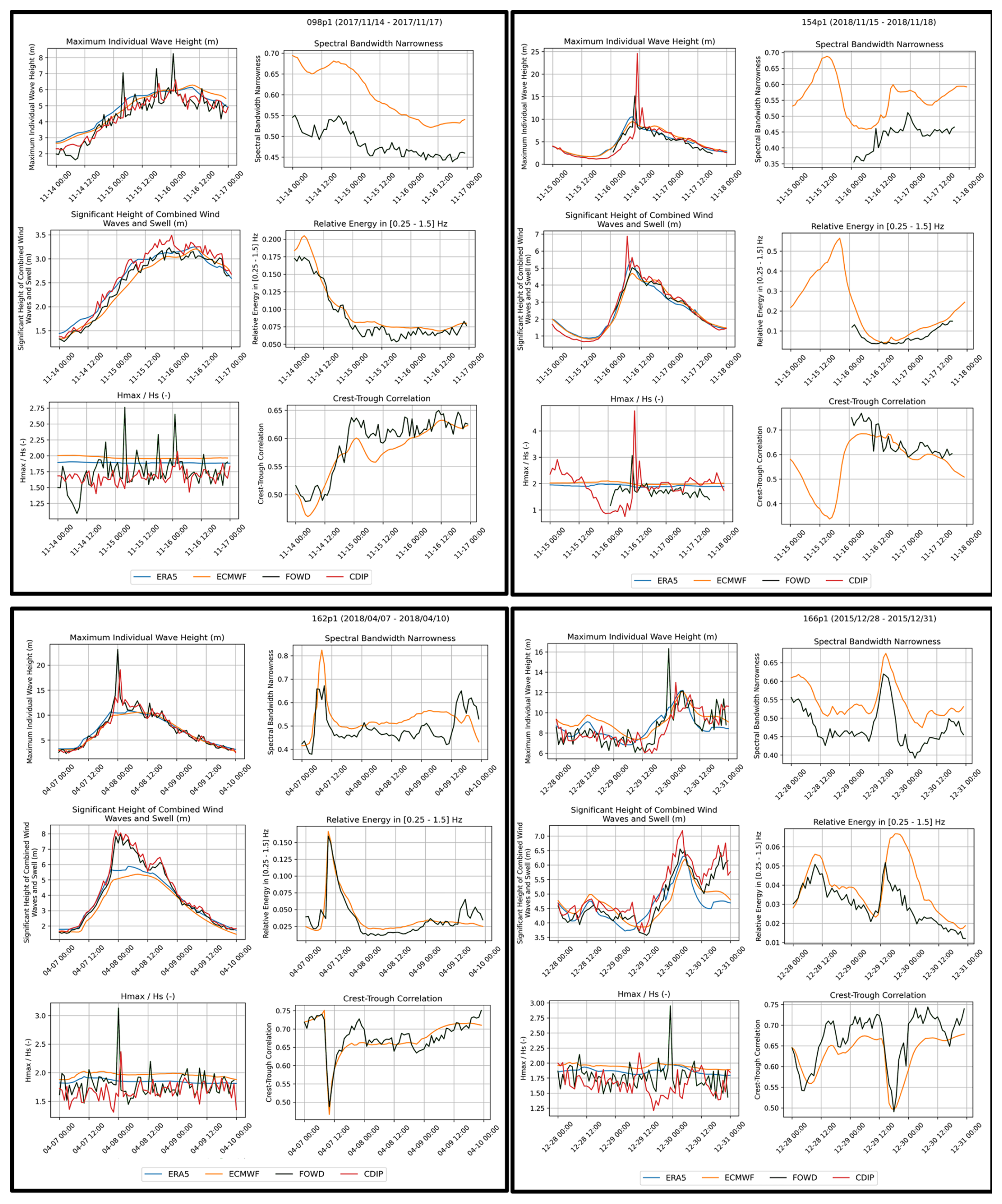
Figure 5 Specific rogue wave event analysis at four different buoy stations (098, 154, 162, and 166) during a period of 72 h. ERA5 data is depicted in blue, ECMWF CY47R1 data depicted in orange, FOWD data depicted in in black and raw CDIP data depicted in red. Buoy H_max from zero-crossings; model 〈H_max〉 is envelope-based.

We re-audited IDs, timestamps, units, and quality control (QC). Residual differences occur where FOWD QC excludes short segments around spikes. We flag such windows in Fig. 5 and harmonize the 72 h windowing. We first note that in the four locations graphs the calculations based on the raw, non-filtered, CDIP surface elevation data (in red) usually does not match 100 % with the filtered CDIP data calculation from the FOWD dataset (in black). When using the raw, non-filtered, data, we sometimes see rogue waves peaks (when data goes above 2 on the $H_{\max }/H_{\mathrm{s}}$ graphs) that were not present on the filtered data. For future studies, it is important to check if perhaps the filter CDIP and others are using are not unintentionally removing real rogue waves events, which could be perceived as non-real outliers, from the data. The usual modelled data (ERA5 or ECMWF) smoothing can also be clearly noticed in all the graphs from Fig. 5.

Observational data from the selected rogue wave events at stations 098, 154, 162, and 166 consistently demonstrated that a decrease in crest-trough correlation was accompanied by a simultaneous narrowing of spectral bandwidth and an increase in relative energy within 0.25–1.5 Hz. This suggests that these spectral changes occur in tandem with the restructuring of the wave field, marking a transition phase where rogue waves are more likely to emerge. The spectral focusing effect, driven by spectral narrowing with elevated relative energy in 0.25–1.5 Hz, leads to an increase in wave amplitude variability and supports the formation of extreme, isolated waves.

4 Discussion

The crest-trough correlation parameter is strongly linked to spectral bandwidth, with narrower bandwidths leading to more correlated wave structures (Cicon et al., 2024). This relationship is crucial because wave groups in bandwidth-limited conditions favor rogue wave development. Studies using buoy observations from the FOWD dataset and wave modeling with WAVEWATCH III (WW3) show that high crest-trough correlation values (> 0.6) are associated with rogue wave probabilities that are an order of magnitude higher than in uncorrelated wave fields (Cicon et al., 2023). Häfner et al. (2021b) showed that rogue wave probability of occurrence varies by a factor of 10 based on crest-trough correlation alone, far exceeding the indicator capability of parameters like kurtosis, skewness, or steepness. And unlike kurtosis, which is only useful within single wave groups, crest-trough correlation remains a reliable predictor across extended time periods and different oceanic regions. Since crest-trough correlation can be calculated from wave spectra moments, it can be directly implemented into operational wave forecast models like those run by ECMWF and NOAA.

The link between spectral bandwidth narrowness, relative energy and the crest-trough correlation parameter can be understood through their combined impact on wave evolution. As spectral bandwidth narrows, wave energy is confined to fewer dominant modes, reducing spectral dispersion and increasing the likelihood of constructive interference. This effect is further amplified when energy in the 0.25–1.5 Hz range increases, signifying a shift toward wave fields where co-existing swell adds a quasi-stationary low-frequency partition; and the transient group beating between partitions modulates short-term envelope statistics. Swell components reinforce the background wave spectrum rather than dissipating across a broader range of frequencies. This process results in enhanced wave group formation, where wave trains become more phase-aligned over time, increasing the crest-trough correlation values and consequently the probability of extreme wave occurrences.

Häfner's FOWD introduction article (Hafner et al., 2021a) contains a probability density function (PDF) graph for crest-trough correlation parameter r for all FOWD waves. It shows a distinction in correlation values between all waves, waves with $H_{\max }/H_{\mathrm{s}}>\mathrm{2}$ (moderate rogue waves), and waves with $H_{\max }/H_{\mathrm{s}}$ > 2.4 (extreme rogue waves). For all waves, the crest-trough correlation (r) values are broadly, almost normally, distributed across a range spanning approximately 0.2 to 0.9, with a peak around 0.6 to 0.7. For waves that have a height that is more than twice the significant wave heigh, the crest-trough correlation distribution shifts a bit toward higher values, with most cases occurring above 0.5, and the peak moving toward 0.7 to 0.8. And for extreme rogue waves (rogue wave index > 2.4), the crest-trough correlation range is even more constrained, with most values falling between 0.6 and 0.9, and a pronounced peak around 0.75 to 0.85. This strong shift toward higher correlation values confirms that rogue waves tend to form in conditions where wave crests and troughs are highly correlated, reinforcing the role of linear superposition in rogue wave generation. On the other hand, this PDF clearly shows that it is not possible to consider a 0.6 or 0.7 crest-trough correlation parameter threshold alone to identify rogue waves since in general seas the values go up to 0.9 with most values around 0.6.

While it is well established that rogue waves are better sustained in sea states where the crest-trough correlation remains above 0.6 due to wave groupness and focusing, this alone does not serve as an effective predictor. Instead, it is the preceding conditions – a temporary drop in crest-trough correlation followed by a rapid increase – that provide a more reliable early warning indicator. This finding suggests that rogue waves tend to emerge in dynamically evolving sea states rather than in purely steady conditions. For a rogue wave warning system, the focus should not be solely on identifying when crest-trough correlation exceeds 0.6, but rather on recognizing the transition phase that precedes it. By monitoring the evolution of crest-trough correlation in combination with spectral bandwidth changes and relative energy shifts, it may be possible to establish a probabilistic framework for forecasting rogue wave risk.

Across all four locations on Fig. 5, the evolution of this parameter follows a distinct sequence where an initial decrease in crest-trough correlation below 0.5 is observed, followed by a rapid increase exceeding 0.6 just prior to or during the rogue wave event. This pattern strongly suggests that rogue wave conditions are preceded by a transitional phase in the wave field, where wave coherence temporarily weakens before re-emerging in a more clustered and structured state, favoring the onset of extreme wave amplification.

At Station 154 (Block Island, RI), a pronounced rogue wave event occurs on 16 November 2018, with a sudden spike in H_max exceeding 20 m. Prior to this event, crest-trough correlation drops below 0.5, followed by a rapid recovery above 0.6. Concurrently, spectral bandwidth narrowness increases, indicating that wave energy is being redistributed into fewer dominant frequencies, a process that aligns with constructive interference mechanisms. The rogue wave event is marked by an increased crest-trough correlation, reinforcing the idea that high correlation values ($>\sim$ 0.6) sustain rogue waves, but the transition from a lower correlation state is what signals their imminent formation.

A similar pattern was evident at Station 162 (Clatsop Spit, OR) during the rogue wave occurrence on 8 April 2018. The crest-trough correlation parameter initially dropped sharply, reaching a minimum near 0.45, before rising to values exceeding 0.65 just as the rogue wave event occurred. This sequence was accompanied by an increase in relative energy within the 0.25–1.5 Hz range, indicating a strengthening of the short-wave wind sea component. The simultaneous rise in crest-trough correlation and dominance of wind-sea energy suggests that the wave field became increasingly organized and energetically focused, creating favorable conditions for nonlinear wave amplification. This relationship between evolving spectral energy and coherence supports the notion that rogue waves emerge during transient dynamical transitions.

At Station 166 (Ocean Station Papa), the rogue wave event on 30 December 2015, follows the same pattern, with crest-trough correlation first dropping below 0.5, signaling a reduction in wave coherence, and then recovering above 0.6 immediately before the rogue wave appears. This behavior is accompanied by increasing spectral bandwidth narrowness and rising relative energy levels, reinforcing the finding that the restructuring of wave groups precedes rogue wave formation.

These observations confirm that while rogue waves are better sustained in seas where crest-trough correlation remains above 0.6, which means this is a robust rogue wave identifying condition, however this parameter alone is not a sufficient predictor. Instead, the transition phase, where crest-trough correlation temporarily decreases before increasing again, appears to be a more reliable precursor to rogue wave formation.

To statistically verify the accuracy of this inverted peak, or drop on the crest-trough correlation, hypothesis in relation to rogue wave identification, we performed an analysis using the data from the FOWD quality-controlled dataset. Data available for stations 154, 162, 166 and 098 between 2015 and 2021 were gathered, and the total number of rogue waves was found simply checking the relative height parameter being larger than 2. This parameter is the calculated H_max divided by the spectral significant wave height every 30 min. There were 81 rogue waves found. Note that the FOWD dataset is filtered to contain only waves with significant heights above 1 m, which translates to rogue waves with a 2 m height minimum. Then we downloaded the date related crest-trough correlation parameter from 1.5 d before and 1.5 d after the located rogue wave event. During this time, we looked for the inverted peak that had a minimum 0.1 difference in the crest-trough correlation values and that reached a correlation of 0.5 or below. We found 61 instances that agreed with our hypothesis, which means that 75 % of the rogue waves followed our criteria. This suggests that a real-time rogue wave warning system should focus on detecting this sharp drop and recovery in crest-trough correlation, rather than merely identifying when values exceed a threshold. Approximately 25 % of rogue events did not meet the inverted-r criterion. Typical scenarios include: (i) persistent swell with high r but no preceding dip; (ii) mixed/transitioning seas where r is noisy and dips are < 0.10; (iii) removal of short segments by QC near the event; or (iv) r_min slightly > 0.50 before rebound. We have not quantified false positives (inverted-r without a subsequent rogue) but we will do so in future, longer studies with more data.

Cicon et al. (2024) proposed an empirical formula which initially expressed rogue wave occurrence probability as a function of certain parameters, including wave steepness, relative depth, directional spread, and spectral bandwidth, alongside with the crest-trough correlation (r) parameter. However, after evaluating the performance of this formula using buoy observations and ECMWF hindcast data, they found that the inclusion of these additional variables offered only limited improvement in predictive skill, since the coarse resolution of global models usually fail to accurately capture nonlinear effects, particularly in shallow water environments, where these parameters are expected to play a more significant role. So, Cicon et al. (2024) computed a simplified version of the empirical formula in which steepness, relative depth, directional spread, and spectral bandwidth are replaced with their mean values, reducing the equation to a function of only r and two empirical constants (Cicon et al., 2024).

While Cicon et al. equation showed an improved fit to in-situ data only using the crest-trough correlation parameter, like our study, we do not numerically compare our results to hers because the studies targets and definitions differ. We propose that predictive power can be improved if, instead of considering only the absolute value of r at a given moment in time, the models also account for its temporal evolution. Our goal is to work on the implementation of this model for our future work.

5 Conclusions

This study provides an initial assessment of wave models and rogue wave occurrences by comparing in situ observations from FOWD (Free Ocean Wave Data) buoys with model-based estimates from ERA5 reanalysis and the ECMWF CY47R1 high-resolution hindcast. By integrating multiple analyses, including seasonal rogue wave distributions, statistical comparisons of maximum wave heights (H_max) and significant wave heights (H_s), and density scatter plots with additional spectral parameters (skewness, kurtosis, and BFI), we identified critical differences in how rogue waves are represented across these datasets. Furthermore, this research aims to validate the effectiveness of crest-trough correlation as a leading indicator of rogue wave risk while evaluating the role of spectral bandwidth and energy distribution in wave amplification processesin deep-water.

A map analysis of rogue wave occurrences from the FOWD dataset revealed a strong seasonal dependence, with peak rogue wave activity occurring in winter and fall and the highest concentrations of rogue waves found along the West Coast and then the North Atlantic. This corresponds to the seasonal intensification of extratropical cyclones in these areas. The Gulf of Mexico and the southeastern U.S. coastline exhibit significantly lower rogue wave occurrences, likely due to a calmer wave climate.

The monthly whisker plots of H_max and H_s strongly supports these seasonal findings. Maximum wave heights and significant wave heights peak in winter, with median H_s values of combined wind waves and swells reaching 2–3 m and extreme H_max values exceeding 20 m. The presence of numerous outliers in winter months suggests a greater probability of rogue wave formation during storm-driven high-energy sea states. Summer, on the other hand, shows the lowest wave activity, with median H_s values of 1.5–1.8 m and H_max median values between 2.5–4 m and the extremes reaching 13 m maximum, corresponding to a minimum in rogue wave occurrences. Further studies pursuing the analysis of the regionalization of this data are recommended.

The model data from ERA5 reanalysis and ECMWF CY47R1 hindcast systematically underestimated extreme wave events, particularly for higher maximum individual wave heights (H_max). While both models exhibit strong correlations with FOWD measurements (r≈0.90–0.92 for H_max and H_s), their distributions show a consistent bias toward lower values. The density scatter plots confirm that ERA5 and ECMWF align well with FOWD for moderate sea states (H_max<10 m) but significantly underestimate extreme values (> 15 m). This suggests that model smoothing and spatial averaging limit their ability to resolve transient, high-energy wave events, which are critical for rogue wave detection. Phase-averaged global models reproduce bulk statistics (H_s, moderate H_max) but under-represent the tails ($H_{\max }/H_{\mathrm{s}}$), consistent with envelope expectations and grid-scale averaging.

The buoys FOWD data frequently records a lot more rogue wave occurrences if compared to ERA5 and ECMWF model data. The scatter plots of $H_{\max }/H_{\mathrm{s}}$ reveal that both models cluster tightly around values near 2.0, whereas FOWD displays a broader distribution with a higher incidence of $H_{\max }/H_{\mathrm{s}}>\mathrm{2.5}$, demonstrating that rogue waves are significantly underrepresented in reanalysis and hindcast datasets. This underestimation may be linked to the method the models use to calculate H_max, to the smoothing of extreme values and limited representation of nonlinear wave interactions in model parameterizations (Campos et al., 2018; Lobeto et al., 2024).

A few spectral parameters recognized to influence rogue wave formation were also analyzed on probability density functions: wave spectral skewness, spectral kurtosis, and the Benjamin-Feir Index (BFI). The buoys FOWD data exhibited a broader skewness, kurtosis and BFI distribution, capturing more variability in wave shapes compared to ERA5 and ECMWF, which cluster tightly around zero, indicating a lack of asymmetry, peakedness and instability in modeled wave spectra. These findings align with previous studies that suggest spectral wave models often rely on linear approximations, limiting their ability to resolve extreme wave dynamics (Janssen, 2015).

The underestimation of H_max, rogue wave occurrences, and nonlinear wave properties in ERA5 and ECMWF suggests that reliance on reanalysis and hindcast data alone may lead to underpredictions of extreme wave hazards. This is particularly concerning for the shipping industry, offshore energy platforms, and coastal infrastructure, where rogue waves pose serious risks (Bitner-Gregersen et al., 2015). The strong seasonal patterns identified in the FOWD dataset emphasize the need for seasonally adjusted forecasting models, particularly for high-risk regions such as the West Coast of the U.S. and the North Atlantic.

Lastly, specific rogue wave occurrences across four distinct locations were analyzed – Station 098 (Mokapu Point, HI), Station 154 (Block Island, RI), Station 162 (Clatsop Spit, OR), and Station 166 (Ocean Station Papa) from CDIP buoys. Across all stations, rogue waves were consistently preceded by a sharp drop in crest-trough correlation below 0.5, followed by a rapid recovery exceeding 0.6, indicating a transition from a less organized wave field to a more clustered and structured state. This pattern was accompanied by an increase in spectral bandwidth narrowness and relative energy in the 0.25–1.5 Hz range, suggesting that energy redistribution and constructive interference mechanisms play a significant role in rogue wave formation (Hafner et al., 2021b; Gemmrich and Thomson, 2017; Gemmrich and Cicon, 2022).

A statistical evaluation of this novel crest-trough correlation inverted peak hypothesis to identify rogue waves using FOWD buoy data showed a 75 % agreement. These findings reinforce previous studies that have highlighted crest-trough correlation as a dominant indicator of rogue wave probability, yet they also extend this understanding by demonstrating that the absolute value of the crest-trough correlation parameter should not be used as warning sign, but rather its dynamic evolution over time. While rogue waves are more likely to be sustained in environments where crest-trough correlation remains above 0.6, it is the transition from low to high correlation that signals their imminent formation. This provides a new perspective on how rogue wave forecasting could be approached, moving beyond static threshold-based indicators to a more dynamic assessment of wave evolution.

This study also highlights the need for more studies and forecasts to incorporate crest-trough correlation, narrowness spectral bandwidth and relative energy distributions as key parameters in rogue wave forecasting models. By integrating these parameters into the analysis, it is possible to refine forecasting methodologies and improve the understanding of rogue wave behavior across multiple oceanic environments. Additionally, by mapping these variables on a global scale using high-resolution wave models, it may be possible to identify regions where wave conditions are primed for rogue wave formation. These results from this study contribute to enhanced maritime safety, optimized offshore operational planning, and improved predictive models for extreme wave events.

Future studies should explore the operational integration of the crest-trough correlation parameter (r) to high-resolution wave models such as WAVEWATCH III and ECMWF operational forecasts. This would help identify rogue wave-prone areas based on spectral signatures and crest-trough correlation trends. Additionally, machine learning techniques can enhance predictive capabilities by assimilating large-scale model outputs with observed rogue wave occurrences, enabling the development of a probabilistic rogue wave forecasting system.