Turbulence and mixing along a microtidal and stratified estuary-shelf transition

This study investigates the hydrodynamic and mixing processes at the estuary–shelf transition of a microtidal system, and the buoyant plume generated at the Patos Lagoon mouth (Brazil). Using measurements of current velocities, salinity, temperature, and turbulent kinetic energy (TKE) dissipation (ϵ) during a high-discharge period (∼ 9400 m³ s⁻¹), we characterize the spatial evolution of turbulence and mixing along the channel, from the source to the buoyancy-driven plume region. Diagnosed using the internal Froude number, the observations showed a transition from sub-critical flow in the channel to super-critical flow in the buoyant plume liftoff zone, and back to sub-critical flow offshore. Despite strong stratification, intense shear-driven turbulence was observed, with TKE dissipation rates reaching 10⁻³ W kg⁻¹ near the mouth, comparable to values reported in high-energy mesotidal and macrotidal systems. Analysis of the buoyancy Reynolds number (Re_b) and the gradient Richardson number (Ri) indicates that inertial forcing overcomes buoyancy suppression, maintaining a predominantly turbulent regime (Re_b > 200) at the plume front. These results demonstrate that, in narrow, high-discharge estuarine outlets, the spatial evolution of turbulence and mixing reflects the combined influence of channel morphology, secondary circulation, and plume adjustment processes operating within a sustained supercritical flow regime, maintaining vigorous mixing even under pronounced density stratification.

1 Introduction

Buoyant plumes are critical hydrodynamic structures in coastal environments, as they represent the primary interaction in the flow transition between laterally constrained estuaries and the adjacent shelf (Fennel and Mutzke, 1997). Plumes are responsible for the injection of freshwater and momentum into the inner shelf, transporting suspended sediments, organic matter, nutrients, and pollutants (Horner-Devine et al., 2015). These inputs play a key role in regulating the coastal carbon budget by stimulating biological production and respiration on the inner shelf (Schettini et al., 1998; Cai et al., 2013; Lohrenz et al., 2013), thereby highlighting the importance of physical mixing in modulating these processes (Sims et al., 2022; Wu et al., 2023).

The dynamics of plumes are driven primarily by the density gradient between the low-salinity freshwater discharge and the denser coastal waters, as well as the momentum associated with the estuarine outflow (Horner-Devine et al., 2015; McPherson et al., 2019). These mechanisms control the plume's basic structure, including its lateral spreading, vertical layering, and the efficiency of mixing with the surrounding ocean. From a structural perspective, plume evolution has been described through a sequence of spatially distinct regions reflecting changes in the dominant physical processes (Jirka et al., 1981; Horner-Devine et al., 2015). These include: (i) a source region, strongly influenced by estuarine conditions and mouth geometry; (ii) a near-field region, characterized by jet-like behavior, beginning at the lift-off zone and dominated by inertial forces; (iii) a midfield region, where the influence of the initial discharge progressively weakens and the flow transitions from supercritical to subcritical conditions as the internal Froude number decreases below unity (Hetland, 2005); and (iv) a far-field region, associated with larger spatial scales, alongshore transport, and quasi-geostrophic dynamics.

Mixing plays a central role in the plume's spatial and temporal evolution, eroding vertical gradients and dissipating kinetic energy. This mixing occurs primarily through instabilities at the fluid interface, as well as through frontal processes and wind forcing (Ivey et al., 2008; Stacey et al., 2012; Spicer, 2022). However, direct turbulence measurements within the plume itself are notoriously difficult to perform, despite being fundamental for identifying and understanding the physical mechanisms responsible for mixing (Geyer et al., 2010). Although river plumes have been extensively studied, direct observations have generally been conducted at relatively sparse spatial and/or temporal scales. Consequently, a detailed description of transport and mixing processes, particularly within frontal regions, remains limited (Cole et al., 2020; Delatolas et al., 2023). In addition, most existing studies of plume dynamics and turbulence are concentrated in mesotidal and macrotidal estuaries (MacDonald and Geyer, 2004; MacDonald et al., 2007; Wang et al., 2020; Spicer, 2022), whereas comparatively few have focused on microtidal systems (Álvarez-Silva et al., 2026).

Consequently, it remains unclear whether plume dynamics and mixing pathways observed in strongly tidal environments can be directly extended to systems where circulation is primarily controlled by river discharge and wind forcing. Unlike meso- and macrotidal estuaries, where flow reversals occur at semidiurnal timescales, microtidal systems may experience sustained inflow or outflow conditions for several days under persistent meteorological forcing. These longer forcing periods may allow the estuary–plume system to approach quasi-steady conditions more frequently, offering a natural setting to investigate plume evolution and mixing under sustained forcing conditions. This characteristic makes microtidal environments particularly useful for isolating the influence of non-tidal forcings and their role in controlling plume structure and mixing dynamics. However, because much of our current understanding of plume turbulence is derived from energetic tidal regimes, microtidal systems remain significantly understudied, in particular in relation to turbulence characteristics, leaving a gap in our understanding of low-tidal-energy environments.

Furthermore, existing turbulence observations suffer from a second gap, in that they are often spatially fragmented. Most studies focus either exclusively on turbulence within estuarine channels (e.g., Peters and Bokhorst, 2000; Ross et al., 2019; Tiede et al., 2025) or on specific, isolated regions of river plumes and fronts (e.g., Kilcher et al., 2012; McPherson et al., 2019, 2020; Spicer, 2022). While a limited number of investigations have attempted to link internal estuarine mixing to the resulting external plume structure (e.g., MacDonald and Geyer, 2004; Nash et al., 2009), continuous, high-resolution observations spanning the estuarine channel, the inlet, and the adjacent plume as a single, connected system remain comparatively scarce.

Given the aforementioned gaps, this study aims to provide a high-resolution characterization of density structure, velocity, and turbulence across the estuary-plume continuum of a high-energy microtidal system. Using direct measurements of turbulent kinetic energy dissipation (ϵ), this work seeks both to improve the observational basis for understanding turbulence in microtidal environments and to assess the mechanisms driving plume dynamics in the absence of strong tidal forcing. To this end, the following research questions are addressed: (1) How does channel morphology influence circulation, hydraulic adjustments (Fr_i), and the along-channel structure of velocity and density fields from the estuary to the buoyant plume? (2) How does the interplay between shear production and buoyancy suppression modulate turbulence and mixing along the inlet and plume? (3) What do the observed hydrodynamic and mixing characteristics reveal about the extent to which plume dynamics in microtidal systems differ from those described in mesotidal and macrotidal environments?

This paper is organized as follows: Sect. 2 describes the study area and its primary characteristics; Sect. 3 outlines the methods; Sects. 4 and 5 discuss the results and their physical implications; and finally, Sect. 6 concludes the study by proposing a conceptual interpretation of the interplay among channel morphology, secondary circulation, and plume adjustment processes governing turbulence and mixing across the estuary–plume continuum.

2 Study Area

The study area comprises the Rio Grande Channel, at the mouth of the Patos Lagoon, and the adjacent coastal region in Southern Brazil (32° S/52° W; Fig. 1). The Patos Lagoon is the world's largest choked coastal lagoon, with an area of approximately 10 000 km², roughly 250 km in length, up to 40 km in width, and an average depth of 5 m (Kjerfve and Magill, 1989; Miranda et al., 2002). At its southern end, the system discharges into the South Atlantic Ocean through the Rio Grande Channel. This region constitutes a critical estuarine-to-shelf transition zone, hereafter referred to as the Patos Lagoon inlet for the purpose of geophysical comparison with other outflow systems.

Flow discharge is forced through a narrow 500 m wide channel, approximately 20 m deep, marking the narrowest cross-section of the system (Fig. 1b, c). The inlet is fixed by jetties extending roughly 4 km offshore. These structures constrain the flow, accelerating currents and directly shaping the spatial distribution of the effluent jet. Previous geomorphological and hydrodynamic research suggests that mouth morphology and bathymetric variability are key factors in structuring the flow and the system's hydrodynamic response (Kirinus et al., 2012). As a result, the discharge is predominantly ebb-directed, carrying low-salinity waters and generating a buoyant plume on the adjacent shelf (Möller et al., 2001; Cruz and Schettini, 2025).

The local astronomical tide is microtidal and mixed, with a diurnal dominance, featuring a mean range of 0.4 m (Möller et al., 2007). The influence of the astronomical tide on local circulation is minor compared to the effects of atmospheric forcing and river discharge. Consequently, inflow and outflow events may persist for several days without the regular semidiurnal reversals characteristic of strongly tidal estuaries. Water level variability and circulation in the region are dominated by meteorological components associated with synoptic systems (cold fronts), which control the inflow and outflow of water through the mouth (Santa-Rosa and Schettini, 2024; Barros et al., 2025; Miranda et al., 2026).

The system's mean river discharge is on the order of 2400 m³ s⁻¹ (Vaz et al., 2011), exhibiting strong interannual variability, with values reaching approximately 12 000 m³ s⁻¹ during intense flood periods (Hartmann and Schettini, 1991; Marques et al., 2014), reflecting the system's capacity to export large volumes of freshwater and suspended material to the adjacent shelf (Simão et al., 2026). Most of the fluvial input occurs through the Guaíba system at the northern end of the lagoon (Fig. 1a). Notably, there is no direct relationship between river discharge and the water flux through the mouth, as the latter is primarily determined by wind conditions (Santa-Rosa and Schettini, 2024).

Local winds affect water level variability within the lagoon, while remote winds dominate the circulation in the estuary–shelf transition zone (Hartmann and Schettini, 1991; Möller et al., 1996, 2001; Fernandes et al., 2005). Predominant north-easterly winds induce an oceanward barotropic pressure gradient, intensifying freshwater discharge and favouring plume expansion onto the continental shelf. In contrast, south-westerly winds promote coastal sea-level rise through Ekman transport, establishing a landward pressure gradient and favouring flood conditions within the estuary. During high river discharge episodes (exceeding approximately 4000 m³ s⁻¹), however, the south-west wind effect is overcome by the fluvial forcing, resulting in a persistent ebb regime (Möller et al., 2001; Monteiro et al., 2011). Prevailing winds in the region are aligned along the N–NE and S–SW quadrants, roughly parallel to the main axis of the Patos Lagoon, which promotes efficient hydrodynamic responses throughout the lagoon system (Möller and Castaing, 1999). This geometric configuration contributes to the strong modulation of estuarine circulation and the coastal plume by synoptic events, affecting plume orientation, extent, and persistence, as well as its interaction with shelf circulation (Ávila and Calil, 2018).

Previous studies on the Patos Lagoon plume have been predominantly based on numerical modelling. Initial research investigated the structure and seasonal variability of the regional plume using hydrodynamic models with relatively limited spatial and temporal resolution (Piola et al., 2005; Soares et al., 2007). Subsequent investigations furthered the understanding of the physical mechanisms controlling plume formation and behaviour, highlighting the roles of wind forcing, stratification, and three-dimensional circulation (Marques et al., 2009; Monteiro et al., 2011). Additionally, studies have addressed the importance of straining and advection processes in modulating stratification within the Patos Lagoon coastal plume (Marques et al., 2010).

Burrage et al. (2008) and Zavialov et al. (2018) explored the interaction between the Patos Lagoon plume and the Rio de la Plata buoyancy currents using remote sensing. While these studies enhanced the understanding of surface dynamics, direct in-situ measurements of the plume's sub-surface structure remain lacking, especially in the near-field zone. Although the internal dynamics within the Rio Grande Channel were recently detailed by Barros et al. (2025), describing the inlet as a highly energetic and stratified environment, the region immediately seaward of the mouth (Fig. 1) remains poorly sampled. In this area, the interplay between synoptic forcing, high river discharge, and complex bathymetry drives intense hydrodynamic variability. Consequently, this region is particularly relevant for investigating mixing processes, energy dissipation, and plume dynamics at the estuary–shelf interface.

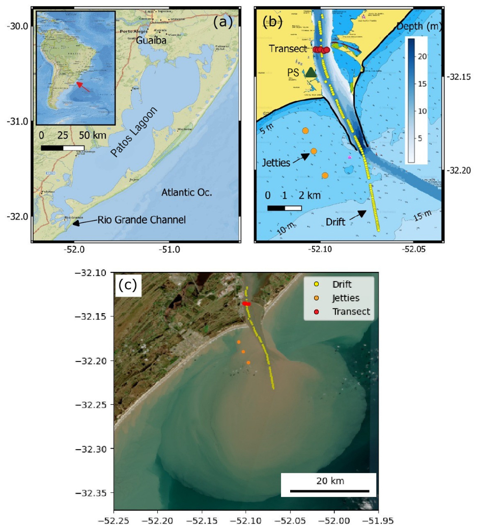
Figure 1 Study area location and sampling design. (a) Regional setting showing the Patos Lagoon choked system and its connection to the South Atlantic Ocean via the Rio Grande Channel. (b) Detailed view of the estuarine–shelf transition; yellow dots represent the Lagrangian track (Drift), orange dots indicate the baseline stations near the breakwaters (Jetties), and red dots show the cross-channel section (Transect). The green triangle (PS) indicates the Rio Grande Pilot Station, the source for meteorological and water level data. Bathymetric contours and the nautical chart emphasize the jetty-constrained morphology. (c) Sampling stations overlaid on a Sentinel-2 true-colour image acquired on 18 July 2022, displaying the turbid surface plume during the survey period. Contains modified Copernicus Sentinel data.

3 Materials and Methods

3.1 Fieldwork Design and Data Collection

The fieldwork was designed to capture the along-channel variability of the vertical structure of current velocities, water properties, and mixing over the transition from the lagoon inlet and channel to the adjacent shelf, and into the buoyant plume beyond the jetties. The survey was conducted on 18 July 2022, coinciding with a Sentinel satellite overpass with clear-sky conditions, enabling a spatial match between in-situ data and the surface extent of the plume (Fig. 1c). During the field survey, outflow currents predominated, consistent with the conditions described in Sect. 2, where inflow and outflow at the mouth are primarily modulated by a subtidal wind-driven regime, with astronomical tides playing a minor role.

Considering the limited influence of astronomical tides in the region, the sampling strategy prioritized spatial coverage over tidal phase, and the field campaign was organized into three segments: thalweg drift (Drift), inner shelf outside the jetties (Jetties), and cross-sectional transect (Transect), as referred to hereafter (Fig 1). The Drift segment collected over ∼ 2 h and 20 min (11:21–13:40 LT) represents the main dataset of the experiment, aiming to capture the longitudinal transition from channelized flow to the early buoyant plume evolution. This segment involved a Lagrangian drift along the thalweg of the channel (with the boat moving passively with the outflow), represented by yellow dots in Fig. 1b and c, totalling 108 microstructure profiles collected over approximately 13 km. While small adjustments were required inside the channel to compensate for wind-induced drag and maintain the boat within the thalweg, no corrections to the track were made once outside the inlet. The microstructure profiles were collected with a Rockland Scientific MicroCTD, which will be elaborated upon later in this section.

Subsequently, two complementary sampling segments were performed to characterize the boundary conditions. The Jetties segment (14:30–14:50 LT) was conducted on the inner shelf adjacent to the jetties (orange dots, Fig. 1b and c) to provide baseline values of TKE dissipation outside the buoyant plume, comprising 17 microstructure profiles across three stations. Finally, the Transect segment (15:45–16:30 LT) consisted of a cross-channel section at the upstream portion of the study area (red dots, Fig. 1b and c). This segment included 26 profiles distributed across five stations (∼ 5 profiles per station), designed to capture cross-channel hydrographic variability and quantify the volume outflow discharge during the survey.

During the Drift, Transect and Jetties sampling, current velocities were recorded concurrently using a vessel-mounted Teledyne RDI Workhorse 1200 kHz Acoustic Doppler Current Profiler (ADCP) operating in bottom-tracking mode. The instrument was configured with a ping interval of 0.5 s and a vertical bin size of 0.25 m, with the first measurement bin located approximately 1.5 m below the water surface. Horizontal positioning was determined via a GPS unit directly connected to the ADCP system, with an estimated positional uncertainty of ∼ 5 m. The ADCP operated continuously throughout the field campaign, providing uninterrupted velocity measurements along the survey track. The total water flow across the transect segment was obtained from direct measurements using an ADCP, processed with the WinRiver II software provided by Teledyne RDI.

Salinity and temperature vertical profiles were recorded with a Rinko Profiler CTD (by JFE Advantech LTD) and with a Conductivity-Temperature Sensor (JAC CT) integrated into a Rockland Scientific microstructure profiler (MicroCTD). The MicroCTD recorded shear by two orthogonally mounted shear probes operating at a sampling rate of 512 Hz. The shear profiles were used to estimate turbulence in terms of TKE dissipation rate (ϵ).

The MicroCTD was deployed a total of 152 times in the downward profiling mode at the locations indicated in Fig. 1b and c, and lowered vertically using a weighted collar to ensure a controlled descent speed of approximately 0.8 m s⁻¹ and an angle of attack below 5° (Lueck, 2013; Lueck et al., 2013; Ross et al., 2019; Barros et al., 2025). The MicroCTD data were georeferenced and synchronized with the ADCP data. For each MicroCTD cast, there is a corresponding vertical profile of horizontal velocities, u and v, time-averaged over a one-minute interval.

Additional environmental data, including wind, water level, and Eulerian current measurements, were obtained from the Rio Grande Pilot Station (Fig. 1b). Wind observations were collected by a Davis Vantage Pro 2 meteorological station, recording at 5 min intervals and averaged hourly. Water level and current velocity were measured with a moored Sontek Argonaut-XR 1.5 MHz ADCP, deployed at approximately 17 m depth. This instrument recorded 5 min averaged profiles with a vertical bin size of 1.5 m.

Estimates of freshwater discharge into the Patos Lagoon were also incorporated, based on daily records from the primary tributaries. Discharge data were retrieved from Brazil's National Water Agency (ANA, 2023) Hidroweb database (http://www.snirh.gov.br/hidroweb, last access: 10 September 2023), using gauge stations from the Jacuí (85900000), Taquari (86720000), Caí (87170000), Sinos (87382000), and Camaquã (87905000) rivers. Additionally, discharge from the São Gonçalo Channel, which connects the Mirim Lagoon to the estuarine system, was provided by the Mirim Lagoon Agency (ALM, 2023). The methodology used to aggregate and estimate river discharge followed the approach described by Santa-Rosa and Schettini (2024).

3.2 Data Analysis

3.2.1 Vessel-mounted ADCP data

The current velocity data recorded by the ADCP were trimmed within 10 % of the bottom to remove erroneous data due to side-lobe effects. Velocities greater than 5 % of the maximum flow were excluded, and any data ensemble with a signal return less than 85 % good data was removed (Ross et al., 2019). Velocity components were rotated via principal component analysis to align with the longitudinal flow direction (Thomson and Emery, 2014). For the data recorded in the channel, the decomposition considered two sectors with relatively similar orientation, up to the inlet. Seaward of the inlet, the currents were decomposed into cross-shelf and along-shelf components based on the coastline orientation, determined by two reference points located approximately 10 km on either side of the jetties.

3.2.2 MicroCTD data

The rate of dissipation (ϵ) of TKE is derived from the measurements of velocity shear recorded by the shear probes on the MicroCTD (Lueck et al., 2020). Assuming that the turbulence is isotropic, the TKE dissipation rate is given by:

$$\begin{array}{}\text{(1)}& \mathit{ϵ}={\displaystyle \frac{\mathrm{15}}{\mathrm{2}}}\mathit{\nu }\stackrel{\mathrm{‾}}{{\left({\displaystyle \frac{\partial u}{\partial z}}\right)}^{\mathrm{2}}}={\displaystyle \frac{\mathrm{15}}{\mathrm{2}}}\mathit{\nu }{\int }_{\mathrm{0}}^{\mathrm{\infty }}\mathrm{\Psi }\left(k\right)\mathrm{d}k,\end{array}$$

where ν is the kinematic molecular viscosity (10⁻⁶ m² s⁻¹), Ψ is the velocity shear spectrum, and k is the wave number (m⁻¹) (Lueck, 2013). This ϵ is expressed as the rate of dissipation of TKE per unit mass (W kg⁻¹, or equally, m² s⁻³) (Thorpe, 2007).

The estimates of ϵ from the two independent shear probes were compared at each depth and when the value differed by more than a factor of two, the larger estimate was discarded following quality-control procedure by Stips (2005). Only two vertical profiles were discarded due to deviations from the operational thresholds of the angle of attack being more than 5° or the descent speed deviating from 0.8 m s⁻¹, representing less than 1.3 % of the total casts. Correction for profiler vibration was made using the method of Goodman et al. (2006). Individual wave number spectra for each component were calculated using a Fast Fourier Transform (FFT) with a length of 0.5 m and a time span of 2 s for each estimate of the rate of dissipation. Both calculated ϵ data sets were averaged and then used to quantify the vertical eddy viscosity (A_z). The calculations were done using the Matlab scripts provided by Rockland Scientific, and further pre-processed with Python (Schettini, 2021). Subsequently, all turbulence analysis and the computation of dimensionless stability metrics were performed using a dedicated Python codebase developed for this study (Barros, 2026). This secondary processing stage ensures the reproducibility of the mixing estimates and hydraulic parameters presented hereafter.

3.2.3 Turbulence Parameters and Vertical Mixing

To estimate vertical eddy viscosity (A_z) as a proxy for vertical mixing, the following procedure was adopted. First, along-channel and cross-channel velocity components from each transect were used to calculate the squared vertical shear (S²), defined as:

$$\begin{array}{}\text{(2)}& S^{\mathrm{2}}={\left({\displaystyle \frac{\partial u}{\partial z}}\right)}^{\mathrm{2}}+{\left({\displaystyle \frac{\partial v}{\partial z}}\right)}^{\mathrm{2}},\end{array}$$

where u and v are the longitudinal and lateral flow components, respectively, and the coordinate z is positive upward. The buoyancy frequency (N²) was used to estimate the stratification and is quantified as:

$$\begin{array}{}\text{(3)}& N^{\mathrm{2}}=-{\displaystyle \frac{g}{{\mathit{\rho }}_{\mathrm{o}}}}{\displaystyle \frac{\partial \mathit{\rho }}{\partial z}},\end{array}$$

where g is the gravitational acceleration (9.8 m s⁻²), and ρ_o is a reference density (1025 kg m⁻³). The stratification stability parameter, also known as the dimensionless gradient Richardson number, is expressed as the ratio of buoyancy frequency to squared vertical shear, $\mathit{Ri}=N^{\mathrm{2}}/S^{\mathrm{2}}$, and was calculated to quantify the influence of stratification on mixing (Monismith, 2010).

From Ri, the flux Richardson number was obtained as a scale for mixing efficiency (Holleman et al., 2016; Gregg et al., 2018), representing the ratio of buoyancy to production. Following Venayagamoorthy and Koseff (2016) it can be expressed as:

$$\begin{array}{}\text{(4)}& R_{\mathrm{f}}=\mathrm{0.25}\left(\mathrm{1}-e^{-\mathrm{7}{R}_{\mathrm{i}}}\right).\end{array}$$

According to Kay and Jay (2003), in stable stratified flow, R_f is the fraction of total TKE production that is lost to buoyancy, increasing the potential energy of the water column, typically bounding toward an upper limit of 0.25. The mixing coefficient Γ_m is denoted by the mixing efficiency R_f.

$$\begin{array}{}\text{(5)}& {\mathrm{\Gamma }}_{\mathrm{m}}={\displaystyle \frac{R_{\mathrm{f}}}{\mathrm{1}-R_{\mathrm{f}}}}.\end{array}$$

The vertical eddy viscosity, a proxy of mixing, was calculated using the mixing efficiency as follows (Kay and Jay, 2003; Huguenard et al., 2015; Ross et al., 2019):

$$\begin{array}{}\text{(6)}& A_z={\mathrm{\Gamma }}_{\mathrm{m}}{\displaystyle \frac{\mathit{ϵ}}{S^{\mathrm{2}}}}.\end{array}$$

The buoyancy Reynolds number, Re_b, is a parameter used to indicate the impact of density stratification on turbulence (Stacey et al., 1999; Shih et al., 2005; Monismith, 2010; Holleman et al., 2016; Barros et al., 2025). It is calculated as:

$$\begin{array}{}\text{(7)}& {\mathit{Re}}_{\mathrm{b}}={\left({\displaystyle \frac{L_{\mathrm{o}}}{L_{\mathrm{k}}}}\right)}^{\mathrm{4}/\mathrm{3}}={\displaystyle \frac{\mathit{ϵ}}{\mathit{\nu }{N}^{\mathrm{2}}}}\end{array}$$

where the $L_{\mathrm{o}}/L_{\mathrm{k}}$ is the ratio between the Ozmidov length scale and the Kolmogorov length scale (larger scale over smaller scale of turbulence). The magnitude of Re_b defines distinct regimes in the interaction between buoyancy and turbulence: for Re_b > 200, small-scale turbulence is unaffected by stratification; for 15 < Re_b < 200, the effect of stratification progressively extends to smaller and smaller scales; and for Re_b < 15, stratification becomes dominant, resulting in the complete suppression of turbulence (a phenomenon often referred to as “killing turbulence”) (Gargett et al., 1984; Ivey et al., 2008; Monismith, 2010).

3.2.4 Internal Froude Number Calculation

The internal Froude number (Fr_i) is a dimensionless measure of the ratio between inertial and buoyancy forces. It was calculated following (Hetland, 2010; McPherson et al., 2020):

$$\begin{array}{}\text{(8)}& {\mathit{Fr}}_{\mathrm{i}}={\displaystyle \frac{\mathrm{\Delta }U}{\sqrt{g^{\prime }h}}}\end{array}$$

where $\mathrm{\Delta }U=U_{\mathrm{1}}-U_{\mathrm{2}}$ is the velocity difference between the upper and the lower layer, and h is the thickness of the low-density surface layer. The term $\sqrt{g^{\prime }h}$ represents the internal wave speed, where g^′ is the reduced gravity, defined as $g^{\prime }=g(\mathrm{\Delta }\mathit{\rho }/{\mathit{\rho }}_{\mathrm{0}})$, where $\mathrm{\Delta }\mathit{\rho }={\mathit{\rho }}_{\mathrm{2}}-{\mathit{\rho }}_{\mathrm{1}}$, is the density difference across the interface as a function of depth.

Determining h requires identifying the pycnocline depth. Within the channel, this was defined by the maximum vertical density gradient ($\partial \mathit{\rho }/\partial$z) for each density profile. The density structure in this region was generally characterized by a well-defined two-layer system, allowing the interface depth to be objectively identified using this criterion.

In the offshore region, however, the strongest vertical density gradient often occurred within the upper portion of the buoyant plume rather than at its base. As a result, applying the maximum-gradient criterion offshore frequently produced unrealistically shallow interface depths that underestimated the effective thickness of the surface plume layer relevant to the hydraulic analysis. The upper layer thickness in the offshore profiles was determined using a profile-shape criterion, defined as the depth at which the density profile transitions from a strongly stratified upper layer (plume) to a nearly homogeneous underlying water mass (coastal water). This transition was identified from the inflection region of each density profile, corresponding to the point where the sharp density gradient of the surface plume gives way to a nearly uniform deeper layer (Fig. 6). This approach identifies the base of the buoyant plume while avoiding spurious detection of near-surface gradients.

Because the vertical density structure differs substantially between the confined channel and the offshore plume region, different interface definitions were required to consistently represent the upper-layer thickness across the channel-to-shelf transition. Although alternative interface definitions would modify values of Fr_i, the adopted methodology provides a physically meaningful estimate of the buoyant layer thickness and supports the interpretation of the observed spatial patterns in flow regime.

Subcritical flow (Fr_i < 1) indicates buoyancy-dominated conditions where internal waves can propagate upstream and the plume tends to be stable and spreads horizontally, whereas supercritical flow (Fr_i > 1) indicates inertia-dominated conditions, where stratification is insufficient to constrain the flow, potentially leading to enhanced turbulent mixing (Nash and Moum, 2005; Hetland, 2010; Horner-Devine et al., 2015; Geyer et al., 2017).

3.2.5 Channel Morphology

In order to understand the influence of channel morphology on the measured and derived variables, cross-sectional areas along the channel were calculated. The inner channel was divided into 57 cross-sections, and the area of each section was estimated by constructing a closed polygon bounded above by the water surface and below by a high-resolution bathymetric survey conducted in 2024 using a single-beam echosounder and DGPS positioning (Fig. 1b).

For each section, a reference line was defined between two control points, and all bathymetric data within a lateral buffer of ±50 m from this line were considered. To project the bathymetric points onto the local reference frame of the transect, each point (x,y) was expressed in terms of its longitudinal (d_∥) and perpendicular (d_⟂) distances:

$$\begin{array}{}\text{(9)}& {\displaystyle }{d}_{\parallel }=\left(x-x_{\mathrm{0}}\right)u_x+\left(y-y_{\mathrm{0}}\right)u_y\text{(10)}& {\displaystyle }{d}_{⟂}=\left|\left(x-x_{\mathrm{0}}\right)\left(-u_y\right)+\left(y-y_{\mathrm{0}}\right)u_x\right|\end{array}$$

where (x₀, y₀) is the starting point of the transect, and (u_x,u_y) is the unit vector in the direction of the transect. Points satisfying 0 ≤ $d_{\parallel }\le$ L and $d_{⟂}<\mathrm{50}$ m (with L being the transect length) were retained for area calculation.

The bathymetric profile was ordered along the transect axis to form the lower boundary of the polygon, while the water surface was assumed to be locally horizontal and defined by a straight line between the transect endpoints. This assumption is reasonable for short cross-sections and allows the area to represent a first-order approximation of the wet section at the time of sampling. The polygon was constructed by concatenating the surface line with the reversed bathymetric profile.

4 Results

4.1 Environmental Conditions and Inner Channel Dynamics (The Transect Segment)

The environmental conditions during the survey favoured the outflow of lagoon waters and the formation of a buoyant plume. To characterize this state, the river discharge of the main tributaries, along with water level, wind vectors in meteorological convention, and current velocities measured in the channel at the Pilot's Station (Fig. 1b) during the days preceding the survey, are shown in Fig. 2. On the day of the fieldwork (18 July 2022), the gauged river discharge was approximately 6900 m³ s⁻¹ (Fig. 2a), which is significantly higher than the estimated average flow of 3707 m³ s⁻¹ for the same month. Importantly, elevated discharge conditions had persisted for several days prior to the survey, indicating sustained freshwater forcing rather than a transient increase in river discharge.

The gauged river discharge represents the freshwater inflow to the lagoon measured upstream from any coastal sea level influence in fully freshwater sections of the main tributaries. However, it does not necessarily correspond to the discharge at the lagoon mouth due to storage, mixing, and exchange processes within the lagoon (Santa-Rosa and Schettini, 2024). The total discharge at the lagoon mouth, measured across the Transect segment, reached 9400 m³ s⁻¹, with an average salinity of 6 g kg⁻¹ (Fig. 3b). Using the observed coastal salinity during the survey (∼ 28 g kg⁻¹) as a reference, the freshwater discharge was estimated at 7650 m³ s⁻¹. The difference between the gauged river discharge and the actual freshwater flow at the lagoon's mouth can be attributed to wind-driven water level variations along the lagoon and the residence time of water parcels within the system.

Water level variability during the survey was minimal, fluctuating by approximately 0.20 m (Fig. 2b). Wind speeds were relatively weak compared to the preceding days (Fig. 2c), blowing from NNW to W and ranging between 1.8 and 5.4 m s⁻¹. The current flowed seaward throughout the entire water column during the fieldwork (Fig. 2d), with velocities ranging from 0.8 m s⁻¹ near the bottom to 2.2 m s⁻¹ near the surface, without reversal. These results from the moored ADCP corroborate the Transect observations (Fig. 3a), showing outflow across the entire water column, with higher velocities of approximately 2 m s⁻¹ concentrated at the surface and along the main axis of the channel.

Together, the elevated river discharge, weak water-level variability, and persistent ebb-directed flow indicate that the system was not responding to tidal oscillations but rather to sustained subtidal forcing acting over several days. Such prolonged forcing conditions are characteristic of microtidal environments and allow the estuary–plume system to evolve toward a quasi-steady state.

Nevertheless, this condition represented a significant variation compared to the previous days in the interval, during which the current had been flowing in the opposite direction due to the passage of a frontal system with up-estuary winds. Following the relaxation of those winds, the system rapidly re-established a persistent seaward-directed circulation that remained stable for several days and throughout the survey period. This high-discharge, outflow-dominated state provides the boundary conditions for the plume development analysed in the following section.

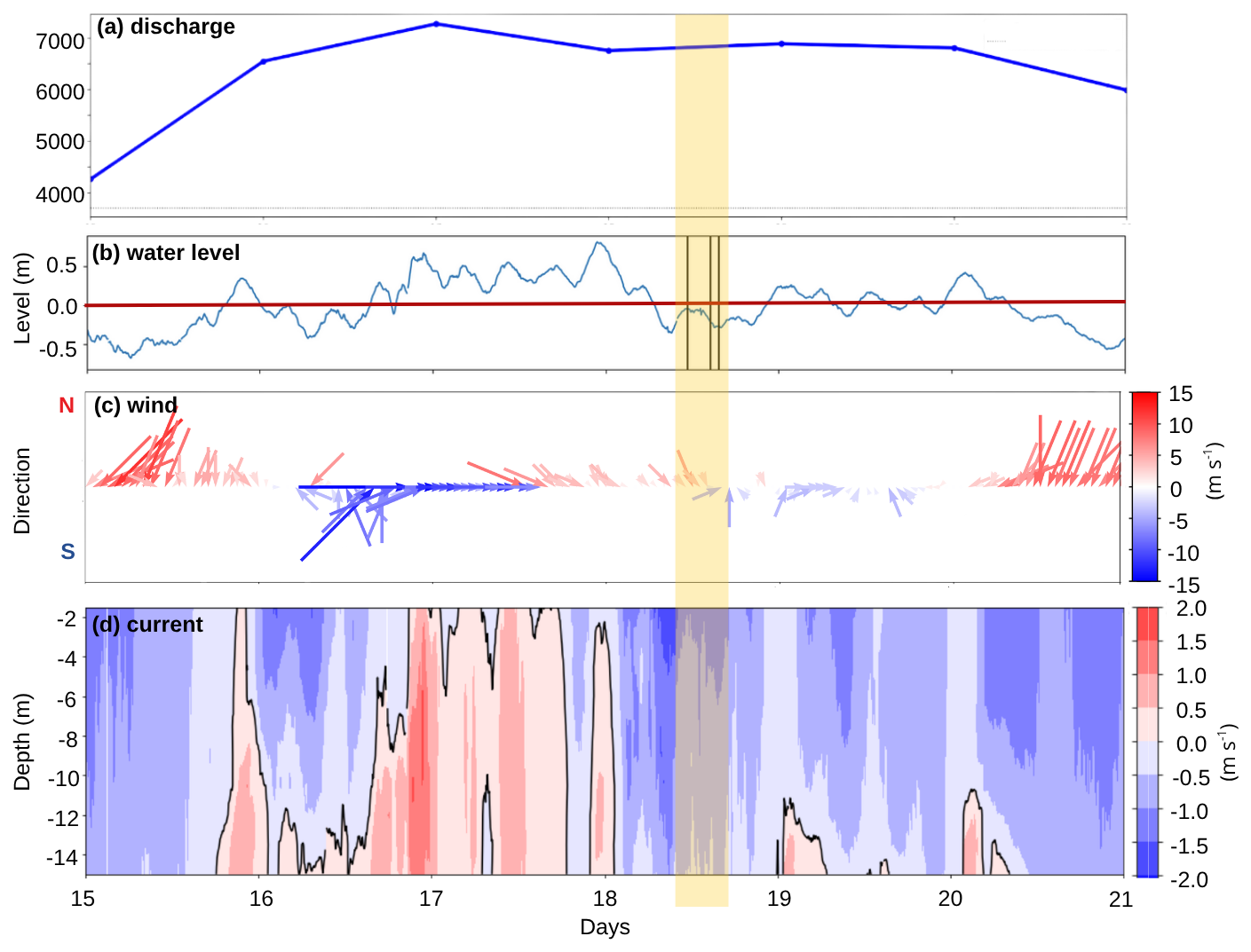
Figure 2 Environmental conditions between 15 and 21 July 2022, with the vertical yellow bar representing the survey period. (a) Gauged river discharge of the Patos Lagoon (m³ s⁻¹). (b) Water level (m) measured in the channel, where the three vertical lines indicate the start moment of each section: Drift, Jetties, and Transect. (c) Vector plot of wind velocity (m s⁻¹) in meteorological notation, where blue represents southerly winds (blowing towards the north) and red represents northerly winds (blowing towards the south). (d) Hovmöller diagram of the along-channel current velocity (m s⁻¹) measured in the channel, where red indicates inflow (flood) and blue indicates outflow (ebb).

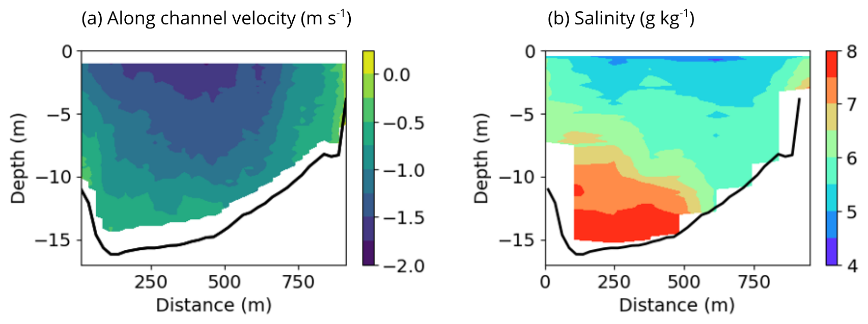
Figure 3 Cross-sectional distribution of (a) along channel current velocity (m s⁻¹; negative values indicate outflow) and (b) salinity (g kg⁻¹) at the Transect segment, characterizing the lagoon outflow during the survey.

4.2 Estuary–Shelf Transition and Near-Field Plume (The Drift Segment)

The spatial distributions along the Drift segment are presented in scatter plot diagrams, where vertical profiles feature a 0.5 m resolution and horizontal positioning corresponds to each cast's location. This graphical representation underscores the extensive sampling density achieved during the campaign and allows for the identification of spatial coherence between neighbouring profiles. Such high-resolution visualization is particularly relevant for properties with strong spatial variability, such as TKE dissipation (ϵ) and the Richardson number (Ri), ensuring that the observed structures reflect genuine physical features captured at the sampling sites.

4.2.1 Water Mass Characterization and Vertical Structure

The spatial distribution of temperature, salinity, and density across the Drift segment illustrates the horizontal and vertical development of the estuarine plume as it exits the channel. Within the channel (distance ≤ ∼ 8.5 km), salinity (Fig. 4a) ranged from 7 to 13 g kg⁻¹, with a relatively clear vertical distinction at the density interface (black dashed line in Fig. 4a–c). In the outer region (distance ≥ ∼ 8.5 km), vertical variability intensifies, with values spanning 7 to 28 g kg⁻¹ near the mouth, followed by a gradual increase in surface salinity as the plume disperses offshore. Temperature (Fig. 4b) shows less variability than salinity (< 1 °C) but remains consistent with salinity patterns. Consequently, the density distribution (Fig. 4c) closely mirrors salinity, ranging from 1005 to 1021 kg m⁻³.

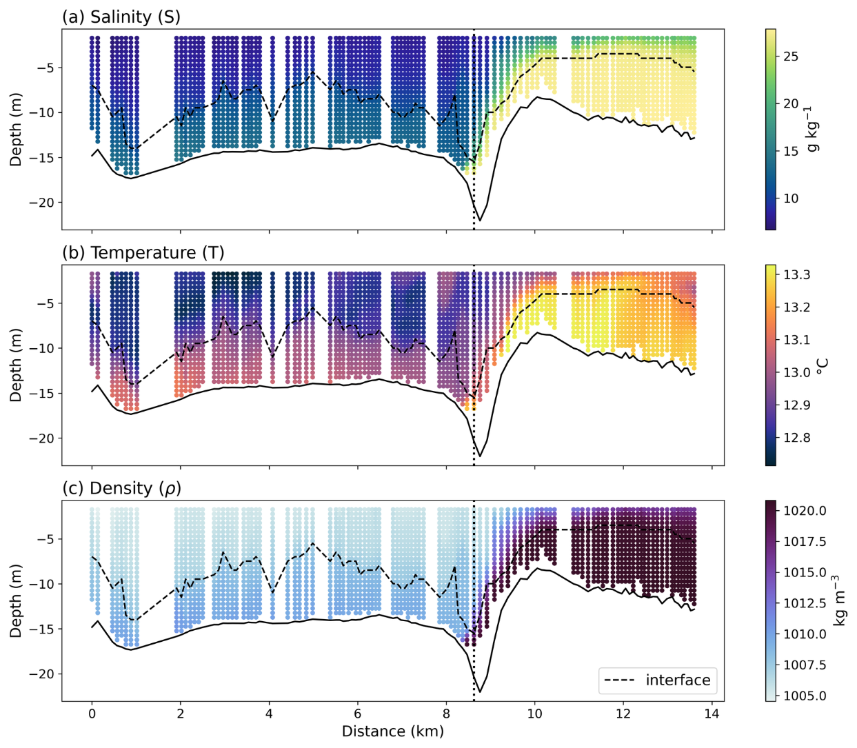
Figure 4 Spatial distributions of (a) salinity (g kg⁻¹), (b) temperature (°C), and (c) density (kg m⁻³). The dashed line indicates the interface position between layers. The vertical dotted line marks the position of the mouth (inlet). Distance (km) is measured from the first upstream profile within the channel.

The transition from the laterally constrained channel flow to the unconstrained shelf environment is marked by significant morphological changes and baroclinic adjustments (Chao and Boicourt, 1986; Valle-Levinson et al., 1996). The T–S diagram (Fig. 5) illustrates the thermohaline structure resulting from these adjustments and the subsequent mixing stages of the sampled waters, distinguishing the inner region (warm tones) from the outer region (cold tones), with colour shading indicating depth. The distribution reveals three primary water masses: (i) low-salinity (< 15 g kg⁻¹), representing estuarine water influenced by river discharge and meteorological forcing; (ii) an intermediate salinity range (15–27 g kg⁻¹), reflecting active mixing between estuarine and coastal waters; and (iii) high-salinity (> 27 g kg⁻¹), representing relatively homogeneous coastal water.

The low-salinity partially mixed estuarine water (< 15 g kg⁻¹) is composed of two main branches: the first with a vertical shape (yellow, with salinity < 8 g kg⁻¹) represents near-surface estuarine water, while the second (red, with salinity ranging from 8–15 g kg⁻¹) exhibits a diagonal trend, representing the deeper estuarine layer. These two branches indicate the coexistence of distinct surface and deeper estuarine waters within the channel, supporting the interpretation of a vertically stratified water column prior to plume detachment at the mouth.

The intermediate mixing region (majority of blue points, 15–27 g kg⁻¹), shows the data also along a well-defined diagonal trend, reflecting coupled variations in temperature and salinity and thus active conservative mixing between estuarine and coastal waters, representing the plume waters over the shelf.

At higher salinities, the distribution becomes more vertically clustered again (purple cluster, > 27 g kg⁻¹), representing a second, relatively homogeneous water mass associated with coastal waters. This most saline and deeper water represents the regional coastal water under the influence of the La Plata River plume, a buoyant coastal current that flows northward along the southwestern Atlantic shelf and episodically reaches the study area, modulating the thermohaline structure of the adjacent coastal waters, particularly during winter (Campos et al., 2008).

The geometry of these branches indicates the nature of the mixing processes (Miranda et al., 2002). Additionally, the marginal histograms (Fig. 5) highlight the sampling density, where the bimodal salinity distribution underscores the clear separation between the estuarine core and the coastal water. In contrast, the more continuous temperature distribution, given its relatively small range (∼ 0.6 °C) reflects the subtle thermal gradient across the plume, confirming that density remains primarily salinity-driven in this near-field region.

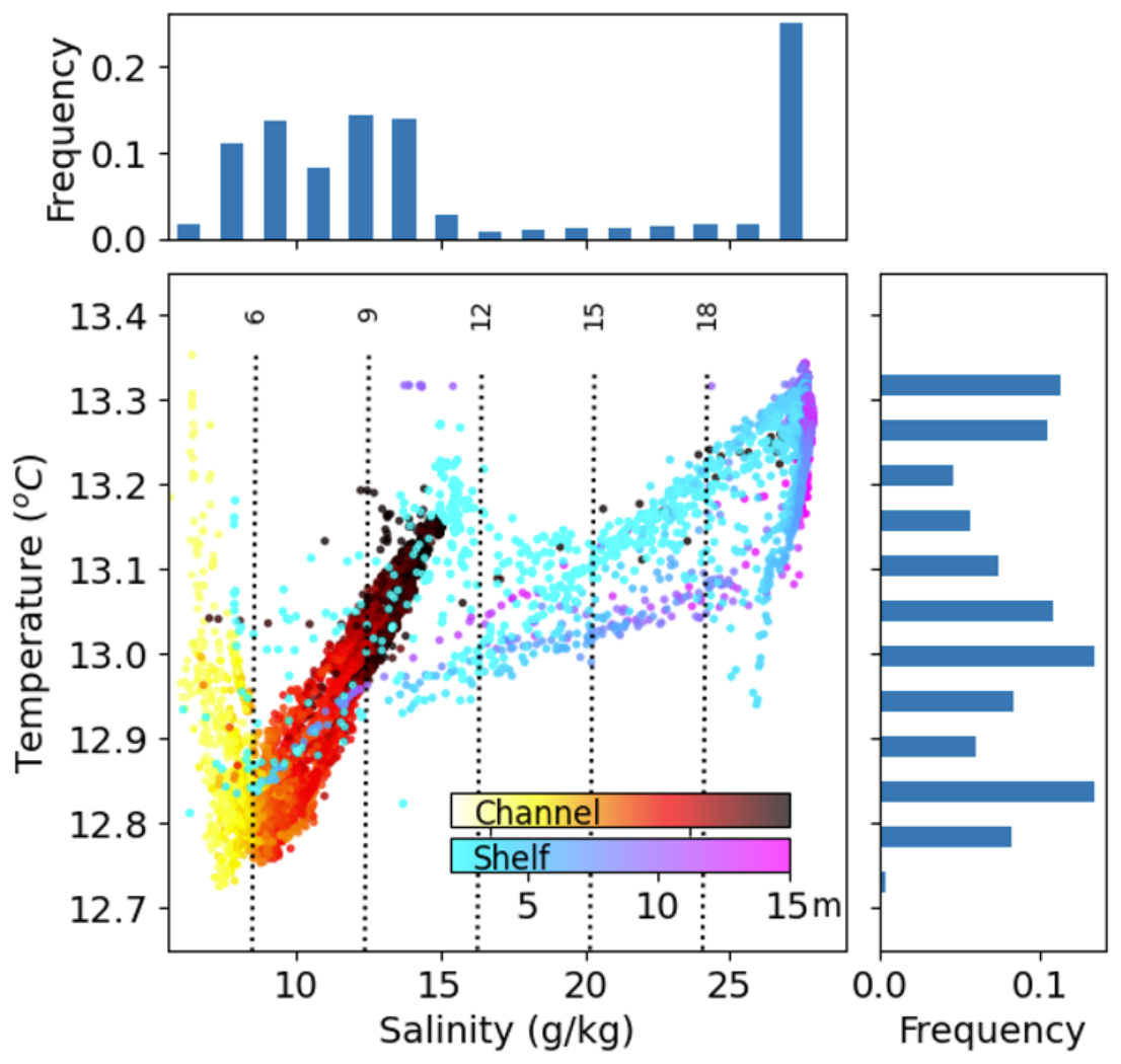
Figure 5 Temperature–Salinity (T–S) diagram and frequency histograms of salinity (top) and temperature (right) for the Drift segment. The central panel shows temperature (°C) versus salinity (g kg⁻¹), with dotted vertical lines indicating density anomaly (σ_t) values. The colour bar distinguishes data from the Channel (warm tones) and the Shelf (cold tones), with shading representing the sampling depth (m).

The high-resolution vertical density profiles exhibit the structural evolution of the water column across the channel-to-shelf transition (Fig. 6). Within the channel (red-toned lines), profiles are clustered between 1005 and 1010 kg m⁻³, with relatively weak vertical density gradients, especially when compared to other conditions in the same system (Barros et al., 2025), indicating a partially mixed water column. As the flow exits the jetties into the shelf (blue-toned lines), a sharp two-layer stratification emerges. In this outer region, surface density increases to 1012–1021 kg m⁻3, while the pycnocline rises and stabilizes at depths shallower than 5 m. Below this interface, density converges to values between 1020 and 1021 kg m⁻³. This transition from a less stratified channel flow to a more strongly stratified near-field plume provides the physical context for the flow and mixing results presented next.

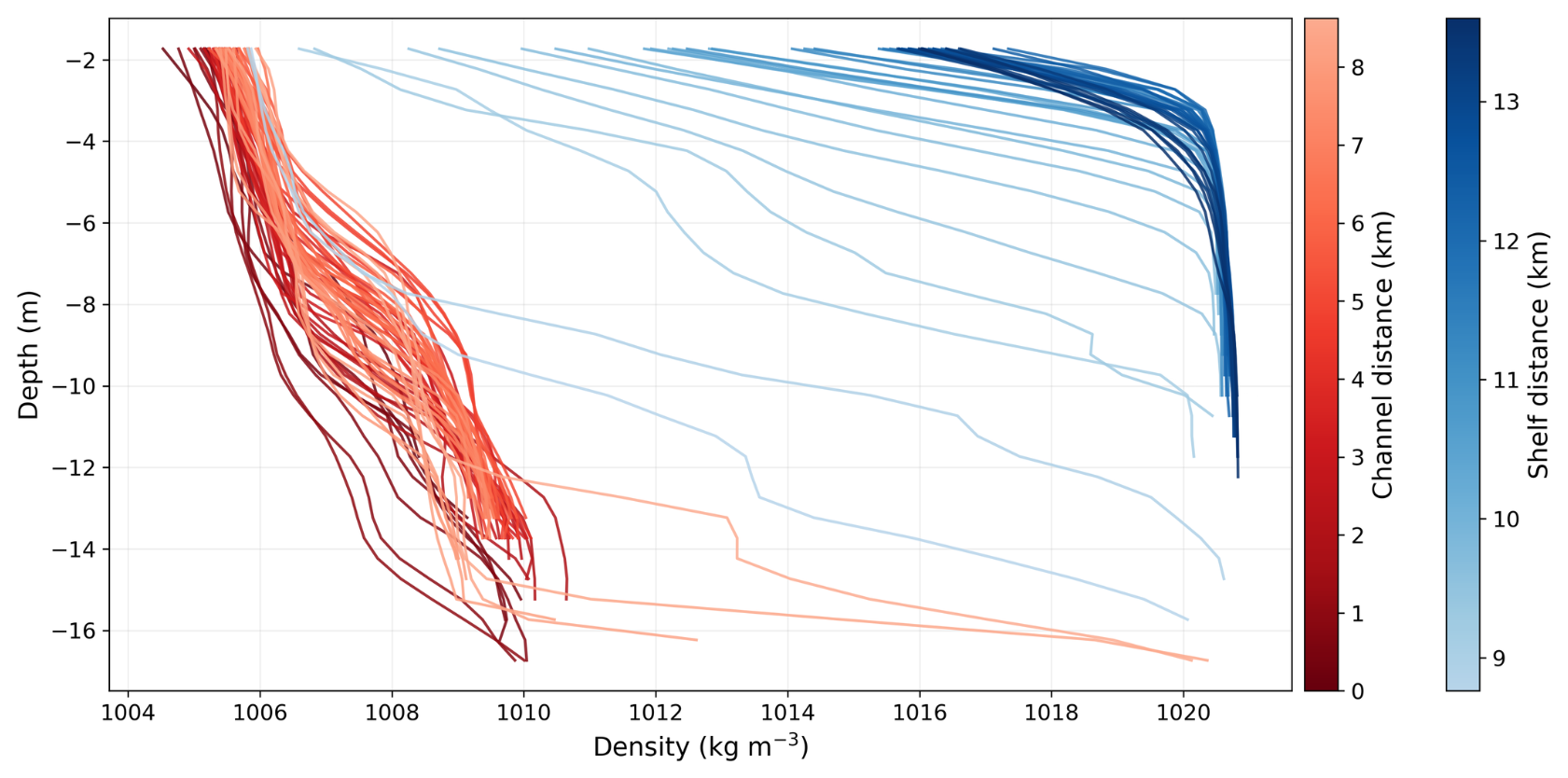
Figure 6 Vertical density profiles (kg m⁻³) across the channel-to-shelf transition. Lines are colour-coded by distance (km) from the starting point of the drift segment. Red tones represent profiles within the inner channel (0–8.5 km) and blue tones represent profiles in the shelf region (9–13.5 km).

4.2.2 Flow Dynamics and Velocity Structure

The longitudinal velocity component (Fig. 7a) shows a predominantly seaward-directed (negative) flow throughout the entire water column, with higher velocities at the surface (up to ∼ 1.8 m s⁻¹) that decrease with depth. A vertical gradient of the along-channel velocity occurs at the interface between the two density layers, indicated by the dashed line in Fig. 7a. Although this observation is subtle in the velocity data alone, it becomes more evident when viewed alongside the water property observations (Fig. 4). However, beyond the inlet (km 8.5), this vertical gradient becomes more pronounced. The intensity of the outflow in the upper layer intensifies, exceeding 2.0 m s⁻¹ just after the mouth at the estuary–ocean connection. The upper layer loses momentum as its thickness increases farther offshore (beyond km 11), while moving away from the source region. Below the interface, the velocity is significantly lower (typically < 0.5 m s⁻¹, representing less than 25 % of the surface magnitude) and a flow reversal (positive values) occurs near the bottom in the outermost portion.

The cross-channel velocity component (Fig. 7b) within the inner channel exhibits magnitudes ranging from −0.51 to 0.41 m s⁻¹, reflecting a flow primarily aligned with the longitudinal axis. These lateral flow patterns change direction (shifting between positive and negative values) across the water column, especially along the layer interface, particularly in the region of highest constriction (approx. km 8). Once on the shelf (beyond km 9), the cross-shelf signal becomes dominant, reaching magnitudes of −0.68 m s⁻¹ and showing consistency throughout the water column. This shift reflects that, once outside the channel's confinement, the plume's lateral flow responds mainly to shelf forcing, whereas the inner channel circulation reflects local morphological adjustments.

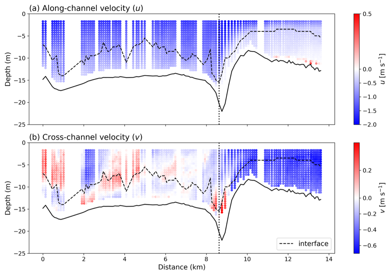
Figure 7 Spatial distributions of (a) along-channel and (b) cross-channel velocity components (m s⁻¹) synchronized with the MicroCTD profiles. The dashed line indicates the interface position between layers. The vertical dotted line marks the position of the mouth (inlet). Distance (km) is measured from the first upstream profile within the channel.

4.2.3 Turbulent Regimes and Stability Parameters

The turbulent kinetic energy dissipation rate (ϵ) along the section is presented in Fig. 8. The values of ϵ vary across four orders of magnitude, ranging from 10⁻⁷ to 10⁻³ W kg⁻¹. The highest values were recorded in the region immediately following the mouth (km 9–10) throughout the entire water column. This zone of high dissipation extends offshore within the surface layer above the interface. Below the interface on the shelf, dissipation values were relatively lower (10⁻⁶ W kg⁻¹). The lowest just after the mouth and the dissipation values (< 10⁻⁷ W kg⁻¹) were recorded within the channel in the mid-water column between km 5 and 7, in the vicinity of the density interface. This zone corresponds to the wider section that precedes the narrowing of the jetties towards the mouth.

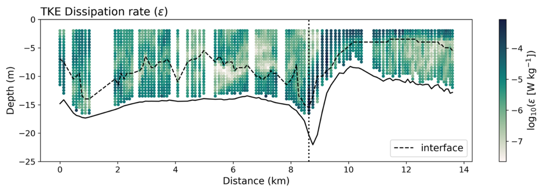
Figure 8 Spatial distribution of the turbulent kinetic energy dissipation rate (ϵ, log₁₀(W kg⁻¹)). The dashed line indicates the interface position between layers. The vertical dotted line marks the position of the mouth (inlet). Distance (km) is measured from the first upstream profile within the channel.

The spatial distributions of buoyancy frequency (N²) and squared vertical shear (S²), and the gradient Richardson (Ri) are presented in Fig. 9. The buoyancy frequency (Fig. 9a) shows lower variability along the channel, with higher values coinciding with the pycnocline (interface). On the shelf, a more intense vertical gradient is observed between the surface layer, presenting higher values (∼ 10⁻¹ s⁻²), and the bottom layer (∼ 10⁻⁵ s⁻²). The spatial distribution of the squared vertical shear (Fig. 9b) is relatively consistent with the N² patterns. The highest S² values also occur at the transition between the inlet and the shelf, as well as within the shelf's surface layer (∼ 10⁻¹ s⁻²). The largest S² values in the channel were co-located with the pycnocline.

The gradient Richardson number, Ri, was rescaled as log₁₀($\mathit{Ri}/\mathrm{0.25}$), such that positive values reflect Ri > 0.25 and negative values reflect Ri < 0.25 (Fig. 9c), where Ri ≈ 0.25 represents a classical threshold below which stratified shear flows become susceptible to instability (Miles, 1961). Within the inner region of the inlet, values below 0.25 are predominantly concentrated in the surface layer, while values above this threshold occur especially around the interface. Near the mouth (vicinity of km 8.5), nearly the entire water column exhibits values above 0.25, forming a stable vertical barrier. In the outer region, a vertical decoupling is observed where the surface plume and the near-bottom layer present values below 0.25, whereas a persistent layer of values above 0.25 follow the stratified interface region, effectively isolating the plume from the deeper shelf waters.

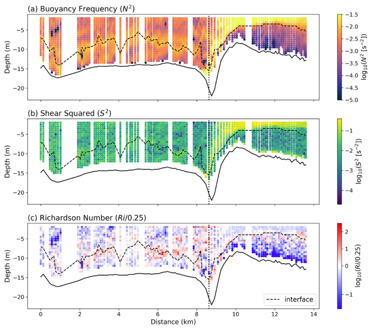
Figure 9 Spatial distributions of (a) buoyancy frequency (N², s⁻²), (b) squared vertical shear (S², s⁻²), and (c) gradient Richardson number normalized by its critical value ($\mathit{Ri}/\mathrm{0.25}$). The dashed line indicates the interface position between layers. The vertical dotted line marks the position of the mouth (inlet). Distance (km) is measured from the first upstream profile within the channel.

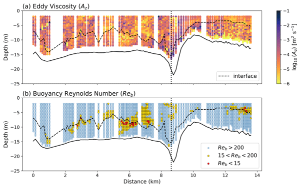
The spatial distributions of the vertical eddy viscosity (A_z) and the buoyancy Reynolds number (Re_b) are presented in Fig. 10. The vertical eddy viscosity exhibits values ranging from 10⁻⁶ to 10⁻¹ m² s⁻¹, showing significant vertical and longitudinal variability along the section (Fig. 10a). The lowest values occur primarily in the mid-water column between km 5 and 7. In contrast, the highest values are found near the seabed on the shelf, adjacent to the mouth at km 9.

The buoyancy Reynolds number was calculated as an indicator of the degree to which stratification suppresses turbulence. High Re_b values are observed throughout most of the channel (Fig. 10b), particularly in the region between km 9 and 10, where values remain above 200 over the water column. Values between 15 and 200, which indicate that stratification is actively constraining turbulence, are specifically found in the mid-water column between km 5 and 7.5, as well as along the density interface in the channel, and near the offshore end of the section (km 13). Values lower than 15 appear at isolated points along the interface, with a notable cluster occurring within the pycnocline between km 5 and 7.5, which indicate that stratification is fully suppressing turbulence at these locations.

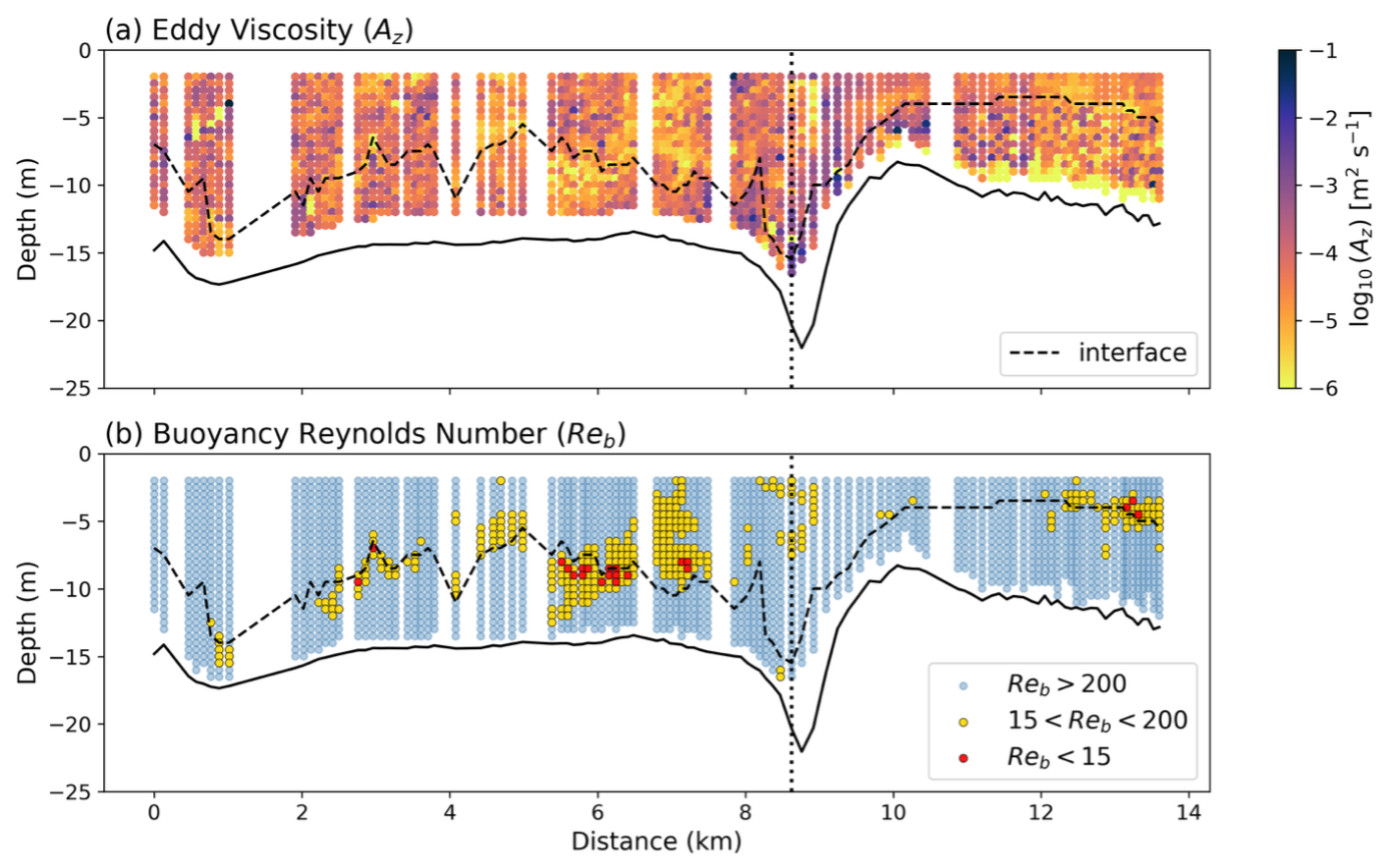
Figure 10 Spatial distributions of (a) the vertical eddy viscosity (A_z, m² s⁻¹), and (b) the buoyancy Reynolds number (Re_b). The dashed line indicates the interface position between layers. The vertical dotted line marks the position of the mouth (inlet). Distance (km) is measured from the first upstream profile within the channel.

4.3 Baseline Inner-Shelf Conditions (the Jetties Segment)

To contextualize the magnitude of the turbulence observed within the plume, the vertical profiles conducted in the Jetties segment serve as a baseline reference for the adjacent inner shelf. Compared to the high-velocity jet observed in the Drift segment, the current velocity profiles at the Jetties segment (Fig. 11a) exhibit distinctly lower magnitudes and greater vertical uniformity, averaging to approximately 0.2 m s⁻¹. Nevertheless, the upper layer at Station 1 (green line), which is the outermost (most seaward) location, exhibited larger variations, reaching over 0.4 m s⁻¹ at the surface. This behaviour is consistent with the density profiles (Fig. 11b), which indicate a more stratified water column at Station 1 compared to moderate stratification at Station 2 (blue line). Conversely, Station 3 (yellow line), which is located closest to shore, exhibits a nearly vertical density profile, indicating a well-mixed water column with no apparent pycnocline.

Under these conditions, the TKE dissipation rates (ϵ) at these stations (Fig. 11c) are significantly lower than those recorded in the main plume axis, ranging between 10⁻⁸ and 10⁻⁶ W kg⁻¹, with the minimum values occurring mid-water column, just below the pycnocline at each station. This is even the case for station 3, which has a nearly uniform density profile, although the values of ϵ are up to a magnitude smaller than the other two stations. Furthermore, A_z fluctuates between 10⁻⁵ and 10⁻³ m² s⁻¹ without a specific vertical pattern (Fig. 11d). The reduced velocities and relative uniformity, combined with the markedly lower stratification and dissipation at these reference points, confirm that the intense turbulent activity described in the Drift segment is an intrinsic process of the plume dynamics rather than a general characteristic of the inner shelf. This contrast highlights the unique turbulent signature of the plume, where internal structures are governed by localized mixing processes at the estuary–shelf interface.

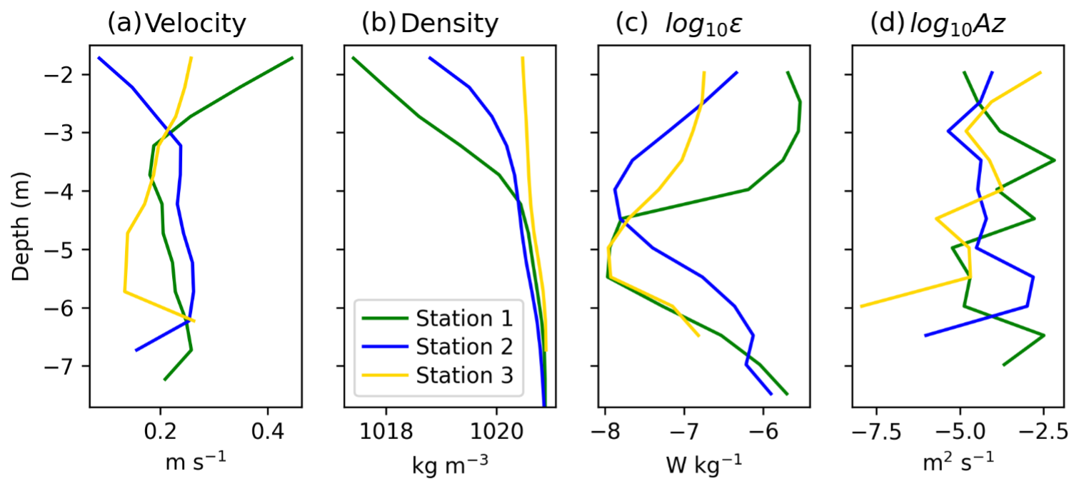
Figure 11 Vertical profiles of (a) current velocity (u, m s⁻¹), (b) water density (ρ, kg m⁻³), (c) TKE dissipation rate (ϵ, W kg⁻¹), and (d) vertical eddy viscosity (A_z, m² s⁻¹) at the three baseline stations in the Jetties segment. Green, blue, and yellow lines represent Stations 1 (outermost), 2 (intermediate), and 3 (innermost), respectively. The x-axis tick labels in panels (c) and (d) indicate the logarithmic exponents.

5 Discussion

5.1 Representativeness of the Sampled Hydrodynamic Conditions

The field campaign spanned approximately 5 h, yet the observations can be interpreted as a quasi-synoptic snapshot of the hydrodynamic conditions. In estuarine environments where astronomical tides are dominant, sampling designs must strictly adhere to hourly variations to capture tidal phases (Dyer, 1979; Kjerfve, 1990). However, in the Rio Grande Channel, astronomical tides play a secondary role, accounting for less than 20 % of the current variance (Santa-Rosa and Schettini, 2024). As established by the spectral characterization for July 2022 (Barros et al., 2025), the system is dominated by low-frequency energy (periods > 25 h) associated with synoptic frontal systems.

This meteorological dominance ensured a quasi-steady state during the survey, characterized by minimal water level fluctuations (< 0.20 m; Fig. 2b) and a persistent, uniform ebb-directed flow (Fig. 2d). Such stationarity validates the comparison of data across different sampling moments, allowing the analysis to move beyond temporal variability and focus on the spatial processes and internal plume structure that define the estuary-shelf transition. To further assess the representativeness of the sampled conditions, the field observations were compared with the annual wind–flow regime space derived from 2022 observations (Fig. 12). Together, these analyses indicate that the field campaign sampled a representative quasi-steady outflow state, providing a robust basis for interpreting the spatial structure and mixing dynamics across the estuary–plume transition.

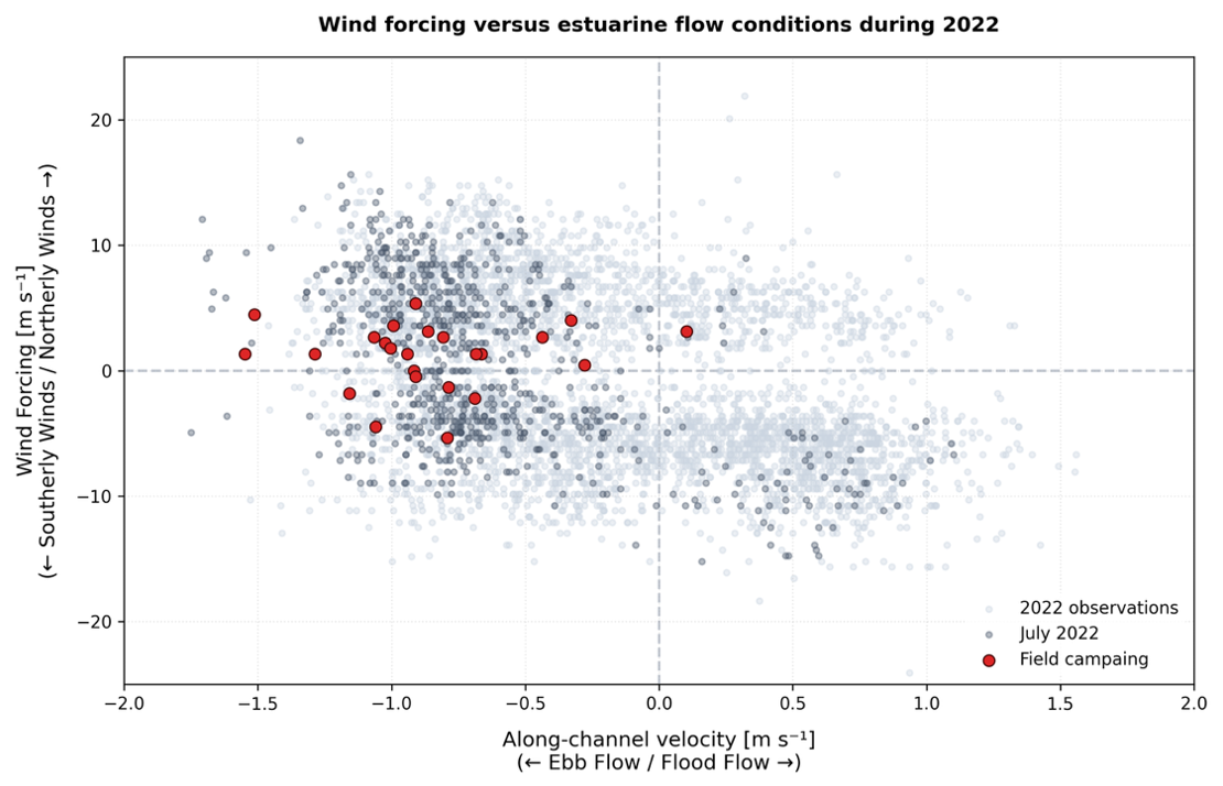
Figure 12 Wind–flow regime space for the Patos Lagoon during 2022. Gray symbols represent all observations available for 2022, dark gray symbols correspond to observations collected during July 2022, and red symbols indicate the conditions sampled during the field campaign. The x-axis shows the along-channel current velocity measured by the ADCP at approximately 3.5 m depth, used as a proxy for the estuarine exchange state (negative values indicate ebb flow and positive values indicate flood flow). The y-axis represents a signed wind-forcing proxy, with positive values corresponding to winds from the northern sector and negative values to winds from the southern sector. The clustering of the field observations within the July distribution indicates that the campaign sampled representative winter conditions within the dominant outflow regime of the Patos Lagoon.

5.2 Turbulence Variability Across the Estuary–Plume Continuum

The spatial distribution of the TKE dissipation rate (ϵ) along the drift segment highlights a clear maximum near the mouth and within the buoyant plume's surface layer. These high values align with the plume's “lift-off” zone (MacDonald and Geyer, 2004) and exhibit a decay proportional to the distance from the inlet (O'Donnell et al., 2008; McPherson et al., 2019). This maximum dissipation zone, associated with the plume's evolution over the quiescent coastal water, follows expected theoretical patterns for near-field river plumes (Horner-Devine et al., 2015).

Within the channel, the region of minimum ϵ between approximately km 4 and 7 coincides with an expansion of the cross-sectional area, suggesting the influence of the geometric widening. However, morphology alone is unlikely to explain the observed decrease in ϵ. The structure and magnitude of the along channel current does not change much in this sector, however the variability of ϵ may be related with the secondary circulation. Previous observations in the Rio Grande Channel demonstrated that secondary circulation could generate localized shear and enhance turbulent mixing through the interaction of baroclinic pressure gradients, channel curvature, and bathymetric forcing (Barros et al., 2025). Although the present survey captured a largely flushed and weakly stratified state within the inner channel, coherent lateral circulation patterns remain evident (Fig. 7b). Notably, the region of reduced ϵ between km 4 and 7 also corresponds to weaker cross-channel velocity gradients. This correspondence suggests that the observed decrease in turbulence may reflect not only the local channel expansion but also reduced shear production associated with secondary circulation.

As the flow approaches the final constriction near the mouth (dashed line, Fig. 13), the cross-sectional area decreases (approximately km 8–8.5), followed by an increase in ϵ values. However, the maximum dissipation rates (∼ 10⁻³ W kg⁻¹) occur immediately downstream of the inlet mouth, suggesting that, in addition to channel morphology, plume lift-off and the rapid transition from a laterally confined jet to an expanding buoyant plume contribute substantially to turbulence production. The combined action of these processes appears sufficient to overcome the stabilizing effect of the vertical density stratification, resulting in the intense mixing observed at the estuary–shelf interface.

Once the flow exits the jetties and enters the shelf, a reduction in ϵ is observed (Fig. 13). Although the buoyant plume remains vertically confined to the upper layer (Fig. 4a, c), the loss of lateral confinement permits rapid horizontal spreading. This transition from a topographically constrained jet to an expanding buoyant plume is accompanied by a marked decrease in ϵ, suggesting that the redistribution of momentum over a broader cross-sectional area contributes to the decay of turbulence and the transition away from the high-energy near-field regime.

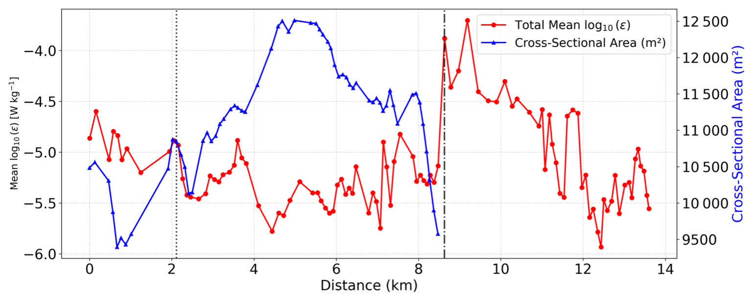
Figure 13 Longitudinal distribution of depth-average TKE dissipation rate (log₁₀ (ϵ), W kg⁻¹) and channel cross-sectional area (m²) as a function of distance. The red line (left y-axis) represents the average dissipation rate, while the blue line (right y-axis) indicates the cross-sectional area along the Drift segment. The dotted vertical line marks the initial channel widening, and the dash-dotted vertical line indicates the maximum constriction point (mouth) at the estuary–shelf interface.

The observations presented here represent the peak of a discharge event triggered by the relaxation of a meteorological sea-level set-up. As shown in Fig. 2d, the preceding landward wind stress promoted an inward water accumulation within the lagoon; once this forcing ceased, the resulting pressure gradient drove seaward flushing. This mechanism is a recurrent feature of the system's sub-tidal dynamics, where the passage of frontal systems every 5–7 d dictates the alternation between extreme outflow and salt-wedge intrusion (Möller et al., 2001; Fernandes et al., 2005). The comparison with Barros et al. (2025), conducted in the same area only 24 h later, highlights the remarkable temporal variability of the Patos Lagoon inlet. Whereas the previous study documented a salt-wedge configuration with a strong pycnocline that decoupled the surface flow from the bottom topography and suppressed turbulence, the present observations captured a fully flushed, inertia-dominated state in which peak discharge conditions exhibited a much stronger response to channel morphology.

These results suggest that, in microtidal environments, the temporal variability of mixing and turbulence can be governed primarily by synoptic forcing rather than by the predictable tidal cycle. The rapid shift observed here, from an inertia-dominated “flushed” state to a stratified “salt-wedge” intrusion state within only one day, highlights the importance of high-resolution spatial surveys to capture these transient regimes. In this context, the reduced tidal influence represents a key advantage, as it allows the isolation of wind-, discharge-, and morphology-driven processes that are often masked in strongly tidal systems. Therefore, these observations provide a useful framework for understanding the turbulent dynamics of estuarine–shelf systems, not only in microtidal environments but also in more complex settings where multiple forcings interact.

5.3 Hydraulic Adjustment Along the Estuary-Plume Transition

Considering the hydrodynamic transition along the Drift segment the evolution of hydraulic conditions along the estuary–plume transition was investigated. Based on the vertical density distribution and layer-averaged velocities (Fig. 14a–c), the internal Froude number (Fr) was calculated to characterize the flow's criticality (Fig. 14d). Such phenomena are common in estuarine plumes where the flow transitions from a supercritical (Fr > 1) to a subcritical (Fr_i < 1) regime. These transitions are often interpreted through idealized models of internal hydraulic jumps, though their application to natural, high-energy flows requires careful consideration of mixing and layer entrainment (Thorpe et al., 2017). The value of Fr is highly sensitive to the adopted parameters (interface depth, upper layer velocity and g^′).

In Fig. 14d, the blue line indicates the internal Froude number calculated using the parameters obtained for every vertical profile. The result is unexpected, to say the least, as it indicates the flow is supercritical over the entire section. Alternatively, the internal Froude number was calculated using a unique reference g^′, obtained based on the density difference between the channel's upper layer (∼ 1008 kg m⁻³) and the bottom coastal water (∼ 1022 kg m⁻³), following an approach suggested by Rock Geyer (personal communication, 2026), in similar fashion by MacDonald and Geyer (2005). This resulted in more expected values for the internal Froude number, and in reasonable agreement with MacDonald and Geyer (2005) values found in the uplift region of the Fraser River plume. A supercritical flow means the mean flow velocity is higher than the wave propagation velocity. As a consequence, the water surface becomes very agitated. The condition of a very agitated water surface was observed from the jetties' inlet outward for some distance. In the channel and offshore, away from the jetties' inlet, the sea surface was very calm, as the surveys were taken under breeze conditions.

The results using variable g^′ seem hard to interpret physically, which means the present case is out of the scope for its application. On the other hand, the use of a constant reference g^′ provides a nice fit to what is expected for the transition from channel flow to the early formation of the buoyant plume (Horner-Devine et al., 2015). From Figs. 7 and 8, it is possible to diagnose intense changes in plume velocity and thickness, and interfacial mixing, when the flow is supercritical. High surface velocities (∼ 2 m s⁻¹) resulted in elevated Fr_i values, as the flow's momentum far outweighed the stabilizing effect of buoyancy, even under sharp stratification. This supercriticality along the main axis is consistent with flow dynamics observed in energetic channel-to-plume transition zones, where high inertia and high-velocity discharge prevent immediate hydraulic adjustment to subcritical conditions (Dorrell et al., 2016).

Such momentum implies that the flow is too rapid for internal disturbances to propagate upstream (Nash and Moum, 2005). This observed vertical structure, which is characterized by a thin, high-velocity surface layer over a saltier ambient water mass, follows the conceptual model of strongly stratified river plumes documented in large-scale systems (Nash et al., 2009). While the supercritical flow blocks the upstream migration of internal waves, the intense velocity gradient it creates is precisely what triggers localized mixing. The strong shear at the plume's base may promote Kelvin-Helmholtz (KH) instabilities, which drive the recorded peaks in ϵ, a process consistent with observations in other highly stratified discharge regions (e.g., Spicer, 2022). The spatial correspondence between elevated ϵ (Fig. 13) and supercritical flow conditions (Fig. 14) indicates that substantial turbulent mixing can occur within the near-field plume before any hydraulic adjustment to subcritical conditions takes place.

The results suggest that hydraulic adjustment occurs ∼ 2 km offshore from the jetties' inlet, when Fr_i reduces to < 1. This is supported by the progressive decrease in velocity, the deepening of the surface layer interface (McPherson et al., 2020). The persistence of supercritical state over a few kilometres seaward of the mouth is a known feature of river plumes where the buoyant layer spreads laterally upon entering the ocean (Hetland, 2010; Horner-Devine et al., 2015). Under these conditions, the lateral straining of the shear layer acts as a persistent mechanism that promotes turbulent mixing. This process sustains elevated ϵ values across the region (Fig. 8) and delays the hydrodynamic transition to a subcritical state until substantial interfacial entrainment and lateral plume expansion are achieved (Geyer et al., 2017). The transition to the mid-field region, associated with subcritical conditions and reduced inertial dominance, is observed beyond km 11.

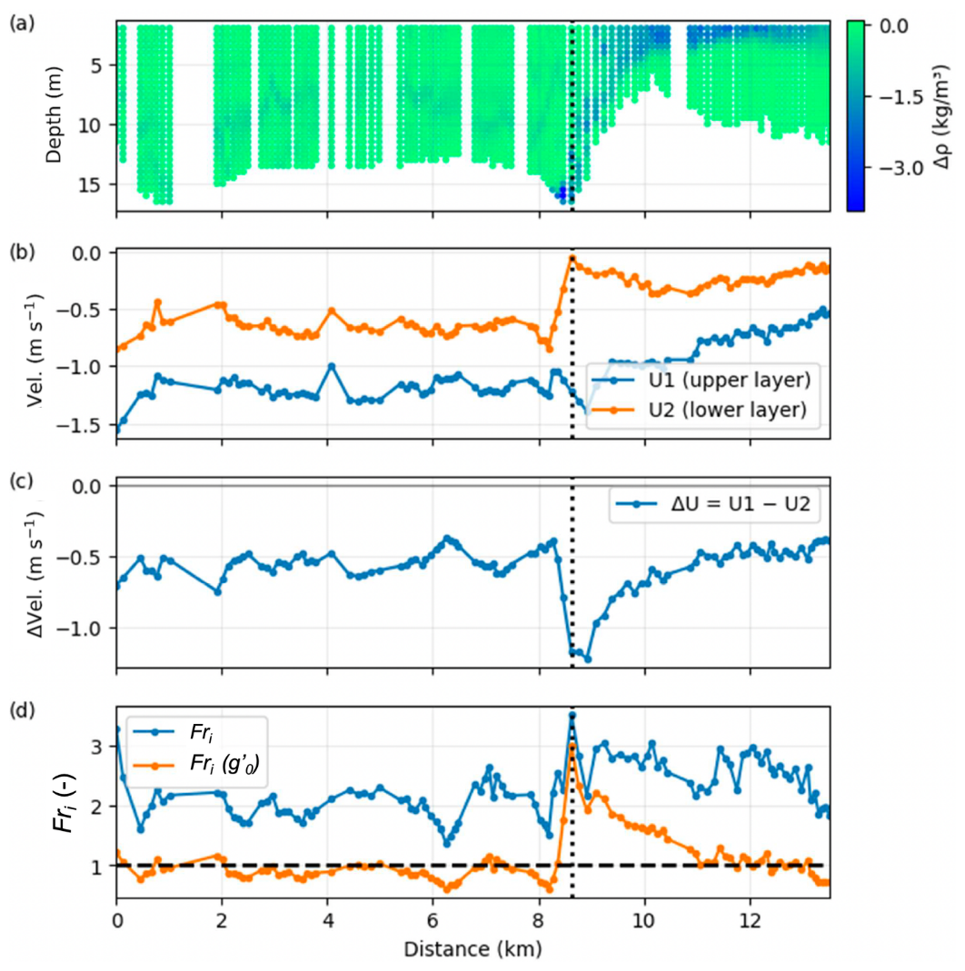
Figure 14 (a) Vertical density gradient (Δρ, kg m⁻³); (b) upper- and lower-layer horizontal velocities (U, m s⁻¹); (c) layer velocity difference (ΔU, m s⁻¹); and (d) the Internal Froude Number calculated based on g' calculated for every vertical profile (Fr_i), and alternatively using a reference $g_{\mathrm{0}}^{\prime }$. The dashed horizontal line in panel (d) indicates the critical threshold (Fr_i=1). The vertical dotted line marks the point of maximum constriction at the estuary–shelf interface.

5.4 Spatial Comparison and Estuarine Context

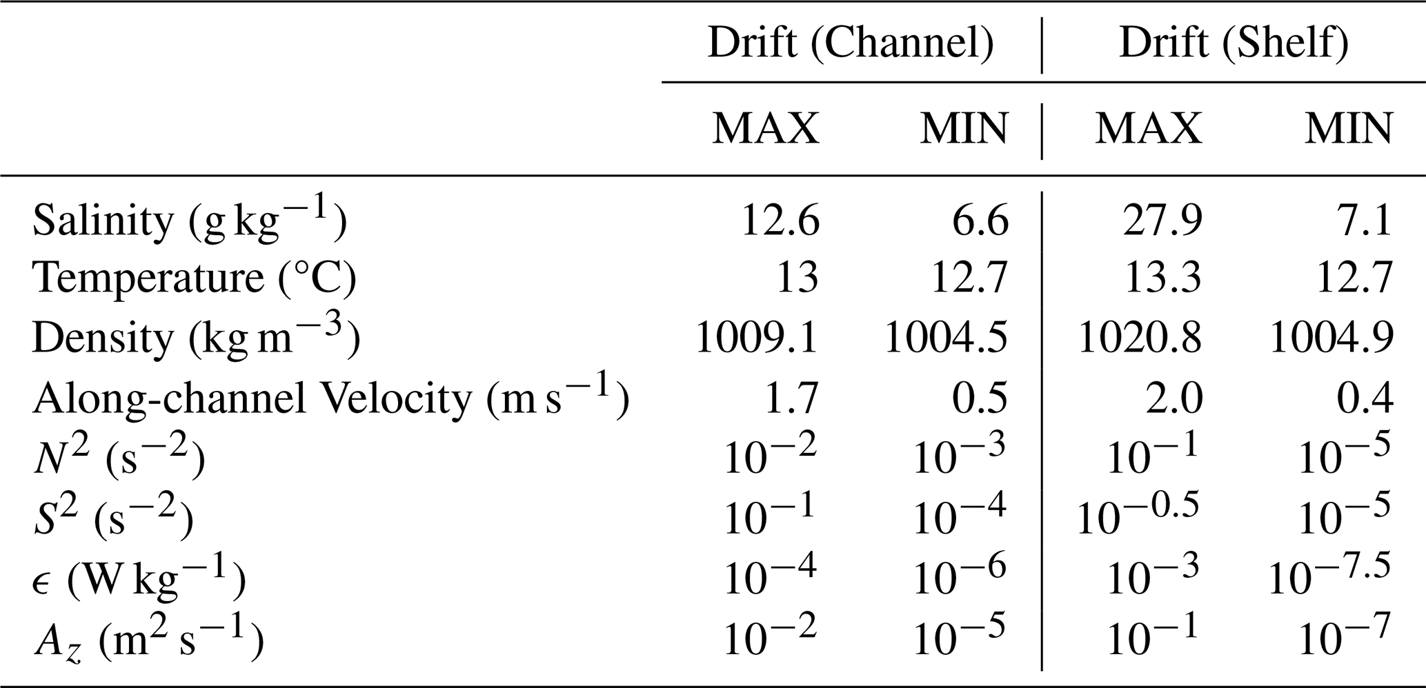
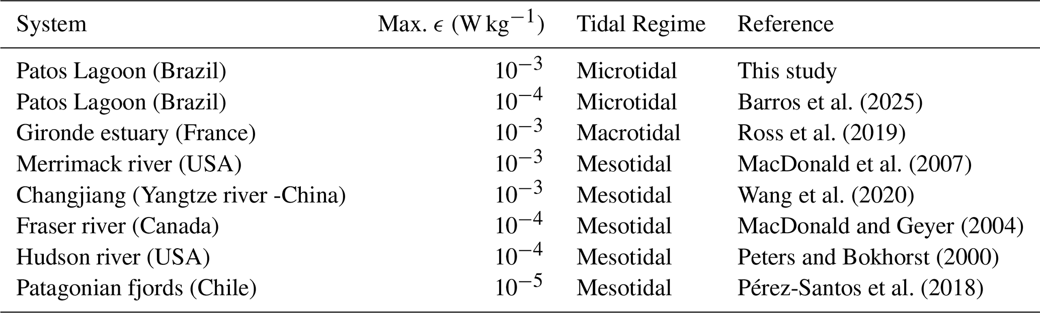
To evaluate the magnitude of the mixing processes observed, the maximum and minimum values of the primary hydrodynamic parameters were compared across the transition (Table 1) and contextualized with other estuarine systems globally (Table 2). The high-energy nature of the plume is initially evidenced by a peak in stratification (N² ∼ 10⁻¹ s⁻²) and vertical shear (S² ∼ 10^−0.5 s⁻²) that concentrate in the outer portion of the channel, marking the region of intense interfacial interaction (Fig. 9a, b). These conditions promote elevated TKE dissipation (ϵ), with peaks on the order of 10⁻³ W kg⁻¹ recorded immediately adjacent to the mouth (Fig. 8).

Table 1 Range of hydrodynamic and turbulent parameters observed inside the channel and on the adjacent shelf. Values represent the absolute minimum and maximum recorded during the drift survey.

As synthesized in Table 2, the maximum dissipation rates recorded at the Patos Lagoon mouth and its adjacent plume place this microtidal system among the most energetic estuarine environments documented in the literature. Furthermore, the extreme inertial dominance observed during this survey leads to dissipation rates that match or exceed those recorded in larger meso- and macrotidal systems, such as Gironde (Ross et al., 2019), Merrimack (MacDonald et al., 2007), Changjiang (Wang et al., 2020), Fraser (MacDonald and Geyer, 2004), and Hudson (Peters and Bokhorst, 2000) rivers. This energy level also significantly surpasses other topographically constrained environments in the Southern Hemisphere, including the Patagonian fjords, where tidal-driven turbulence at sills typically reaches values two orders of magnitude lower than those observed in the present study (Pérez-Santos et al., 2018).

Although direct comparisons should be interpreted cautiously due to differences in forcing conditions, sampling strategies, and methodologies among studies, the observed ϵ values place the Patos Lagoon Estuary within the upper range of turbulent conditions reported for energetic estuarine and plume environments. Rather than providing a strict ranking among systems, Table 2 is intended to provide a broader context for interpreting the magnitude of the observed mixing.

These results suggest that the primary distinction between microtidal and meso-macrotidal systems may lie in the forcing mechanisms responsible for generating turbulence rather than in the resulting mixing intensity. In the Patos Lagoon Estuary, turbulence levels comparable to those reported in energetic tidal systems developed under negligible tidal forcing, driven instead by the combined effects of sustained river discharge, persistent outflow, and strong topographic constriction at the inlet. These observations indicate that microtidal plumes can achieve similarly energetic states through fundamentally different forcing pathways.

Table 2 Representative examples of reported maximum TKE dissipation rates in estuarine environments.

Consistent with these high dissipation rates, the vertical eddy viscosity (A_z) reached maximum values of approximately 10⁻¹ m² s⁻¹ within the plume's interface (Table 1). This magnitude surpasses the maximum value of 10⁻² m² s⁻¹ previously observed in the Patos Lagoon inlet (Barros et al., 2025), reinforcing that under high outflow and specific morphological constraints, the Patos Lagoon inlet functions as a high-energy “nozzle” that maximizes turbulent transport to the inner shelf. Moreover, A_z spanned approximately six orders of magnitude across the surveyed domain over less than 14 km, revealing extreme spatial heterogeneity in mixing conditions. This variability highlights the difficulty of representing estuarine mixing using a single representative eddy-viscosity value and suggests that caution is warranted when adopting characteristic mixing parameters to describe estuary–plume systems, whether in classification frameworks or numerical modelling applications.

5.5 Turbulence and Mixing Processes

The buoyancy Reynolds number (Re_b) was applied to map the various stages of turbulence along the transect section (Fig. 10b). Dominant values of Re_b > 200 (blue points) are observed throughout most of the water column, indicating that vigorous, fully developed, and isotropic turbulence prevails in the system. In these regions, buoyancy forces are unable to inhibit the vertical transport of mass and momentum, a state that coincides with the high internal Froude number (Fr_i) values recorded (Fig. 14). This competition between shear and buoyancy was previously identified as a key driver of turbulence within the Patos Lagoon inlet (Barros et al., 2025), where Re_b often serves as a more sensitive indicator of mixing states than traditional stability metrics, as it directly scales the turbulence levels relative to the buoyancy-controlled Ozmidov scale (Stacey et al., 2012).

However, turbulence is locally suppressed within thin layers directly associated with the pycnocline interface (dashed line in Fig. 10b). In these specific pockets, particularly between km 4 and 8, Re_b < 15 occurs (red points), indicating a regime where stratification inhibits turbulent fluctuations and vertical mixing is restricted toward molecular levels (Shih et al., 2005). Surrounding these suppressed zones, a transitional regime (15 < Re_b < 200, yellow points) marks the areas where turbulence is active yet anisotropic. In this regime, despite the sharp stratification, the interfacial shear at the plume front promotes pycnocline erosion and subsequent saltwater entrainment. Such behaviour demonstrates that the presence of stratification does not necessarily imply the complete suppression of turbulent mixing, even under established stratification (Huguenard et al., 2015).

This spatial distribution suggests that while the plume's massive inertia maintains a state of generalized high-energy mixing, the density interface still acts as a localized, albeit intermittent, barrier to vertical transport. In this context, metrics based on the Richardson number (Ri) provide a consistent view of the potential for stratification-driven stability, particularly near the mouth and along the offshore interface, where it indicates a robust buoyancy barrier (Fig. 9c).

Nevertheless, the presence of these stable Ri layers does not necessarily imply the absence of mixing in such high-energy systems. While Ri ≈ 0.25 is commonly interpreted as a classical threshold for the onset of shear instability, recent studies have emphasized that this criterion is strictly applicable only when Richardson number is evaluated over sufficiently small vertical scales (MacDonald and Goodman, 2026). In field observations, Richardson number estimates are often evaluated over observational scales that are larger than those associated with the onset of individual shear instabilities. Under these conditions, turbulence may persist for Ri values substantially greater than 0.25 because unresolved sublayers can locally satisfy instability criteria and sustain turbulent production. Therefore, the classical threshold alone is not sufficient to fully describe mixing in natural environments, as turbulence may be sustained for Ri values approaching unity under energetic forcing conditions (Simpson and Sharples, 2012). This perspective is particularly relevant in the present study, where elevated ϵ and Re_b values frequently coexist with R_i values above the classical instability threshold. As observed between km 9 and 10, even where Ri suggests stability, the buoyancy Reynolds number (Re_b) and elevated ϵ confirm that turbulence remains vigorous enough to dynamically erode the interface. In estuarine environments, this corresponds to an intermediate regime (0.25 < Ri < 1), where mixing is not suppressed but instead modulated by the interplay of shear, straining, and advection (Giddings et al., 2011).

These results suggest that the classical Ri threshold alone may not fully capture the complexity of mixing dynamics in this system. Such limitations of the gradient Richardson number as a universal mixing proxy have been recently documented in other diverse high-energy, wind-dominated systems (Arevalo et al., 2022; Álvarez‐Silva et al., 2026), where vigorous mixing and asymmetric hydrodynamic structures persist even under seemingly stabilizing density gradients. While the transitional criteria Re_b=15 and 200 inherently involve statistical uncertainty and scale dependencies, the buoyancy Reynolds number (Re_b) provides a more robust description of turbulent efficiency in this energetically active plume, capturing the full spectrum of mixing states that traditional stability thresholds may overlook.

6 Conclusions

This study provides a detailed characterization of the estuary-shelf transition of a buoyant plume during a period of high discharge, revealing how channel morphology, secondary circulation, and plume adjustment processes interact under inertial dominance to control turbulent mixing across the estuary–plume continuum. The Patos Lagoon inlet, despite its microtidal regime, represents a high-energy benchmark for global estuary-shelf transitions, where the terminal jetty constriction acts as a morphological “nozzle” that contributes to the development of an extremely energetic state. These high dissipation levels, reaching 10⁻³ W kg⁻¹ near the mouth, are comparable to those found in major meso- and macrotidal systems and are driven by surface velocities of ∼ 2 m s⁻¹, where inertial momentum far outweighs the stabilizing effects of buoyancy.

The along-channel evolution of turbulent kinetic energy (TKE) dissipation reflects the combined influence of channel morphology, secondary circulation, and plume adjustment processes. Dissipation rates (ϵ) are significantly reduced within the inner estuary where the cross-sectional area widens, coinciding with weaker cross-channel velocity gradients, while maximum values occur near the jetty-confined mouth. Following this peak, ϵ values decrease progressively as the flow spreads offshore and the plume expands laterally.

Diagnosed using the internal Froude number, the observations indicated a transition from subcritical flow in the channel to supercritical flow in the buoyant plume liftoff zone, followed by a return to subcritical flow offshore. However, this result was obtained using a single reference value of g^′ for the entire dataset. When local values of g^′ were used for each vertical profile, the entire section was classified as supercritical, which appears inconsistent with the observed sea state and suggests that the use of local g^′ may not be appropriate for diagnosing the flow regime in this case.

Within this high-energy, supercritical regime, the interplay between buoyancy suppression and shear production is effectively captured by the buoyancy Reynolds number (Re_b). This parameter accurately identifies the turbulence suppression observed near km 6, consistent with the localized minima in TKE dissipation. Furthermore, at the plume's frontal interface (∼ km 9), Re_b provides a clearer explanation of the mixing state than the Richardson number; while Ri identifies the structural potential for stability along the interface, Re_b indicates that turbulence remains sufficiently energetic to overcome buoyancy constraints (Re_b > 200). This contrast highlights the limitation of relying solely on stability-based metrics to describe mixing in such energetic environments.

The findings of this study highlight the combined influence of inlet morphology, secondary circulation, and plume adjustment processes in modulating the hydrodynamic structure and mixing regimes of high-energy river plumes, suggesting that similar interactions may occur in other wind-dominated, microtidal estuaries. More broadly, the results suggest that the primary distinction between microtidal and meso-/macrotidal plume systems may lie in the forcing mechanisms responsible for generating turbulence rather than in the resulting mixing intensity. In the Patos Lagoon estuary, turbulence levels comparable to those reported in energetic tidal systems developed under negligible tidal forcing, driven instead by sustained river discharge, persistent outflow, and strong topographic constriction at the inlet.

While these results provide a detailed characterization of the estuary–plume continuum under high-discharge conditions, several key questions remain unresolved. Explicitly closing the momentum budget throughout the estuary–plume transition, identifying the location and mechanisms of hydraulic adjustment in the mid- to far-field plume, and quantifying the role of lateral plume spreading in controlling entrainment and mixing represent important directions for future research. Addressing these processes through targeted field observations will be essential to advance our understanding of microtidal plume dynamics and their broader influence on estuary–shelf exchange.