Storm-modulated submesoscale dynamics over sloping topography in a wind-driven, non-tidal basin

While ocean surface submesoscales have been extensively studied, their counterparts in the bottom boundary layer (BBL) remain little explored. These subsurface features, however, appear to play a key role in (i) boundary-interior exchange, (ii) forward energy cascade, and (iii) turbulent boundary mixing, which is an important driver of the overturning circulation. Since interior submesoscales typically arise through flow-topography interactions, recent studies have focused on their genesis in the open ocean, particularly in regions where strong, relatively steady currents flow over steep slopes. Here, we use the Baltic Sea as a natural laboratory to show that submesoscales are widespread even in semi-enclosed basins, far from major current systems, in regions where tides are virtually absent, and ephemeral wind-driven currents typically dominate. Using high-resolution numerical simulations, we demonstrate that surface and subsurface submesoscales can coexist, with the latter being especially prominent near the lateral boundaries. Strong ageostrophic features emanate from the boundaries and are accompanied by potential vorticity anomalies, indicating regions prone to instabilities. Oppositely signed vorticity is typically found at either side of the basin, intensifying locally during strong winds. By analyzing a series of sequential storm events with opposing winds, we show that variability in wind direction is important in determining the submesoscale generation sites and mixing hotspots. Wind reversals reverse the regional circulation and lead to alternating vorticity signals within the BBL, suggesting that the submesoscale generation sites and mixing hotspots exhibit transient behavior. Our findings highlight the previously unrecognized, broader significance of storm-modulated submesoscales in wind-driven marine and limnic systems, extending their relevance beyond the Baltic Sea.

1 Introduction

Submesoscales are ephemeral oceanic features in the form of vortices, density fronts, and filaments, with horizontal scales ranging from 0.1 to 10 km and lifetimes of hours to days, concentrating mainly in the weakly stratified surface layer and the bottom boundary layer (BBL). Unlike mesoscale dynamics, where vertical stratification dominates and planetary rotation firmly constrains the flow, submesoscale structures are still influenced but only weakly constrained by the Earth's rotation (Capet et al., 2008; McWilliams, 2016). Dynamically, they can thus be defined as flows for which the Rossby and balanced Richardson numbers,

$$\begin{array}{}\text{(1)}& \mathit{Ro}={\displaystyle \frac{\mathit{\zeta }}{f}},{\mathit{Ri}}_b={\displaystyle \frac{f^{\mathrm{2}}{N}^{\mathrm{2}}}{\mathrm{|}{\mathrm{\nabla }}_{\mathrm{h}}b{\mathrm{|}}^{\mathrm{2}}}},\end{array}$$

are both 𝒪(1). Here, f denotes the planetary vorticity, $\mathit{\zeta }=v_x-u_y$ the vertical component of the relative vorticity, $N^{\mathrm{2}}=\partial b/\partial z$ the square of the buoyancy frequency, where $b=-g(\mathit{\rho }-{\mathit{\rho }}_{\mathrm{0}})/{\mathit{\rho }}_{\mathrm{0}}$ is the buoyancy based on the (potential) density ρ (g is the gravitational acceleration, and ρ₀ a constant reference density), and ∇_h denotes the horizontal nabla operator.

While surface submesoscales have been extensively studied and different mechanisms have been proposed for their emergence, their counterparts in the BBL remain little explored. However, recent modeling efforts (Molemaker et al., 2015; Gula et al., 2015), supported by scarce observational data (Bosse et al., 2017; Garabato et al., 2019; Gula et al., 2019), suggest that submesoscales are abundant in the oceanic interior, challenging the traditional view of a quiescent, stratified interior in quasigeostrophic equilibrium (Siegelman, 2020). These ageostrophic features, which primarily emerge from the interaction of geostrophic flows with steep topographic slopes (as explained below), are dynamically important, as they provide a direct pathway for the forward cascade of mesoscale energy toward dissipation scales (Gula et al., 2022).

Specifically, Molemaker et al. (2015) showed that when an interior current flows above a sloping bottom, the drag against the slope will create not only vertical but also significant horizontal velocity shear, i.e., vertical vorticity. Currents with large vertical vorticity may become unstable, separate from the slope, especially at locations of strong topographic curvature, and form turbulent topographic wakes. In the separated wake, submesoscale instabilities typically emerge, resulting in enhanced energy dissipation and the formation of submesoscale coherent vortices (Chor and Wenegrat, 2025). This process has been shown, for example, in the context of the California Undercurrent (Molemaker et al., 2015; Dewar et al., 2015), the Gulf Stream (Gula et al., 2015, 2019), and the Kuroshio–Oyashio Extension (Zhu et al., 2024). The resulting submesoscale coherent vortices are usually long-lived, which enables them to transport their anomalous physical and biogeochemical properties over long distances away from the generation sites (D'Asaro, 1988; Frenger et al., 2018; McCoy et al., 2020). More recently, observations from a deep western boundary current in the Southern Ocean have further highlighted the role of submesoscale instabilities in driving boundary–interior exchange and turbulent boundary mixing (Garabato et al., 2019).

The aforementioned studies have explored the emergence of interior submesoscales by focusing particularly on the vicinity of strong current systems (Molemaker et al., 2015; Dewar et al., 2015; Gula et al., 2016), coastal jets (Capó et al., 2023) and dense water outflows (Vic et al., 2015). Here the focus is on wind-driven, non-tidal marine and inland water systems that do not include western boundary currents or other large-scale current systems. Examples include semi-enclosed marine systems like the Baltic Sea, the Black Sea, and large limnic systems like the Great Lakes in North America and the Caspian Sea. Our goal is to investigate how wind events influence the deep-water submesoscale dynamics in such wind-driven systems, complementing the study of Chrysagi et al. (2021), which focused on the effects of storms on surface-layer submesoscale dynamics. We therefore use a realistic high-resolution numerical simulation to study the emergence of these features during sequential storm events.

Our study area is the Baltic Sea, a shallow and strongly stratified brackish marine system connected to the North Sea through the Danish Straits (Fig. 1a). Persistent lateral density gradients and rich submesoscale activity dominate in the surface mixed layer (Väli et al., 2017; Zhurbas et al., 2022; Chrysagi et al., 2021, 2022; Lips et al., 2026), whereas mesoscale eddies are found at various depths, concentrating in the pycnocline (Reissmann et al., 2009; Vortmeyer-Kley et al., 2019). Temporal variability of currents is high in response to variable atmospheric forcing (Liblik et al., 2022). Wind forcing plays an important role in driving the circulation, influencing not only the surface but also the deeper layers of the basin (Krauss and Brügge, 1991; Lehmann and Myrberg, 2008; Zhurbas and Väli, 2022).

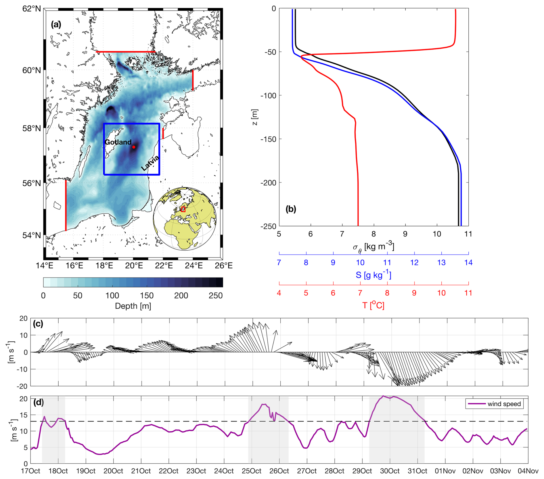
Figure 1 (a) Model domain (central Baltic Sea, known as Baltic Proper) and bathymetry. Red lines indicate the open boundaries of the model, the blue box shows the study area (Eastern Gotland Basin), and the red dot marks the position of the profiles shown in panel (b). (b) Vertical profiles of density, salinity, and temperature at the deepest point of the Eastern Gotland Basin (Gotland Deep) on 29 October 21:00 UTC. (c) Basin-averaged wind speed and direction throughout the study period (October/November 2017). (d) Basin-averaged wind speed magnitude, with the dashed horizontal line indicating the 13 m s⁻¹ threshold used to define storm events. The light gray shaded areas indicate the approximate duration of the three successive storm events.

The response of a stratified, elongated basin to constant alongshore wind forcing was described for the Baltic Sea by Krauss and Brügge (1991) and by Lehmann and Myrberg (2008). It involves cross-shore Ekman transport in the surface layer, leading to a sea-level rise along one coast and a corresponding sea-level fall along the opposite coast. This induces downwelling and upwelling, respectively, and associated baroclinic responses at both coasts. Consequently, coastal jets develop along both coasts in the direction of the wind, accompanied by a compensating return flow in the basin interior. Such bottom countercurrents, directed opposite to the wind, can arise as a response to the developed coastal jets (Krauss and Brügge, 1991) or, in some cases, prevail as a result of open-sea wind-driven Ekman transport (Zhurbas and Väli, 2022). Coastal upwelling/downwelling events and the formation of wind-driven boundary currents are commonly observed and can occur concurrently at the basin's eastern and western sides (Lehmann and Myrberg, 2008; Lips et al., 2026). The circulation therefore rapidly reacts to the wind forcing, with wind reversals followed by current reversals in the deeper layers occurring frequently in the basin (Liblik et al., 2022; Zhurbas and Väli, 2022). We thus hypothesize that such wind-driven changes in the direction and structure of the interior circulation can, in turn, influence the development of submesoscale features.

We focus particularly on the Eastern Gotland Basin (blue box in Fig. 1a), which is characterized by a permanent halocline, typically centered at around 70 m depth (Fig. 1b). The strong halocline acts as a natural lid, isolating the oxygen-rich surface water from the typically anoxic deeper layers of what is one of the globally largest anoxic marine systems. As tides are virtually absent and diapycnal mixing is weak, the primary process ventilating the oxygen-depleted bottom waters is short-lived intrusion events (Major Baltic Inflows; Reissmann et al., 2009; Mohrholz, 2018; Löptien et al., 2025), which import oxygenated waters from the North Sea. A tracer release experiment and turbulence microstructure observations (Holtermann et al., 2012; Holtermann and Umlauf, 2012) have shown that basin-scale vertical deep-water mixing in the central Baltic Sea is largely driven by boundary processes, fueled by wind-driven topographic waves and, to a smaller extent, by near-inertial waves generated by transient wind forcing (Holtermann and Umlauf, 2012; Holtermann et al., 2012, 2014). At present, however, the processes governing the exchange between mixed boundary-layer waters and the weakly turbulent interior of the Baltic Sea remain poorly understood, and the potential role of subsurface submesoscale motions has not yet been investigated in detail.

Here, the Baltic Sea is used primarily as a natural laboratory to enable the investigation of interior submesoscale phenomena in a semi-enclosed, wind-driven basin, placed in the context of the more familiar open-ocean submesoscales that arise near stationary, large-scale boundary currents. Our goal is to show that in such basins, intense and variable winds can strongly influence submesoscale motions – a hypothesis that is likely to be broadly applicable to other wind-driven marine basins and large lakes. The manuscript is organized as follows. Section 2 introduces the model setup, the atmospheric conditions, and the analysis methods. In Sect. 3, we explore the co-existence of surface and subsurface submesoscales, immediately following a severe storm episode. Section 4 highlights the main characteristics of the wind-driven submesoscales emerging in the stratified interior, below the pycnocline. Section 5 investigates the formation of these features during sequential wind events by exploring the effects of wind magnitude and direction. In Sect. 6, we examine the different instability types emerging in the BBL during storms. The main findings of our study are summarized in Sect. 7.

2 Model description and methods

2.1 Numerical model

To investigate the submesoscale motions in the oceanic interior and their response to storms, we conducted realistic high-resolution simulations using the General Estuarine Transport Model (GETM; Burchard and Bolding, 2002). Since the same simulation setup was used in Chrysagi et al. (2021) to study the submesoscale dynamics in the surface layer, only the most relevant model features are presented here. For further details on the numerical model, the simulation setup, and the model validation, the reader is thus referred to the aforementioned study.

The model domain covers the entire central Baltic Sea (known as Baltic Proper), spanning from 54.2 to 60.6° N, and from 15.5 to 24.0° E (Fig. 1a). The horizontal grid size varies between 500 and 600 m, which, as shown in Chrysagi et al. (2021), is sufficient to allow for the emergence of submesoscales. In the vertical, 100 adaptive, topography-following layers are applied. The use of such an adaptive numerical grid that follows the evolution of stratification and shear (Burchard and Beckers, 2004; Hofmeister et al., 2010), reduces numerical mixing and pressure gradient errors (Gräwe et al., 2015), and yields a high-resolution representation of the turbulent BBL (Holtermann et al., 2014). The lateral boundary conditions (model boundaries marked in red in Fig. 1a) are extracted from the 1 nautical mile (NM) Baltic Sea model of Gräwe et al. (2019). Initial conditions were obtained by merging existing GETM simulations from Holtermann et al. (2014) and observed Conductivity-Temperature-Depth (CTD) profiles of the central Baltic Sea, extracted from the HELCOM database (http://www.helcom.fi, last access: 1 October 2026). As the spatial coverage of the measurements is rather low, model data were nudged towards the CTD profiles by applying a distance-weighted algorithm, based on a Gaussian function with a standard deviation of 10 NM. Thus, the initial data correspond to the CTD data directly at the position of the profiles, whereas at 10 NM distance, 61 % of initial profiles are taken from the CTD casts and the rest from the model output. The simulation is then run freely without any nudging from 1 February 2016 to 31 December 2017. The atmospheric forcing is taken from the German Weather Service (DWD) operational model with spatial and temporal resolutions of 7 km and 3 h, respectively.

The horizontal diffusivities are parameterized according to Smagorinsky (1963) using a Smagorinsky constant of 0.6 and a turbulent Prandtl number of 2.0 for tracers. The vertical mixing is parameterized through a two-equation turbulence model with one prognostic equation for the turbulent kinetic energy, k, and one for its dissipation rate, ε (k-ε model; Umlauf and Burchard, 2005). An algebraic second-moment turbulence closure model is applied to calculate the vertical turbulent viscosity, A_ν, and the vertical turbulent diffusivity, K_ρ (Canuto et al., 2001; Umlauf and Burchard, 2005). To mimic the unresolved mixing in the interior region, induced e.g., by internal wave breaking, we prescribe a background turbulent kinetic energy level of k_min = 10⁻⁷ m² s⁻², and limit the turbulent length scale by the Ozmidov scale (Galperin et al., 1988; Umlauf and Burchard, 2005). Close to the bottom, we make the standard assumption that the velocity follows the logarithmic wall profile for a hydrodynamically rough bottom. This implies a quadratic friction law based on a constant bottom roughness of z₀ = 0.002 m, as described in detail in Klingbeil et al. (2018).

The model has been validated using satellite data from BSH (German Federal Maritime and Hydrographic Agency), several vertical temperature and salinity profiles from long-term moorings (HELCOM standard monitoring program), along with in-situ, high-resolution CTD data collected using a free-falling turbulence microstructure profiler (for details see Sect. 3 in Chrysagi et al., 2021). Our analysis focuses on the Eastern Gotland Basin (blue box in Fig. 1a), the largest basin of the Baltic Proper with a maximum depth of approximately 250 m. The study period is restricted from 17 October to 4 November 2017, aiming to simulate a field campaign that was carried out in the Eastern Gotland Basin with a focus on submesoscale structures. Throughout the observational campaign, stormy weather conditions dominated (Sect. 2.2). While Chrysagi et al. (2021) focused on the role of storm events on the surface submesoscale motions, here we explore whether storms can also trigger such motions in the stratified interior, below the main pycnocline. To illustrate the genesis of submesoscales, a passive tracer is released 16 d prior to the study period (1 October) into the BBL at 80 m depth to highlight the topographically generated motions and the boundary-interior exchanges (see Sect. 4).

2.2 Atmospheric conditions

During the period of interest, three consecutive storms (i.e., wind speed exceeding 13 m s⁻¹; see Fig. 1d) occurred in the Eastern Gotland Basin, with the winds blowing from different directions (Fig. 1c). The first storm passed over the area around 18 October 2017 with south-southwesterly winds, the second around 25 October with pronounced southerly winds, and the third peaking on 30 October with winds from a northerly direction. A maximum value of 20 m s⁻¹ was observed during the last storm, whereas the lowest wind speeds occurred on 19 October, with values as small as ∼ 2 m s⁻¹. As discussed in the following sections, the highly variable winds strongly influenced both the magnitude and direction of the currents, and thereby the locations of submesoscale generation and mixing hotspots. While the first two storms created an extended upwelling zone near the island of Gotland (location is shown in Fig. 1a), the last storm with opposing winds favored coastal upwelling along the Latvian coast (Fig. 1a). Such wind events, followed by coastal upwelling/downwelling and development of along-slope boundary currents, are quite common in the Baltic Sea (Lehmann and Myrberg, 2008) and, therefore, the dynamical processes outlined in the following sections are expected to occur frequently.

2.3 Analysis methods

The genesis of submesoscales in the subsurface layers of the ocean, below the surface mixed layer, has been primarily linked to the interaction of strong geostrophic currents with steep topographic slopes. Molemaker et al. (2015) showed that vertical relative vorticity,

$$\begin{array}{}\text{(2)}& \mathit{\zeta }=\widehat{\mathit{z}}\cdot \mathrm{\nabla }\times \mathit{u}={\partial }_{x}v-{\partial }_{y}u,\end{array}$$

where $\widehat{\mathit{z}}$ is the upward unit vector, can be generated through lateral drag on an along-slope current. The vorticity ζ will be positive (cyclonic) for currents flowing with the topographic slope on their left, whereas negative (anticyclonic) ζ is expected for flows moving in the direction of a Kelvin wave (Northern Hemisphere). The current direction is therefore crucial for submesoscale dynamics. As discussed below, in wind-driven systems, ζ and therefore Ro (see Eq. 1) may show alternating patterns induced by changes in the wind direction, a behavior that is not typically expected in large-scale current systems where the flow direction is generally unchanged (especially in the interior). Intensification of winds, on the other hand, may cause enhanced velocity shear, resulting in strong Ro and ultimately triggering various types of instabilities.

To distinguish between the different instability types, we will use the Ertel potential vorticity (EPV):

$$\begin{array}{}\text{(3)}& q=(f\widehat{\mathit{z}}+\mathrm{\nabla }\times \mathit{u})\cdot \mathrm{\nabla }b.\end{array}$$

Following the analysis presented in Thomas et al. (2013), (Eq. 3) can be decomposed into two terms:

$$\begin{array}{}\text{(4)}& q=q_{\mathit{\zeta }}+q_{\text{bc}}.\end{array}$$

The first term is associated with the absolute vertical vorticity, ${\mathit{\zeta }}_{\text{abs}}=f+\mathit{\zeta }$, and stratification, $N^{\mathrm{2}}=\partial b/\partial z$, and is given by:

$$\begin{array}{}\text{(5)}& q_{\mathit{\zeta }}={\mathit{\zeta }}_{\text{abs}}{N}^{\mathrm{2}}.\end{array}$$

The second term is related to the baroclinicity of the flow, and is defined as:

$$\begin{array}{}\text{(6)}& q_{\text{bc}}=\left({\displaystyle \frac{\partial u}{\partial z}}-{\displaystyle \frac{\partial w}{\partial x}}\right){\displaystyle \frac{\partial b}{\partial y}}+\left({\displaystyle \frac{\partial w}{\partial y}}-{\displaystyle \frac{\partial v}{\partial z}}\right){\displaystyle \frac{\partial b}{\partial x}}.\end{array}$$

Different overturning instabilities (Garabato et al., 2019) can occur if the EPV and Coriolis parameter have the opposite sign, i.e., fq<0 (Hoskins, 1974). For N²<0, gravitational instability may occur. Under stable stratification (N²>0), centrifugal or inertial instability arises if fq_ζ<0. Symmetric instability (SI) occurs for N²>0 if fq_ζ>0 and |fq_bc|>fq_ζ (Thomas et al., 2013). Note that our horizontal grid resolution is likely not sufficient to fully resolve such small-scale instabilities. However, using the same configuration, Chrysagi et al. (2021) demonstrated that in regions where the criteria for SI are satisfied, the modeled energy dissipation rates are in good agreement with the theoretical estimates of Thomas and Taylor (2010), suggesting that the bulk energetics of SI are represented. As shown below, the instability conditions are satisfied near the lateral boundaries, where we identify regions with fq<0. The resulting vorticity anomalies are subsequently advected into the stratified interior in the form of eddies, fronts and filaments.

3 Surface-layer and deep-water submesoscale phenomena

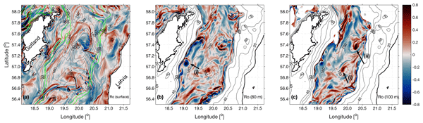
At the peak of the last storm event (31 October 2017), Rossby number maps reveal a wealth of small-scale structures at all depth levels (Fig. 2). Features with enhanced Ro appear not only in the surface layer (Fig. 2a) but also in the deeper parts of the water column (Fig. 2b and c), especially close to the sloping boundaries. Inside these features, we find widespread regions with Ro=𝒪(1), suggesting that submesoscale processes form an important component of the deep-water dynamics also in this shallow wind-driven marine system.

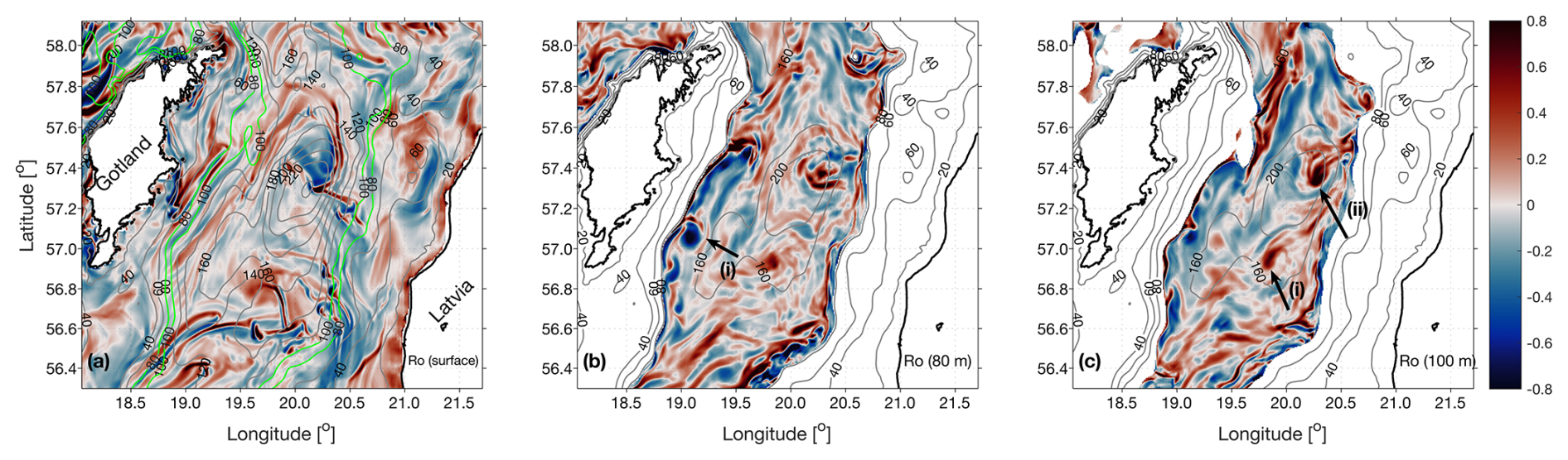
Figure 2 Surface-layer and deep-water submesoscale features. Rossby number (Ro) snapshots (a) in the surface layer (2 m depth), (b) below the main pycnocline (80 m), and (c) in the interior (100 m) of the Eastern Gotland Basin for 31 October 2017 09:00 UTC (storm conditions). The gray contours in all panels show the topography, whereas the green lines in (a) delineate the 80 and 100 m bathymetry contours. Black arrows indicate eddy-like features.

Focusing on the surface layer, numerous fronts and filaments can be identified from the spatial distribution of the near-surface Rossby number (Fig. 2a). Chrysagi et al. (2021) showed that these features are characterized by shallow mixed layers even during periods of strong wind forcing, due to submesoscale restratification. Their emergence was shown to be linked to a large-scale persistent frontal structure which, during autumn, occupies the entire eastern part of the basin. Typically, the surface submesoscale phenomena stay confined to the weakly stratified surface mixed layer, and therefore have no signature in the deeper layers (McWilliams, 2016).

Figure 2b, c show that submesoscale features with Ro=𝒪(1) are ubiquitous also in the stratified interior region below the permanent pycnocline. These features are not spatially correlated to their counterparts in the surface layer, suggesting an independent generation mechanism. Significantly higher values of Ro close to the lateral boundaries, with some ageostrophic patterns extending further offshore, away from the sloping bottom, provide an initial indication of the relevance of submesoscale generation sites near the boundaries. A prominent example is the anticyclonic vortex with a strongly negative vorticity core that develops during the northerly storm (marked by the black arrow in Fig. 2b). Two eddy-like features with positive Ro=𝒪(1) are also visible, particularly at 100 m depth (black arrows in Fig. 2c). These features were formed during the first wind episode (see also Fig. 3 below) and have a boundary origin, potentially arising from flow-topography interactions, as noted in previous studies (Molemaker et al., 2015; Gula et al., 2015; McWilliams, 2016; Contreras et al., 2019).

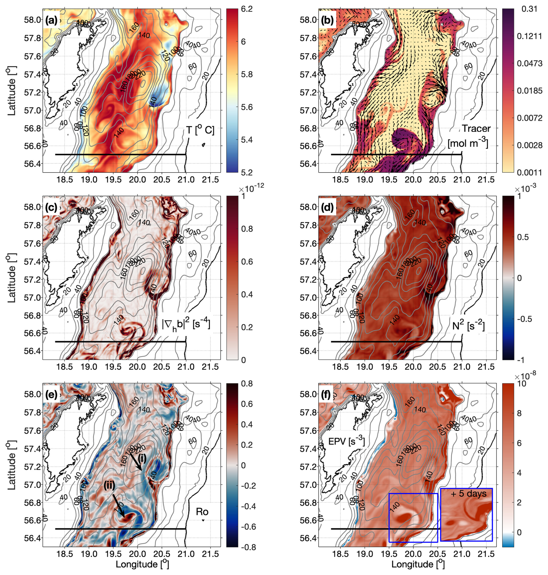
Figure 3 Spatial distribution of various metrics indicative of the submesoscale nature of the flow in the interior region at 80 m depth: (a) temperature, (b) tracer distribution and circulation (arrows), (c) frontal sharpness, defined as |∇_hb|², (d) buoyancy frequency squared, and (e) Rossby number. Black arrows show eddy-like structures. The eddy-like feature, marked as (ii), is also visible in Fig. 2c, marked as (i). (f) Ertel potential vorticity (EPV), with negative values indicating the instability regions. Gray lines denote isobaths, whereas the black line indicates the location of the transect that is further analyzed in Fig. 4. All patterns are instantaneous fields on 22 October 03:00 UTC, after the first wind event. The embedded panel in (f) shows the EPV 5 d later on 27 October.

Overall, small-scale structures with enhanced Ro=𝒪(1) are ubiquitous at the peak of the storm, both at the surface and in the deeper layers. However, the surface and the interior regions exhibit distinct and phenomenologically disconnected patterns, especially near the lateral margins. This suggests that surface and subsurface submesoscale motions are able to coexist while remaining dynamically isolated from each other. This contrasts with previous studies (e.g., Gula et al., 2016; Capó et al., 2023) showing that submesoscale motions observed in the surface layer were formed above sloping topography, and thus had an interior origin. Building on existing understanding, our investigations will therefore concentrate on the emergence of submesoscales in the deeper layers, below the main pycnocline, focusing particularly on the role of wind events in modulating these phenomena in a predominantly wind-driven, non-tidal system.

4 Wind-induced submesoscale phenomena in the stratified interior

To explore the spatial distribution of the flow after the first wind event, horizontal slices of various dynamical quantities at 80 m depth are shown in Fig. 3, where the signatures of fronts, filaments, and spiral-like features are clearly visible. Close to the lateral margins, particularly large horizontal buoyancy gradients (Fig. 3c), often combined with Ro=𝒪(1) (Fig. 3e), indicate submesoscale dynamics. The pronounced |∇_hb|² patterns also have a signature in the temperature field, where boluses of colder water can be spotted throughout the basin (Fig. 3a). Figure 3b shows the spatial distribution of the passive tracer, released at 80 m depth exclusively within the BBL 16 d prior to the study period (Sect. 2.1). The tracer shows distinct features that correlate strongly with those observed in the buoyancy gradients. These features are ageostrophic, as evident from the large Ro values (Fig. 3e), and seemingly control the lateral dispersion of the tracer by initially trapping it and then transporting it away from the boundary, into the stratified interior.

A spatial discrepancy between the western and eastern margins of the basin is visible from Fig. 3e and f. In the west, thin stripes of negative vorticity appear that tend to follow isobaths, whereas in the east, positive vorticity signals dominate. The negative relative vorticity (or Ro<0, Fig. 3e) along the slope east of the island of Gotland is generated by lateral topographic drag on the southward flow (black arrows in Fig. 3b). Similarly, regions with large Ro>0 develop along the Latvian coastline as the current flows with the coast to its left, such that topographic drag now generates cyclonic shear. This is consistent with numerous studies demonstrating that flow-topography interactions can lead to the generation of either anticyclonic or cyclonic relative vorticity, depending on the direction of the interior flow with respect to the coast (Molemaker et al., 2015; Gula et al., 2015, 2016). However, different from these studies focusing on strong large-scale currents along steep topographic slopes, Fig. 3 shows (as will subsequent sections) that this mechanism is also at work in this semi-enclosed basin where ephemeral wind-driven currents largely dominate. Arrow (i) in Fig. 3e marks a location where a boundary current with large cyclonic ζ separates from the slope, and rolls up around an anticyclonic cold vortex. The same process most likely applies to the feature observed at the southeastern margin of the basin (Fig. 3e, black arrow ii). The strong ζ anomalies in the form of eddies, fronts and filaments are, therefore, transported from the boundary into the interior, rather than remaining confined to the margins.

In addition to the relative vorticity generation, a sloping turbulent BBL can also act as a source or sink of potential vorticity (Allen and Newberger, 1996; Benthuysen and Thomas, 2012). The former case is visible along the eastern boundary (Fig. 3f), where stably stratified regions with positive EPV and Ro can clearly be identified. As EPV is conserved in the largely non-turbulent interior region, it serves as a tracer for BBL fluid that has detached from the basin slopes. One example is the positive EPV anomaly characterizing the high-Ro filament detaching from the boundary at the location marked by arrow (i) in Fig. 3e. Another prominent example is the structure marked by the blue box in Fig. 3f, which is characterized by high PV in its center. The near-zero PV at the feature's periphery results from the negative ζ. The structure, which can be seen 5 d later in the embedded panel of Fig. 3f, detaches from the boundary and carries anomalous PV further offshore. Subsequently, the positive EPV anomaly propagates northwards, and can be spotted during the last storm event from the Ro map shown in Fig. 2c (black arrow i). Overall, the eddies and filaments observed here and in Fig. 2 visibly originate from the lateral boundaries, potentially arising through BBL instabilities and flow detachment. They are characterized by enhanced horizontal buoyancy gradients and are associated with low and high vorticity anomalies.

On the other side of the basin, along the topographic slope east of the island of Gotland, the prevalence of negative EPV values indicates that the region is prone to instabilities (see Sect. 2.3). The EPV < 0 stripes are confined to the boundary region with Ro<0, suggesting that centrifugal instability may occur there. However, as will be shown below, centrifugal instability, which arises under stable stratification (N²>0) when the EPV is vortically negative, is not abundant in our simulations. This is probably due to the lack of steep bathymetric slopes, which have been seen to favor its emergence in other situations (Dewar et al., 2015; Wenegrat and Thomas, 2020).

5 Storm-modulated topographic vorticity generation

To investigate the potential impact of storms on the BBL structure, vertical transects showing pre-storm flow conditions are contrasted to storm conditions in Fig. 4. The snapshots in Fig. 4 correspond to (see Fig. 1c): a period with relatively weak winds before the wind events in the last week of October (left panels), the onset of the last storm event (middle panel), and its final phase (right panel). During the storm event, pronounced northerly winds induced coastal upwelling in the eastern part of the basin.

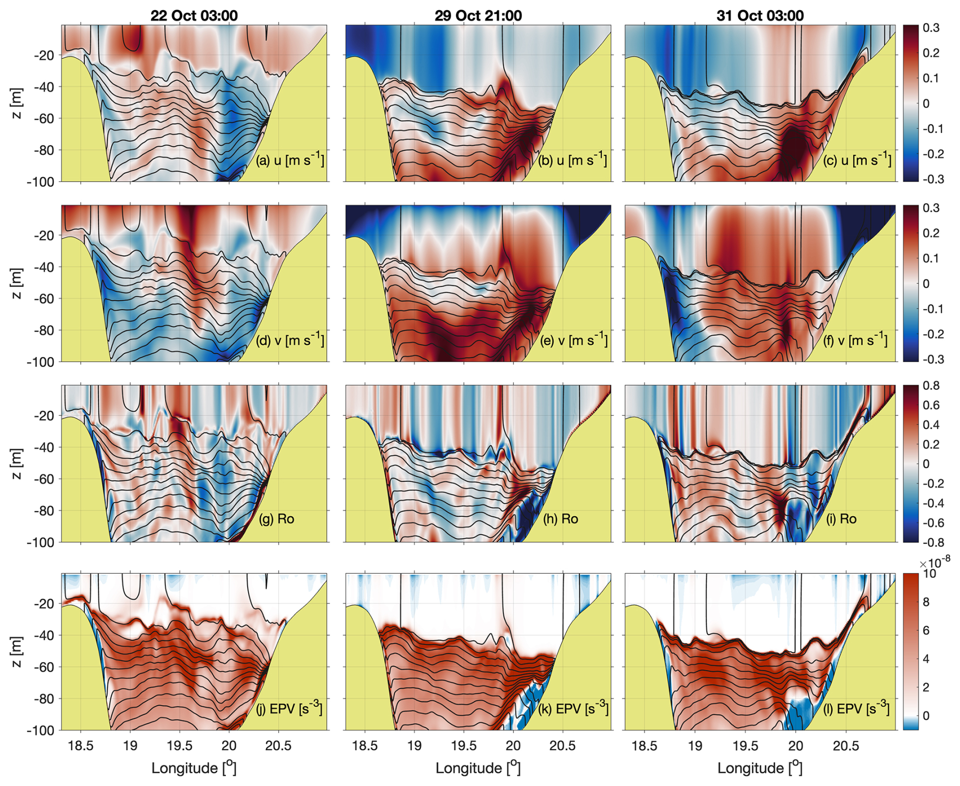
Figure 4 Wind-modulated vorticity generation above sloping topography. Vertical sections of (a–c) across-slope velocity (negative to the left; positive to the right), (d–f) along-slope velocity (negative out of the page; positive into the page), (g–i) Rossby number, and (j–l) Ertel potential vorticity. The location of the transect is shown in Fig. 3 (black continuous line). All panels are instantaneous patterns before (22 October 03:00 UTC, same snapshot as in Fig. 3), during (29 October 21:00 UTC), and at the end of the last storm episode (31 October 03:00 UTC, see also Fig. 2). Black contours in all panels denote isopycnals.

Before the northerly storm (left panels in Fig. 4), the interior flow below the mixed layer is directed southwards. Negative Ro values thus appear at the western boundary, and positive at the eastern boundary (Fig. 4g). Such opposing signs are also found in the EPV, which exhibits highly correlated patterns with Ro (see also Fig. 3). Considering that the strong halocline effectively separates the surface-layer and deep-water processes, the vorticity seen here and the associated submesoscale structures in Fig. 3 are most likely generated by flow-topography interactions rather than surface processes. During these pre-storm conditions with winds from south-easterly direction, the dominance of EPV < 0, indicative of BBL overturning instabilities, implies that the western boundary is a pronounced mixing hotspot (Fig. 4j).

Driven by mostly northerly winds during the storm, however, the direction of the along-slope flow reverses, significantly affecting the vorticity sources and sinks along with the mixing hotspots. Alternating positive/negative BBL vorticity signals, therefore, appear close to the bottom in the snapshots shown in Fig. 4, with the signals intensifying during the severe storm episode. These alternating signals (both in time and between east and west) result from the variability of the along-slope flow, and are thus indirectly linked to the transient nature of the wind field, as shown also further below. At the onset of the storm (Fig. 4e), the strong northerly winds drive a southward flow in the surface layer, inducing a baroclinic return current in the deeper layers. The roughly two-layer flow in the interior and the emergence of coastal jets aligned with the wind direction at both coasts suggest that the flow exhibits features indicative of Ekman dynamics (see Introduction), as described by Krauss and Brügge (1991). Close to the eastern margin, this roughly two-layer flow (more pronounced at the peak of the wind event) generates vorticity with opposite signs above and below the mixed layer (Fig. 4h, around 20–21° E). Thus, opposing vertical vorticities are found not only between the eastern and western sides of the basin, but also between the near-surface and deeper layers below the pycnocline.

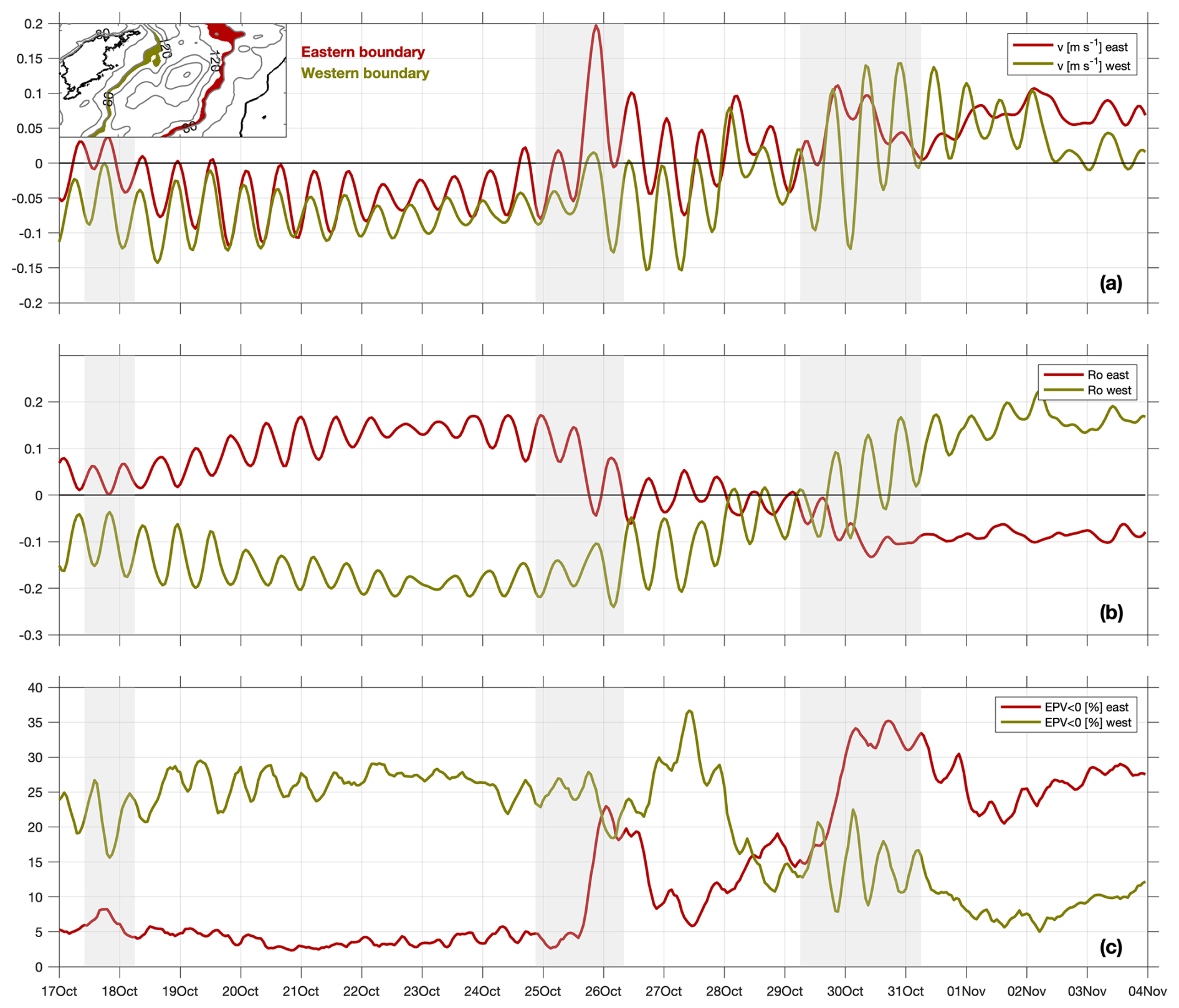
Figure 5 Temporal evolution of vorticity at the lateral boundaries of the basin. (a) Meridional velocity (positive north, into the page) and (b) Rossby number (Ro) at the eastern (red) and western (green) margins of the basin. (c) Fraction of the boundary covered by near-zero and negative Ertel potential vorticity (EPV). The gray shaded areas in all panels indicate the duration of the three successive storm episodes. The inset panel in (a) shows the boundary region, defined as the area between 80 and 100 m depth.

The opposing vertical vorticity signals between the eastern and western boundaries are more clearly illustrated in Fig. 5, which focuses on the near-boundary region. During the first half of the study period, prior to the northerly storm, the dominance of southward along-slope flow (Fig. 5a) results in positive Ro at the eastern boundary, while vorticity of opposite sign develops along the western boundary (Fig. 5b). During the prolonged final storm event, however, the along-slope currents reverse direction, accompanied by a corresponding reversal in the sign of the vorticity, consistent with the snapshots shown in Figs. 4d–i. Such current reversals following wind reversals in the deeper layers have been reported in previous studies, indicating that the circulation rapidly responds to the atmospheric forcing (Liblik et al., 2022; Zhurbas and Väli, 2022; Lips et al., 2026). Note that during the second storm event – characterized by south-southeasterly winds – a predominantly southward interior flow would be expected; however, northward currents are observed along the eastern boundary, likely reflecting the greater wind variability during this event compared to the more persistent northerly winds associated with the final storm. Wind reversals do not necessarily result in an immediate reversal of the current, as the pre-existing flow first needs to adjust to the new wind forcing. The response of Ro therefore depends on the pre-existing flow conditions but also on wind intensity and storm duration. Near-inertial waves are also evident (Fig. 5b), with previous studies (Holtermann and Umlauf, 2012; Holtermann et al., 2014) demonstrating that in our study region they play a relatively minor role in boundary mixing (see Introduction).

Figure 5c further shows the fraction of the near-bottom region occupied by nearly zero and negative EPV. The percentage of low PV, indicative of conditions favorable for overturning instabilities (Garabato et al., 2019), increases substantially at the eastern boundary during storm periods, reaching nearly 30 % at the peak of the final event, while simultaneously decreasing along the western boundary. Such negative PV values can arise under stable stratification when strong anticyclonic vertical vorticity dominates (Gula et al., 2016). Here, the occurrence of negative PV appears to be primarily associated with the direction of the along-slope flow, which, as discussed below, is favorably aligned to trigger downslope Ekman transport, thereby reducing stratification and PV. Overall, Figs. 4 and 5 show that wind reversals frequently followed by current reversals (see also Liblik et al., 2022) can lead to alternate ζ and EPV signals within the BBL, suggesting that the submesoscale generation sites and mixing hotspots exhibit transient behavior. These signals are observed to alternate between the eastern and western sides of the basin and intensify locally during storms.

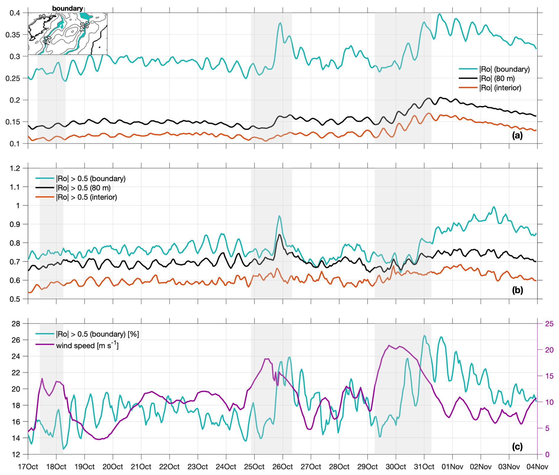
Figure 6 Wind effects on Ro intensity. (a) Absolute value of Ro along the lateral boundaries of the basin (blue line), defined as the region between 80 and 100 m depth (blue shading in the inset panel), at 80 m depth (black line) and in the basin interior excluding the lateral boundary regions (depth > 100 m). (b) Same as in (a) but for strong Ro features (|Ro| > 0.5). (c)  Fraction of the boundary region occupied by ageostrophic features (blue line) and basin-averaged wind speed (purple). Gray shaded areas indicate the duration of the three successive storm episodes.

While Figs. 4 and 5 mainly show that storms are important in regulating the alternating Ro patterns by controlling the direction of the along-slope currents, Fig. 6 more clearly indicates that storms also influence the magnitude of Ro. The time series display the absolute values of Ro (|Ro|) at 80 m depth, in the interior (depth > 100 m), as well as along the lateral boundaries of the basin (Fig. 6a). Consistent with Fig. 4, Fig. 6 exhibits higher |Ro| values during the severe wind events, suggesting that submesoscale structures are generated. When only the strong |Ro| values (|Ro| > 0.5, Fig. 6b) are considered, this storm-driven intensification becomes more evident. |Ro| is higher at the lateral boundaries, further supporting that these areas act as submesoscale generation sites, with the decay time scale for Ro appearing to be of the order of 1 week (see Fig. A1 in the Appendix). Low |Ro| is observed after the second storm event (Fig. 6b), when winds weakened and shifted from southward to northward (Fig. 1c and Fig. A1). This is partly because the winds should first act to decelerate the pre-existing flow before the current can reverse, suggesting that the response to individual wind events also depends on the pre-existing flow conditions. Figure 6 further shows that the |Ro| intensity largely follows the wind variability, albeit with a time lag, especially after wind reversals (e.g., last storm event). By considering only the strong Ro (|Ro| > 0.5), we illustrate in Fig. 6c the fraction of the boundary occupied by such strong ageostrophic features. This fraction clearly increases during storm periods, reaching approximately 27 % during the final storm episode.

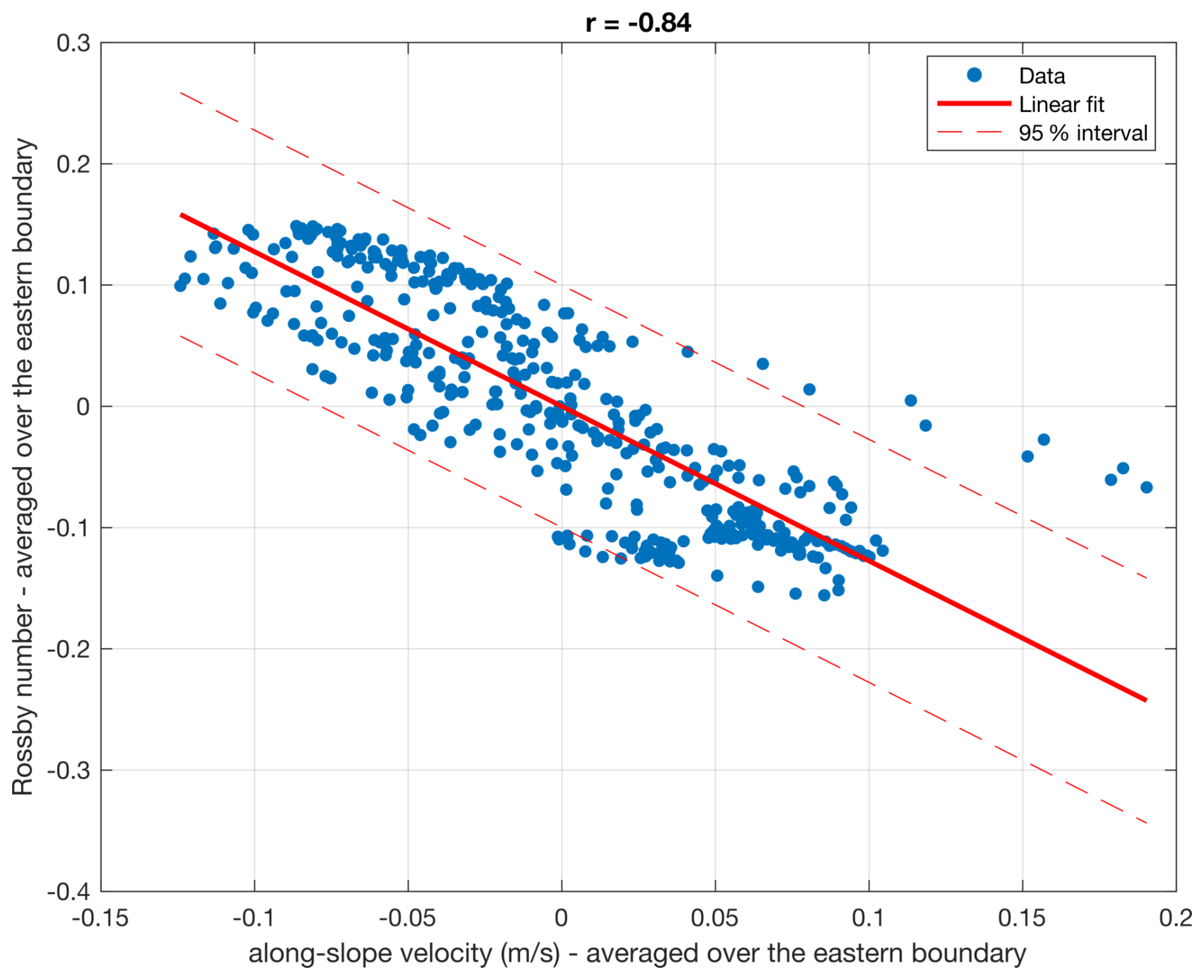
Focusing on the eastern boundary (red region in Fig. 5a) cross-correlation analysis between the along-slope velocity and Ro shows a maximum correlation at zero lag (r = −0.84), confirming that Ro is tightly linked to the current. Consistent with Fig. 5, the negative correlation indicates that the sign and magnitude of Ro follow the direction and strength of the current, becoming increasingly negative as the northward current strengthens and positive when the current is southward (see Appendix, Fig. A2). Moreover, a maximum correlation of r=0.6 at a lag of approximately 13 h was found between Ro at the eastern boundary and the meridional wind component, suggesting that changes in wind forcing are followed by a response in Ro on a timescale comparable to the local inertial period. Note that we use the meridional wind component here because the storm events are predominantly oriented in the north–south direction, and the meridional component is approximately aligned with the alongshore direction at the eastern boundary. Focusing on the entire Eastern Gotland Basin, the wind field and the interior current were strongly correlated (r=0.69) at a lag of 14 h. Similar results were obtained when correlating the current magnitude specifically in the boundary region (blue shading in the inset panel of Fig. 6a) with the magnitude of the meridional wind component (r=0.8, lag = 16 h) and the magnitude of the meridional wind stress (r=0.82, lag = 15 h). Overall, our analyses indicate that storms affect the magnitude and, most importantly, the sign of vorticity – by reversing the interior currents. This reveals a clear dynamical link between wind forcing and near-bottom flow, providing new insights into the dynamics of submesoscale phenomena in wind-driven basins.

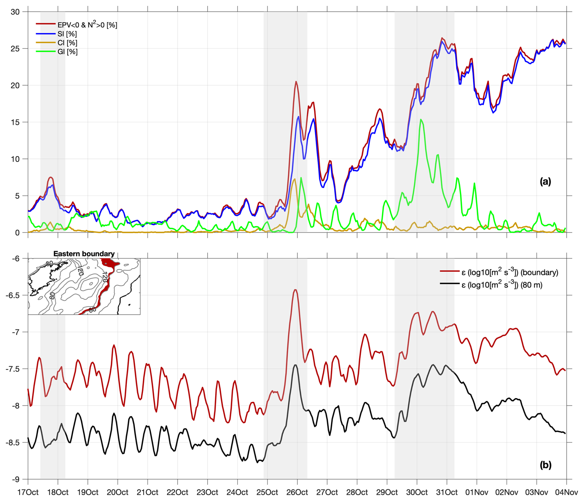
Figure 7 Instability analysis and energy dissipation at the eastern boundary of the basin, defined as the region between 80 and 100 m depth (red shading in the inset panel). (a) Fraction of the boundary that is unstable to symmetric instability (SI, blue line), centrifugal instability (CI, yellow), and gravitational instability (GI, green). The red line indicates the EPV < 0 regions that are, however, gravitationally stable (N²>0). (b) Temporal evolution of dissipation rate, ε, spatially averaged at 80 m depth over the entire domain (black line; including the boundary region shown by the blue shading in the inset panel of Fig. 6a) and over the eastern boundary only (red line; red shading in the inset panel).

6 Storm-forced BBL instabilities

Regions with negative EPV in a sloping BBL indicate that the flow is prone to overturning instabilities. To explore the temporal evolution of the various instability types (see Sect. 2.3), namely gravitational (GI), symmetric (SI), and centrifugal instability (CI), we focus specifically on the eastern boundary of the basin where, as seen in Fig. 5c, the EPV < 0 regions increase substantially during storms. Figure 7a illustrates the fraction of the near-bottom region that is unstable to each instability type. SI (blue line) clearly dominates throughout the entire study period, with the GI (green line) percentages increasing during the two severe wind episodes. The fraction of the domain that satisfies the SI criteria increases significantly during and after the last storm event, reaching approximately 25 %. As briefly discussed below, this effect can be largely traced to a wind-induced reversal of the along-slope currents northward (Fig. 5a, red line), which are downwelling-favorable (i.e., downslope Ekman transport) and therefore support the evolution of SI. The fraction of the domain satisfying the CI conditions remains small (yellow line in Fig. 7a). This may be due to the lack of steep bathymetry, which has been seen to favor CI emergence (Dewar et al., 2015; Wenegrat and Thomas, 2020). It may also be due to the method used here to distinguish between the different instability types. As shown in Sect. 2.3, the applied instability criteria are rather crude and do not consider mixed modes. In the BBL, however, mixed centrifugal-symmetric modes have been seen to dominate (Garabato et al., 2019; Jagannathan et al., 2023). These instabilities trigger vigorous turbulent mixing in the BBL, with the negative PV values typically coinciding with high energy dissipation (Gula et al., 2016). Here, enhanced energy dissipation rates are observed along the basin boundary (Fig. 7b), and they intensify substantially during storms, pointing to a dynamical association with the low-PV regions.

7 Summary and Conclusions

We have used a realistic high-resolution simulation to explore the genesis of interior submesoscale phenomena in a semi-enclosed, predominantly wind-driven basin and to elucidate the impact of storm events on deep-water submesoscale dynamics. Focusing on the central basin of the Baltic Sea, we find that a wealth of filamentary and eddy-like features populate the basin's interior, below the main pycnocline. To the best of our knowledge, these interior structures have not been investigated previously in the Baltic Sea, with existing studies (e.g., Carpenter et al., 2020; Chrysagi et al., 2021; Lips et al., 2026) focusing primarily on submesoscale activity in the surface mixed layer. Our results show that surface and subsurface submesoscales can coexist while remaining largely decoupled from each other. As storm-intensified currents interact with the sloping bottom, anomalies in relative vorticity and EPV are generated through frictional and diabatic processes within the BBL (Benthuysen and Thomas, 2012; Wenegrat and Thomas, 2020). These strong vorticity anomalies are subsequently exported from the boundary into the stratified interior in the form of eddies, fronts and filaments, which are inherently submesoscales and act to facilitate the boundary-interior exchanges. The latter provides a missing link connecting the observation of enhanced boundary mixing in the Baltic Sea with the finding that boundary mixing determines basin-scale deep-water mixing, which implies a connection between the BBL and the interior region (Holtermann and Umlauf, 2012; Lappe and Umlauf, 2016).

The most energetic submesoscale features appear during storms, with wind forcing indirectly modulating these motions by altering the interior circulation. Strong correlations are found between wind forcing and deep-water circulation, as well as between Ro and along-slope flow. Such along-slope flows may be either directly wind-driven, as described by Krauss and Brügge (1991), or indirectly mediated by near-inertial and topographic waves (Holtermann and Umlauf, 2012; Holtermann et al., 2014), or different types of seiching motions (Zakharchuk et al., 2021). By analyzing a series of sequential storm events with opposing winds, we also found that variability in wind direction is important in determining both the submesoscale generation sites and the mixing hotspots, which in turn exhibit transient behavior. Wind reversals reverse the currents, generating oppositely-signed ζ and EPV in the BBL, with EPV < 0 indicating conditions favorable to overturning instabilities (Garabato et al., 2019). In addition to wake instabilities arising in the lee of topography due to flow–topography interactions (Molemaker et al., 2015; Dewar et al., 2015; Gula et al., 2015), such overturning instabilities can also develop within the BBL due to cross-slope Ekman transport induced by along-slope currents (Garabato et al., 2019; Wenegrat and Thomas, 2020; Jagannathan et al., 2023). These instabilities typically occur when the along-slope flow is favorably aligned (i.e. with the coast on its right in the Northern Hemisphere) to trigger downslope Ekman transport, such that lighter fluid is advected beneath denser fluid, leading to boundary layer thickening, enhanced mixing, and reduction of PV (Moum et al., 2004; Benthuysen and Thomas, 2012; Umlauf et al., 2015). This is consistent with Figs. 3–5, which show enhanced PV destruction, particularly when the storm-intensified along-boundary flow is downwelling-favorable.

One of the key findings of our study is therefore that intense and variable winds can strongly influence interior submesoscale dynamics. Storms not only modulate the strength of submesoscales by altering the intensity of along-slope currents, but they also generate alternating BBL mixing hotspots (both in time and between the eastern and western sides of the basin) by continuously shifting the direction of the interior currents. Such wind-induced current reversals (Krauss and Brügge, 1991; Lehmann and Myrberg, 2008), leading to alternating mixing hotspots, are likely to occur in other marine and limnic systems where circulation is primarily driven by transient wind events, but they are generally not expected in major current systems where the flow direction is predominantly steady. Nevertheless, the main dynamical mechanisms described here are broadly consistent with previous studies that examined similar submesoscale features, albeit in the open ocean, particularly in regions where energetic, steady currents flow over steep topography (Gula et al., 2015; Molemaker et al., 2015; Zhu et al., 2024).

The Baltic Sea, largely unexplored in terms of interior submesoscale dynamics, provides a natural laboratory for studying these processes in a semi-enclosed, wind-driven basin. Most of the dynamical mechanisms identified here are not unique to the Baltic, suggesting that our findings may be broadly applicable to other semi-enclosed, wind-driven marine basins, such as the Black Sea and Caspian Sea, as well as large limnic systems like the Great Lakes and Lake Geneva. In Lake Geneva, submesoscale motions have recently been observed in the surface layer (Hamze-Ziabari et al., 2022), while strong boundary mixing – potentially linked to submesoscale instabilities – has been detected in the interior by glider measurements (Sepúlveda Steiner et al., 2023).

For the Baltic Sea, future work could assess the influence of the slope Burger number (Bu) in modulating the occurrence of negative EPV along the basin's boundaries. As Bu in the Baltic Sea varies broadly and often abruptly, idealized modelling work (e.g., Masini et al., 2025), including sensitivity experiments with different slopes and stratification conditions, could shed light on the nature of instabilities (Wenegrat et al., 2018) that emerge as wind-driven flows interact with sloping boundaries.

In conclusion, our work shows that variable wind forcing over sloping basin boundaries can generate a rich field of submesoscale motions via a breadth of dynamical pathways. These pathways include many canonical scenarios such as topographic wakes and instabilities within the BBL considered by past theoretical and idealised modeling studies, while extending the range of topographic and ambient flow conditions in which submesoscales may develop. This result suggests that intense and variable wind forcing over sloping topography can be particularly effective in promoting near-boundary mixing, energy dissipation, and boundary-interior exchange, and calls for an investigation of our findings' generality to other transient wind-driven basins.

Appendix A: Response of vertical vorticity to wind events

Although a detailed description of the effects of storms on Ro is provided in Sect. 5, the study period – corresponding to a field campaign – is relatively short. Hence, to illustrate the broader impact of storms on Ro magnitude during autumn, a two-month time series is shown in Fig. A1. A relatively moderate increase in |Ro| is observed during wind events, followed by a gradual decay over a time scale of one week. Consistent with Fig. 6, higher Ro values are found near the lateral margins of the basin, where submesoscales are generated, with |Ro| peaking during the 30 October storm event (Fig. A1b). The |Ro| variability is, however, relatively low, suggesting that submesoscales might be active most of the time. This might be further related to the stormy season examined here, as the successive storm events and the overall strong winds (Fig. A1a) helped to sustain generally elevated |Ro| values.

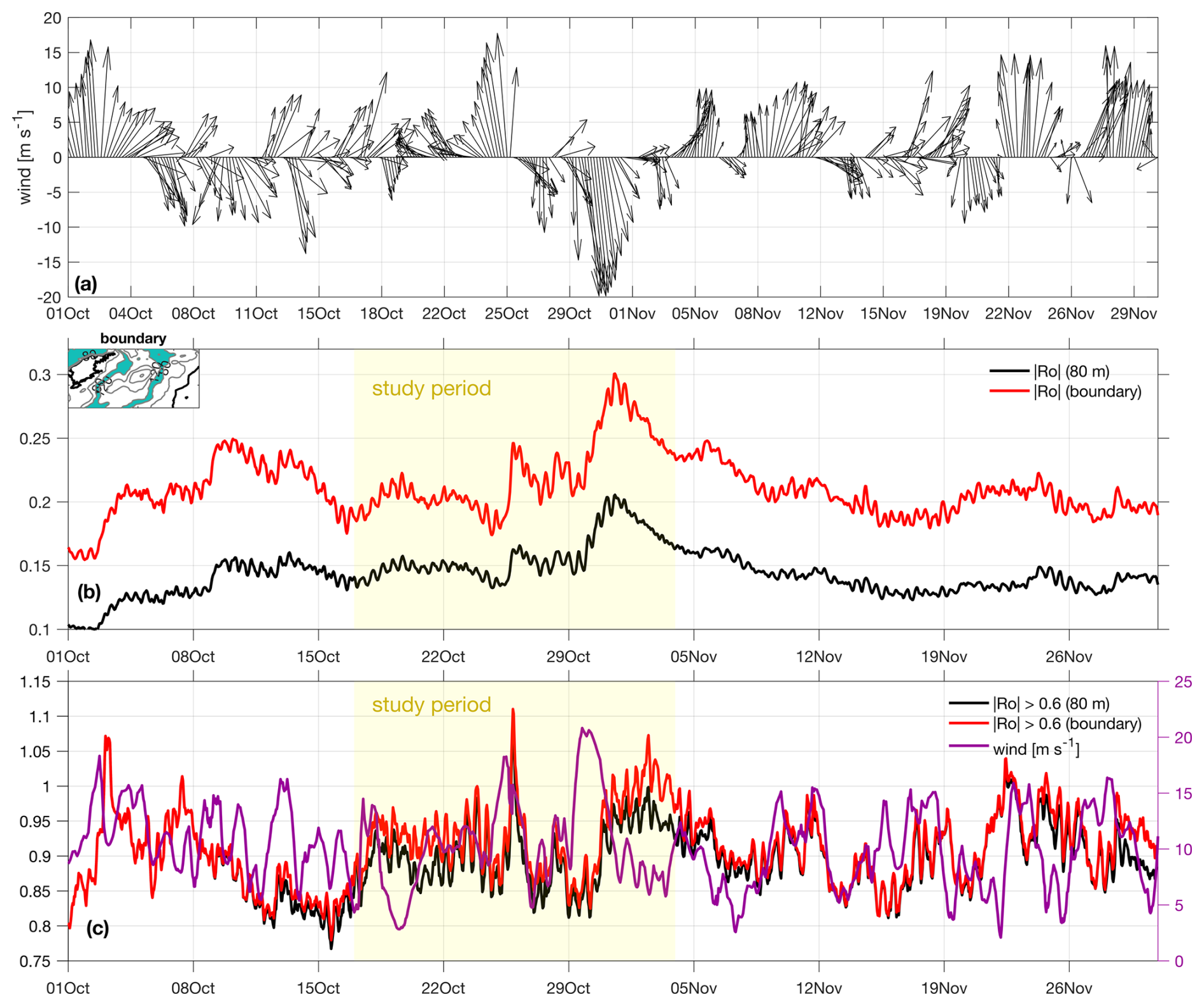
Figure A1 (a) Basin-averaged wind speed and direction, (b) absolute value of Ro at 80 m depth (black line) and near the lateral boundaries of the basin (red line), defined as the area between 80 and 120 m depth (green region in the inset panel). (c) Same as before, but for the strong Ro features (defined as |Ro| > 0.6). The purple line indicates the spatially averaged wind speed. The study period is indicated by the light yellow shaded area.

The impact of storms on the magnitude of vorticity is more pronounced when only the strong |Ro| values (|Ro| > 0.6, Fig. A1c) are considered, with the deep-water Ro significantly increasing when the wind increases. Nevertheless, continuous shifts in wind direction strongly affect the |Ro| intensity, leading to reduced vorticities even under relatively strong winds. This is evident, for example, during 9–17 October, when |Ro| decreased substantially (Fig. A1c) despite the moderately high wind speeds (Fig. A1a). Overall, Fig. A1 shows, as in Fig. 6, that |Ro| largely follows the wind variability, albeit with a time lag, especially after wind reversals (e.g., the 30 October storm episode). Wind reversals do not necessarily result in an immediate reversal of the current, as the pre-existing flow first needs to adjust to the new wind forcing (e.g., following the 25 October wind event). The response of Ro therefore depends on the pre-existing flow conditions but also on wind intensity and storm duration.

Focusing on the eastern boundary of the basin (red shaded area in Fig. 5a), cross-correlation analysis between the along-slope velocity and Ro (Fig. A2) yields a maximum of r = −0.84 at zero lag, demonstrating a strong inverse relationship between Ro and the along-slope flow. Stronger northward flow (v>0) is associated with increasingly negative Ro, and vice versa, in agreement with Figs. 3–5. This behavior is consistent with numerous studies (Molemaker et al., 2015; Gula et al., 2015, 2016) showing that flow–topography interactions can generate either anticyclonic or cyclonic relative vorticity, depending on the direction of the interior flow relative to the coast (see Introduction).

Figure A2 Correlation between along-slope velocity and Ro at the eastern boundary of the basin (red shaded area in Fig. 5a).