Decadal biogeochemical predictions for the changing bottom marine environment of the Gulf of Maine

The Gulf of Maine and the surrounding Northeast US Continental Shelf are experiencing rapid marine environmental change arising from complex regional dynamics that challenge near-term (1–10 years) predictive capabilities for valuable living marine resources. Here, using a high-resolution regional ocean model, we demonstrate skilful decadal forecasts of ocean bottom habitat characteristics including bottom temperature, dissolved oxygen (O₂), pH and aragonite saturation state (Ω_ar). Bottom temperature and pH predictions show substantial skill driven primarily by radiatively forced change and carbon uptake trends, while bottom O₂ and Ω_ar predictions benefit more from initialization due to stronger internal variability. Retrospective forecasts successfully predicted observed historical changes in water masses and environmental properties, including recent cooling/freshening transitions driven by replacement of Warm Slope Water with Labrador Slope Water. This water mass variability also modulates biogeochemical conditions and ocean acidification buffering capacity, with our recent forecasts indicating that benefits from the expected respite from rapid warming might be tempered by challenges posed by rapid acidification. The demonstrated predictability of coupled physical-biogeochemical processes supports developing integrated prediction systems for climate-informed marine resource management.

1 Introduction

The global ocean has undergone unprecedented biogeochemical transformation since the onset of the industrial era – absorbing approximately 30 % of anthropogenic CO₂ emissions, and over 90 % of the excess heat associated with accumulating greenhouse gases (Sabine et al., 2004; Feely et al., 2023, Friedlingstein et al., 2025, Johnson and Lyman, 2020). This oceanic CO₂ and heat uptake has initiated a cascade of interconnected changes that represent some of the most profound shifts in ocean conditions experienced in the past 50 years. Warming has altered ocean stratification and circulation (Levitus et al., 2012; Abram et al., 2016). Acidification has challenged the basic chemistry upon which marine calcifiers depend (Caldeira and Wickett, 2003; Orr et al., 2005). Declining oxygen concentrations have pressed the metabolic limits of marine organisms (Keeling et al., 2010; Breitburg et al., 2018). Ecosystem and fisheries challenges posed by climate change are compounded by those linked to natural climate variability (Lehodey et al., 2006). A capacity to anticipate physical and biogeochemical changes, whether from climate change or natural variability, may help coastal communities and industries mitigate potential negative impacts, and realize new opportunities that may arise (Clark et al., 2001; Tommasi et al., 2017b).

The Northeast US Continental Shelf (NEUS) – and particularly its highly productive semi-enclosed sea, the Gulf of Maine (GOM) – has been subject to both ocean change trends and pronounced variability. Dynamic warming (Pershing et al., 2015; Saba et al., 2016; Alexander et al., 2018), deoxygenation (Claret et al., 2018) and acidification (Salisbury and Jönsson, 2018; Siedlecki et al., 2021; Stewart et al., 2025) signals have emerged from an interplay of shifting circulation patterns, alterations in the Gulf Stream position, and regional water masses, particularly variations between cold, fresh Labrador Slope Water (LSW) and Warm Slope Water (WSW) associated with greater Gulf Stream influence, that modulate global warming signals through local oceanographic processes (Chen et al., 2020; Gangopadhyay et al., 2019; Brickman et al., 2018; Gonçalves Neto et al., 2021; Friedland and Hare, 2007; Seidov et al., 2021). In the GOM, oceanic variability from interannual to longer time scales is understood to be largely driven by changes in the contributions of these and other source waters which, in turn, modify the temperature, salinity, and nutrient conditions across the entire ecosystem (Mountain, 2012; Townsend et al., 2023). This water mass variability has also generated complex and sometimes counterintuitive local biogeochemical responses to climate change, including an influx of high-alkalinity Gulf Stream waters driving increased buffering to acidification in certain areas despite rising atmospheric CO₂ concentrations (Stewart et al., 2025; Salisbury and Jönsson, 2018). Such water mass changes may also influence coastal hypoxia risk by altering stratification patterns that control vertical mixing and oxygen dynamics in coastal bottom waters (Scully et al., 2022).

Rapid warming of the GOM has already contributed to the decline of its iconic Atlantic cod fishery and triggered cascading ecosystem changes (Pershing et al., 2015, 2021; Hare et al., 2016). Continued warming, deoxygenation, and acidification pose significant threats to commercially important fisheries, particularly American lobster and shellfish. American lobsters show stage-specific vulnerabilities to acidification and warming that vary significantly between regional populations (Harrington and Hamlin, 2019; Niemisto et al., 2025). Early life stages of shellfish consistently show greater sensitivity to acidification than adults, creating recruitment bottlenecks that may drive population declines (Fay et al., 2017). Impacts extend beyond commercially harvested species to affect protected species such as Atlantic puffins and northern right whales (Meyer-Gutbrod et al., 2021).

Decisions by coastal communities and managers that determine long-term resource and community resilience are made across time horizons and must consider both variability and change. The interannual to decadal time horizon (1–10 years) is particularly notable for its relevance to the setting of annual catch limits, the formulation of stock rebuilding plans, and industry capitalization (Tommasi et al., 2017b). Global Earth System Models (ESMs) have demonstrated multiyear predictability for surface temperature, pH, dissolved oxygen, and net primary production, and enhanced subsurface predictability extending to a decade in the North Atlantic where Atlantic Meridional Overturning Circulation (AMOC) variability strongly influences physical drivers (Frölicher et al., 2020; Krumhardt et al., 2020; Park et al., 2019; Msadek et al., 2014). This ocean predictability enables predictability of the distribution of commercially important open-ocean fish species in the North Atlantic over decadal time scales (Payne et al., 2022).

Fisheries are concentrated on productive and accessible continental shelves, however, where direct applications of global ESMs are limited by coarse spatial resolution (∼100–200 km) that cannot adequately represent the complex bathymetry, coastal dynamics, tidal mixing, and mesoscale circulation features that drive ocean and ecosystem variability on the shelf (Tommasi et al., 2017b; Saba et al., 2016; Ross et al., 2023). High-resolution ocean modeling and enhanced observational networks are revealing substantial promise for predicting ocean variability in this highly dynamic region (Gehlen et al., 2015; Ross et al., 2023, 2024; Chen et al., 2021, 2024; Koul et al., 2024).

In the GOM (Fig. 2a), recent observations show cooler, fresher water entering the deeper regions through the Northeast Channel beginning in late 2023, potentially marking the return of cooling LSW influence after over a decade of warm Gulf Stream dominance (Record et al., 2024). Previous work regional ocean prediction studies demonstrated that this physical transition, and others like it, were predictable (Koul et al., 2024). Such shifts, however, also have significant biogeochemical implications, as LSW offers lower buffering against acidification than Gulf Stream water. If the recent cooling represents a sustained return to LSW dominance, the region could face rapid acidification as the reduced buffering will compound ongoing background acidification trends (Salisbury and Jönsson, 2018; Stewart et al., 2025). Such rapid biogeochemical change could challenge marine ecosystems and shellfish industries adapted to a decade of warm yet less acidic conditions.

Here, we build on prior physical ocean prediction studies and present a high-resolution regional physical and biogeochemical prediction system that, when used to downscale global decadal predictions (Delworth et al., 2020), addresses this time-critical challenge by capturing both the physical and biogeochemical dynamics of shifting water masses and persistent change. We furthermore shift the focus of the evaluation to the benthic environment, which is critical for the largest and most lucrative Gulf of Maine fisheries (e.g., lobster, scallops and groundfish, Waller et al., 2023). Through a comprehensive 10-member ensemble approach spanning 60 years of initialized retrospective predictions, accompanied by uninitialized simulations that include only the impacts of external radiative forcings (∼6500 years of simulations), we demonstrate skilful decadal (1–10 year) predictions of benthic physical and biogeochemical conditions in the Gulf of Maine. Our experiments allow us to isolate the impacts of radiatively forced ocean warming on prediction skill, and the impacts of predictable water mass variations. Finally, we present probabilistic forecasts for the coming years that may offer fisheries managers actionable insights into the near-term trajectory of the benthic environment in the GOM.

Table 1 Overview of the three types of downscaled experiments presented in this study, focusing on the differences between the experiments.

2 Methods

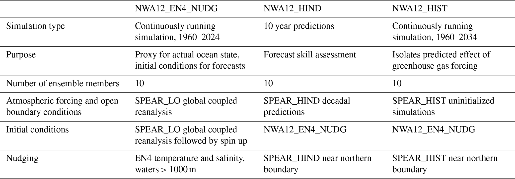
Several sets of regional ocean simulations were used to study the predictability of physical and biogeochemical changes in the Gulf of Maine. These are summarized here and in Table 1 to provide a broad view of the experiment structure. Further details of each component are then provided in the subsections that follow.

First, a large set of 10-member ensemble retrospective decadal (10-yearlong) forecasts, or “hindcasts”, were generated starting each January from 1965 to 2025 by downscaling ensemble predictions from the coarse resolution Seamless System for Prediction and EArth System Research (SPEAR) decadal prediction system (Delworth et al., 2020; Yang et al., 2021) to the $\mathrm{1}/\mathrm{12}$° Northwest Atlantic (NWA12) regional ocean model of Ross et al. (2023). These predictions, which comprise nearly 6500 years of simulation, are referred to herein as NWA12_HIND, and the global SPEAR hindcasts used to force them are referred to as SPEAR_HIND.

NWA12_HIND hindcasts were initialized with a 10-member ensemble of retrospective NWA12 simulations forced by the same SPEAR ensemble reanalysis used for SPEAR_HIND (Yang et al., 2021). The regional runs were furthermore nudged gently toward the EN4 in waters > 1000 m. These simulations, which will also aid in prediction analysis, are referred to as NWA12_EN4_NUDG.

Finally, an ensemble of simulations of the historical effects of climate change drivers (increasing greenhouse gases, aerosol changes, land use) was generated by downscaling the historical and early projection period of an ensemble of SPEAR climate change simulations. Unlike the predictions in NWA12_HIND and SPEAR_HIND, these climate change runs were not initialized from a data constrained ocean state, but from alternative states from the SPEAR pre-industrial control simulation. The mean of this ensemble is used to estimate the signal associated with climate change, or the “forced” signal, over natural variations. These runs are referred to as “NWA12_HIST” to indicate that they are derived from the historical portion of a climate change simulation. They are also referred to as “uninitialized” runs to indicate that, unlike predictions that aim to anticipate both climate variations and change, they are not initiated from a data-constrained initial state.

2.1 The $\mathrm{1}/\mathrm{12}$° regional MOM6-COBALT-NWA12 model

The regional downscaled model developed here inherits most of the configuration and parameters from the MOM6-COBALT-NWA12 v1.0 model developed by Ross et al. (2023) and further refined for applications to decadal predictions by Koul et al. (2024). The model comprises coupled components for ocean physics, biogeochemistry, and sea-ice. Compared to the previously published decadal predictions, we add the COBALT biogeochemical model (Stock et al., 2020, 2025) and improve the initial physical state estimates by relaxing the downscaled simulation towards the EN4 dataset (Good et al., 2013) at depth greater than 1000 m.

2.2 The global SPEAR model

We use a 10-member SPEAR-based global simulation (SPEAR_LO; Delworth et al., 2020; Yang et al., 2021) with a low-resolution configuration (1° ocean and sea ice with near-equatorial refinement; and 1° atmosphere and land) to obtain surface forcing and open boundary conditions for the regional model. We use forcing and boundary conditions from the SPEAR_LO global coupled reanalysis to create the NWA12 simulations used to initialize our hindcasts (i.e., NWA12_EN4_NUDG, Table 1), and forcing from SPEAR hindcasts (SPEAR_HIND) to drive NWA12_HIND. For the SPEAR_LO reanalysis, atmospheric winds and temperature were restored toward the 6-hourly Japanese Reanalysis (JRA3Q; Kosaka et al., 2024), and the oceanic SST is restored toward the interpolated monthly-mean observations from the NOAA Extended Reconstructed Sea Surface Temperature version 5 (ERSSTv5) dataset (Huang et al., 2017). The reanalysis ensemble spread originates through alternative deep ocean initializations and is maintained due to the gentle surface-only assimilation approach used by SPEAR_LO (Yang et al., 2021).

2.3 Regional downscaled simulation (NWA12_EN4_NUDG)

SPEAR_LO reanalysis output was used to force the regional MOM6 model at the ocean surface and at the three open ocean boundaries (see Koul et al., 2024) from January 1960 to December 2024. The 10 members of this regional downscaled simulation (NWA12_EN4_NUDG) are derived from the 10 members of the SPEAR_LO: we simply carry forward the member-wise information present in the ocean initial conditions, atmospheric forcing and open ocean boundary conditions.

The interior solution of the NWA12_EN4_NUDG simulation was furthermore relaxed with a 90 d timescale towards the full vertical profiles of ocean temperature and salinity from the EN4 gridded dataset in regions where the ocean bottom is deeper than 1000 m. This moderate relaxation helps keep the model solution closer to the observation-based sub-surface variability, particularly in the late 1990s when the boundary conditions overestimated the propagation of a cool, fresh signal into the domain. Limiting the relaxation to waters deeper than 1000 m helps avoid rapid oceanic re-adjustment in shallower waters upon initialization of retrospective predictions wherein such relaxation towards EN4 is not carried out and is necessary to avoid nudging on the shelf where the 1° EN4 shows low correlation with observed salinity despite maintaining high correlation with observed temperature (Figs. S2 and S3). We also note that the bottom waters of the Gulf of Maine analysed in this study (the deep basins and the Northeast Channel) lie well inshore of the 1000 m isobath and are therefore not directly nudged towards EN4. The relaxation constrains only the off-shelf slope source waters. We do not relax the regional model towards the parent SPEAR model, since SPEAR has coarse ocean resolution and does not assimilate sub-surface ocean data, making it less constrained towards observations than the EN4-gridded dataset.

Open boundary data for biogeochemical tracers were obtained exactly as explained in Ross et al. (2023). The time varying boundary data for alkalinity and dissolved inorganic carbon were estimated from SPEAR_LO monthly average temperature and salinity as input to the algorithm from Carter et al. (2021). Climatological river freshwater discharge, nutrient, carbon and alkalinity data were also used as described in Ross et al. (2023) and Koul et al. (2024). This climatological forcing, which includes seasonal variability but not interannual variability, was used because coastwide river observations dating back to the 1960s are not available. In the Gulf of Maine, direct river runoff is estimated to be a minor source of freshwater and nutrients (Smith et al., 2001; Townsend, 1998) and most of the interannual variability is driven by changing sources of inflowing water.

2.4 Regional ocean hindcasts (NWA12_HIND)

Following Koul et al. (2024), we use the regional simulation from the NWA12_EN4_NUDG model to start 10-yearlong retrospective ocean physical-biogeochemical predictions (NWA12_HIND) every year on 1 January from 1965 to 2025. The last 10-yearlong simulation, which shifts from hindcast to forecast, is from 1 January 2025 to 31 December 2034. The 10-member NWA12_HIND ensemble are started from ocean initial conditions taken from the corresponding 10 members of NWA12_EN4_NUDG, and integrated forward using atmospheric forcing and open ocean boundary conditions from the 10 members of SPEAR_HIND. To ease the transition between the global and regional model of the complex inflow and outflow along the northern boundary, each member of the 10-yearlong predictions is relaxed towards the corresponding SPEAR_LO prediction north of 45° N. The strength of the restoration corresponds to a relaxation time scale of 90 d at the northern boundary and decreases gradually to 0 at 45° N. No bathymetric mask is applied, as the relaxation drops to zero north of the targeted shallower regions. The latitudinal damping rate r (inverse of relaxation time scale) was prescribed as:

$$\begin{array}{}\text{(1)}& r\left(\mathit{\varphi }\right)=\left(r_{\max }/\mathrm{2}\right)\times \left[\mathrm{1}+\cos \left(\mathit{\pi }\left({\mathit{\varphi }}_{\max }-\mathit{\varphi }\right)/\left({\mathit{\varphi }}_{\max }-\mathrm{45}\right)\right)\right]\end{array}$$

for ϕ (latitude) from 45° N to ϕ_max in the regional model, and zero south of 45° N and $r_{\max }=\mathrm{1}/\mathrm{90}$ d⁻¹ at ϕ_max, where ϕ_max in the regional model is ≈58° N.

2.5 Historical climate change simulations (NWA12_HIST)

The NWA12_HIST is a continuous 75-yearlong simulation started on 1 January 1960 and ending in 31 December 2034. The NWA12_HIST is also a 10-member ensemble forced with atmospheric forcing and open ocean boundary conditions from the 10 members of SPEAR_HIST. The SPEAR_HIST dataset spans from 1850 to 2100 and incorporates future greenhouse gas concentrations based on the SSP585 emissions scenario (Riahi et al., 2017). It should be noted that differences between SSP585 and other emissions scenarios are negligible over the near future (next 1–10 years) examined in this study. Both NWA12_HIST and NWA12_HIND share the response of the model to the common prescribed natural and anthropogenic radiative forcing but the phase of natural variability in NWA12_HIST is not expected to match the observed phase since the impact of 1960 initial conditions is not retained beyond a few years.

2.6 Point observations and observation-based gridded products

Two observation-based gridded data sets were used to assess the quality of model simulations for bottom temperature and salinity: the $\mathrm{1}/\mathrm{12}$° GLORYS12 v1 ocean reanalysis and interim analysis products (Lellouche et al., 2018) and the 1° EN4 gridded dataset (EN.4.2.2, Good et al., 2013) which is used to assess a longer period from 1965–2024 (Fig. S1 in the Supplement, Figs. 3 and 5). For bottom O₂ and bottom Ω_ar, we used the Fishing Industry SHared Bottom Oceanographic Timeseries data (https://erddap.ondeckdata.com/erddap/tabledap/fishbot_realtime.html, last access: 29 May 2025), hereafter called “Fishbot”, and vessel (Jiang et al., 2021) and glider-based (IOOS Glider Data Assembly Center: https://gliders.ioos.us/erddap/index.html, last access: 29 May 2025) datasets (hereafter called “NOAA OBS”). In addition to these two datasets, we also used the observed bottom temperature and bottom salinity time series (hereafter called “NOAA_SOE”) for the GOM Ecological Production Unit (EPU) from NOAA's State of the Ecosystem reports (NOAA Fisheries, 2025).

2.7 Preparation of annual mean anomalies

Area-weighted averages were first computed for the model-simulated ensemble mean and the two gridded observational datasets (GLORYS12 and EN4), excluding grid cells with ocean depths less than 30 m. Annual anomalies were then derived by subtracting the 1994–2023 mean from the annual mean time series. Figures S1–S3 show the comparison of annual anomalies from variables across these gridded datasets.

For all Fishbot and NOAA_OBS observations, point data was first linearly interpolated onto a uniform $\mathrm{1}/\mathrm{4}\mathit{°}\times \mathrm{1}/\mathrm{4}\mathit{°}$ grid before area averaging. Monthly anomalies were then computed by subtracting the long-term monthly mean (1994–2023) from each month, provided there were at least three years of data samples. Finally, annual mean anomalies were calculated by averaging monthly anomalies for years with at least four months of data. The uncertainty (error bars in Fig. 2) for that year is σ_monthly/$\sqrt{n}$, i.e. the sample standard deviation of that year's monthly anomalies divided by the square root of the number of valid months (n).

2.8 Gulf Stream index and water mass definitions

The variability of the Gulf Stream's position was assessed using a method established by Pérez-Hernández and Joyce (2014) and subsequently utilized by Ross et al. (2023). First, the Gulf Stream's mean position is defined by the latitude where sea surface height (SSH) variance is highest along meridional lines, spaced 1° apart, from 72 to 52° W. Then, to quantify the relative position of the Gulf Stream, the Gulf Stream Index (GSI) was calculated as the annual SSH anomaly, relative to the 1994–2023 average, averaged over these mean position points. The proportion of the two water masses, Labrador Slope Water and Warm Slope Water, in the Northeast Channel (Fig. 1) analyzed in this study were computed from water mass definitions as described in Ross et al. (2023).

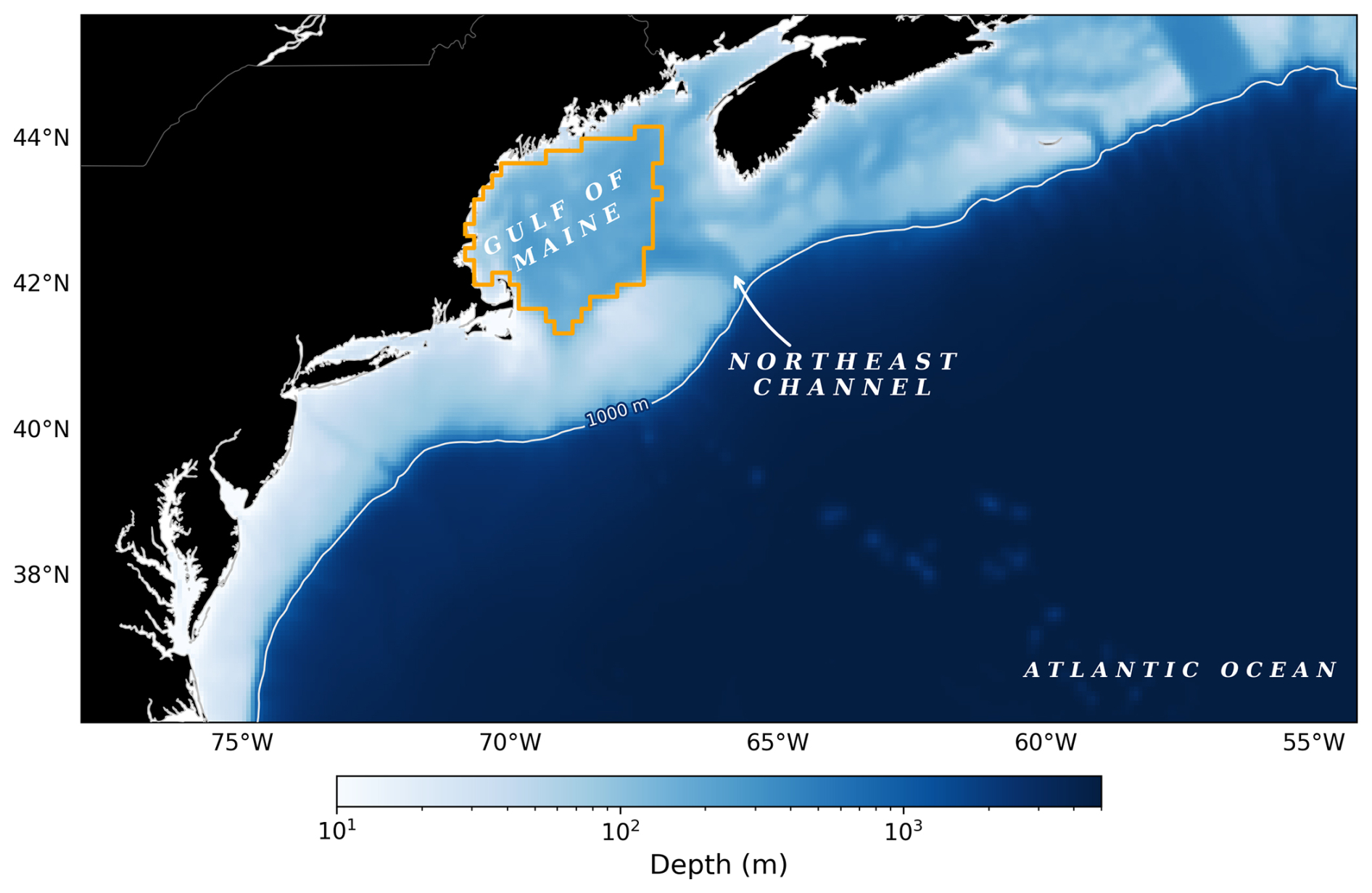
Figure 1 The study region and its characteristics. The locations of the Gulf of Maine Ecological Production Unit (GOM_EPU) and the Northeast Channel along the Northeast US continental shelf are shown along with the model bathymetry and the 1000 m isobath (white line).

2.9 Skill assessment

We used anomaly correlation coefficients (ACC) to quantify the skill in predicting annual mean anomalies of bottom temperature, bottom O₂, bottom pH and bottom Ω_ar. The ACC for area-averaged quantities was calculated for the Gulf of Maine Ecological Production Units (GOM_EPU, NOAA Fisheries, 2024). For bottom temperature, bottom O₂, bottom pH and bottom Ω_ar the NWA12_EN4_NUDG simulation was used as the observational reference, and the skill was calculated over the period 1965–2024. The lead-dependent climatology (1994–2023 mean) was removed from the initialized hindcasts before calculating the skill metric. This choice of using NWA12_EN4_NUDG as the observational reference was made because continuous spatio-temporal observational records of bottom temperature, O₂, pH and bottom Ω_ar, for any of the EPUs or Large Marine Ecosystems (LMEs) were not available. However, to show that the NWA12_EN4_NUDG was a good proxy for in-situ observations for the skill estimation, we carried out a point-by-point comparison of temporally and spatially co-located model output and available observations (Fig. S7), as well as additional evaluation of interannual variations and covariance with better-constrained physical properties (Figs. S1, 3 and 5). A simple persistence-based skill, defined as the lagged autocorrelation of observed anomalies, was also compared with the hindcast skill.

We assessed the statistical significance of the prediction skill from the initialized NWA12_HIND retrospective predictions. This was done by conducting a two-tailed t-test against a null hypothesis of no correlation, adjusting for the reduced degrees of freedom due to autocorrelation. Additionally, we compared this skill to that of persistence forecasts and the uninitialized (NWA12_HIST) simulation. For this comparison, we employed the Williams (1959) method as described in Steiger (1980) to determine the statistical significance between two dependent correlation coefficients.

2.10 Prediction probabilities and their skill

Probabilistic tercile predictions are developed by post-processing the model forecasts using extended logistic regression (Wilks, 2009). Extended logistic regression fits the probability of the outcome y exceeding a certain threshold q given some data x, and is formulated as

$$\begin{array}{}\text{(2)}& P\mathit{\{}y>q|x\mathit{\}}=\mathit{\sigma }(f\left(x\right)+g\left(q\right))\end{array}$$

where the logistic function $\mathit{\sigma }\left(z\right)=\mathrm{1}/(\mathrm{1}+e^{-z})=e^z/(\mathrm{1}+e^z)$. Here, f is a simple linear function of the ensemble mean prediction x: $f\left(x\right)={\mathit{\beta }}_{\mathrm{0}}+{\mathit{\beta }}_{\mathrm{1}}\cdot x$, and the extension function g is also a simple function of the threshold q: $g\left(q\right)={\mathit{\beta }}_{\mathrm{2}}\cdot q$. Maximum likelihood estimation, following Minka (2001) and Pregibon (1981), is used to fit the three beta parameters for each of the four forecast variables in Fig. 7. In this method, the forecast probability is a function of only the ensemble mean, and not the individual ensemble members or the ensemble spread. As is common in seasonal to decadal dynamical model predictions, we find that the raw ensembles tend to be overconfident, with insufficient ensemble spread (Fig. S8). Furthermore, the ensemble spread has low correlation with the actual retrospective forecast error. As a result, extended logistic regression provides a reasonable improvement to the estimates of the forecast uncertainty.

For evaluating probabilistic predictions, we use accuracy as the verification metric for each tercile. The accuracy is calculated as:

$$\begin{array}{}\text{(3)}& \begin{array}{rl}\mathrm{Accuracy}& =(\mathrm{True}\mathrm{Positives}+\mathrm{True}\mathrm{Negatives})\\ & /\mathrm{Total}\mathrm{Forecasts}.\end{array}\end{array}$$

This metric is computed independently for each tercile category. In this context, a true positive occurs when the tercile with the highest predicted probability correctly matches the observed tercile. A true negative occurs when the model correctly assigns the highest probability to either of the other two terciles (effectively predicting that observations will not fall within the tercile being evaluated).

We also calculated the ranked probability skill score (RPSS) for each variable to assess the accuracy of the predictions across all three categories. Persistence of the previous year's category was used as the reference for the RPSS, so positive skill scores indicate that the model forecasts have some ability to predict transitions away from recent conditions.

The RPSS is a skill score based on the Ranked Probability Score (RPS), and the Ranked Probability Score (RPS) for a single forecast is defined as

$$\begin{array}{}\text{(4)}& \mathrm{RPS}={\displaystyle \frac{\mathrm{1}}{K-\mathrm{1}}}\sum _{k=\mathrm{1}}^K{\left[\sum _{i=\mathrm{1}}^k{P}_i-\sum _{i=\mathrm{1}}^k{O}_i\right]}^{\mathrm{2}}\end{array}$$

where K is the number of categories (3 in our case: below, normal, or above), P_i is the cumulative forecast probability for category i, and O_i is the cumulative observed probability (0 or 1) for category i. A perfect forecast, which assigns 100 % probability to the observed category, will have an RPS = 0. Predicting a 100 % chance of the opposite outcome (i.e., below when the outcome is above) gives an RPS of 1, while predicting normal when an outcome is above gives an RPS of 0.5. The RPS is notable in that it evaluates the distribution of the forecast probability around the outcome, penalizing outcomes that are further away. This makes RPS a more sensitive metric than accuracy.

The ranked probability skill score (RPSS):

$$\begin{array}{}\text{(5)}& \mathrm{RPSS}=\mathrm{1}-\mathrm{RPS}\left(\mathrm{forecast}\right)/\mathrm{RPS}\left(\mathrm{persistence}\right)\end{array}$$

where RPS (forecast) is the sum of the ranked probability scores comparing the forecast probabilities with the observed categories, and RPS (persistence) is the sum of the ranked probability scores comparing the observed categories with the categories observed in the previous year (in other words, we assign 100 % probability to the category observed in the year before the forecast was initialized, and compare that with the actual category for the next 3 years). By the definition of the skill score, if RPSS = 1, the forecasts had perfect accuracy at probabilistically predicting the observations. If RPSS = 0, the forecasts had the same overall score as the persistence forecasts of the previous year's state; in other words, the forecasts would have had no skill at predicting transitions.

2.11 Decomposition of the drivers of bottom O₂ alkalinity and aragonite saturation state (Ω_ar)

Bottom O₂ saturation ([O₂] sat), was computed from the simulated bottom potential temperature and salinity following Garcia and Gordon (1992). DIC and alkalinity were not saved at the ocean bottom and were thus obtained by solving the carbonate system (PyCO2SYS; Humphreys et al., 2022) from the model's bottom pH and Ω_ar together with bottom temperature and salinity at a representative pressure of 150 dbar. The result is largely insensitive to this pressure choice – recomputing Ω_ar from the recovered DIC and alkalinity reproduces the simulated Ω_ar to within 0.01. COBALT additionally applies minor nutrient alkalinity corrections (PO₄ and SiO₄) that are omitted here, with negligible effect on the bottom anomalies.

The contributions of bottom DIC, alkalinity, temperature (T) and salinity (S) to the bottom pH and Ω_ar anomalies were quantified by perturbing each variable in turn about the 1994–2023 mean state; the contributions sum to the total to within 0.0045 in pH and 0.008 in Ω_ar. To attribute their anomalies, we used a one-factor-at-a-time perturbation about a fixed reference state defined as the 1994–2023 climatological mean of each driver, (DIC₀, Alk₀, T₀, S₀). The reference values pH₀ and ${\mathrm{\Omega }}_{{\mathrm{ar}}_{\mathrm{0}}}$ were obtained by solving the carbonate system at that state.

Four perturbation time series were constructed to estimate the contribution of each driver to interannual pH and Ω_ar anomalies by allowing a single driver to take its full annual-mean value while the other three were held fixed at their climatological mean. The approximate contribution of each driver to the pH (or Ω_ar) anomaly in year t is then the departure of its perturbed solution from the reference. For example, $\mathrm{\Delta }{\mathrm{pH}}_{\mathrm{DIC}}\left(t\right)=\mathrm{pH}\left(\mathrm{DIC}\right(t),{\mathrm{Alk}}_{\mathrm{0}},T_{\mathrm{0}},S_{\mathrm{0}})-{\mathrm{pH}}_{\mathrm{0}}$.

Because the carbonate system is non-linear, the four single-driver contributions are not guaranteed to add up exactly to the total anomaly; the difference is the residual cross-term arising from simultaneous variation of two or more drivers. In practice this residual is negligible here: the sum of the DIC, alkalinity, T and S contributions reproduces the full bottom pH and Ω_ar anomalies to within 0.0045 pH units and 0.008 in Ω_ar over the whole record.

3 Results and discussion

3.1 Bottom temperature and salinity

The regionally downscaled retrospective simulations, NWA12_EN4_NUDG, which were used to initialize retrospective forecasts, have an ensemble mean that matches the complex patterns of bottom warming and cooling in the GOM (Fig. 2a). The period from the 1980s to the mid-1990s shows a gradual warming of about 2 °C followed by cooling of the same magnitude until mid-2000s, and intensified warming from the mid-2000s to around the year 2020. This bottom variability in the regional downscaled simulations is consistent with the observed long term surface temperature variations that the Northwest Atlantic Ocean has experienced over the past century, which have been characterized by distinct multi-decadal oscillations and dramatic shifts in water mass properties that have shaped marine ecosystems from the Labrador Sea to Cape Hatteras (Wallace et al., 2018; Townsend et al., 2006; Mountain, 2012). In the late 1990s, after a long period of persistent presence of Warm Slope Water (WSW), cold and fresh Labrador Slope Water (LSW) replaced WSW along the Scotian Shelf and GOM (Drinkwater et al., 1998; Mountain, 2004; Friedland and Hare, 2007). WSW increased in prevalence again during the period from 2004 to 2020 in conjunction with an unprecedented era of accelerated surface and bottom warming in the Northwest Atlantic, making it one of the fastest-warming ocean regions globally (Pershing et al., 2015; Friedland et al., 2020; Kavanaugh et al., 2017; Du Pontavice et al., 2023). Real-time Fishing Industry SHared Bottom Oceanographic Timeseries (Fishbot) data and independent observation-based datasets (Figs. 2a, S1 and S2; see also Record et al., 2024) suggest that the rapid warming has paused since the early 2020s, as predicted by earlier simulations with the downscaled regional model (Koul et al., 2024), and markedly cooler water has returned to the region in 2024.

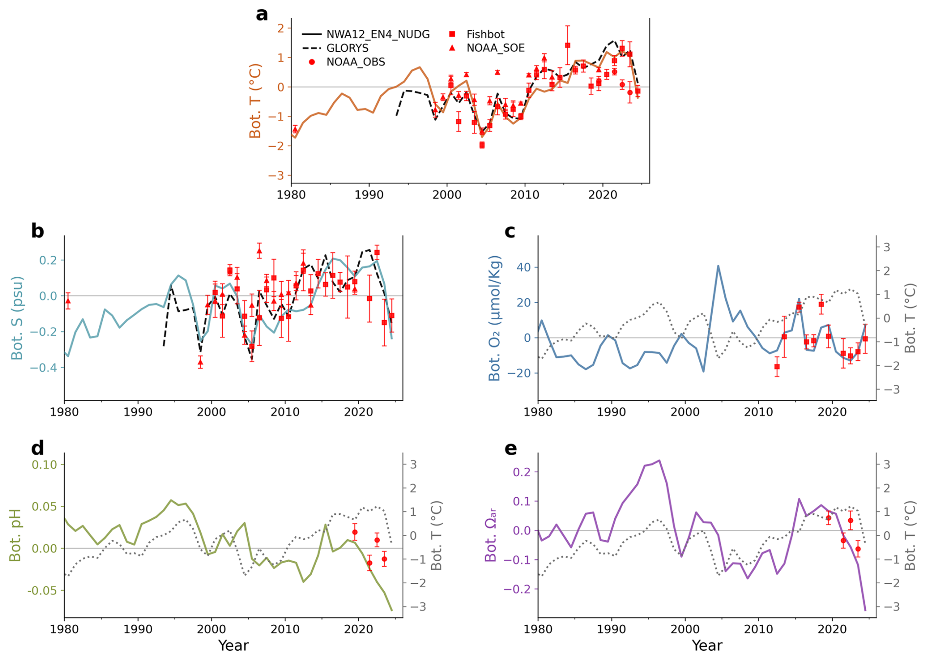
Figure 2 Physical and biogeochemical variability in the GOM. Annual mean anomalies of (a) bottom temperature (°C), (b) bottom salinity (psu), (c) bottom oxygen (µmol kg⁻¹, (d) bottom pH and (e) bottom aragonite saturation state in the GOM from the ensemble mean of the regional downscaled simulations (NWA12_EN4_NUDG, colored solid lines) and observations (markers with error bars). Observations from the NOAA SOE reports (NOAA_SOE, triangles), the Fishbot bottom data (squares) and the aggregated point observations from vessels and gliders (NOAA_OBS, circles) are also shown for available years. The error bars depict the uncertainty of the annual mean (see Sect. 2). The dashed black lines in (a) and (b)  re from the GLORYS12 dataset. All anomalies are calculated with respect to the 1994–2023 mean. To highlight physical and biogeochemical co-variability, bottom temperature lines are shown as dotted grey lines in (c)–(e).

Simulated bottom salinity closely tracks bottom temperature variability (Figs. 2b and S3; r=0.84); noticeable differences are only seen at the shorter interannual time scales. The correlation between temperature and sparse bottom salinity observations (NOAA_SOE) is weaker but also positive (r=0.58). However, confounding from seasonal and spatial variability limits the inference of annual average salinity anomalies from the sparsely observed salinity field alone. The independent GLORYS12 bottom temperature and salinity estimates, which use a high-resolution model with data assimilation to impute estimates within the spatial and temporal gaps between observations, are highly correlated with our simulation results over the shorter GLORYS record (r=0.86 and r=0.70, respectively) – and have a similarly strong bottom temperature and bottom salinity covariance (Figs. 1b and S3, r=0.84 versus r=0.90).

3.2 Bottom oxygen, pH and aragonite saturation ratio

The water mass variations described above are also accompanied by biogeochemical shifts in both the model and observations (Fig. 2c–e). The annual mean bottom oxygen (O₂) anomalies in the GOM show an inverse relationship with bottom temperature and salinity anomalies. The warming and water mass transitions described above would be expected to influence dissolved oxygen concentrations through differences in O₂ concentration in water masses (Claret et al., 2018), solubility effects, and potential changes in biological oxygen demand. The rise in deep oxygen levels from the mid-1990s, peaking in the latter half of 2004 to 2005, corresponds with the cool, fresh, high LSW conditions well documented in the observational record (Mountain, 2012; Feng et al., 2016). LSW is high in oxygen due to high solubility and rapid oxygen uptake during its formation in the Labrador Sea (Koelling et al., 2023). Since 2005 the bottom oxygen levels have largely dropped, aside from episodic increases in 2015, 2019, and 2024. The relationship between internal (natural) variations in bottom temperature and bottom O₂ confirms that the proportion of WSW/LSW in the Northeast Channel acts as an important driver of this co-variability, though meteorologically linked variations in the winter mixed layer also dictate large episodic variations in bottom O₂ (Figs. 5 and S5). The close correspondence between the observed Fishbot data and the modeled bottom O₂ (Fig. 3c) suggests that our regional downscaled simulation captures the dominant mechanisms controlling bottom oxygen variability.

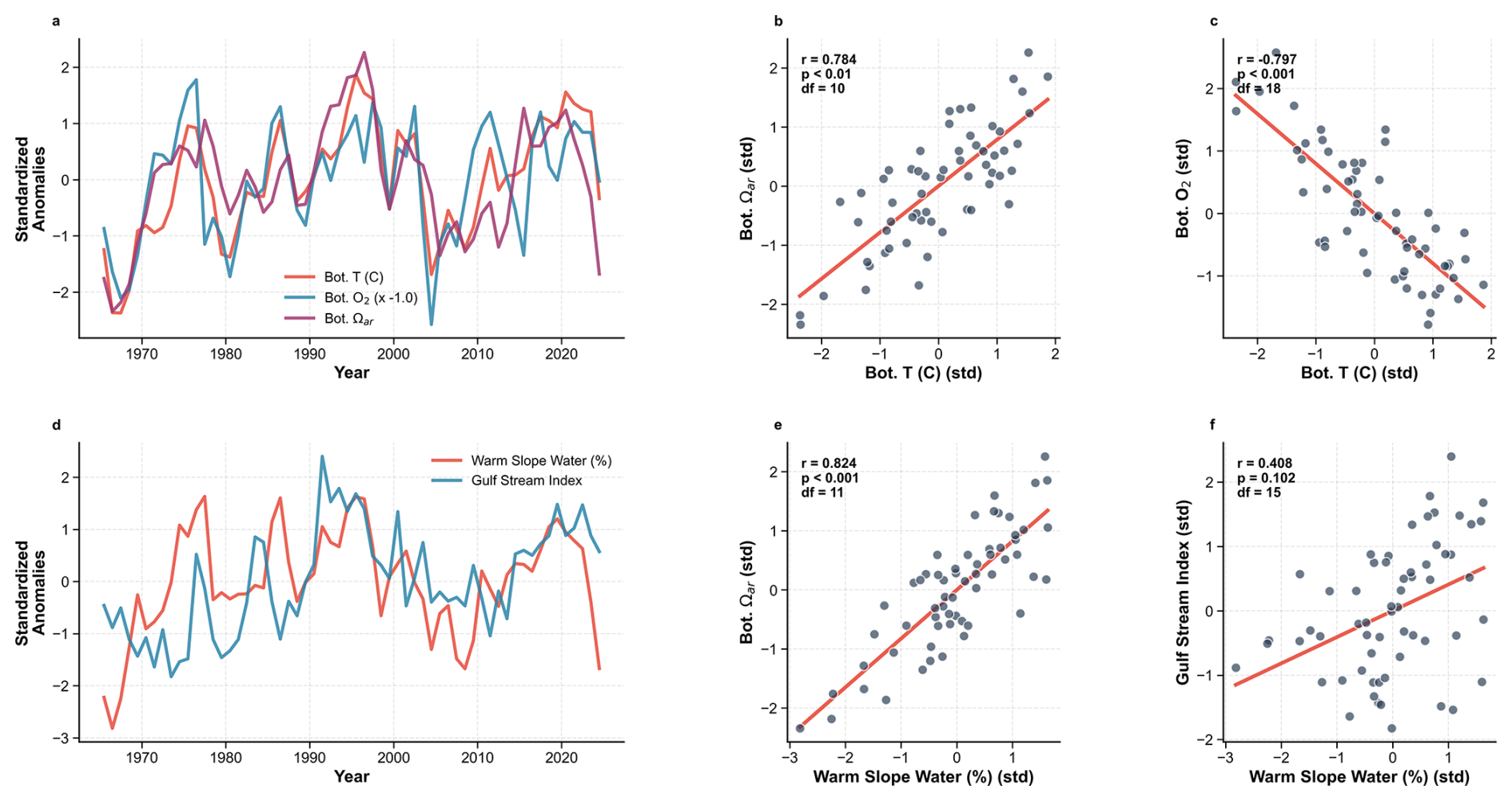
Figure 3 Drivers of internal co-variability in the GOM. Standardized anomalies (with respect to 1994–2023 period) of the internal (natural) component of the annual mean (a) bottom temperature, bottom O₂ and bottom Ω_ar in the GOM, (b) percentage of warm slope water (WSW) in the Northeast Channel and the Gulf Stream Index from the regional downscaled simulations. Also shown are scatterplots of internal components of (c) bottom temperature and bottom Ω_ar, (d) bottom temperature and bottom O₂, (e) WSW and bottom Ω_ar and (f) WSW and the Gulf Stream Index, along with the linear regression fit (red line). The Pearson correlation coefficient (r), the associated p value and the degrees of freedom (df) are also provided for each pair of variables. The internal component is the difference between the ensemble mean of the downscaled simulation (NWA12_EN4_NUDG) and the ensemble mean of the uninitialized downscaled simulations (NWA12_HIST). The bottom oxygen in (a) is multiplied by −1.0 to show its covariability with bottom temperature.

The bottom pH and aragonite saturation state (Ω_ar) anomalies in the GOM show an overall declining trend from 1980–2024 consistent with the uptake of steadily increasing atmospheric CO₂ (i.e., predictable large-scale ocean acidification). The simulated Ω_ar time-series, however, also exhibits more significant inter-annual to decadal variability than the bottom pH (Fig. 2d and e), which is consistent with Salisbury and Jönsson (2018). After removing the externally forced ocean acidification signal, Ω_arvariations are positively correlated with temperature (Fig. 3, r=0.75). This is consistent with the carbonate chemistry response to warming and increased alkalinity in warm and saline WSW waters (Salisbury and Jönsson, 2018). As in Salisbury and Jönsson's surface analysis, the pronounced warming and shift to WSW from 2010–2020 was associated with increased Ω_ar that counteracted the ocean acidification trend seen in pH. The more recent shift toward colder and fresher conditions, however, amplifies the acidification trend and causes a sharp decrease in Ω_ar.

3.3 Drivers of bottom biogeochemical variability

To isolate the mechanisms underlying this bottom biogeochemical variability, we decomposed each quantity into its controlling factors (Fig. 4). Bottom O₂ was partitioned into a solubility component, the saturation concentration [O₂] sat (T, S), and a non-solubility residual, [O₂] − [O₂] sat, which equals the negative of the apparent oxygen utilisation (− AOU) and reflects ventilation, respiration and advection (Fig. 4a). The non-solubility residual accounts for approximately 70 % of the interannual variance of the bottom-O₂ anomaly (r=0.89 with total O₂), compared with about 21 % for the solubility term. The dominant O₂ variations – including the episodic maxima of 2004, 2015 and 2019 – are therefore driven by ventilation of the deep basins through deep winter mixing (Fig. S5) and by the changing oxygen content of the inflowing slope waters, rather than by temperature and salinity-dependent solubility alone. Solubility instead imparts a smaller, smoother decline as the bottom water warms.

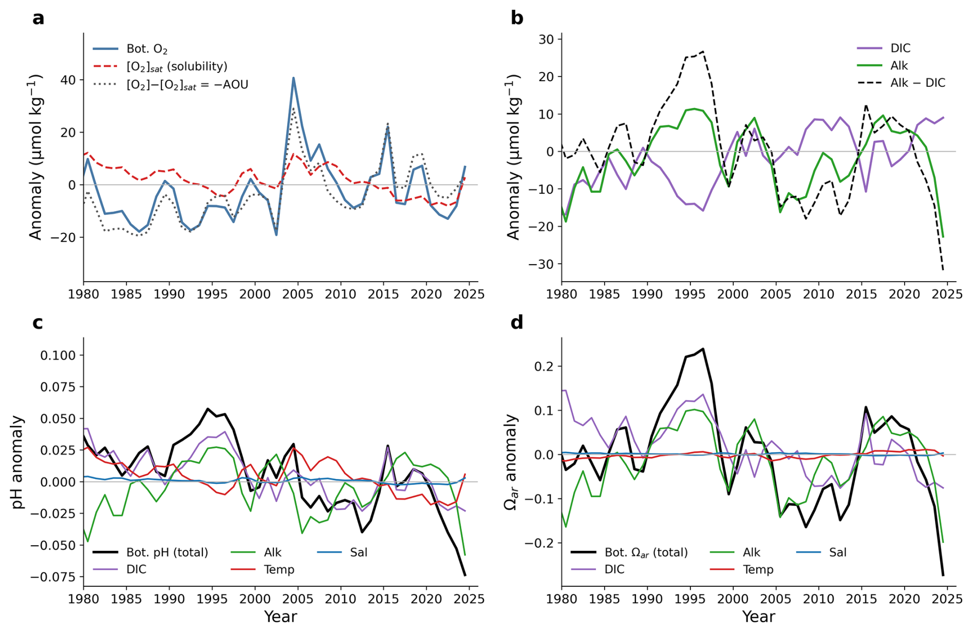
Figure 4 Decomposition of bottom-water biogeochemical variability in the Gulf of Maine. (a) Bottom-O₂ anomaly partitioned into the solubility term [O₂] sat and the non-solubility residual [O₂] − [O₂] sat (≈ − AOU) in the NWA12_EN4_NUDG retrospective simulation (ensemble mean anomalies relative to 1994–2023). (b) Bottom dissolved inorganic carbon (DIC), total alkalinity (Alk) and Alk − DIC. (c, d) Attribution of the bottom (c) pH and (d) Ω_ar anomalies to DIC, Alk, temperature and salinity, obtained by perturbing each driver about the 1994–2023 mean state; the black line is the total anomaly (see Sect. 2).

For the carbonate system, we examined the bottom dissolved inorganic carbon (DIC) and total alkalinity, which mix conservatively and respond in straightforward ways to gas exchange, respiration and CaCO₃ cycling. We also examine alkalinity minus DIC (Alk − DIC), a proxy that helps separate the mechanisms driving pH and Ω_ar (Xue and Cai, 2020; Fig. 4b). In the model the Alk − DIC anomaly is nearly identical to the bottom Ω_ar anomaly (r=0.996; Fig. 4b and d) but tracks pH relatively loosely (r=0.82, because pH also responds directly to warming). On interannual timescales Alk − DIC (and hence Ω_ar) is set by water-mass alkalinity changes, while its long-term decline (−2.2 µmol kg⁻¹ per decade), rising DIC outpacing a smaller alkalinity increase, is the anthropogenic acidification trend.

We attributed the bottom pH and Ω_ar anomalies to DIC, alkalinity, temperature and salinity (Fig. 4b–d; see Sect. 2). Bottom DIC rises steadily at about 4 µmol kg⁻¹ per decade, which is the likely fingerprint of anthropogenic carbon uptake. Alkalinity varies primarily with water mass, being higher during the high-alkalinity WSW phases and lower during Labrador Slope Water phases (Fig. 4b). The long-term pH decline (−0.013 per decade) is led by the rising DIC (−0.010 per decade), with warming contributing a further −0.007 per decade, increasing alkalinity partially buffering the trend (+0.005 per decade), and salinity making up a small remainder (−0.001 per decade) (Fig. 4c). The decline is thus quantitatively consistent with anthropogenic DIC uptake, modulated by warming and water-mass alkalinity.

The long-term Ω_ar decline (−0.015 per decade) is likewise led by rising DIC, whose direct effect (−0.035 per decade) is more than halved by two opposing influences: increasing alkalinity (+0.016 per decade) and warming (+0.004 per decade) (Fig. 4d). Warming thus raises Ω_ar even as it lowers pH, which, together with the larger water-mass alkalinity signal, is why the Ω_ar decline is weaker and less monotonic than that of pH. On interannual timescales, Ω_ar variability is instead governed primarily by alkalinity (about 57 % of the detrended variance; r=0.91 with the alkalinity contribution), with only a minor direct thermodynamic effect of temperature. The interannual DIC anomaly is small and, because the inflowing WSW in the model does not carry elevated DIC (detrended DIC–alkalinity correlation $r=-\mathrm{0.28}$), the DIC signal slightly reinforces rather than opposes the alkalinity-driven variability (Fig. 4d). The correlation between Ω_ar and temperature (Fig. 2) therefore arises largely because temperature and alkalinity co-vary through the WSW/LSW water-mass variability, rather than from a direct effect of warming on the carbonate equilibria. Bottom salinity, which co-varies strongly with bottom temperature through the WSW/LSW water-mass variations (Figs. 2a, b, and S3), is retained as an explicit driver of the pH and Ω_ar anomalies in this decomposition (Fig. 4c and d), where its direct contribution is small.

3.4 Prediction skill

Decadal prediction skill is derived from both predictable internal variability of the climate system and from predictable natural and anthropogenic external forcing (Meehl et al., 2009). Capturing the latter requires skillful representation of external drivers (e.g., accumulating CO₂) and its impact on the climate, while capturing the former requires skillful initialization of the climate system and the ability to simulate its natural evolution from that state. The analysis in Figs. 2 and 3 suggested that our retrospective ensemble hindcasts (NWA12_HIND) captured observed variations and covariations across bottom habitat properties, and that the prominence of externally forced and internal variability varies between critical bottom habitat quantities. Comparison of extensive retrospective forecasts against these patterns show that some aspects of both signals were successfully predicted, but others were not (Fig. 5).

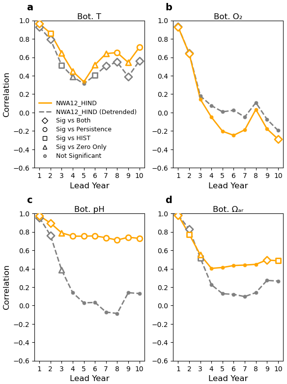
Figure 5 Decadal prediction skill. Anomaly correlation coefficient of the annual mean anomalies from the initialized regional downscaled model (NWA12_HIND) predictions. The symbols indicate statistically significant differences relative to alternative models of no correlation, persistence, and the uninitialized (historical) simulation (see Sect. 2). The correlation is calculated against the regional downscaled simulation (NWA12_EN4_NUDG)-derived annual mean anomalies (ensemble mean) for (a) bottom temperature, (b) bottom O₂, (c) bottom pH and (d) bottom Ω_ar over the GOM_EPU. The prediction and persistence skills are calculated for the common 1965–2024 period. The grey dashed lines show skill for the linearly detrended annual mean anomalies.

Bottom temperature predictions from NWA12_HIND exhibit significant positive anomaly correlations in most of the 10 lead years (Fig. 5a); and in the first lead year, the prediction skill exceeds the skill from the climate change signal (indicated by the diamonds and squares). Both results are consistent with a predictable bottom-temperature signal from climate change and contributions from predictable bottom-temperature (i.e., water mass) variability in the first few lead years. Closer inspection of the prediction skill after linear de-trending further supports the system's capacity to predict aspects of variability around the climate change trend over all the lead years, except at lead years 4 and 5 when the skill drops (Fig. S9). The prediction skill is robust when verified against GLORYS as the observational reference for the period 1993–2024 (Fig. S4).

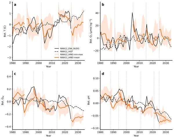
Initializations at states far from the uninitialized state, the 1980s warming, the rapid 2005–2015 warming and the recent shift to cooler/fresher conditions from 2020 onward, are all correctly predicted by the retrospective predictions (Fig. 6). The 2025 forecast shows a slow reversal of the recent cooling/freshening during the next decade. These results could be interpreted as the model simply relaxing toward the uninitialized state. However, the overall good correlation skill indicates that the model accurately captures the timing and magnitude of such transitions.

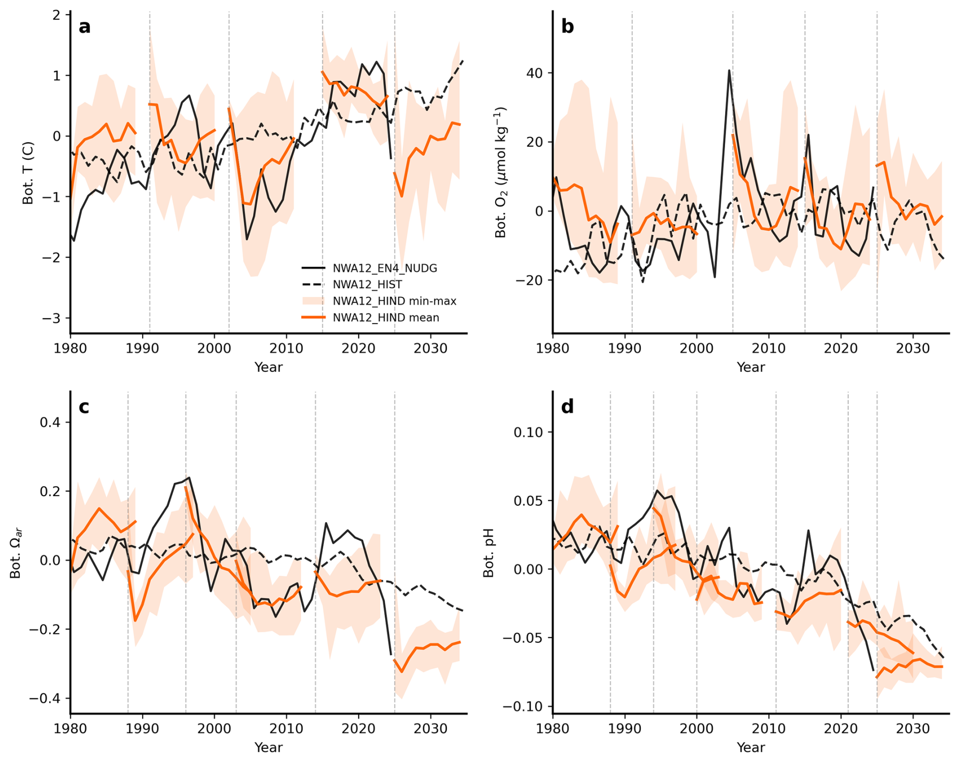
Figure 6 Physical and biogeochemical predictions in the GOM. Annual mean anomalies of (a) bottom temperature (°C), (b) bottom oxygen (µmol kg⁻¹), (c) bottom aragonite saturation state and (d) bottom pH in the GOM_EPU. The solid black lines show the anomalies from the ensemble mean of regional downscaled simulations (NWA12_EN4_NUDG, as in Fig. 2), the dashed black lines show the ensemble mean of uninitialized downscaled model simulations (NWA12_HIST) carried under historical anthropogenic forcing and SSP585 emissions scenario. The bold orange lines show the 10-yearlong initialized prediction (NWA12_HIND) and the vertical grey lines depict their year of initialization. The bold orange lines are the ensemble means of the respective 10-member ensemble, and the light shading is the min-max range of the ensemble members. A lead-time-dependent climatology was removed from each ensemble member to create anomalies. All anomalies are calculated with respect to the 1994–2023 mean.

The prediction skill for bottom O₂ drops to 0 beyond 2 years and much of the signal for this important habitat factor is linked to predictable internal (natural) variability (Fig. 5b). This is also apparent from the time series (Fig. 2c) which shows that bottom O₂ does not have a uniform long-term trend as was the case for bottom temperature. The rapid drop in prediction skill may also be linked to the presence of sharp and likely less predictable meteorologically driven variations in the depth of the winter mixed layer. The winter 2003/2004 is a prime example of this phenomenon when large positive winter MLD anomalies in our regional downscaled model drove ventilation of the bottom water and strong positive bottom oxygen anomalies (Figs. 6, and S5). Similar peaks in bottom O₂coinciding with deep winter mixing and positive MLD anomalies are seen in 2015 and 2019.

The decadal predictions initialized before and after the 2004 peak (in 2002 and 2006 respectively) show that the ensemble mean prediction has difficulties predicting the extent of the rise in bottom O₂, but the subsequent decay of these elevated bottom O₂ levels is well predicted by the model (Fig. 6b). These characteristics of the past variability in bottom O₂ are consistent with the high skill of the initialized predictions, which outperform the persistence-based skill and the skill of uninitialized simulations in the first two lead years (Fig. 5b), and the significant drop thereafter.

Both bottom pH and Ω_ar exhibit a declining trend (Fig. 2e and f), yet they differ in how much the climate change signal influences their prediction skill. Ocean pH is primarily controlled by increasing atmospheric CO₂, while Ω_ar is more strongly influenced by ocean water masses with varying alkalinity (LSW versus WSW). As a result, internal variability contributes more to the prediction skill of Ω_ar, whereas the climate change signal has a greater impact on the prediction skill of bottom pH (Fig. 5c and d). Beyond lead year 2, the climate change signal predominantly determines the prediction skill of bottom pH, allowing it to remain high and significantly better than persistence for all lead years (except lead year 3) which is not the case for Ω_ar where the skill drops rapidly beyond lead year 2. When the linear trend is removed, the skill of internal variability significantly surpasses the persistence and climate change-driven skill in the first two lead years. The notable decrease in the prediction skill of detrended bottom pH, compared to Ω_ar, further demonstrates the additional contribution of internal variability to the prediction skill of Ω_ar. Individual 10-year forecasts provide further evidence of the capability of the model to track past deviation of bottom pH and Ω_ar from the long-term trend (Fig. 6c and d).

3.5 Probabilistic predictions

The preceding analyses leveraged over 6500 years of retrospective forecasts to assess the capacity of the ensemble mean prediction to anticipate physical and biogeochemical changes on a decadal time horizon. While results suggested significant capability arising from predictable climate variability and change signals, decision-making benefits from actionable information on uncertainties (e.g., Ramos et al., 2013; Roulston et al., 2006). A coastal resource manager or fishing industry representative might ask, “How reliable are forecasts for anomalously warm or cool conditions?”. To quantify this in more accessible terms, we calculated the accuracy of probabilistic forecasts derived from the model simulations (Tommasi et al., 2017a, see Sect. 2). We used terciles to define above, normal, and below-normal conditions and focused on predicted conditions averaged over the next 3 years, which corresponds to typical stock assessment timelines in actively managed fisheries (Tommasi et al., 2017b). Extended logistic regression (Wilks, 2009) was used to calibrate forecast uncertainty based on the forecast error (see Sect. 2).

Our regional downscaled predictions skilfully distinguish between tercile classes. All four variables have positive ranked probability skill scores, and the forecast accuracy for a given tercile exceeds the accuracy of a random forecast (0.56) and the accuracy of consistently negative prediction (0.67) in all but two cases (Fig. 7). The ensemble confidently predicted the observed cooling in the mid-2000s and the subsequent warming phase that extended from 2005 to approximately 2020 (Fig. 7).

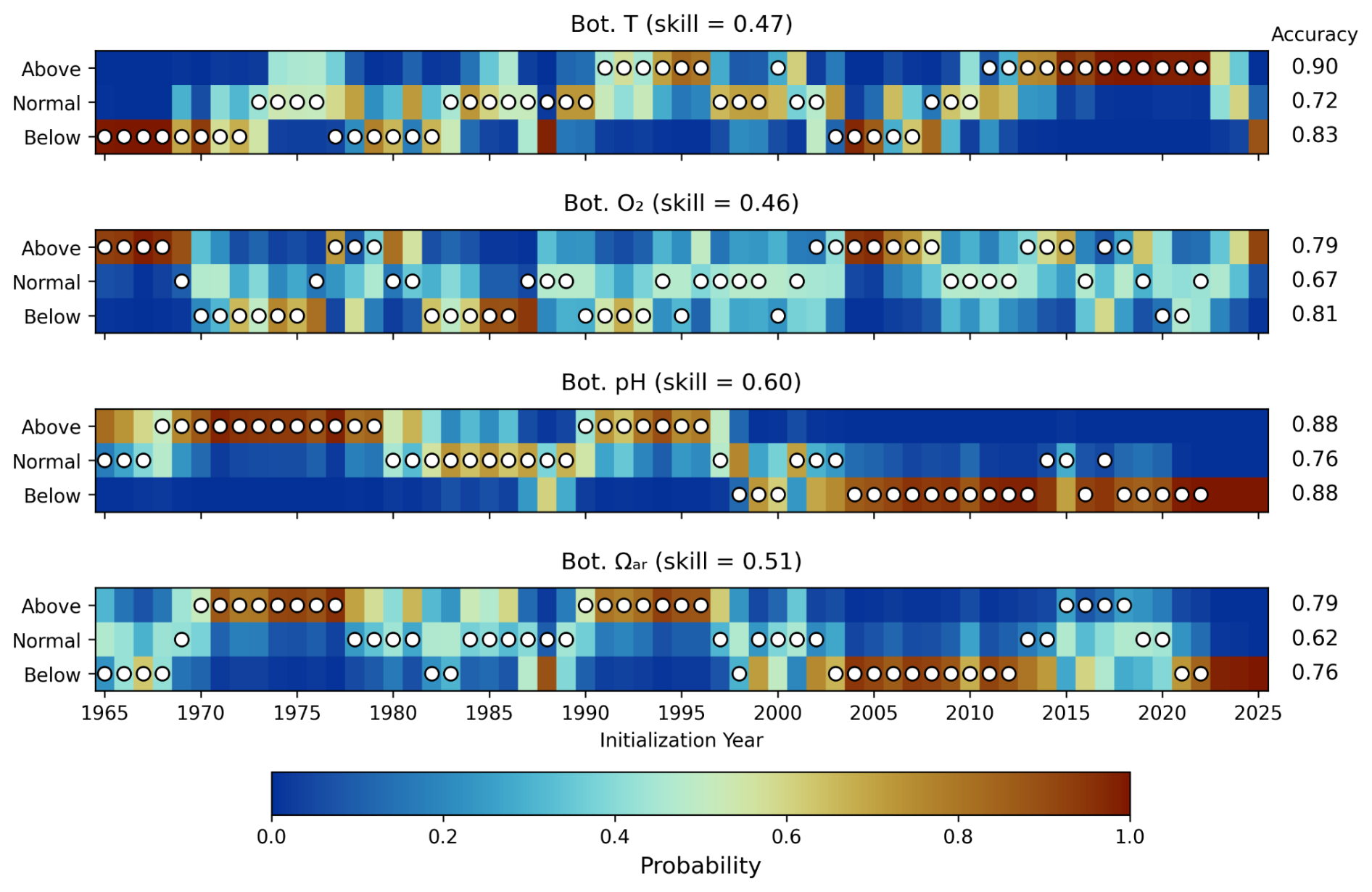
Figure 7 Probabilistic predictions for the GOM. Probability of the predicted lead 1–3 year mean anomalies (with respect to the 1994–2023 mean) of (a) bottom temperature, (b) bottom O₂, (c) bottom pH and (d) bottom Ω_ar from the regional downscaled decadal prediction model (NWA12_HIND). The corresponding classifications of the reference anomalies are shown as white circles from the regional downscaled simulation (NWA12_EN4_NUDG). The tercile boundaries are calculated separately for the predictions and reference/observations. The x axis shows the initialization year and the 2025 forecast. The forecast accuracy, (True Positives + True Negatives)/Total forecasts, for each tercile is shown on the right. A random forecast that randomly picks one tercile as most likely for each forecast has an accuracy of 0.56 and the accuracy of a consistently negative (counter) prediction is 0.67. The forecast skill compared to persistence is given in the subtitle of each panel.

The RPSS for all quantities is >0, indicating the model has some capacity to anticipate changes (i.e., probabilistic skill beyond the persistence forecast, see Sect. 2). Oxygen has slightly lower skill (RPSS 0.46, accuracy 0.67–0.81) compared to bottom temperature (RPSS 0.47, accuracy 0.72–0.90), reflecting both the weak predictable climate change signals and the influence of less predictable atmospheric variability. Similarly, predictions for bottom pH, which has a very strong predictable climate change signal, have higher skill (RPSS 0.6, accuracy 0.76–0.88) than Ω_ar (RPSS 0.51, accuracy 0.62–0.79).

The high accuracy of prediction for bottom temperature, O₂, pH and Ω_ar likely reflects both methodological and mechanistic factors. The bottom temperature, O₂, pH and Ω_ar are validated against the same regional downscaled simulation from which initial conditions were derived (see Sect. 2). While this simulation recreates observed O₂ patterns and covariances with well-constrained physical properties to the extent that they have been observed (Figs. 2, 3 and S7), it should be viewed as an upper limit for prediction skill. Additional autonomous biogeochemical observing platforms capable of observing shelf environments may help address this limitation in the future (Henson, 2014; Chai et al., 2020).

Looking ahead over the next three years (2025–2027), we forecast below-normal bottom temperatures with high confidence (88.3 % probability), supported by 93.3 % retrospective accuracy when issuing similar high confidence forecasts ($\mathrm{14}/\mathrm{15}$ hits). We also predict above-normal bottom O₂ levels with high confidence (92.0 % probability), with an 85.7 % retrospective accuracy at comparable confidence levels ($\mathrm{6}/\mathrm{7}$ hits). Additionally, we forecast with very high confidence (>99 % probability) both below-normal bottom pH and below-normal Ω_ar conditions, both of which are supported by perfect retrospective accuracy when issuing very high confidence forecasts, albeit with limited sample size ($\mathrm{9}/\mathrm{9}$ hits and $\mathrm{1}/\mathrm{1}$ hit respectively). While these forecasts represent our best estimate, both the confidence levels and the underlying sample sizes should be considered when making decisions based on these predictions, particularly for the forecasts where limited similarly confident historical forecasts constrain our ability to fully validate forecast skill. Nevertheless, the dynamically consistent physical and biogeochemical forecasts provide compelling evidence that the ongoing watermass reorganization will continue to influence bottom water conditions through the 2025–2027 period.

4 Discussion: towards the future of fisheries management

Future projections indicate the entire GOM will experience suboptimal aragonite saturation for most of the year by 2050 under high emissions scenarios (Siedlecki et al., 2021). The region's demonstrated sensitivity to water mass-driven alkalinity variations makes it particularly vulnerable to rapid acidification once rising CO₂ exceeds the buffering ability of the projected increased Gulf Stream water, potentially triggering swift transitions to persistently corrosive conditions that could impact economically vital shellfish industries (Ekstrom et al., 2015). Although the recent transition from a decade of warm water influence to emerging cold water conditions across portions of the Northeast US Continental Shelf, including the deep GOM (Record et al., 2024), may buy time for fisheries to adapt to the projected long-term warming trend, it also may accelerate or alter the projected biogeochemical shifts.

We assessed the decadal prediction skill for the Gulf of Maine, a semi-enclosed body of water on the Northeast US Continental Shelf. While the patterns of prediction skill that emerged from the interplay of climate change signals and variability were unique to each quantity and the Gulf of Maine, other coastal regions are subject to similar oceanic and atmospheric forcing (Shearman and Lentz, 2010) and may present opportunities for bottom-habitat prediction. The ubiquity of sea surface temperature prediction skill in coastal systems at seasonal and decadal scales provides grounds for optimism (Stock et al., 2015; Tommasi et al., 2017b). The methodologies employed herein, while computationally intensive, provide a robust means to diagnose the origins of predictive skill and attach probabilities critical to making forecast information actionable for management applications.

More frequent and extensive observations of the ocean, including deep ocean biogeochemistry, are essential for increasing confidence in the accuracy of the forecasts and providing confirmation of predicted changes (Capotondi et al., 2019). Observations are especially important for verifying interannual to decadal scale ocean predictions, where long time series are necessary to verify that the predictions have more skill than simple forecasts of the forced signal or autocorrelated noise. Here, given the scarcity of past deep alongshelf biogeochemical observations, we utilized a numerical model as the reference for forecast verification. This downscaled simulation was validated using the best available observations (Figs. 2, S1–S3, S6 and S7). Consequently, the reported skill represents potential skill and may be an overestimation. However, the model successfully simulated observed variability in bottom temperature and salinity and captured the expected covariance between these two variables and the bottom biogeochemistry. Koul et al. (2024) also demonstrated forecast skill for surface temperature when compared against actual observations. Furthermore, the model is likely accurate in predicting much of the forced component of skill, which is driven by steadily increasing greenhouse gas concentrations and resulting impacts on ocean warming and chemistry.

Our forecasts of continued cooling alongside below-normal bottom pH, Ω_ar and above-normal bottom O₂ levels through 2027 reveal the substantial biogeochemical fingerprint of this water mass transition and potentially offer stakeholders lead time to anticipate ecosystem shifts. Skillful forecasts on these multi-year timescales can meet critical needs of fishers, managers, conservationists, and other stakeholders (Link et al., 2023; Saba et al., 2023). The framework developed here, consisting of a computationally efficient regional model that downscales regularly updated global predictions, is well positioned to meet these needs and is intended to be transitioned towards operational use through NOAA's Changing Ecosystems and Fisheries Initiative. Recognizing that marine resource management is a wicked problem (Jentoft and Chuenpagdee, 2009; Rittel and Webber, 1973), however, careful application-specific analyses of the potential costs, benefits, and tradeoffs of using these forecasts for decision-making will be necessary.