Local dissipation ratio of internal tides at key topographic features in the South China Sea

The local dissipation ratio of internal tides, q^*, is a critical parameter in tidal mixing parameterizations. However, the conventionally adopted constant value of 0.3 in large-scale ocean models neglects its significant spatiotemporal variability. Based on the MITgcm LLC4320 simulation, the internal tidal energy budgets at the Luzon Strait (a source region, LS) and the Nansha Islands (a sink region, Nansha) in the South China Sea (SCS) are analyzed. Results indicate that the barotropic-to-baroclinic energy conversion in the LS reaches approximately 45 GW, with semidiurnal constituents accounting for roughly 60 %, due to the resonance over the double-ridge topography. The q^* value of the total internal tide in the LS fluctuates between 0.3 and 0.7, primarily modulated by the local dissipation of modes 3–5. Local internal tide generation around the Nansha Islands is less than 1.5 GW; however, this region experiences significant convergence of internal tidal energy flux, so that the q^* value of the total internal tide is generally larger than 1 and occasionally exceeds 2.5. Modal analysis confirms that the intensified dissipation over the Nansha Islands originates predominantly from topographic scattering and breaking of mode-1 internal tides from the far field. Parameterizations for q^* are developed based on both physical factors and data-driven algorithms, both of which successfully capture the macroscopic clustering of q^*. In the LS, q^* is modulated by near-field factors such as the barotropic tidal forcing and the local dissipation of modes 3–5. Conversely, q^* around the Nansha Islands is primarily contributed by mode-1 internal tidal energy coming from the far field, highlighting the joint modulation of local extreme dissipation by far-field beam interference and nonlinear topographic scattering.

1 Introduction

Diapycnal mixing in the ocean is a key dynamical process that maintains the global ocean stratification, shapes the meridional overturning circulation, and regulates the transport of heat, energy, and nutrients (Munk and Wunsch, 1998; Wunsch and Ferrari, 2004). In the deep ocean, the interaction of barotropic tides with rough topography generates internal tides, which are widely regarded as the primary mechanical energy source furnishing deep-ocean mixing (Egbert and Ray, 2000; Garrett and Kunze, 2007; Ferrari and Wunsch, 2009). It is estimated that approximately 1 TW of barotropic tidal energy is converted into internal tides, accounting for roughly half of the total energy required to maintain global abyssal mixing (Egbert and Ray, 2003; Nycander, 2005). However, after generation, internal tidal energy undergoes radiation, loss of phase coherence, topographic scattering, and irreversible dissipation, each playing a distinct role in the internal tide energy budget. Radiation transports internal tidal energy away from the generation region through the baroclinic energy flux (St. Laurent and Garrett, 2002). Loss of phase coherence reduces the stationary (i.e., harmonically detectable) component without necessarily reducing the total internal tidal energy. Topographic scattering redistributes incident internal tidal energy across different propagation directions and vertical modes rather than dissipating it directly (i.e., without net energy loss); however, by transferring energy to higher, more dissipative modes, it indirectly promotes subsequent wave breaking (MacKinnon et al., 2017). Irreversible dissipation removes internal tidal energy from the internal wave field as energy cascades nonlinearly to progressively smaller scales, ultimately triggering wave breaking and turbulence, which drive diapycnal mixing (Waterhouse et al., 2014). Usually, these processes are intertwined. For instance, Alford et al. (2019) estimated the spatial attenuation of the mode-1 M₂ internal tide energy flux, which consists of both a stationary component detected by multisatellite altimetry and a nonstationary component corrected using an eddy-resolving tidal model. Across the North Pacific, the total fluxes yield e-folding scales of approximately 750–3000 km. This apparent decrease in the total flux includes actual loss of mode-1 energy, through irreversible dissipation or scattering to higher modes, as well as loss of phase coherence (i.e., reduced stationarity). Therefore, accurately quantifying the spatiotemporal distribution of the local internal tidal dissipation is crucial for improving the performance of ocean circulation and climate models (Melet et al., 2016; de Lavergne et al., 2020).

In state-of-the-art climate-scale ocean models, the mixing induced by internal tidal breaking cannot be explicitly resolved due to limitations in grid resolution and must therefore be parameterized (Jayne, 2009). The local dissipation efficiency, q, is a decisive dimensionless parameter defined as the fraction of locally generated internal tidal energy that dissipates near the generation site, with the remainder radiating away as low-mode internal tides; thus, q is restricted between 0 and 1; it directly modulates the spatial distribution of internal tidal energy (St. Laurent et al., 2002). In an internal tide source region, a lower q indicates that a larger fraction of the locally generated internal tidal energy propagates toward the far field as low-mode internal tides; a higher q indicates stronger near-field dissipation, leading to enhanced local mixing (Klymak et al., 2011; Vic et al., 2019). For a long time, to simplify calculations, ocean circulation models have typically prescribed q as a globally uniform constant of 0.3 (Simmons et al., 2004; Saenko and Merryfield, 2005). However, recent studies have demonstrated significant spatial heterogeneity in q. Lefauve et al. (2015) noted its topographic dependence, and Vic et al. (2019) further elucidated that q is regulated by the vertical modal structure of internal tides via a global semi-analytical model. Over small-scale rough topography, high-mode internal tides are predominantly generated, yielding high q values (>0.8); whereas over large-scale steep topography, low-mode internal tides prevail, leading to low q values (< 0.4). Ignoring the spatiotemporal variability of q causes an order-of-magnitude miscalculation of the mechanical energy supplying internal tidal mixing, thereby significantly reducing the model's capacity to simulate the evolution of water masses and the intensity of global meridional overturning circulation (Cimoli et al., 2019).

As the largest marginal sea in the western Pacific and one of the most well-known hotspots for internal tides, the South China Sea (SCS) is an ideal study area for quantifying internal tidal energy budgets and exploring the spatiotemporal evolution of the dissipation parameter q due to its complex dynamical environment. The SCS not only encompasses the Luzon Strait (LS), a globally recognized strong internal tidal source region (Niwa and Hibiya, 2004; Jan et al., 2007), but also contains complex topographies such as the Nansha Islands (Nansha) and the Dongsha Islands, both located within or adjacent to the basin, which serve as key sink regions for internal tidal energy. Internal tidal energy budget analysis by Wang et al. (2016) revealed that the total local dissipation accounts for 38% of the local conversion in the LS during summer, whereas in the broader SCS it is 267 % of the local conversion. Tian et al. (2025) reported that during summer about 24% of the baroclinic tidal energy generated in the LS is dissipated locally, and in the broader SCS the total local dissipation is 203 % of the local conversion. When low-mode internal tides propagate over rough topography far from the source regions, topographic scattering effects promote the energy transfer to high modes, thereby enhancing the dissipation there (Klymak et al., 2010). Therefore, we define the local dissipation ratio of internal tides, q^*, as the area-integrated total local dissipation inferred from the baroclinic energy budget divided by the area-integrated barotropic-to-baroclinic conversion. q^* is normalized by the same local conversion as the conventional q, but its numerator may be furnished by both local conversion and the convergence of internal tidal energy from the far field. Consequently, in source regions (such as the Luzon Strait) q^* has the same meaning as q and normally ranges from 0 to 1, whereas in sink regions (such as the Nansha Islands) it may exceed 1.

Although the generation and propagation of internal tides in the SCS have been extensively explored in previous studies (Zhao et al., 2010; Tian et al., 2025), research on q and its parameterizations remains significantly inadequate. First, existing studies mostly focus on estimating the spatial distribution of q globally and its magnitude in internal tide generation regions. There is a lack of analysis of the temporal variation of q^* and of systematic comparison of the differences in q^* between source and sink regions for internal tidal energy. Second, although it is theoretically established that q depends on the internal tidal modal structure and may be related to topographic gradients and the shear intensity of background flow fields (Polzin, 2004; Dunphy and Lamb, 2014), most global ocean circulation models still use empirical constants to set q, neglecting its spatiotemporal variability. Wang and Legg (2023, 2025) examined how baroclinic eddy shear affects internal tide refraction, modal energy transfer, and dissipation, and showed that the shear current associated with strong baroclinic eddies can transfer part of the incident mode-1 internal tide energy into higher modes and trap these high modes within the eddies, thereby making the eddies hotspots for internal tide dissipation. Therefore, exploring the spatiotemporal variations of q^* under different dynamical environments and developing physically consistent parameterizations are essential for accurately simulating internal tidal mixing.

In this study, we intend to diagnose the internal tidal energy budgets, quantify the temporal variations and regional differences of the local dissipation ratio q^*, and establish parameterizations of q^* for two representative internal tidal regions, a source region (LS) and a sink region (Nansha Islands) in the SCS. In Sect. 2, we introduce the utilized data from the MITgcm LLC4320 simulation output, the methods for vertical modal decomposition and internal tidal energy budget analysis, and the eXtreme Gradient Boosting (XGBoost) model employed to predict q^*. Section 3 presents the results of internal tidal energy budgets and q^* in the LS and the Nansha Islands, respectively. Specifically, the tidal energy budgets and q^* are analyzed for each vertical mode separately. Then, the performance of the q^* parameterizations based on both the physical-based empirical formulation and the XGBoost model is demonstrated. Finally, our results are summarized in Sect. 4.

2 Data and methods

2.1 Data

The data used in this study are the LLC4320 simulation outputs from the Massachusetts Institute of Technology general circulation model (MITgcm), which solves the Navier-Stokes equations under the hydrostatic and Boussinesq approximations. The model is forced by the complete luni-solar tidal potential including 16 principal tidal constituents (such as M₂, S₂, K₁, and O₁) and by the 6-hourly atmospheric reanalysis dataset provided by the European Centre for Medium Range Weather Forecasts (ECMWF) (Marshall et al., 1997; Arbic et al., 2018). An Arakawa-C grid mesh is used in the simulation with a horizontal resolution of 1/48° (approximately 2 km in the SCS). In the vertical, the model has 90 z-coordinate levels, with layer thickness increasing from 1 m at the surface to around 480 m near the seabed. The hourly output of three-dimensional velocity, potential temperature, salinity, and sea surface height from 13 September 2011 to 15 November 2012 is used, with specific focus on two key topographic regions, the LS and the Nansha Islands (Fig. 1). The Luzon Strait domain is defined to encompass the Hengchun Ridge, the Lanyu Ridge, and the inter-ridge trough, which collectively constitute the double-ridge where intense internal tides are generated (Buijsman et al., 2014; Tian et al., 2025; Wang et al., 2016). The Nansha Islands domain is selected to encompass the dominant topographic features (islands and reefs), which are located in the propagation paths of internal tides coming from the LS (Tian et al., 2025; Xu et al., 2016). The interaction of the incoming internal tides with the rough islands and reefs promotes energy transfer to higher modes and hence enhances local dissipation (Vic et al., 2019).

2.2 Methods

The subtidal fields ($\stackrel{\mathrm{‾}}{\mathit{u}}$ and $\stackrel{\mathrm{‾}}{\mathit{\rho }}$) are obtained by applying a 3 d moving average to the total fields, and the perturbation fields (u^′, ρ^′) are obtained by subtracting the subtidal fields from the total ones. The barotropic velocity ${\mathit{u}}_{\mathrm{bt}}^{\prime }=(u_{\mathrm{bt}}^{\prime },v_{\mathrm{bt}}^{\prime })$ is defined as the depth-averaged velocity, and the baroclinic velocity is calculated as ${\mathit{u}}_{\mathrm{bc}}^{\prime }={\mathit{u}}^{\prime }-{\mathit{u}}_{\mathrm{bt}}^{\prime }$. A bandpass filter is then applied to extract the diurnal (D1, 0.90–1.10 cpd) and semidiurnal (D2, 1.87–2.10 cpd) tidal constituents. When diagnosing the internal tidal energy budgets and q^* for individual vertical modes, a vertical modal decomposition method is employed. The modal structure function ϕ_n(z) can be obtained by solving the Sturm–Liouville equation (Gill, 1982):

$$\begin{array}{}\text{(1)}& {\displaystyle \frac{{\mathrm{d}}^{\mathrm{2}}{\mathit{\varphi }}_n\left(z\right)}{\mathrm{d}{z}^{\mathrm{2}}}}+{\displaystyle \frac{N^{\mathrm{2}}\left(z\right)}{c_n^{\mathrm{2}}}}{\mathit{\varphi }}_n\left(z\right)=\mathrm{0},\end{array}$$

where boundary conditions are given as ${\mathit{\varphi }}_n\left(\mathrm{0}\right)={\mathit{\varphi }}_n(-H)=\mathrm{0}$, and H is the water depth. Here, N(z) is the buoyancy frequency, c_n is the eigenspeed, and n is the mode number. Due to the orthogonality of the modes, the baroclinic velocity ${\mathit{u}}_{\mathrm{bc}}^{\prime }$ and the pressure perturbation p^′ can be expressed as ${\mathit{u}}_{\mathrm{bc}}^{\prime }(z,t)=\sum _{n=\mathrm{1}}^N{\mathit{U}}_n\left(t\right){\mathit{\phi }}_n\left(z\right)$, $p^{\prime }(z,t)=\sum _{n=\mathrm{1}}^N{P}_n\left(t\right){\mathit{\phi }}_n\left(z\right)$, where ${\mathit{\phi }}_n\left(z\right)=\mathrm{d}{\mathit{\varphi }}_n\left(z\right)/\mathrm{d}z$ is the vertical structure for horizontal velocity and pressure, U_n(t) and P_n(t) are the coefficients of individual modes, and N=5 is the total number of modes used in this study. Taking January and August 2012 as representative cases, in the LS and the Nansha Islands, modes 1–5 account for 85 % and 89 % of the total baroclinic kinetic energy, 87 % and 99 % of the diurnal baroclinic kinetic energy, and more than 98 % of the semidiurnal baroclinic kinetic energy, respectively. Modes 1–5 capture the dominant part of total baroclinic kinetic energy, while the remaining fraction (mode 6 and above) does not exceed 15 % of the total baroclinic kinetic energy, although these unretained higher modes may still contribute less to local dissipation of internal tides over rough topography (Vic et al., 2019).

To evaluate the generation and dissipation of internal tidal energy, the depth-integrated baroclinic energy equation is used here. After tidal-period averaging and neglecting the tendency and advection terms, the energy equation reduces to (Niwa and Hibiya, 2004):

$$\begin{array}{}\text{(2)}& 〈{\mathrm{DIS}}_{\mathrm{bc}}〉=\langle \mathrm{Conv}\rangle -〈{\mathrm{\nabla }}_h\cdot \mathit{F}〉,\end{array}$$

where 〈⋅〉 denotes the tidal-period mean. Conv is the depth-integrated barotropic-to-baroclinic energy conversion, indicating the local internal tide generation, which can be calculated as:

$$\begin{array}{}\text{(3)}& \mathrm{Conv}=\underset{-H}{\overset{\mathit{\eta }}{\int }}{\mathit{\rho }}^{\prime }g{w}_{\mathrm{bt}}^{\prime }\mathrm{d}z,\end{array}$$

where η is the sea level displacement, and $w_{\mathrm{bt}}^{\prime }$ is the vertical velocity induced by the barotropic tides. This vertical velocity $w_{\mathrm{bt}}^{\prime }$ is given by $w_{\mathrm{bt}}^{\prime }=u_{\mathrm{bt}}^{\prime }\left(\mathit{\sigma }\frac{\partial D}{\partial x}+\frac{\partial \mathit{\eta }}{\partial x}\right)+v_{\mathrm{bt}}^{\prime }\left(\mathit{\sigma }\frac{\partial D}{\partial y}+\frac{\partial \mathit{\eta }}{\partial y}\right)+(\mathit{\sigma }+\mathrm{1})\frac{\partial \mathit{\eta }}{\partial t}$ (Mellor, 2004), where D is the total water depth, $D=H+\mathit{\eta }$, and $\mathit{\sigma }=(z-\mathit{\eta })/D$. A positive Conv denotes conversion from barotropic to baroclinic energy, that is, local internal tide generation, whereas a negative Conv denotes the reverse (baroclinic-to-barotropic) conversion. F is the depth-integrated baroclinic energy flux, and ∇_h⋅F is the horizontal divergence of F. A positive ∇_h⋅F indicates outward propagation of internal tidal energy from the local region; a negative ∇_h⋅F indicates convergence of energy flux from the far field. F is given as:

$$\begin{array}{}\text{(4)}& \mathit{F}=\underset{-H}{\overset{\mathit{\eta }}{\int }}{\mathit{u}}_{\mathrm{bc}}^{\prime }{p}^{\prime }\mathrm{d}z,\end{array}$$

where p^′ is calculated as $p^{\prime }(z,t)=-\frac{\mathrm{1}}{H}\underset{-H}{\overset{\mathit{\eta }}{\int }}\underset{z}{\overset{\mathit{\eta }}{\int }}g{\mathit{\rho }}^{\prime }(\widehat{z},t)\mathrm{d}\widehat{z}\mathrm{d}z+\underset{z}{\overset{\mathit{\eta }}{\int }}g{\mathit{\rho }}^{\prime }(\widehat{z},t)\mathrm{d}\widehat{z}$. DIS_bc is the depth-integrated local dissipated internal tidal energy, inferred as the residual of the simplified depth-integrated baroclinic energy equation (Eq. 2) rather than a diagnosed dissipation from the model. A positive DIS_bc denotes net dissipation of baroclinic energy inferred from the energy budget; a negative DIS_bc denotes a net gain of baroclinic energy. In some studies, the dissipation can also be diagnosed from the simulation using the velocity gradients and the horizontal and vertical eddy viscosity coefficients (Nikurashin and Legg, 2011). However, in the LLC4320 simulation, horizontal eddy viscosity is determined internally by a parameterization scheme and is not provided as an output; therefore, we cannot exactly diagnose dissipation from the model output. There exist both connections and differences between the inferred dissipation and the diagnosed dissipation: the former not only includes the latter (i.e., explicit numerical dissipation), but also covers other physical processes such as bottom friction dissipation. Fortunately, their quantitative discrepancy is not critical. For example, assuming a constant horizontal eddy viscosity, Fan et al. (2024) compared the diagnosed dissipation from the LLC4320 simulation with the inferred dissipation from the energy budget equation. They found that these two dissipation fields exhibit comparable magnitudes and broadly consistent spatial patterns across the northern SCS, despite localized discrepancies attributed to the constant horizontal eddy viscosity assumption.

The local internal tidal dissipation ratio, q^*, is defined as the ratio of the area-integrated DIS_bc to Conv, i.e., $q^{*}=\underset{s}{\int }\mathrm{d}s\left({\mathrm{DIS}}_{\mathrm{bc}}\right)/\underset{s}{\int }\mathrm{d}s\left(\mathrm{Conv}\right)$. Here, the spatial integration domain s corresponds to the red-boxed regions shown in Fig. 1. Based on the above calculations, the internal tidal energy budgets and q^* for different tidal components and different vertical modes can be estimated. In this way, q^* is not necessarily restricted between 0 and 1. $q^{*}>\mathrm{1}$ occurs when the area-integrated divergence of the baroclinic energy flux is negative, indicating a convergence of far-field internal tidal energy. In this case, the inferred local dissipation exceeds the barotropic-to-baroclinic energy conversion. For individual vertical modes, $q^{*}<\mathrm{0}$ occurs when the area-integrated divergence of the baroclinic energy flux of this mode exceeds its local barotropic-to-baroclinic energy conversion, yielding a negative inferred dissipation. The divergence of the baroclinic energy flux is furnished by both the local conversion and the net energy transfer from other vertical modes, and may therefore exceed the local barotropic-to-baroclinic energy conversion. Incomplete months (September 2011 and November 2012) are excluded when computing the monthly mean values of q^*. January and August 2012 are selected as winter and summer months in the simulated year, respectively.

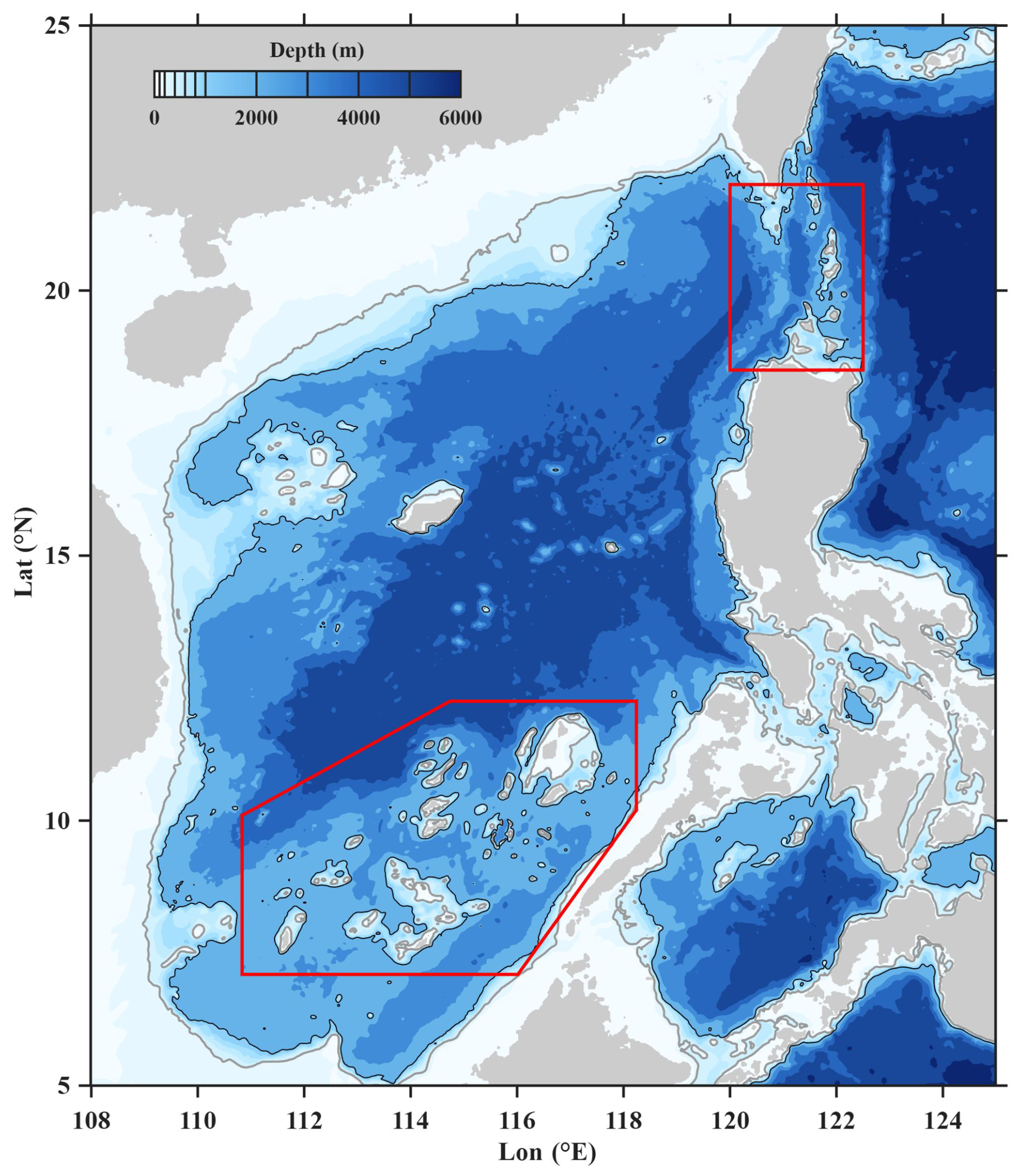
Figure 1 Topography of the SCS. Gray and black contours represent the 200 and 1000 m isobaths, respectively. Red boxes represent the key topographic regions, including the LS and the Nansha Islands.

To develop a more robust parameterization of q^*, this study not only adopts a physical-based empirical formulation but also uses the XGBoost model jointly, which can make up for the limitations of traditional physical-based empirical formula in complex dynamic environments. The model inputs include 6 physical features, namely the internal tidal shear averaged within the bottommost 500 m, stratification, barotropic tidal kinetic energy, mode-1 internal tidal energy, the proportion of mode-1 internal tidal energy in the total internal tidal energy, and the mode-1 internal tidal group velocity. The data from the LS and the Nansha Islands are sequentially combined into a training set, a validation set, and a test set with proportions of 70 %, 15 %, and 15 %, respectively. Considering the differences in the physical processes governing q^* between the internal tidal source regions and sink regions, this study constructs two separate models, one for the LS and one for the Nansha Islands. The Mean Absolute Error (MAE) is adopted as the objective loss function, i.e., $\mathrm{MAE}=\frac{\mathrm{1}}{n}\sum _{i=\mathrm{1}}^n\left|{\widehat{y}}_i-y_i\right|$, where y_i and ${\widehat{y}}_i$ denote the actual and predicted values, respectively, and n is the number of samples. An early stopping iteration setting of 500 rounds and 800 rounds are applied for models of the LS and Nansha Islands, respectively.

3 Results

3.1 Local dissipation ratio of internal tides in the LS

The internal tidal energy budget in the LS is characterized by intense generation, strong outward radiation, and relatively low q^*. The barotropic-to-baroclinic conversion in the LS ranges from 40 to 50 GW, of which 15–25 GW radiates out of the LS (Fig. 2g), yielding a q^* value of approximately 0.5 (Fig. 2h). The semidiurnal wavelength better matches the alignment of the double ridges in the LS, resulting in a larger semidiurnal tide generation (20–30 GW) than diurnal tide generation (10–25 GW) (Fig. 2g). The semidiurnal dissipation (10–20 GW) and q^* values (0.6–0.8) are also higher than those of the diurnal tide, whose dissipation ranges from 1 to 10 GW and q^* from 0.1 to 0.6 (Fig. 2g and h). The semidiurnal conversion, dissipation, and q^* are larger in summer than in winter (Fig. 2g and h). The diurnal q^* reaches minima of 0.1 and 0.3 in February–March and June–July, respectively (Fig. 2h).

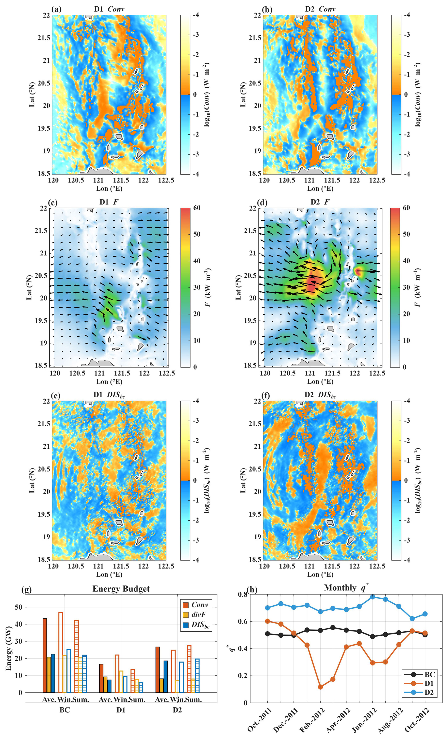
Figure 2 (a–f) Spatial distributions of the diurnal and semidiurnal internal tidal energy budget terms in the LS during summer. 〈Conv〉 is the tidal-period mean depth-integrated barotropic-to-baroclinic energy conversion, 〈F〉 is the tidal-period mean depth-integrated internal tidal energy flux, and 〈DIS_bc〉 is the tidal-period mean depth-integrated local internal tidal dissipation. (g) Bar chart of the budget terms. 〈divF〉 is the tidal-period mean divergence of the depth-integrated internal tidal energy flux. “Ave.”, “Win.”, and “Sum.” stand for the annual-, winter-, and summer-mean values, respectively. BC, D1, and D2 represent the total internal tide, diurnal tide, and semidiurnal tide, respectively. (h) Time series of the monthly-mean local internal tidal dissipation ratio, q^*. In (a), (b), (e) and (f), the units for Conv and DIS_bc are W m⁻², with orange (blue) representing positive (negative) values. In (c) and (d), the unit for F is kW m⁻¹, with colors representing magnitude and arrows indicating direction. In (g), the units for Conv, divF, and DIS_bc are GW.

The summer spatial distributions demonstrate that internal tide generation and dissipation are concentrated over and around the double ridges (Fig. 2a, b, e and f). Substantial internal tidal energy propagates westward and northwestward from the western ridge into the SCS (Fig. 2c and d). The semidiurnal component plays a dominant role in the internal tide generation and dissipation (Fig. 2a, b, e and g). The q^* values ranging from 0.49 to 0.57 in the LS are comparable to those in other representative internal tide generation regions; for example, You et al. (2023) estimated a value of about 0.58 for the M₂ internal tide at the Aleutian Ridge, suggesting that q^* values in submarine ridges serving as internal tide source regions share a similar magnitude.

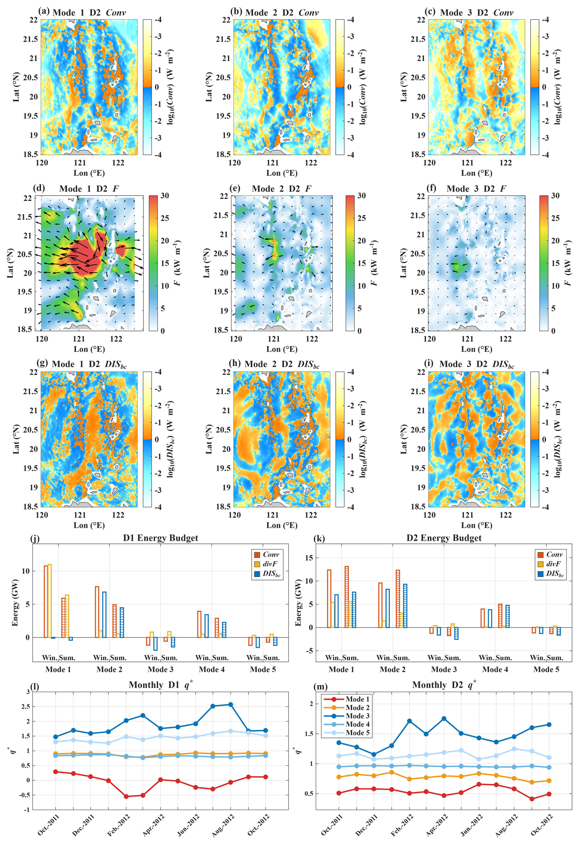
Figure 3 (a–i) Spatial distributions of the semidiurnal internal tidal energy budget terms for modes 1–3 in the LS during summer. (j, k) Bar charts of the energy budget terms for modes 1–5, and (l, m) time series of monthly-mean q^* for modes 1–5 for diurnal (D1) and semidiurnal (D2) tides, respectively. “Win.” and “Sum.” stand for winter and summer, respectively. In (a)–(c) and (g)–(i), the units for Conv and DIS_bc are W m⁻², with orange (blue) indicating positive (negative) values. In (d)–(f), the unit for F is kW m⁻¹, with colors indicating magnitude and arrows indicating direction. In (j) and (k), the units for Conv, divF, and DIS_bc are GW. In (l) and (m), monthly mean values of q^* outside the displayed y axis ranges are not shown for clarity.

The internal tidal energy budgets and q^* in the LS exhibit differences among individual tidal components and vertical modes. Both diurnal and semidiurnal internal tide generation are dominated by modes 1–2, with mode 1 accounting for roughly 50 % of the total generation and exhibiting an energy flux divergence greater than those of other modes (Fig. 3j and k). The divergence of diurnal mode-1 energy flux is even larger in magnitude than the local generation (Fig. 3j), resulting in negative q^* values (Fig. 3l), implying that the internal tidal energy generated in the LS radiates outward as low-mode internal tides intensively. Tian et al. (2025) indicated that the diurnal tide has a larger decay scale than the semidiurnal tide, which favors more outward radiation of the diurnal tide as mode 1. By contrast, although the semidiurnal energy budget is also dominated by modes 1–2, the proportion of mode-1 energy flux divergence is relatively smaller, and its difference between January and August 2012 is weaker than that of the diurnal tide (Fig. 3j and k). Regarding local dissipation, q^* for modes 3–5 of both the diurnal and semidiurnal components ranges from 0.8 to 2.7, significantly larger than that of modes 1–2 (<0.8) (Fig. 3l and m).

The strongly positive generation regions for modes 1–2 internal tides are concentrated at the crests of the double ridges, whereas the high-generation regions for mode 3 are distributed along the ridge flanks (Fig. 3a–c). The energy budget of the mode-1 internal tide is characterized by substantial energy propagating northwestward and westward into the SCS, as well as eastward into the Pacific Ocean (Fig. 3d). The majority of the mode-1 semidiurnal energy flux enters the SCS, with peak values reaching 25 kW m⁻¹ (Fig. 3d). Local dissipation gradually weakens and becomes spatially dispersed with increasing mode number (Fig. 3g–i). At the Mid-Atlantic Ridge and the Hawaiian Ridge, Vic et al. (2018) indicated that a dominant proportion of mode-1 internal tide generation facilitates the outward radiation of substantial energy as low-mode internal tides, yielding small values of the dissipation ratio. This result confirms the robust far-field radiation capacity of internal tides and the smaller q^* values of mode 1 relative to those of higher modes in the LS.

3.2 Local dissipation ratio of internal tides in the Nansha Islands

In contrast to the LS, the internal tidal energy budget of the Nansha Islands is characterized by low local generation, strong energy convergence, and a high value of q^*. The local generation of internal tides in the Nansha Islands is weak, fluctuating between 0.6 and 1.3 GW, whereas the incoming internal tidal energy flux can reach 1.5 GW (Fig. 4g). This energy budget (dominated by far-field input) directly elevates q^* values to 1.0–3.0 (Fig. 4h). Both the local generation and the energy flux of the diurnal tide dominate those of the semidiurnal tide (Fig. 4g), maintaining the q^* of the diurnal tide in the range of 1.5–3.0, which is larger than the q^* of the semidiurnal tide varying between 1.0 and 2.0 (Fig. 4h).

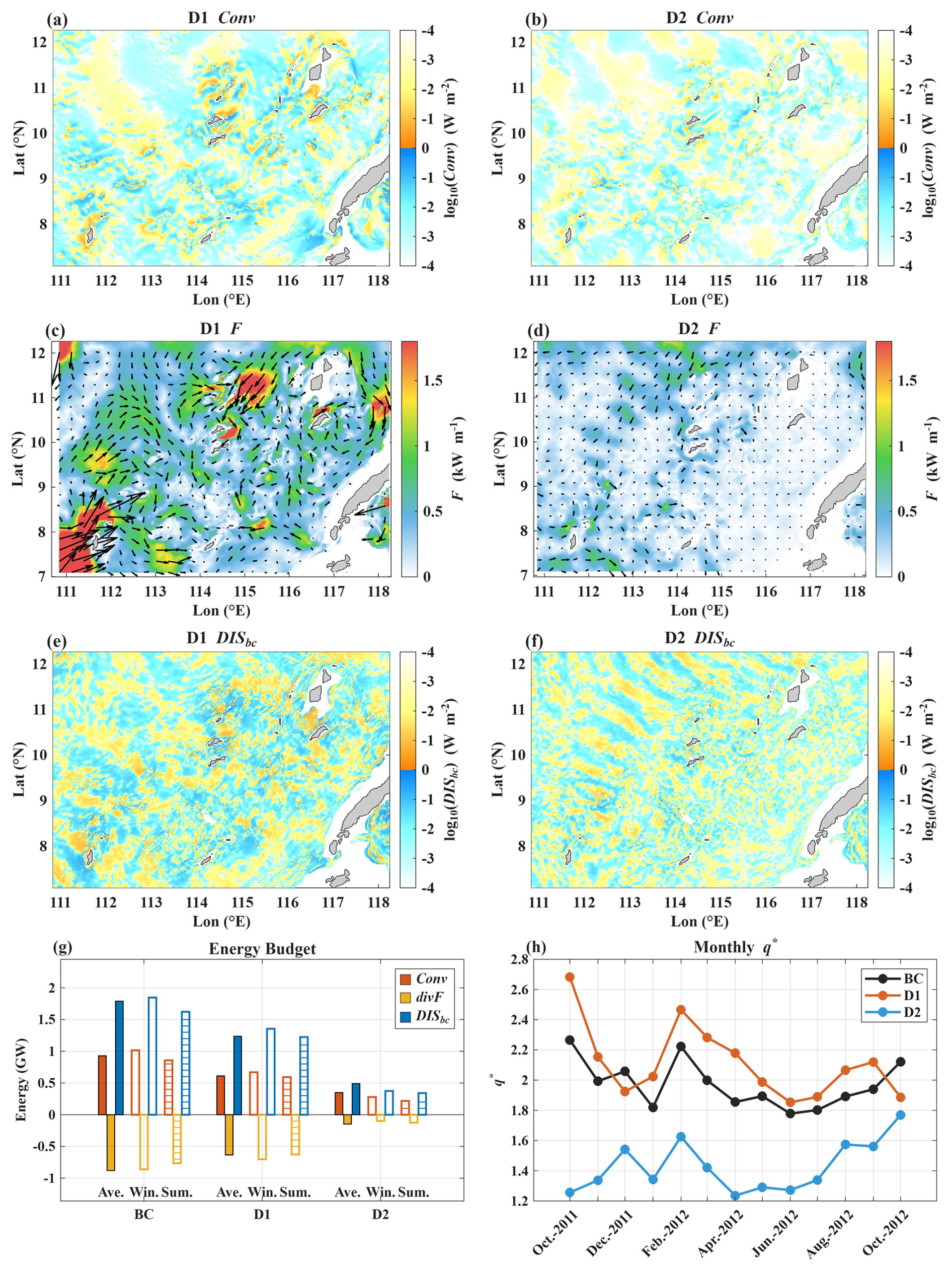
Figure 4 Same as Fig. 2, but for the Nansha Islands.

Both the generation and local dissipation of internal tides in the Nansha Islands exhibit a scattered patchy pattern, with high values concentrated around reefs (Fig. 4a, b, e and f). All the energy budget terms of the diurnal tide are larger than those of the semidiurnal tide (Fig. 4a–f), with a significant incoming diurnal energy flux of approximately 1.5 kW m⁻¹ at the southwestern and northern boundaries of the Nansha Islands (Fig. 4c). Kelly et al. (2013) estimated that at continental margins, incident mode-1 internal tidal energy is partitioned among reflection, transmission, and scattering to higher modes. Lahaye et al. (2020) demonstrated that incident low-mode internal tides can be scattered to higher modes through interactions with steep topography. Subsequently, high-mode internal tides are susceptible to breaking near their generation sites (Siyanbola et al., 2024). Modal scattering redistributes internal tidal energy rather than dissipating it; the breaking of the scattered high modes constitutes the irreversible dissipation. It is therefore reasonable that far-field internal tidal beams trigger intense topographic scattering, which supplies sufficient energy to sustain a high local dissipation ratio ($q^{*}>\mathrm{1}$) despite weak local generation in this region.

In terms of vertical modes, the internal tidal energy budget terms in the Nansha Islands are significantly smaller in magnitude than those in the LS, with strong low-mode energy convergence and high values of q^*. The energy budget in the Nansha Islands is dominated by modes 1 and 2 (Fig. 5j and k). Unlike in the LS, here the local generation of mode 1 is weaker than that of mode 2 (Fig. 5j and k). This energy budget, dominated by far-field input of mode-1 energy flux, directly results in the q^* values of mode 1 exceeding those of mode 2, as shown in Fig. 5l and m. The energy budget terms for modes 3–5 are all near zero with highly variable q^* (Fig. 5j–m), indicating that local generation into these modes contributes little to the regional dissipation. Diurnal tides dominate in the Nansha Islands, with all energy budget terms exceeding those of the semidiurnal tide and showing pronounced differences between January and August 2012 (Fig. 5j and k). The q^* values of the mode-1 diurnal tide can exceed 4 (Fig. 5l).

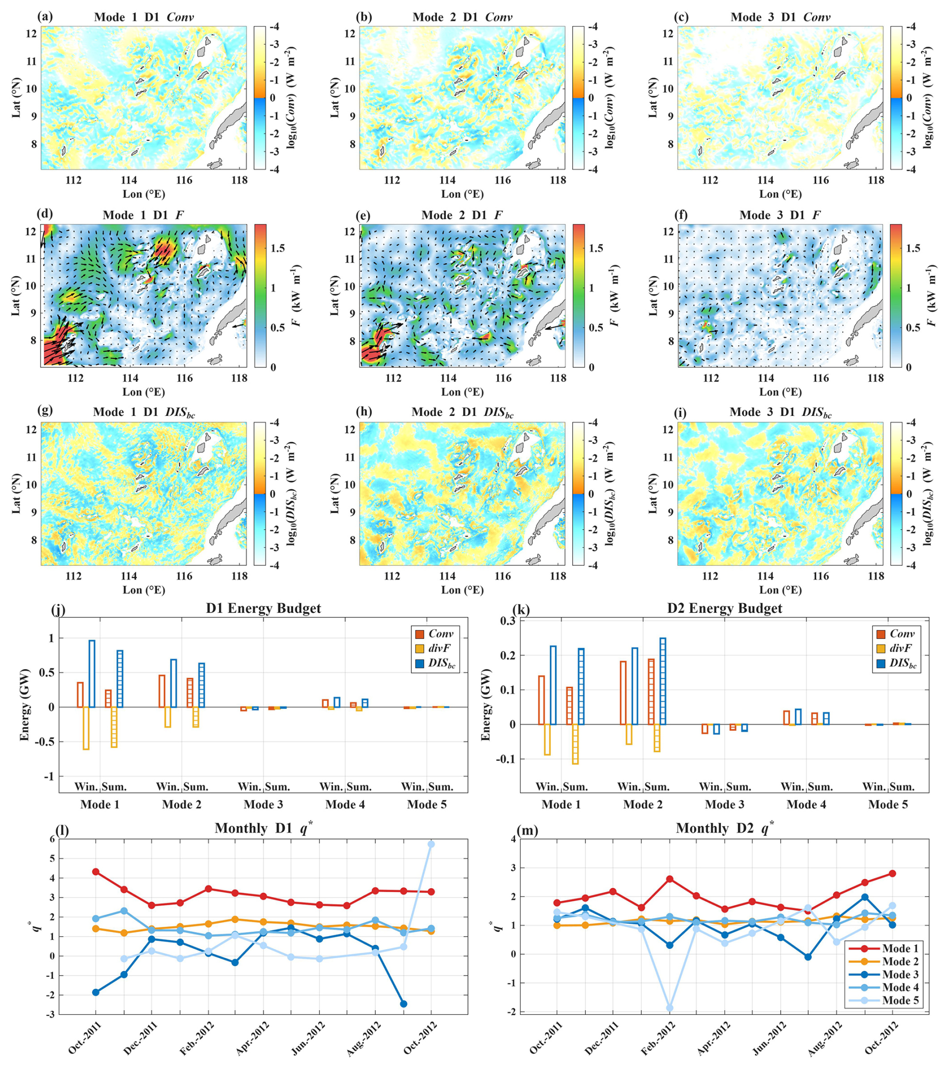
Figure 5 Same as Fig. 3, but for the Nansha Islands and (a–i) for diurnal internal tide.

In the Nansha Islands, all internal tidal energy budget terms decrease with increasing mode number, except for the mode-2 energy conversion (Fig. 5a–i). The mode-3 energy budget terms are generally less than one-third of those for modes 1–2. Two dominant incoming energy fluxes exist in the Nansha Islands, originating from the northeast and the southwest, respectively. With increasing mode number, the energy flux from the southwestern shelf slope of the SCS decays more rapidly than that from the northeastern source, suggesting that the reflection from the southwestern shelf slope of the SCS may furnish local dissipation in the Nansha Islands. Siyanbola et al. (2024) pointed out that in weak generation regions, intense local dissipation depends on sufficient convergence and slope reflection of far-field low-mode internal tidal beams. This is consistent with our results that the elevated mode-1 dissipation and q^* (>1) in the Nansha Islands are potentially dominated by the incoming mode-1 energy flux, particularly the reflection from the southwestern shelf slope of the SCS.

3.3 Parameterizations for the local dissipation ratio of internal tides

3.3.1 Parameterization constrained by physical factors

To develop parameterizations for q^* that are applicable to dynamically distinct regions, 3 key physical parameters are chosen based on the features of diurnal and semidiurnal tides in the LS and the Nansha Islands. The depth-averaged internal tidal shear (S²) within the bottommost 500 m represents the local internal wave intensity; the barotropic tidal kinetic energy (E_bt) quantifies the local tidal forcing strength; and the mode-1 internal tidal energy (E⁽¹⁾) is used to represent the potential for radiating low-mode energy to the far field. A dimensionless power-law function is fitted to the 429 d time series of q^* via multiple regression, with the specific formula expressed as

$$\begin{array}{}\text{(5)}& q_{\mathrm{para}}^{*}=q_{\mathrm{0}}{\left({\displaystyle \frac{S^{\mathrm{2}}}{S_{\mathrm{0}}^{\mathrm{2}}}}\right)}^{a_{\mathrm{1}}}{\left({\displaystyle \frac{E_{\mathrm{bt}}}{E_{\mathrm{bt}\mathrm{0}}}}\right)}^{a_{\mathrm{2}}}{\left({\displaystyle \frac{E^{\left(\mathrm{1}\right)}}{E_{\mathrm{0}}^{\left(\mathrm{1}\right)}}}\right)}^{a_{\mathrm{3}}}+q_{\mathrm{b}},\end{array}$$

where $S_{\mathrm{0}}^{\mathrm{2}}$, E_bt0 and $E_{\mathrm{0}}^{\left(\mathrm{1}\right)}$ are the time-mean reference values of each variable within each region; q₀ is the amplitude coefficient, q_b is a constant representing the background state; and a₁, a₂ and a₃ are the power-law exponents corresponding to the internal tidal shear, barotropic tidal kinetic energy, and mode-1 internal tidal energy, respectively.

Table 1 presents the fitted coefficients together with the coefficients of determination (R²) and root mean square error (RMSE) for this physical parameterization of q^* for diurnal and semidiurnal tides in both the LS and the Nansha Islands. R² and RMSE are indicators of the overall model performance rather than errors or uncertainties associated with individual coefficients. In the LS, R² for the diurnal and semidiurnal tides are both 0.35, with RMSE of 0.14 and 0.08, respectively. The fitted parameters characterize the dynamical process modulating q^* in the LS. For both diurnal and semidiurnal components, a₂ representing the sensitivity to barotropic tidal kinetic energy is positive (0.40 and 0.37, respectively), whereas a₃ representing the sensitivity to mode-1 internal tidal energy is negative (−0.31 and −0.40, respectively). Stronger local barotropic forcing therefore enhances internal tide generation and local dissipation, leading to a positive modulation of q^*. Conversely, when mode-1 internal tide energy accumulates substantially, the internal tide tends to propagate to the far field as coherent beams, thereby reducing q^* relatively. The background state constant q_b in the LS (0.05 and 0.15, respectively) is smaller than the amplitude coefficient q₀ (0.44 and 0.55, respectively). As shown in Fig. 6, the parameterization captures the mean state of q^* in the LS, although it exhibits some smoothing toward extreme values, manifesting as overestimation at low q^* and underestimation at high q^*.

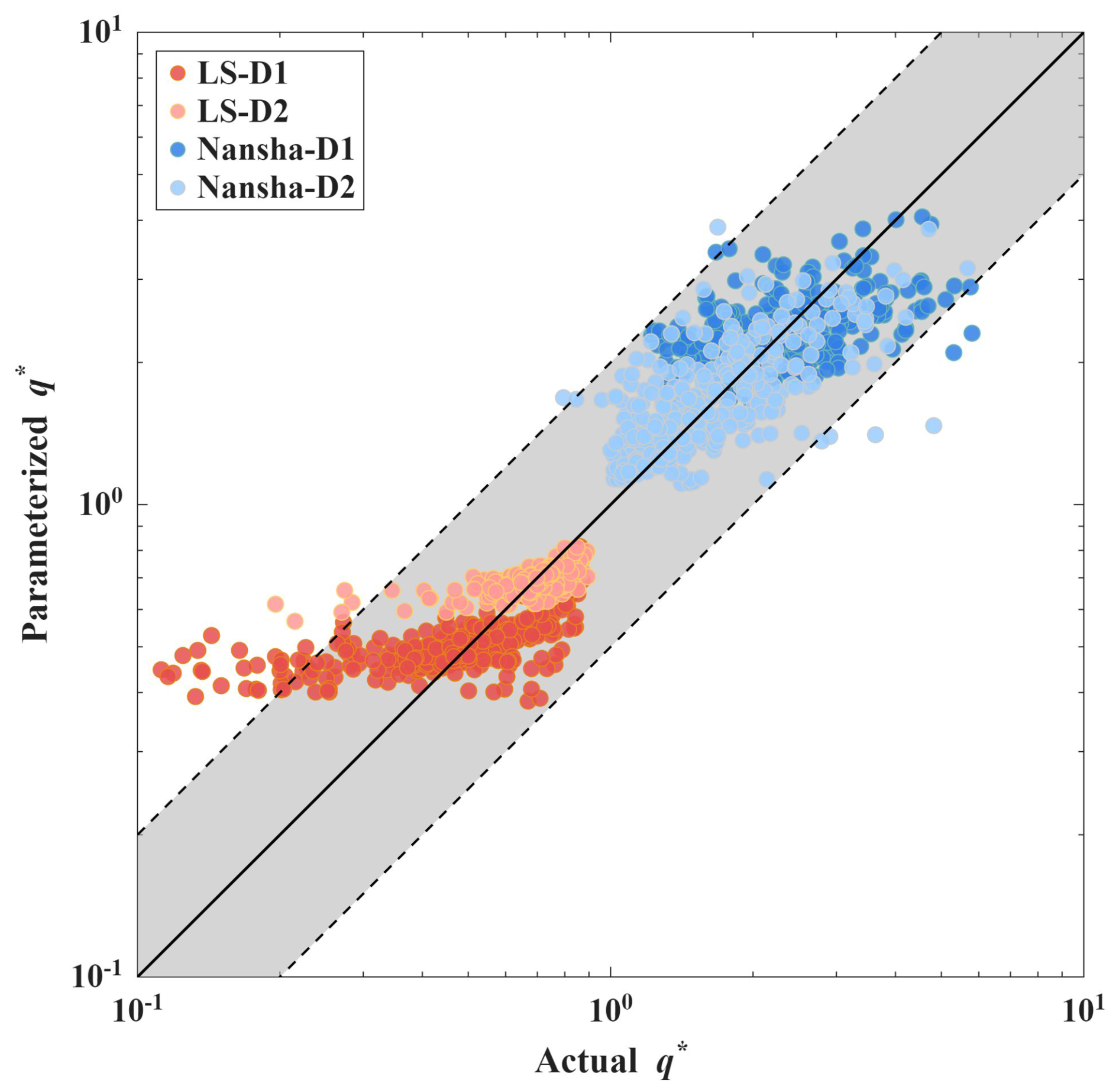
Figure 6 Scatter plot of parameterized q^* versus actual q^* for the LS and the Nansha Islands. The black line denotes the 1:1 reference line, and the two outer black dashed lines represent the 2:1 and 1:2 bounds.

Table 1 Fitted coefficients together with R² and RMSE of the physical parameterization for q^* in the LS and the Nansha Islands.

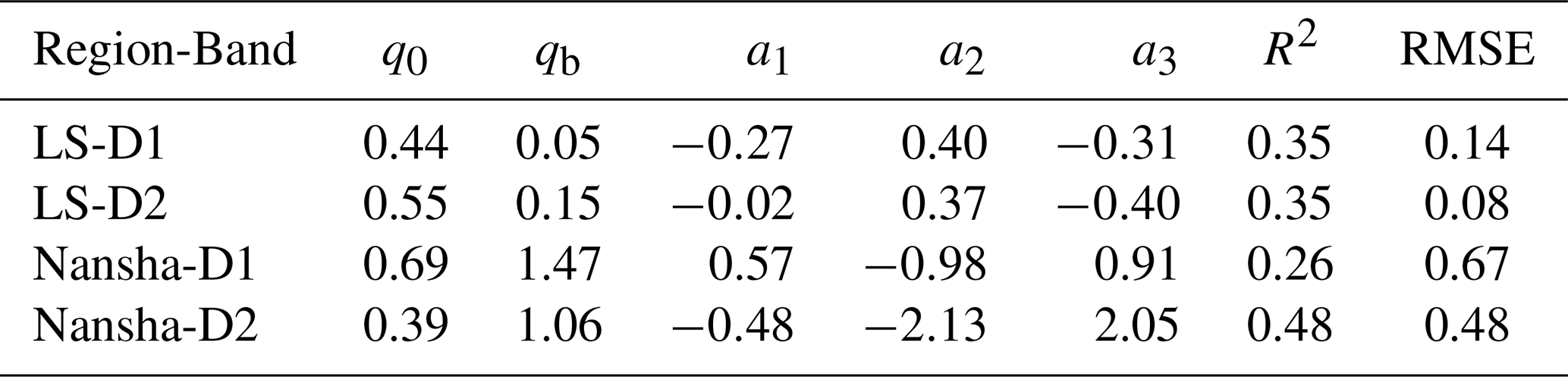
The parameterized q^* in the Nansha Islands reveals a dynamical process different from that of the LS. As shown in Table 1, the R² values for diurnal and semidiurnal tides are 0.26 and 0.48, respectively. For both diurnal and semidiurnal components, a₂ for barotropic tidal kinetic energy is negative (−0.98 and −2.13, respectively), whereas a₃ for mode-1 energy is positive (0.91 and 2.05, respectively). This indicates that when weakened local barotropic forcing reduces internal tide generation, q^* tends to increase, provided that the far-field low-mode energy remains elevated and drives intense local dissipation. a₁ for the internal tidal shear is negative for both diurnal and semidiurnal components in the LS (−0.27 and −0.02, respectively), whereas in the Nansha Islands it is positive for the diurnal component (0.57) and negative for the semidiurnal component (−0.48). The negative values do not indicate that enhanced internal tidal shear suppresses local dissipation; rather, the regionally averaged shear cannot capture local dissipation around the double ridges in the LS and the reefs in the Nansha Islands. In contrast to the LS, the background constants q_b for diurnal and semidiurnal tides in the Nansha Islands (1.47 and 1.06, respectively) substantially exceed the corresponding amplitude coefficients q₀ (0.69 and 0.39, respectively). This suggests that topographic scattering and reflection by the widespread seamounts and reefs, together with the incoming low-mode internal tidal energy, sustain q^* at a high level above 1.

3.3.2 Parameterization based on the XGBoost model

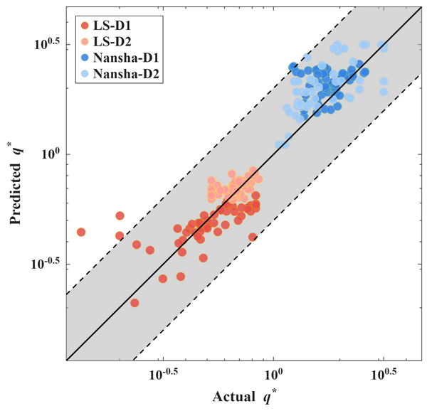
The XGBoost model achieves solid predictive performance on the combined testing set spanning both regions and tidal components, with an R² of 0.70 and an RMSE of 0.39 (Table 2). When predicting the semidiurnal component independently, the R² reaches 0.71. As shown in Fig. 7, the great overall performance of the model primarily stems from its ability to achieve clear macroscopic clustering across regions, separating the data into a low-q^* cluster for the LS and a high-q^* cluster for the Nansha Islands.

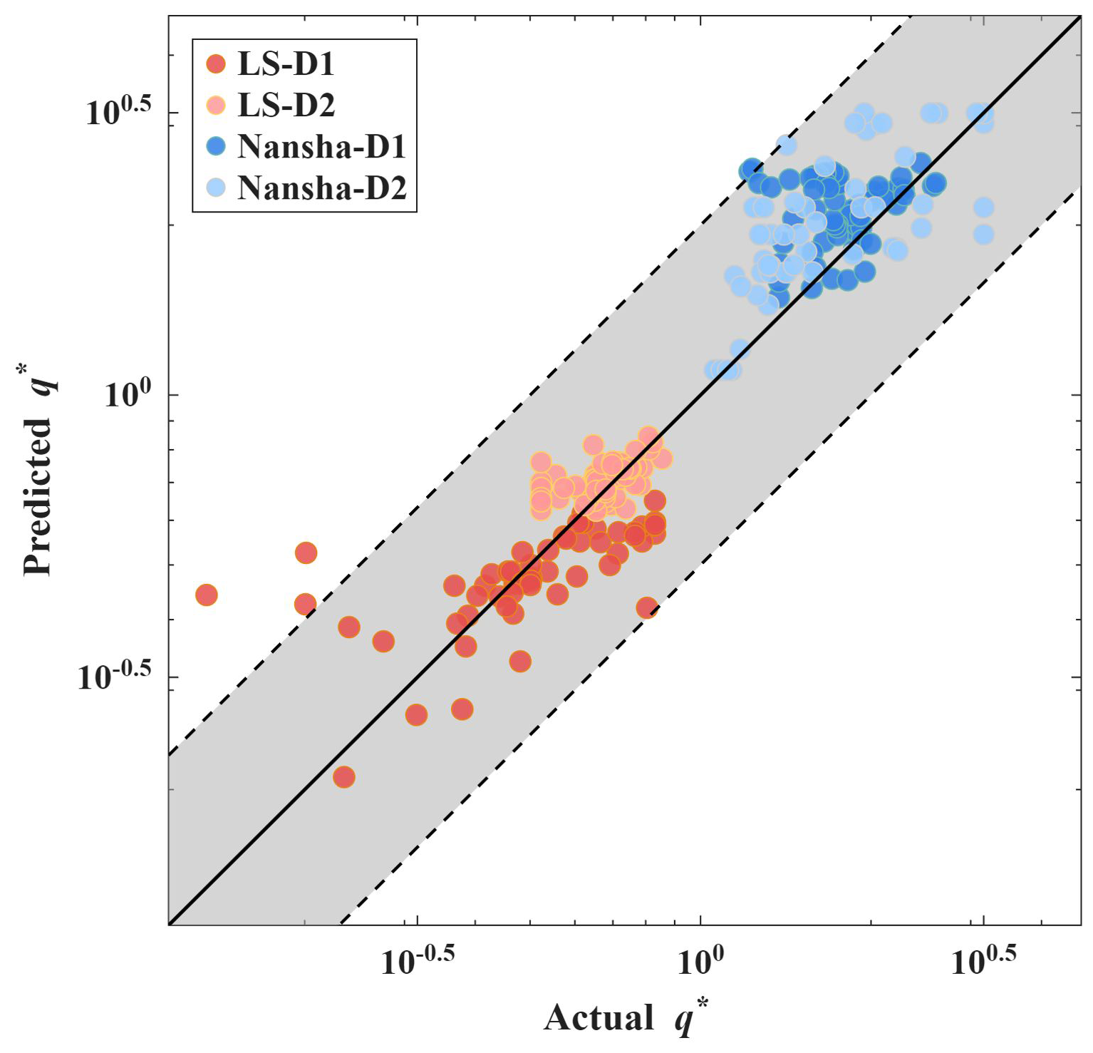
Figure 7 Scatter plot of the predicted q^* from the XGBoost model versus the actual q^* for the LS and the Nansha Islands. The black line represents the 1:1 reference line, and the two outer black dashed lines represent the 2:1 and 1:2 bounds.

Table 2 Performance of the XGBoost model on the testing set.

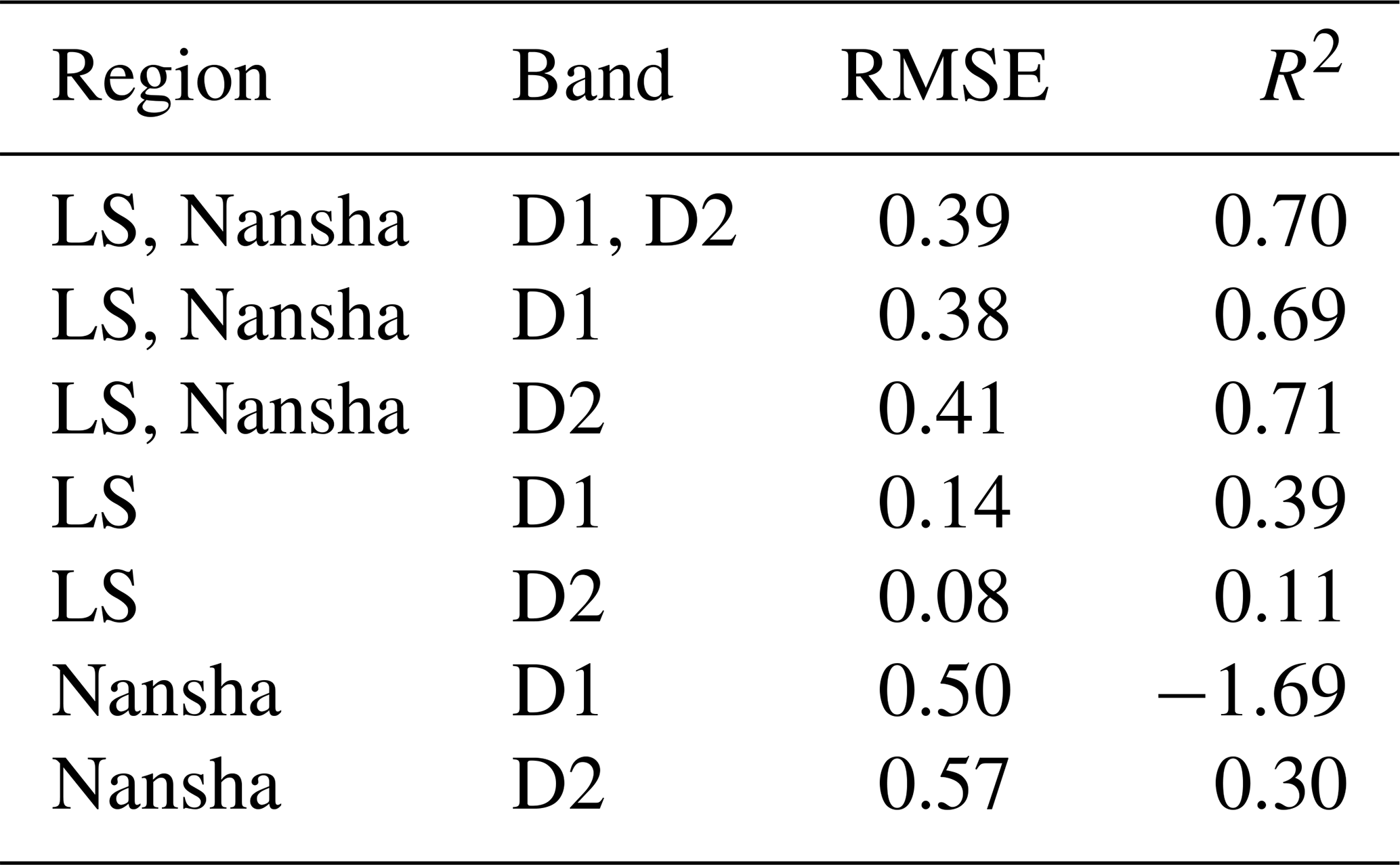
However, the predictive performance of the XGBoost model degrades markedly when predicting individual regions and tidal components separately. Table 2 shows that the R² values for diurnal and semidiurnal tides in the LS decrease to 0.39 and 0.11, respectively. The R² for the semidiurnal tide in the Nansha Islands is 0.30, and that for the diurnal tide is negative. As shown in Fig. 7, the model predictions for the LS are relatively concentrated and clustered along the 1:1 reference line, whereas those for the Nansha Islands exhibit greater dispersion. This degradation likely arises from the fact that extreme q^* values are highly sensitive to the topographic scattering of far-field low-mode internal tides and nonlinear wave-wave interactions.

As noted by Zhao et al. (2010), long-range internal tides form spatially complex interference patterns through superposition from multiple sources, with phase differences further modulated by mesoscale refraction. These far-field inputs and mesoscale processes are not captured by the local area-averaged input features employed here, which inevitably smooth out interference signals. Consequently, the XGBoost model broadly captures the phase of q^* variability over the spring-neap tidal cycles and predicts the temporal evolution of q^* well for the diurnal tide in the LS and the semidiurnal tide in the Nansha Islands (Fig. 8), although its predictions of q^* exhibit a degree of smoothing.

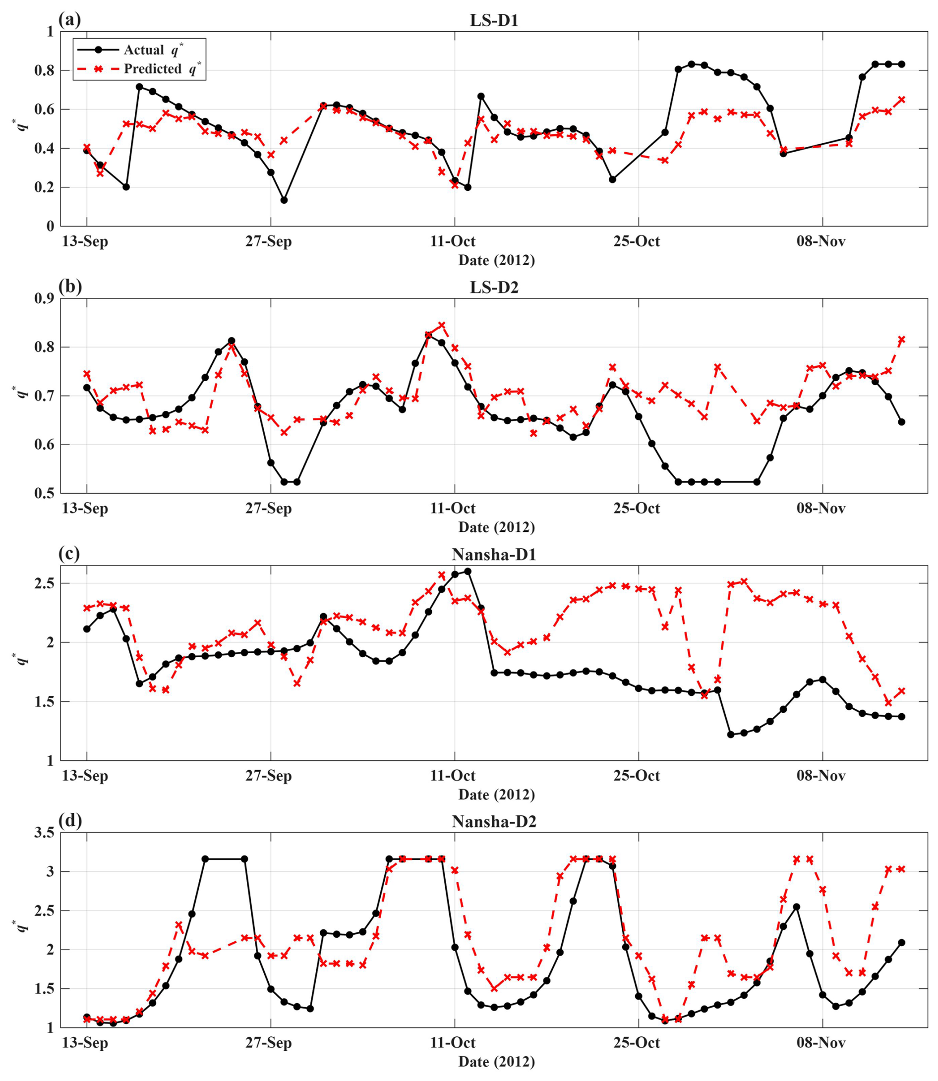
Figure 8 Time series of the predicted q^* from the XGBoost model and the actual q^* for the diurnal (D1) and semidiurnal (D2) tides in the LS and the Nansha Islands.

4 Summary

Based on the LLC4320 simulation, we reveal differences in the local internal tidal dissipation ratio (q^*) between the source region (represented by the LS) and the sink region (represented by the Nansha Islands). In the LS, the q^* value for the total internal tides ranges from 0.3 to 0.7, which is consistent with earlier results. The mode-1 energy flux radiates intensively out of the LS, resulting in mode-1 q^* values smaller than those of higher modes. This confirms that in generation regions of internal tides, much of the baroclinic energy propagates to the far field as low modes rather than dissipating locally. Conversely, in the Nansha Islands, q^* value for the total internal tides is generally larger than 1. In particular, the q^* values of the mode-1 diurnal and semidiurnal tides are consistently larger than those of higher modes. The reason for $q^{*}>\mathrm{1}$ is that the far-field internal tidal energy flux entering the Nansha Islands exceeds the locally generated one. Thus, the primary source for local dissipation is not the locally generated internal tide, but rather far-field internal tidal beams propagating from the LS.

The physical-based empirical formulation and the XGBoost model used to scale q^* in this study successfully capture the macroscopic clustering of the mean states of q^* in both the LS and the Nansha Islands. They also reproduce some of the periodic temporal variation of q^*, with an R² value reaching 0.70. Moreover, the physical parameterization results reveal regional differences in the dominant mechanisms modulating q^*. In the LS, while intense barotropic forcing generates energetic internal tides and enhances local dissipation, the substantial accumulation of mode-1 internal tidal energy favors the radiation of coherent beams into the far field, thereby reducing q^*. In the Nansha Islands, the negative power-law coefficient (a₂) for barotropic tidal kinetic energy, along with the positive coefficient (a₃) for mode-1 internal tidal energy, indicates that local dissipation is dominated by far-field energy input. Furthermore, the scattering and reflection of internal tides by the widespread seamounts and reefs play a dominant role in sustaining high q^* in the Nansha Islands. On the other hand, the XGBoost model yields a consistent periodic temporal change and accurately predicts the mean q^* value in both source and sink regions, despite some quantitative discrepancies. However, those far-field inputs and mesoscale processes are not captured by the local area-averaged input features, resulting in a degree of smoothing in the predicted q^*. This insight suggests that future parameterizations of q^* and internal tide mixing must move beyond the traditional framework that relies solely on local generation; instead, they should explicitly and thoughtfully incorporate the nonlocal processes, e.g., the far-field propagation of internal wave field experiencing interference and scattering.

The present study has several limitations. The horizontal grid spacing of LLC4320 is approximately 2 km in the study regions. At this resolution, the major topographic features and low-mode internal tides are explicitly resolved, whereas small-scale topographic features, the high-mode internal tides with short horizontal wavelengths, the internal wave breaking and the associated turbulence remain subgrid-scale processes and hence are not resolved. Therefore, internal tide generation driven by the unresolved roughness is absent from the simulation. Energy loss associated with unresolved scales may enter the model energy budget through parameterized viscosity and diffusivity and numerical damping, while bottom drag provides an additional explicit energy sink. In addition, because the present dissipation estimate (DIS_bc) is obtained as the residual of the simplified baroclinic energy budget equation, it may conflate dissipation associated with parameterized viscosity, diffusivity, and bottom drag; numerical mixing and damping. The archived model output does not permit an independent closure of the full energy budget, and these contributions cannot be quantified separately. Therefore, DIS_bc represents an inferred dissipation integrated over the study regions rather than diagnosed dissipation from the model at individual topographic features. Since DIS_bc appears in the numerator of q^*, its uncertainty propagates directly into the estimate of q^*. Crucially, the relative uncertainty of q^* is amplified where the area-integrated local conversion is weak. Such uncertainty is particularly pronounced over rough topography and for higher-mode internal tides (Vic et al., 2019). Future work with higher-resolution simulations and diagnostics of the individual dissipative terms is expected to separate and quantify these contributions.