LETKF-based Ocean Research Analysis version 2.0 for a quasi-global domain (LORA-QG): validation and intercomparison with eddy-permitting global ocean reanalysis datasets

We previously produced the local ensemble transform Kalman filter (LETKF)-based Ocean Research Analysis (LORA) version 1.0 datasets for the western North Pacific and Maritime Continent regions (LORA-WNP and LORA-MC, respectively) during the period from August 2015 to January 2024. However, these limited domains and periods constrain their applicability. Therefore, we developed a new eddy-permitting LETKF-based ocean data assimilation system and produced LORA version 2.0 for a quasi-global domain (LORA-QG) from June 2002, when the Advanced Microwave Scanning Radiometer (AMSR) series, a series of space-borne microwave imagers, began providing sea surface temperature observations and the Argo program substantially expanded in situ temperature and salinity measurements. We validated LORA-QG using observations from surface drifter buoys, tide gauges, and ocean climate stations, and compared the results with those of three eddy-permitting global ocean reanalysis datasets (GLORYS2V4, ORAS5, and C-GLORSv7). Although these observations are independent of LORA-QG, ORAS5, and C-GLORSv7, they are not entirely independent of GLORYS2V4. The validation results show that LORA-QG agrees well with the observations and has the second-highest accuracy among the four datasets in terms of overall root-mean-square deviations relative to the observations, thus achieving sufficient accuracy for geoscientific research and practical applications. LORA-QG provides features unavailable in conventional global reanalysis products, including ensemble-based uncertainty estimates and individual terms of the heat and salinity budget equations. These features make LORA-QG a valuable dataset for ensemble-based ocean forecasting and process-based studies. However, room for improvement remains, as LORA-QG exhibits significant warm biases in the tropics, particularly in the western tropical Pacific, and its sea surface salinity representation is likely limited due to relatively strong salinity nudging toward a climatological dataset in the mixed layer.

1 Introduction

Data assimilation produces accurate analysis datasets by combining numerical simulations and observations based on dynamical systems theory and statistical methods. Various research institutions and universities have developed ocean data assimilation systems and have produced analysis datasets useful for geoscience research and practical applications (e.g., Balmaseda et al., 2015; Martin et al., 2015). To the best of the authors' knowledge, eddy-resolving and eddy-permitting quasi-global and global reanalysis datasets that are currently distributed by actively maintained data services are summarized in Tables 1 and 2, respectively (as of August 2026). Nine eddy-resolving and eddy-permitting global and quasi-global datasets are available, and these adopt a variety of data assimilation methods, such as the three-dimensional variational method (3D-Var), optimal interpolation (OI), ensemble optimal interpolation (EnOI), and reduced-order Kalman filters.

Table 1 Overview of eddy-resolving quasi-global and global reanalysis datasets that are currently distributed by actively maintained data services (as of August 2026). The abbreviations are as follows: BRAN, Bluelink ReANalysis; GOFS3.1, Global Ocean Forecast System version 3.1; JCOPE-FGO, Japan Coastal Ocean Predictability Experiments-Forecasting Global Ocean; SODA, Simple Ocean Data Assimilation; CSIRO, Commonwealth Scientific and Industrial Research Organisation; JAMSTEC, Japan Agency for Marine-Earth Science and Technology; OFAM, Ocean Forecasting Australian Model; NEMO, Nucleus for European Modelling of the Ocean; HYCOM, Hybrid Coordinate Ocean Model; POM, Princeton Ocean Model; MOM5/1/SIS1, Modular Ocean Model; EnOI, ensemble optimal interpolation; SEEK, singular evolutive extended Kalman filter; 3D-Var, three-dimensional variational method; OI, Optimal interpolation; SST, sea surface temperature; and SSH, sea surface height. SEEK is a type of reduced-order Kalman filter.

¹ Oke et al. (2013), ² Madec and NEMO System Team (2024), ³ Metzger et al. (2014), ⁴ Mellor et al. (2002), ⁵ Griffies et al. (2015) and Winton et al. (2014),
⁶ Brasseur and Verron (2006) and Pham et al. (1998).

Table 2 Same as Table 1, but for eddy-permitting datasets, including LORA-QG (as of August 2026). The abbreviations are as follows: C-GLORSv7, CMCC Global Ocean Reanalysis System version 7; CMCC, Euro-Mediterranean Centre for Climate Change; LORA-QG, LETKF-based Ocean Research Analysis version 2.0 for a quasi-global domain; LETKF, local ensemble transform Kalman filter; ORAS5, Ocean ReAnalysis System 5; JAXA, Japan Aerospace Exploration Agency; ECMWF, European Centre for Medium-Range Weather Forecasts; sbPOM, Stony Brook Parallel Ocean Model; GFDL CM2.5, Geophysical Fluid Dynamics Laboratory Climate Model version 2.5; and SSS, sea surface salinity.

¹ Jordi and Wang (2012), ² Delworth et al. (2012), ³ Dee et al. (2011), ⁴ Hersbach et al. (2020), ⁵ Tsujino et al. (2018), ⁶ Hunt et al. (2007) and Miyoshi and Yamane (2007).

The ensemble Kalman filter (EnKF) has several advantages, including its flexibility in implementation with various numerical models, the ability to represent flow-dependent forecast error covariances, and the capability to conduct ensemble forecasts. The authors previously developed EnKF-based eddy-resolving ocean data assimilation systems (Fig. 1; Ohishi et al., 2022a, b, 2024a) and produced ensemble analysis datasets called the local-ensemble transform Kalman filter (LETKF)-based Ocean Research Analysis (LORA) version 1 for the western North Pacific and Maritime Continent regions (LORA-WNP and LORA-MC, respectively), covering August 2015–January 2024 (Ohishi et al., 2023, 2024b). Using the EnKF system, Ohishi et al. (2025) recently demonstrated that ensemble forecasts significantly outperform deterministic single-run forecasts for predicting the Kuroshio south of Japan. However, the ocean exhibits variability on interannual to decadal timescales, and the limited spatial and temporal coverage of LORA version 1 restricts its potential applications. Although Yin et al. (2011) developed an EnKF-based global ocean data assimilation system with 0.5° horizontal resolution that assimilates only in situ temperature and salinity profiles for the period 1979–2006, and more recently, Brassington et al. (2023) developed an eddy-resolving global EnKF system, these global ensemble analysis datasets are not publicly available (as of August 2026).

Figure 1 Domains of the local ensemble transform Kalman filter (LETKF)-based Ocean Research Analysis (LORA): the Maritime Continent (orange), western North Pacific (red), North Pacific (blue), and quasi-global (green) domains. Colors indicate topography derived from a 1 arcmin global relief model of Earth's surface (ETOPO1; Amante and Eakins, 2009).

The Advanced Microwave Scanning Radiometer for Earth Observing System (AMSR-E) aboard the Aqua satellite observed sea surface temperatures (SST) from June 2002 to October 2011 (Fig. 2a), and it provided near-global coverage within a day, except in regions affected by heavy rainfall, strong winds, or data gaps (Fig. 2b). Subsequently, AMSR2 aboard the Global Change Observation Mission–Water (GCOM-W) satellite has observed SST since July 2012, but there is a temporal gap between AMSR-E and AMSR2 (Fig. 2a). The WindSat polarimetric radiometer aboard the Coriolis satellite observed SST from August 2011 to October 2020 and partially bridged this gap, although its data coverage is more limited than that of AMSR-E and AMSR2 because of its narrower swath. Compared with microwave sensors, infrared sensors provide higher-spatial-resolution SST measurements but cannot observe SST under cloudy conditions, whereas microwave sensors can provide near-all-weather observations at the expense of coarser spatial resolution. Thus, these microwave SST observations have collectively enhanced global SST assimilation capabilities. Furthermore, since the 2000s, Argo profiling floats have dramatically enhanced in situ temperature and salinity observations in the global ocean.

Figure 2 (a) Timeline of microwave radiometer sensors: AMSR-E/Aqua (cyan), WindSat/Coriolis (green), AMSR2/GCOM-W (orange), and AMSR3/GOSAT-GW (gray). Daily composite SST from (b) AMSR-E, (c) WindSat, and (d) AMSR2 on 1 September 2011. (e)–(g) are the same as (b)–(d), respectively, but for 1 August 2012. The dotted lines in (a) indicate the dates of 1 September 2011 and 1 August 2012, corresponding to panels (b)–(d) and (e)–(g), respectively. The abbreviations are as follows: AMSR-E, Advanced Microwave Scanning Radiometer for Earth Observing System; GCOM-W, Global Change Observation Mission–Water; GOSAT-GW, Global Observing SATellite for Greenhouse gases and Water cycle; and SST, sea surface temperature.

Therefore, this study aims to develop an eddy-permitting EnKF-based ocean data assimilation system configured for a quasi-global domain (0–360° E, 70° S–70° N), to produce an analysis dataset from June 2002, and to evaluate its accuracy in comparison with existing eddy-permitting global reanalysis datasets. The resulting dataset is expected to provide a valuable resource for studies of ocean variability, mesoscale dynamics, and ocean predictability. Section 2 describes the experimental settings and validation methods, Sect. 3 presents the validation results, and Sect. 4 provides a summary and discussion.

2 Experimental settings and methods

2.1 EnKF-based quasi-global data assimilation system

This study extends the Stony Brook Parallel Ocean Model–local ensemble transform Kalman filter (sbPOM–LETKF) system previously configured for the western North Pacific and Maritime Continent regions (Ohishi et al., 2022a, b, 2024a) to a quasi-global domain. The model configuration and assimilation settings are summarized in Tables 3 and 4, respectively. To improve forecast accuracy and computational efficiency, several additional schemes and improvements were incorporated, as described below.

Table 3 Overview of the quasi-global ocean model configuration. The abbreviations are as follows: ETOPO1, a 1 arcmin global relief model of Earth's surface; WOA18, World Ocean Atlas 2018; SODA, Simple Ocean Data Assimilation; JRA55-do, Japanese 55-year atmospheric Reanalysis (JRA-55) based surface dataset for driving ocean-sea ice models; TE-Global, Today's Earth-Global; COARE, Coupled Ocean–Atmosphere Response Experiment.

¹ Amante and Eakins (2009), ² Locarnini et al. (2018) and Zweng et al. (2018), ³ Carton et al. (2018), ⁴ Ma et al. (2024), ⁵ Brodeau et al. (2017) and Edson et al. (2013), ⁶ Smagorinsky et al. (1965).

Table 4 Overview of the data assimilation configuration. The abbreviations are as follows: AMSR-E, Advanced Microwave Scanning Radiometer for Earth Observing System; GCOM-W, Global Change Observation Mission–Water; SMOS, Soil Moisture and Ocean Salinity; SMAP, Soil Moisture Active Passive; CMEMS, Copernicus Marine Service; GTSPP, Global Temperature and Salinity Profile Programme; AQC, Advanced automatic QC; RTPP, relaxation-to-prior perturbation; IAU, incremental analysis update; and AOEI, adaptive observation error inflation.

¹ https://gportal.jaxa.jp/gpr/?lang=en (last access: 10 September 2026), ² Shibata (2007), ³ https://www.esa.int/Applications/Observing_the_Earth/FutureEO/SMOS (last access: 10 September 2026), ⁴ Meissner et al. (2018), ⁵ https://doi.org/10.48670/moi-00146 (E.U. Copernicus Marine Service Information (CMEMS), 2026), ⁶ Sun et al. (2010), ⁷ https://pubargo.jamstec.go.jp/argo_product/catalog/aqc/catalog.html (last access: 10 September 2026), ⁸ Kotsuki et al. (2017) and Zhang et al. (2004), ⁹ Bloom et al. (1996), ¹⁰ Minamide and Zhang (2017).

2.1.1 Ocean model

We constructed a quasi-global ocean model covering 0–360° E and 70° S–70° N with horizontal resolution of 0.25° and 75 σ-layers using the Stony Brook Parallel Ocean Model (sbPOM; Jordi and Wang, 2012). The total grid size is $\mathrm{1442}\times \mathrm{562}\times \mathrm{75}$, which is approximately four and six times larger than those of the previous systems configured for the western North Pacific and Maritime Continent regions ($\mathrm{722}\times \mathrm{386}\times \mathrm{50}$ and $\mathrm{418}\times \mathrm{482}\times \mathrm{50}$, respectively). To improve forecast accuracy and computational efficiency, we substantially modified sbPOM. These modifications included modernizing legacy Fortran 77 code to Fortran 90 to improve code maintainability and readability, implementing Open Multi-Processing (OpenMP) parallelization and Parallel NetCDF input/output, and incorporating a scheme that subtracts and adds the horizontally averaged density before and after the pressure gradient calculation, respectively (Mellor et al., 1994).

The detailed model configuration is summarized in Table 3. We note that sea ice and tidal processes are not included in this model. To reduce pressure gradient errors (Mellor et al., 1994), a Gaussian filter with a 100 km e-folding scale is applied to the bottom topography. To prevent ensemble collapse (i.e., an excessive reduction of ensemble spread that can lead to filter divergence), the atmospheric and lateral boundary conditions, except for rainfall and river discharge, are perturbed (see Appendix 1 of Ohishi et al., 2023). The maximum ensemble size in this study is constrained by the maximum number of concurrent background jobs allowed per job submission on the Fugaku supercomputer at RIKEN and the Japan Aerospace Exploration Agency (JAXA) Supercomputer System Generation 3 (JSS3). We therefore set the ensemble size to 128, consistent with our previous regional systems (Ohishi et al., 2022a, b, 2023, 2024a, b). The ensemble simulation (i.e., spin-up) was conducted from an initial state of no motion for the period from January 1996 to May 2002, using the perturbed atmospheric and lateral boundary conditions and applying the full-depth temperature and salinity nudging with a 30 d timescale toward the monthly climatological dataset from the World Ocean Atlas 2018 (WOA18; Locarnini et al., 2018; Zweng et al., 2018).

2.1.2 Data assimilation

We used the LETKF (Hunt et al., 2007; Miyoshi and Yamane, 2007) to assimilate satellite SST, sea surface salinity (SSS), and sea surface height (SSH), as well as in situ temperature and salinity, at 1 d intervals. To improve computational efficiency, OpenMP parallelization was additionally implemented in the LETKF code, which has already been parallelized using MPI. The resulting system employs hybrid MPI/OpenMP parallelization.

The detailed assimilation configuration is summarized in Table 4. The mean dynamic ocean topography is estimated from the simulated SSH averaged over 1997–2001. Following Ohishi et al. (2022a, b), we adopt a combination of the incremental analysis update (IAU; Bloom et al., 1996), relaxation-to-prior perturbation (RTPP; Kotsuki et al., 2017; Zhang et al., 2004), and adaptive observation error inflation (AOEI; Minamide and Zhang, 2017) to improve dynamical balance and analysis accuracy. In RTPP, forecast ensemble perturbations are relaxed toward analysis ensemble perturbations with a relaxation coefficient of 0.9. Following Miyazawa et al. (2012) and Penny et al. (2013), covariance localization is applied in observation space using a Gaussian function with horizontal and vertical localization scales of 300 km and 100 m (corresponding to cutoff scales of 1100 km and 370 m, respectively).

Using the Fugaku and JSS3 supercomputers, which consist of the Fujitsu PRIMEHPC FX1000, we have integrated the system since 1 June 2002, when AMSR-E/Aqua started SST observations. To suppress SSS drift, we applied salinity nudging toward the WOA18 monthly climatology with a 30 d timescale in the mixed layer, whereas no nudging was applied to temperature. When 512 nodes (24 576 CPUs) are used with hybrid Message Passing Interface (MPI)/OpenMP parallelization, one assimilation cycle requires approximately 20–30 min. We output the daily mean three-dimensional (3D) ensemble mean and spread, as well as the daily mean two-dimensional (2D) fields of all ensemble members at the sea surface. The data volume of the 3D ensemble mean and spread is approximately 100 GB per month, when individual terms of the temperature and salinity budget equations are saved in addition to the basic variables (e.g., temperature, salinity, and SSH). The data volume of the 2D surface fields for all ensemble members is approximately 30 GB per month, when only the basic variables are saved. The resulting analysis dataset is referred to as the LETKF-based Ocean Research Analysis version 2.0 for a quasi-global domain (LORA-QG).

2.2 Validation

Since data assimilation may degrade analysis accuracy substantially through the accumulation of negative effects from initial shocks, especially with frequent assimilation (Ohishi et al., 2022b), we first evaluate the annual climatological temperature and salinity fields and their analysis biases relative to the observational climatological dataset, the World Ocean Atlas 2018 (WOA18; Locarnini et al., 2018; Zweng et al., 2018) (see Sect. 3.1). We further validate LORA-QG by comparing analysis biases and root-mean-square deviations (RMSDs) relative to observations listed in Table 5 with those from three eddy-permitting global ocean reanalysis datasets that have similar resolution, domain, and output intervals (Table 2), with the exception of Simple Ocean Data Assimilation version 3 (SODA3; Carton et al., 2018): CMCC Global Ocean Reanalysis System version 7 (C-GLORSv7; Storto et al., 2016), GLORYS2V4 (Lellouche et al., 2013), and Ocean ReAnalysis System 5 (ORAS5; Zuo et al., 2019) (see Sects. 3.2–3.4). All of the observations are independent of LORA-QG, C-GLORSv7, and ORAS5. However, SST from the drifter buoys and temperature and salinity from the Ocean Climate Stations are not independent of GLORYS2V4 (Table 5). When quality-control flags are available, observations flagged as bad quality are excluded from the validation. All validations are performed in observation space using daily-averaged ensemble-mean fields from LORA-QG and daily-mean fields from C-GLORSv7, GLORYS2V4, and ORAS5 reanalysis datasets. The validation period covers January 2003–December 2023.

Table 5 Observations used for validation. The abbreviations are as follows: NOAA, National Oceanic and Atmospheric Administration; UHSLC, University of Hawaii Sea Level Center; KEO, Kuroshio Extension Observatory; PMEL, Pacific Marine Environmental Laboratory.

¹ https://www.aoml.noaa.gov/global-drifter-program/ (last access: 10 September 2026; ² https://uhslc.soest.hawaii.edu/ (last access: 10 September 2026); ³ https://www.pmel.noaa.gov/ocs/ (last access: 10 September 2026).

To clarify the differences relative to LORA-QG, we also calculate the absolute bias differences and RMSD ratios defined as $\left|{\text{bias}}_{\text{anal}}\right|-\left|{\text{bias}}_{\text{LORA-QG}}\right|$ and $\mathrm{100}\times ({\text{RMSD}}_{\text{anal}}-{\text{RMSD}}_{\text{LORA-QG}})/{\text{RMSD}}_{\text{LORA-QG}}$, respectively. Here, $|\cdot |$ denotes the absolute value, the subscript anal represents the GLORYS2V4, ORAS5, and C-GLORSv7 datasets, and the subscript LORA-QG represents the LORA-QG dataset. Statistically significant differences in the absolute analysis biases and RMSDs relative to LORA-QG are identified at a 99 % confidence level, using a bootstrap method with 1000 resampling iterations applied to the monthly absolute bias and RMSD differences.

Figure 3 Annual SST climatology from (a) WOA18 (colors and contours), (b) LORA-QG, (c) GLORYS2V4, (d) ORAS5, and (e) C-GLORSv7 (contours) for the period 2003–2023. In (b)–(e), the colors indicate analysis biases relative to WOA18. Thin and thick contour intervals are 2 and 10 °C, respectively. The abbreviations are as follows: SST, sea surface temperature; WOA18, World Ocean Atlas 2018; LORA-QG, LETKF-based Ocean Research Analysis version 2.0 for a quasi-global domain; LETKF, local ensemble transform Kalman filter; ORAS5, Ocean ReAnalysis System 5; C-GLORSv7, CMCC Global Ocean Reanalysis System version 7; and CMCC, Euro-Mediterranean Centre for Climate Change.

Figure 4 Same as Fig. 3, but for meridional sections of annual temperature climatology averaged over the global ocean, excluding 0–60° E to avoid the influence of high-salinity water in the Mediterranean Sea on the zonal mean.

3 Results

3.1 Annual temperature and salinity climatology validation using WOA18

As described in Sect. 2.2, data assimilation may substantially degrade analysis accuracy through the accumulation of initial shocks; therefore, we first examine the annual climatological temperature and salinity fields at the sea surface (Figs. 3 and 5) and their globally averaged meridional sections (Figs. 4 and 6), excluding 0–60° E, where the regionally confined high-salinity waters in the Mediterranean Sea strongly affect the zonal mean. The annual SST climatological fields of all four analysis products are generally consistent with WOA18 (contours in Fig. 3), although warm SST biases are distributed over wide areas (colors in Fig. 3). The temperature meridional sections indicate that these warm biases are mostly confined to the near-surface layer (Fig. 4). LORA-QG exhibits warm and cool biases in the bottom layer and at depths of 100–2000 m between 60 and 70° S, respectively (Fig. 4b), whereas the other datasets show the opposite patterns (Fig. 4c–e).

Figure 5 Same as Fig. 3, but for annual sea surface salinity (SSS) climatology for the period 2003–2023. Thin and thick contour intervals are 0.5 and 2, respectively.

Figure 6 Same as Fig. 4, but for meridional sections of annual salinity climatology. Thin and thick contour intervals are 0.5 and 2, respectively.

The annual SSS climatological fields of all four products are also generally consistent with WOA18 (contours in Fig. 5), but SSS biases in LORA-QG are generally smaller than those in the other three datasets (colors in Fig. 5), likely reflecting the relatively strong salinity nudging applied in the mixed layer (Sect. 2.1.2). The salinity meridional section shows that low- and high-salinity biases are distributed at depths of 1000–3500 m and 3500–5000 m, respectively, only in LORA-QG (Fig. 6). These temperature and salinity biases in the ocean interior are likely associated with the limited availability of observations, data assimilation schemes, and model-related factors, including the vertical localization in LETKF, the specification of lateral boundary conditions from SODA3, limitations in representing high-latitude processes such as Antarctic Bottom Water formation, and differences in vertical mixing schemes: the Nakanishi and Niino (2009) level 2.5 scheme used in LORA-QG and the turbulence kinetic energy (TKE)-based level 1.5 closure scheme used in the other datasets. However, a more detailed investigation is beyond the scope of this study. Therefore, all four datasets reproduce the annual temperature and salinity climatological fields reasonably well overall.

3.2 Surface horizontal currents and SST validation using surface drifter buoys

To validate surface horizontal currents and SST, we calculated temporally averaged analysis RMSDs and biases relative to the independent surface drifter buoys in 5° longitude × 5° latitude bins for the quasi-global domain (0–360° E, 70° S–70° N) (panels a–d of Figs. 7–10), as well as corresponding RMSD ratios and absolute bias differences (panels f–h of Figs. 7–10), spatially averaged monthly analysis RMSDs (Fig. 11), and spatiotemporally averaged analysis RMSDs (shown at the bottom of Figs. 7a–d and 9a–d). For all four analysis datasets, large RMSDs in surface zonal velocity are found in dynamically active regions, such as the western boundary currents, Antarctic Circumpolar Current (ACC), and tropical instability waves (Fig. 7a–d). As shown at the bottom of Fig. 7a–d, the spatiotemporally averaged RMSD of LORA-QG is 0.172 m s⁻¹, which is significantly larger than that of GLORYS2V4 (0.154 m s⁻¹) and significantly smaller than those of ORAS5 and C-GLORSv7 (0.197 and 0.192 m s⁻¹, respectively). These results are supported by the RMSD ratio maps, which show that GLORYS2V4 generally outperforms LORA-QG in most regions, whereas the opposite is true for ORAS5 and C-GLORSv7.

Figure 7 Temporally averaged analysis root-mean-square deviations (RMSDs) of (a) LORA-QG, (b) GLORYS2V4, (c) ORAS5, and (d) C-GLORSv7 relative to surface zonal velocities from drifter buoys in 5° longitude × 5° latitude bins for the quasi-global domain (0–360° E, 70° S–70° N). (e) Same as (a), but for the analysis ensemble spread. (f–h) Same as (b)–(d), but for the RMSD ratios defined in Sect. 2.2. In (a)–(h), bins with an observation availability of less than 1 per month are shown in white. In (a)–(d), spatiotemporally averaged RMSDs are shown at the bottom, and the bold italic font indicates statistically significant differences from LORA-QG at a 99 % confidence level. In (e), the color scale is the same as that in (a) for direct comparison. In (f)–(h), red and blue colors denote that LORA-QG reproduces the drifter buoy observations better and worse than the other datasets, respectively; dot marks indicate statistically significant differences from LORA-QG at the 99 % confidence level.

Figure 8 (a–d) Same as Fig. 7a–d, but for temporally averaged analysis biases. (e) The observation availability of the surface drifter buoys. (f–h) Same as Fig. 7f–h, but for the absolute bias differences relative to LORA-QG. In (f)–(h), red and blue colors denote that the absolute biases in LORA-QG are smaller and larger than those of the other datasets, respectively; dot marks indicate statistically significant differences in the absolute biases at the 99 % confidence level.

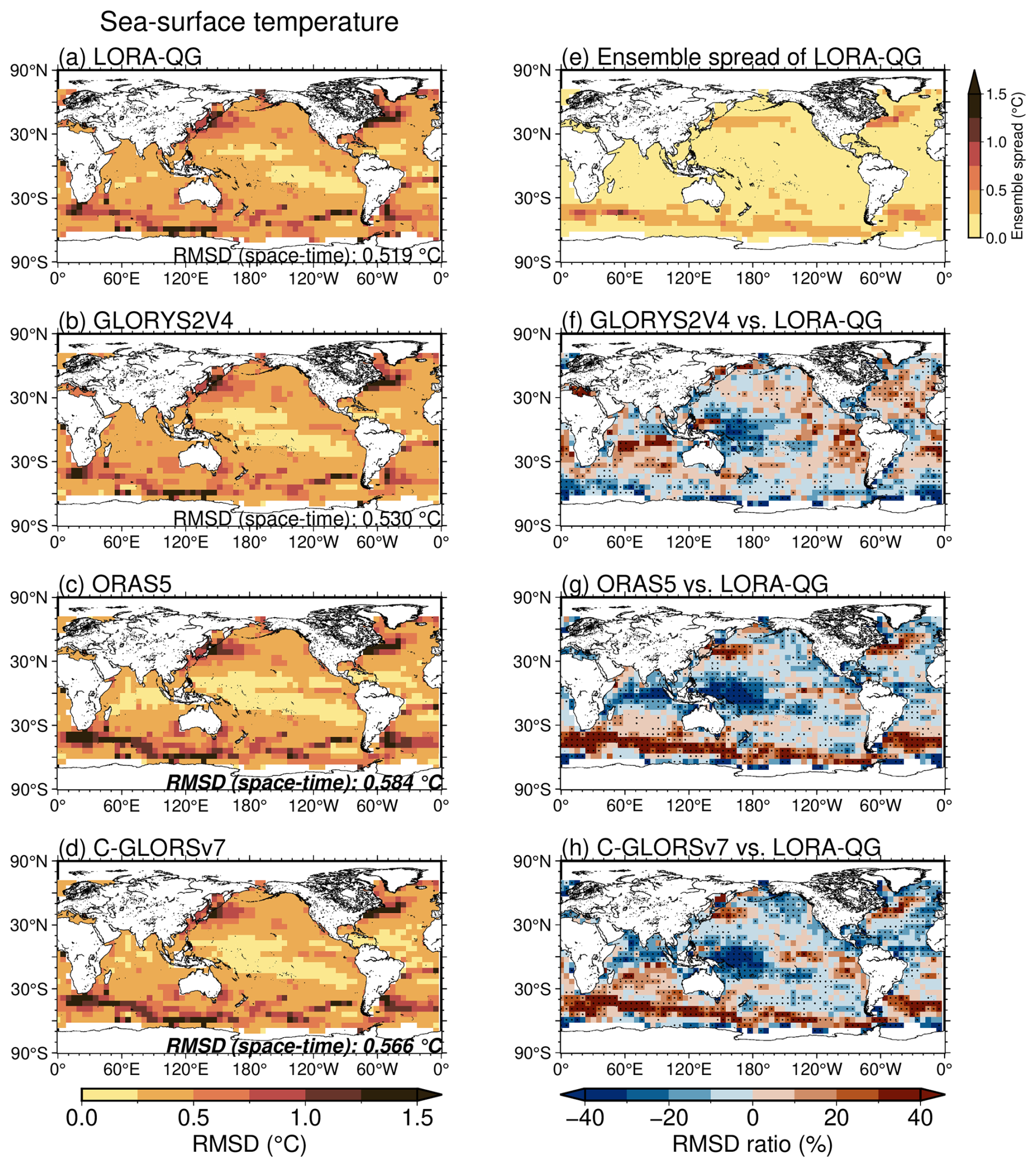
Figure 9 Same as Fig. 7, but for SST.

Figure 10 Same as Fig. 8, but for SST.

Figure 11 Spatially averaged monthly analysis RMSDs of LORA-QG (black), GLORYS2V4 (cyan), ORAS5 (orange), and C-GLORSv7 (green) relative to surface (a) zonal velocity, (b) meridional velocity, and (c) SST from the drifter buoys. In (a)–(c), the black dashed line indicates the corresponding spatially averaged monthly analysis ensemble spread of LORA-QG. (d) Total numbers of surface zonal velocity (black), meridional velocity (cyan), and SST (orange) observations from the drifter buoys.

GLORYS2V4, ORAS5, and C-GLORSv7 exhibit substantial biases that tend to weaken the large-scale general circulation, with positive and negative biases weakening the westward and eastward currents in subtropical and mid-latitude regions, respectively (Fig. 8b–d), whereas LORA-QG does not show such systematic bias patterns (Fig. 8a). Compared with LORA-QG, the absolute biases in GLORYS2V4 are significantly larger in the Southern Ocean and western tropical Pacific, and those in ORAS5 and C-GLORSv7 are significantly larger in most regions. In the eastern tropical Pacific and tropical Atlantic, the absolute biases in LORA-QG are significantly larger than those of the other three datasets.

The validation results for the surface meridional velocity are qualitatively similar to those for the surface zonal velocity (figures not shown). The spatiotemporally averaged RMSD of LORA-QG is 0.160 m s⁻¹, which is significantly larger than that of GLORYS2V4 (0.144 m s⁻¹) and significantly smaller than those of ORAS5 and C-GLORSv7 (0.182 and 0.180 m s⁻¹, respectively). These results indicate that the accuracy of the surface horizontal currents generally ranks in the order of GLORYS2V4 > LORA-QG > C-GLORSv7 > ORAS5.

Large SST RMSDs are distributed around frontal regions such as the western boundary currents and ACC for all analysis products (Fig. 9a–d). The spatiotemporally averaged RMSD of LORA-QG is 0.519 °C, which is smaller than that of GLORYS2V4 (0.530 °C), although the difference is not statistically significant, whereas it is significantly smaller than those of ORAS5 and C-GLORSv7 (0.584 and 0.566 °C, respectively) (bottom of Fig. 9a–d). The RMSDs of LORA-QG are significantly larger than those of the other three datasets in the tropics, especially in the western tropical Pacific (Fig. 9f–h), while they are significantly smaller than those of ORAS5 and C-GLORSv7 around the western boundary currents and ACC (Fig. 9g and h). No pronounced large-scale structures are evident in the RMSD differences between LORA-QG and GLORYS2V4 (Fig. 9f), consistent with the lack of statistical significance in their spatiotemporally averaged differences. Flow-dependent forecast error covariance in LORA-QG and GLORYS2V4 might capture the mesoscale variations better and result in the smaller RMSDs around the western boundary currents and ACC compared with the static error covariance in ORAS5 and C-GLORSv7.

LORA-QG exhibits significant warm SST biases primarily in the tropics, especially in the western tropical Pacific (Fig. 10a and f–h), which contribute substantially to its large RMSDs (Fig. 9a). GLORYS2V4 and ORAS5 show widespread cool SST biases across the global ocean, with the biases being particularly pronounced in ORAS5. The bias differences of LORA-QG with GLORYS2V4 and ORAS5 may reflect differences in both the ocean model and assimilation configurations (Table 2), such as vertical mixing parameterizations and data assimilation schemes. In particular, the warm biases of LORA-QG may be related to limitations in microwave SST observations. Microwave SST retrievals are generally considered to represent the subskin temperature and can differ from the skin temperature observed by infrared sensors. In addition, microwave SST retrievals are affected by precipitation and can introduce systematic errors under heavy rainfall conditions. The spatial distribution of the warm biases in LORA-QG is broadly consistent with that of the rainfall climatology (cf. https://gpm.nasa.gov/data/imerg/precipitation-climatology, last access: 10 September 2026), suggesting that precipitation-related retrieval errors may contribute to the warm biases. In contrast, the other three datasets assimilate optimally interpolated SST products that combine infrared and microwave satellite observations, which may help mitigate such precipitation-related errors.

The time series of the globally averaged RMSDs indicate that the RMSD of the surface horizontal currents is the smallest for GLORYS2V4, followed by LORA-QG, and then C-GLORSv7 and ORAS5 over the entire analysis period (Fig. 11a and b). During the first half of the analysis period (2005–2011), the SST RMSD is the smallest for GLORYS2V4, followed by LORA-QG, C-GLORSv7, and ORAS5. In 2011–2012, when SST assimilation in LORA-QG is limited to WindSat (Fig. 2), the RMSD of LORA-QG increases; however, during the latter half of the analysis period (2015–2020), it becomes the smallest, likely reflecting the assimilation of the two microwave satellite SST data (WindSat and AMSR2). Thus, the SST RMSDs are the smallest for GLORYS2V4 during 2005–2011 and for LORA-QG during 2015–2020, which is consistent with the absence of statistically significant differences between them.

For LORA-QG, both the spatially and temporally averaged ensemble spreads of surface horizontal currents and SST (Figs. 7e, 9e, and 11a–c) are substantially smaller than the corresponding RMSDs over the entire analysis period and domain (Figs. 7a, 9a, and 11a–c), even when accounting for observation errors in the drifter buoy data. This indicates that the ensemble spread is underestimated. Consequently, although the EnKF system in this study introduces perturbations in the atmosphere and lateral boundary conditions and maintains ensemble spread using RTPP, additional inflation is required to further increase the ensemble spread.

Since the drifter buoy observations themselves may also influence the validation results, we examined their spatial and temporal distributions (Figs. 8e, 10e, and 11d). Although the number of drifter buoy observations varies across time and space and may be limited in the tropics and Southern Ocean, as well as during the periods 2003–2005, 2012–2014, and 2022–2023, there are almost no bins with an observation availability smaller than 1 per month over the quasi-global analysis domain. Therefore, sampling effects associated with the drifter buoy distribution are unlikely to substantially affect the overall validation results.

3.3 Sea level validation using tide gauge stations

We calculated temporally averaged RMSDs of the four analysis datasets relative to sea level anomalies from the independent tide gauge stations (Fig. 12a–d), as well as the corresponding RMSD ratios (Fig. 12f–h), station- and temporally averaged RMSDs (shown at the bottom of Fig. 12a–d), and the temporally averaged ensemble spread of LORA-QG (Fig. 12e). Here, at each station, the analysis SSH is defined as the model grid value closest to the station within a 100 km radius, and the reference level is set to 0 m for all observation and analysis datasets by subtracting each own temporal SSH average over the period when all observation and analysis datasets exist.

Figure 12 Same as Fig. 7, but for sea level anomalies from the tide gauge stations. In (a)–(d), station- and temporally averaged RMSDs are shown at the bottom. In (a), green, yellow, and cyan circles indicate the Tauranga, Kukup, and Booby Island stations, respectively, which are used to illustrate the time series of sea level anomalies in Fig. 13. In (f)–(h), circle marks indicate statistically significant differences from LORA-QG at the 99 % confidence level, whereas cross marks denote statistically no significant differences.

The RMSDs of LORA-QG, GLORYS2V4, and ORAS5 tend to be smaller in the tropics than in mid- to high-latitude regions (Fig. 12a–c). The RMSDs of C-GLORSv7 are substantially larger than those of the other three datasets at almost all stations (Fig. 12d), and this issue is discussed further below. The station- and temporally averaged RMSD of LORA-QG is 0.0888 m, which is significantly larger than those of GLORYS2V4 and ORAS5 (0.0748 and 0.0803 m, respectively) but significantly smaller than that of C-GLORSv7 (0.2227 m). These results are supported by the RMSD ratio maps (Fig. 12f–h). At most stations, the RMSDs of LORA-QG are significantly larger than those of GLORYS2V4 and ORAS5 (Fig. 12f and g), whereas they are significantly smaller than those of C-GLORSv7 (Fig. 12h).

Figure 13 shows the time series of the sea level anomalies from the tide gauge observations and analysis datasets at the Tauranga station (green circle in Fig. 12a), where the RMSD of LORA-QG is closest to its station- and temporally averaged RMSD, and at the Kukup and Booby Island stations (yellow and cyan circles in Fig. 12a, respectively), which have the smallest and largest RMSD ratios. For all three stations, a substantial decreasing trend in sea level is found in C-GLORSv7, resulting in significantly large RMSDs (green lines in Fig. 13). This issue is likely related to a global freshwater budget imbalance due to the lack of an explicit constraint on the total ocean volume (personal communication with A. Cipollone). Small inconsistencies in surface freshwater fluxes and other boundary forcings may accumulate over time, leading to a spurious drift in the global mean SSH. In contrast, such a drift is not evident in LORA-QG, likely because the assimilated SSH data consist of a combination of the simulated SSH climatology and satellite-derived SSH anomalies, and because the analysis increments are applied only to temperature, salinity, and horizontal velocities through the IAU.

Figure 13 Sea level anomalies of tide gauge observations (black), LORA-QG (blue), GLORYS2V4 (cyan), ORAS5 (orange), and C-GLORSv7 (green) at (a) the Tauranga station, where the RMSD of LORA-QG is closest to its station- and temporally averaged RMSD (green circle in Fig. 12a), and at the (b) Kukup and (c) Booby Island stations, which have the smallest and largest RMSD ratios (yellow and cyan circles in Fig. 12a, respectively).

At the Tauranga station, the other three analysis datasets reasonably reproduce the tide gauge observations (Fig. 13a). At the Kukup station, LORA-QG reproduces the observations more closely than GLORYS2V4 and ORAS5, as the amplitudes of the latter two datasets are larger than those of the observations (Fig. 13b). At the Booby Island station, the results are opposite to those at the Kukup station (Fig. 13c). For these two stations, the Indonesian Throughflow and seasonal winds may play important roles in controlling sea level variability. A more detailed investigation of these processes is beyond the scope of this study and is left for future work.

3.4 Ocean interior validation using ocean climate stations

Based on daily-mean observations of ocean interior temperature, salinity, zonal velocity, and meridional velocity observed from the independent KEO and Papa buoys (Fig. 14a), we calculated temporally averaged analysis RMSDs and biases (panels a and b of Figs. 15–18, respectively), temporally and depth-averaged analysis RMSDs (triangles at the bottom of panel a in Figs. 15–18), and the corresponding RMSD ratios and absolute bias differences (panels c and d of Figs. 15–18). The observations at the KEO buoy are available from 16 June 2004 for temperature and salinity and from 30 May 2005 for horizontal velocity, and those at the Papa buoy are available from 8 June 2007 for temperature, salinity, and velocity. Data points with less than 20 % availability are excluded (Fig. 14b–i).

Figure 14 (a) Positions of the Kuroshio Extension Observatory (KEO; orange) and Papa (cyan) buoys. Observation availability for (b) temperature, (c) salinity, (d) zonal velocity, and (e) meridional velocity at the KEO buoy. (f–i) Same as (b)–(e), but for the Papa buoy. In (b)–(i), the dotted lines indicate the 20 % threshold.

Figure 15 Temporally averaged analysis (a) RMSDs and (b) biases of LORA-QG (black), GLORYS2V4 (cyan), ORAS5 (orange), and C-GLORSv7 (green) relative to temperature observations at the KEO buoy. (c) RMSD ratios and (d) absolute bias differences of GLORYS2V4 (cyan), ORAS5 (orange), and C-GLORSv7 (green). In (a), the dashed black line indicates the temporally averaged analysis ensemble spread, and triangles at the bottom denote the temporally and depth-averaged analysis RMSDs. Open triangles in (a) and open circles in (c) and (d) indicate statistically significant differences from LORA-QG at the 99 % confidence level. In (c) and (d), positive and negative values indicate that LORA-QG reproduces the KEO buoy observations better and worse than the other reanalysis datasets, respectively.

Figure 16 Same as Fig. 15, but for salinity at the KEO buoy.

Figure 17 Same as Fig. 15, but for temperature at the Papa buoy. The ranges of the horizontal and vertical axes differ from those in Fig. 15.

Figure 18 Same as Fig. 15, but for salinity at the Papa buoy. The ranges of the horizontal and vertical axes differ from those in Fig. 16.

3.4.1 KEO buoy

Throughout the observed depth range at the KEO buoy, the temperature analysis RMSDs of LORA-QG are significantly larger than those of GLORYS2V4 (Fig. 15a and c). They are significantly smaller than those of C-GLORSv7 only in the upper 0–100 m, but are nearly identical at depths below 100 m. Compared with ORAS5, the RMSDs of LORA-QG are significantly smaller at 100–300 m depths, while no significant differences are found at other depths. The temporally and depth-averaged RMSD of LORA-QG is significantly larger than that of GLORYS2V4 and comparable to that of C-GLORSv7, whereas it is significantly smaller than that of ORAS5 (triangles in Fig. 15a). The analysis biases of GLORYS2V4 are negligible and significantly smaller than those of LORA-QG throughout the observed depth range (Fig. 15b and d). Cold biases are substantial in both LORA-QG and C-GLORSv7, particularly in LORA-QG, at depths below 400 m, whereas warm biases are found in ORAS5 over most of the observed depth range. These biases likely contribute to the larger RMSDs.

At the KEO buoy, the salinity analysis RMSDs of LORA-QG are significantly larger than those of GLORYS2V4 throughout the observed depth range (Fig. 16a and c). They are also larger than those of C-GLORSv7 over the entire observed depth range, but statistically significant differences are found only in the upper 0–200 m. Compared with ORAS5, the RMSDs of LORA-QG are significantly larger in the upper 0–200 m, whereas they are smaller at 300–550 m depths. The temporally and depth-averaged RMSD of LORA-QG is significantly larger than that of GLORYS2V4 (triangles in Fig. 16a). It is larger and smaller than those of C-GLORSv7 and ORAS5, respectively, although these differences are not statistically significant. The salinity analysis biases in GLORYS2V4 and C-GLORSv7 are significantly smaller than those of LORA-QG throughout the observed depth range (Fig. 16b and d). Positive salinity biases are substantial in LORA-QG and ORAS5, particularly below 300 m depth.

The validation results for horizontal velocities at the KEO buoy are qualitatively consistent with those for the surface horizontal velocities from the drifter buoys (figures not shown). For the zonal and meridional velocities, the temporally and depth-averaged RMSDs of LORA-QG are 0.295 and 0.270 m s⁻¹, respectively. These values are significantly larger than those of GLORYS2V4 (0.222 and 0.218 m s⁻¹), but significantly smaller than those of C-GLORSv7 (0.340 and 0.297 m s⁻¹) and ORAS5 (0.392 and 0.344 m s⁻¹).

3.4.2 Papa buoy

Since the Papa buoy is located in a less dynamic region than the KEO buoy (Fig. 14a), the analysis RMSDs and biases at the Papa buoy are generally smaller than those at the KEO buoy (cf. Figs. 15–18). The temperature analysis RMSDs of LORA-QG are nearly identical to those of GLORYS2V4 over the observed depth range, although they are slightly larger at 100–200 m depths (Fig. 17a and c). Although they are significantly larger than those of C-GLORSv7 and ORAS5 only near the surface, they are significantly smaller below 100 m depth. The temporally and depth-averaged RMSD of LORA-QG is slightly but significantly larger than that of GLORYS2V4 (triangles in Fig. 17a), whereas it is significantly smaller than those of C-GLORSv7 and ORAS5. The analysis biases of GLORYS2V4 and LORA-QG are the two smallest, within ±0.10 °C, whereas cold and warm biases are prominent at around 50 m depth for C-GLORSv7 and at 100–200 m depths for ORAS5, respectively (Fig. 17b and d).

The salinity analysis RMSDs of LORA-QG are significantly larger than those of the other three datasets in the upper 0–150 m (Fig. 18a and c), where the salinity analysis biases of LORA-QG are also significantly larger (Fig. 18b and d). As described in Sect. 2.1.2, to suppress SSS drift, relatively strong salinity nudging toward WOA18 with a 30 d timescale is applied in the mixed layer of LORA-QG. While GLORYS2V4, ORAS5, and C-GLORSv7 exhibit substantial negative salinity biases relative to WOA18 around the Papa buoy (Fig. 5c–e), the biases of LORA-QG are negligible (Fig. 5b). Therefore, the positive salinity biases of LORA-QG relative to the Papa buoy observations likely reflect differences between WOA18 and the Papa buoy observations. For all datasets, large RMSDs and positive biases are found at 100–150 m depths, where strong salinity stratification exists, with low and high salinity in the upper and lower layers, respectively (see Fig. 4 of Cronin et al., 2015).

For the zonal and meridional velocities, the temporally and depth-averaged RMSDs of LORA-QG are 0.047 and 0.056 m s⁻¹, respectively. These values are smaller than those of GLORYS2V4 (0.049 and 0.058 m s⁻¹), C-GLORSv7 (0.056 and 0.058 m s⁻¹), and ORAS5 (0.056 and 0.067 m s⁻¹), although the differences are statistically significant only for ORAS5 for both velocities. These results are generally consistent with the validation results based on the surface drifter buoys, except for the relative ranking of LORA-QG and GLORYS2V4.

For both the KEO and Papa buoys, the temporally averaged ensemble spreads are substantially smaller than the corresponding RMSDs (Figs. 15a–18a). This indicates that the ensemble spread is underdispersive in the ocean interior, consistent with the results at the sea surface, and suggests that additional inflation is required.

3.5 Temporal correlation between analysis ensemble spread and RMSDs

LORA-QG has the advantage of providing flow-dependent uncertainty estimates, which are expected to be positively correlated with the analysis accuracy. We therefore calculated the temporal correlation coefficients between the monthly analysis ensemble spread and analysis RMSDs of LORA-QG relative to the drifter buoys (Fig. 19), tide gauges (Fig. 20a), and Ocean Climate Stations (figure not shown).

Figure 19 Temporal correlation coefficients between monthly analysis ensemble spread and analysis RMSDs of LORA-QG relative to drifter buoys in 5° longitude × 5° latitude bins for the surface (a) zonal and (b) meridional velocities and (c) SST fields.

Figure 20 (a) Temporal correlation coefficients between monthly analysis ensemble spread and analysis RMSDs of LORA-QG relative to sea level anomalies from tide gauge observations. Time series of the monthly analysis ensemble spread (cyan) and analysis RMSDs (black) at (b) Cape May and (c) St. Helena with the maximum and minimum correlation coefficients (yellow and cyan circles in Fig. 20a, respectively).

For the surface horizontal velocity and SST fields, positive correlations are distributed over most of the domain and are particularly high around strong current regions, such as the western boundary currents and the ACC (Fig. 19). Similarly, at the tide gauge stations, strong positive SSH correlations are found around these strong current regions, although substantial negative correlations also occur (Fig. 20a); the fraction of stations with positive correlation coefficients (about 60 %) is larger than that with negative correlation coefficients (about 40 %). As shown in Fig. 12e, the analysis ensemble spread is substantially smaller than the analysis RMSD, and its temporal variations are also small (Fig. 20b and c). This suggests that LORA-QG lacks sufficient sources of uncertainty despite the perturbed atmospheric and lateral boundary conditions, and that its horizontal resolution might be insufficient to reproduce fine-scale coastal variations. At the KEO and Papa buoys, the correlations are positive at most observation points, except for subsurface salinity at the KEO buoy and meridional velocity at the Papa buoy (figure not shown); the correlation coefficients between the depth-averaged analysis ensemble spread and RMSDs are 0.25, 0.06, 0.13, 0.08 at the KEO buoy and 0.56, 0.34, 0.25, 0.00 at the Papa buoy for temperature, salinity, zonal velocity, and meridional velocity, respectively. Overall, although the analysis ensemble spread is under-dispersive, it is positively correlated with the RMSDs over broad areas of the open ocean.

4 Summary

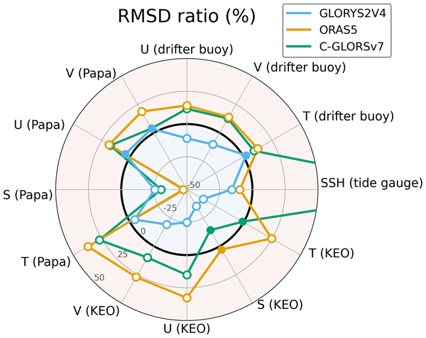
We developed an eddy-permitting EnKF-based ocean data assimilation system and produced the LETKF-based Ocean Research Analysis version 2.0 for a quasi-global domain (LORA-QG; Fig. 1) for the period from June 2002 to January 2024, during which the global ocean observing network was substantially enhanced by microwave satellite SST and Argo profiling float observations (Fig. 2). We compared the validation results among LORA-QG and three eddy-permitting global ocean reanalysis datasets (GLORYS2V4, ORAS5, and C-GLORSv7) using WOA18 (Figs. 3–6) and observations from surface drifter buoys (Figs. 7–11), tide gauges (Figs. 12 and 13), and ocean climate stations (KEO and Papa buoys; Figs. 14–18). LORA-QG, ORAS5, and C-GLORSv7 are independent of these observations, whereas GLORYS2V4 assimilates SST observations from the surface drifter buoys and temperature and salinity observations from the KEO and Papa buoys (Table 5). The validation results are summarized in a radar chart (Fig. 21), which shows RMSD ratios averaged over time and across space, stations, and depths for surface drifter buoys, tide gauges, and ocean climate stations, respectively. Although the ocean interior validation is limited to the KEO and Papa buoys, overall, the observations are best reproduced in the order of GLORYS2V4, LORA-QG, C-GLORSv7, and ORAS5. However, as discussed in Sects. 3.2 and 3.4.2, respectively, LORA-QG has significant warm biases in the tropics, especially in the western tropical Pacific, and it may not adequately reproduce SSS variations because relatively strong salinity nudging toward WOA18 is applied within the mixed layer.

Figure 21 Radar chart showing RMSD ratios of GLORYS2V4 (cyan), ORAS5 (orange), and C-GLORSv7 (green) averaged over time and across space, stations, and depths for the surface drifter buoys, tide gauges, and ocean climate stations, respectively. The bold black circle denotes a 0 % RMSD ratio, where the analysis RMSD is equal to that of LORA-QG; values outside and inside the circle indicate that LORA-QG reproduces the observations better and worse than the other datasets, respectively. Open circles indicate statistically significant differences from LORA-QG at the 99 % confidence level.

GLORYS2V4 and LORA-QG adopt the SEEK filter and the LETKF, respectively (Table 2); therefore, their forecast error covariance matrices vary in time. This characteristic may contribute to their higher accuracy compared with C-GLORSv7 and ORAS5. However, the ensemble spreads of LORA-QG are underdispersive for temperature, salinity, and horizontal currents at both the surface and in the ocean interior (Figs. 7e, 9e, 11a–c, 12e, and 15a–18a), although they are inflated through perturbations in atmospheric forcing and lateral boundary conditions and are maintained using RTPP. Consequently, some sources of model uncertainty remain insufficiently represented (e.g., uncertainties associated with vertical mixing and dissipation parameterizations), suggesting that additional stochastic perturbations or improved inflation techniques are needed to further increase the ensemble spread. Other parameters, such as the localization scale, may also require further tuning, but a detailed investigation of these aspects is beyond the scope of the present study.

Although the overall accuracy of LORA-QG is lower than that of GLORYS2V4, LORA-QG has important advantages, including ensemble-based uncertainty estimates and the availability of individual terms in the heat and salinity budget equations. The former is useful for improving prediction skill through ensemble forecasting, as demonstrated by Ohishi et al. (2025), while the latter facilitates the investigation of the mechanisms underlying temperature and salinity variations. The currently available period of LORA-QG spans from June 2002 to January 2024, reflecting the availability of microwave SST observations and the termination of the JRA55-do atmospheric forcing dataset in January 2024. Future work includes extending the system back to 1982, when infrared satellite SST observations became available, and developing a near-real-time system by incorporating AMSR3/GOSAT-GW SST assimilation (Fig. 2a) and replacing the atmospheric forcing with an available reanalysis dataset, such as ERA5 (Hersbach et al., 2020). We also developed a new eddy-resolving system and produced the LETKF-based Ocean Research Analysis version 2.0 for the North Pacific (LORA-NP; Fig. 2), covering the period since June 2002. We plan to validate LORA-NP and release both LORA-QG and LORA-NP through the JAXA-RIKEN Ocean Analysis website (https://www.eorc.jaxa.jp/ptree/LORA/index.html, last access: 10 September 2026).