An automated method for polynya detection using a geomorphon algorithm

Polynyas, persistent areas of open water within sea ice, are critical features of polar marine systems, facilitating ocean-atmosphere heat exchange, deep water formation, nutrient cycling, and biological productivity. However, current remote sensing approaches typically delineate polynyas using either sea ice concentration thresholds or thin sea ice thickness retrievals. While these methods have proven highly valuable, they can struggle to capture complex polynya morphology, especially fine-scale coastal features, and can be time-consuming to use and inconsistent across spatial scales. This study presents a novel application of a geomorphon pattern recognition algorithm, originally developed for terrestrial landform classification, to automate polynya detection using sea ice concentration data from the Advanced Microwave Scanning Radiometer 2 (AMSR2) ARTIST Sea Ice (ASI) product. Focusing on two key Southern Ocean regions, the Weddell and Amundsen Seas, we assess the algorithm's performance through a comprehensive sensitivity analysis involving multiple geomorphon parameter combinations and comparisons with traditional sea ice concentration threshold-based methods. By identifying morphological analogues, such as depressions and valleys in sea ice concentration data, the geomorphon method accurately captures polynya morphology, achieving F1-scores of 0.88–0.94 relative to threshold-based detections, while producing area estimates consistent with published observations. Additional sensitivity analyses examining both geomorphon parameter selection and uncertainty in the underlying sea ice concentration observations indicate that derived polynya areas are robust to plausible observational errors. The method's scalability and self-adaptive lookup distance allows detection of both large-scale open-ocean polynyas, and fine-scale coastal polynyas. The automated nature of the method enables efficient processing of large sea ice concentration data products while avoiding reliance on predefined concentration thresholds. Although further testing across additional regions, datasets, and polynya types is required, these results demonstrate that morphology-based classification provides a promising framework for automated and reproducible polynya detection and the generation of consistent long-term polynya records.

1 Introduction

1.1 Sea Ice and Polynya Dynamics

Sea ice is a defining feature of the polar regions and plays a large role in driving ocean circulation and global climate patterns by helping to regulate exchanges of heat, moisture, and salinity at the ocean-atmosphere boundary (Houghton et al., 1996). During sea ice formation, brine rejection increases the salinity and density of underlying surface waters, contributing to bottom water formation and global overturning circulation (Wakatsuchi and Ono, 1983; Comiso and Gordon, 1998; Nomura et al., 2021). Sea ice also provides a physical barrier between the relatively warm ocean and cold polar atmosphere, limiting heat and moisture exchange and influencing atmospheric circulation (Walsh and Johnson, 1979; Budikova, 2009; Landrum and Holland, 2022). Continuous sea ice can be interspersed with areas of open water, forming regions of direct interaction between the ocean and the atmosphere. These areas can be narrow linear fractures in sea ice, known as leads, or large semi-persistent openings, called polynyas. Polynyas are important oceanographic features, acting as sites of strong ocean-to-atmosphere heat and moisture exchange during the freezing season, which can modify local atmospheric and oceanic conditions (Alam and Curry, 1995; Gallée, 1997; Barber and Massom, 2007; Yager et al., 2016). They can also act as important carbon sinks through the sequestration of atmospheric CO₂ (Louanchi et al., 1999; Arrigo and van Dijken, 2003), with their collective influence potentially significant at broader spatial scales (Hoppema and Anderson, 2007).

Polynyas can range between 10 to 2–3 × 10⁵ km² in size and often occur at specific geographical locations and phases of the year (Morales Maqueda et al., 2004). Polynyas can be classified as either open-ocean or coastal and have different formation mechanisms (Gordon and Comiso, 1988). Open-ocean polynyas are typically thermally driven, occurring where warm buoyant water rises through the water column and melts sea ice (Martinson, 1991; Zheng et al., 2021). In contrast, coastal polynyas are typically formed when strong offshore winds advect sea ice away from the coast, creating areas of open water (Bromwich and Kurtz, 1984; Morales Maqueda et al., 2004; Bennett et al., 2024). These different formation processes mean that coastal and open-ocean polynyas can perform distinct physical and ecological roles. Open-ocean polynyas can act as sites of deep convection, influencing thermohaline circulation and facilitating nutrient upwelling (Melling et al., 2001; Cheon and Gordon, 2019). A prominent example is the Weddell Sea Polynya, which first gained scientific attention in the 1970s when it opened for several consecutive winters within the dense pack ice of the southern Weddell Sea (Carsey, 1980), with its re-emergence in the 2010s renewing scientific interest in its role in deep ocean convection (Mchedlishvili et al., 2022). By exposing relatively warm ocean to the atmosphere, the Weddell Sea Polynya promotes intense heat loss and vertical mixing, providing a rare window into processes that influence deep water formation and global thermohaline circulation (Cheon and Gordon, 2019). In comparison, coastal polynyas play important roles in local ice production, dense water formation, and high-latitude ecosystems (Comiso and Gordon, 1998; Kimura and Wakatsuchi, 2004; Arrigo and van Dijken, 2003). Increased open water and light availability during summer can support large phytoplankton blooms, making coastal polynyas important habitats for a range of benthic and higher trophic level organisms (Dennett et al., 2001; Jena and Pillai, 2020; Gilchrist and Robertson, 2000; Labrousse et al., 2018). Coastal polynyas in the Amundsen Sea are among the most biologically productive in the Southern Ocean, with the Amundsen Sea Polynya (ASP) and Pine Island Polynya (PIP) representing two of the largest and most persistent in the region (Arrigo and van Dijken, 2003). These polynyas have therefore become important sites for investigating links between sea ice variability, ocean circulation, and ecosystem dynamics (Arrigo and van Dijken, 2003; Arrigo et al., 2012).

The World Meteorological Organization (WMO) defines a polynya as a non-linear shaped opening enclosed within sea ice, which may contain open water, brash ice, new ice, nilas, or young ice (WMO, 2015). However, while this provides a general descriptive definition, operational criteria used to identify and delineate polynyas vary considerably between studies depending on the scientific objectives and data products employed. Most detection methods apply either sea ice concentration or thin sea ice thickness thresholds, which can vary widely depending on the application, to distinguish polynyas from the surrounding sea ice (Tamura and Ohshima, 2011; Ohshima et al., 2016; Mohrmann et al., 2021). Persistence criteria also differ, with some studies requiring openings to remain for certain periods before they are classified as polynyas (Arrigo and van Dijken, 2003). Size thresholds are rarely used, largely due to the spatial resolution constraints of available datasets. Furthermore, because coastal and open-ocean polynyas differ substantially in their morphology and formation mechanisms, the criteria adopted for delineation are often tailored to the specific research question. This diversity in operational definitions highlights the importance of clearly stating the criteria used when developing or applying a polynya detection technique.

1.2 Data Sources and Limitations

The ability to detect polynyas in observational satellite data and ocean reanalysis products is essential in improving our understanding of polynya dynamics. This is especially significant when we consider that their regionally and globally important roles are likely to be impacted by the effects of climate change, which will undoubtedly impact the extent and thickness of sea ice (Kim et al., 2023). Lack of in-situ data and observations of polynyas is often due to their remote locations in harsh environments, which make them challenging to access (Ohshima et al., 2016). Despite this, a range of different data sources have been employed to study polynyas, each with their own strengths and limitations, making them more suitable for some applications than others. Satellite remote sensing has been used in the majority of studies researching polynya inter-annual dynamics, monitoring sea ice concentration and thickness (Paul et al., 2015; Jena and Pillai, 2020). These products are particularly valuable for confirming the presence or absence of polynyas in specific regions and months and have supported many case studies of polynya variability (Zhou et al., 2023). However, even these technological advancements have limitations, including decreased performance during polar nighttime or with high cloud cover (Hall et al., 2004; Holz et al., 2008), which reduces their utility for long-term, consistent monitoring.

Passive microwave sensors are increasingly used for polynya detection because they can provide daily observations independent of cloud cover and time of day, allowing year-round monitoring of polar regions (Preußer et al., 2015; Jiang et al., 2020). As a result, passive microwave observations have become one of the most widely used data sources for investigating polynya variability across seasonal to multi-decadal timescales, through both sea ice concentration and thin sea ice thickness products (Tamura and Ohshima, 2011; Ohshima et al., 2016). Their consistent temporal coverage makes them particularly well suited for generating long-term records of polynya occurrence, extent, and persistence. Despite these advantages, passive microwave observations remain subject to several limitations. Their spatial resolution is often too coarse to fully resolve narrow coastal polynyas and complex coastline geometries, potentially leading to an underestimation of polynya extent (Barber and Massom, 2007; Burada et al., 2023). Derived sea ice concentrations can also be affected by land-spillover effects and mixed pixels near coastlines, where signals from land and sea ice become difficult to separate (Kern et al., 2022). In addition, uncertainties in the retrieval of thin sea ice can influence estimated sea ice concentrations within polynyas, while the application of fixed sea ice concentration or sea ice thickness thresholds can result in substantially different estimates of polynya area between studies (Massom et al., 1998; Kern et al., 2007; Mohrmann et al., 2021). For example, the extent and ice production of the North Water Polynya, the largest Arctic coastal polynya, has been shown to vary depending on the spatial resolution and characteristics of the satellite products used (Tamura and Ohshima, 2011; Iwamoto et al., 2014). Nevertheless, the broad spatial coverage, high temporal consistency, and long observational record provided by passive microwave products make them invaluable for investigating polynya dynamics. Their widespread use within the literature also provides a useful benchmark against which alternative polynya detection approaches can be evaluated.

1.3 Methods for Polynya Detection

Traditional methods of polynya detection generally rely on either sea ice concentration or thin sea ice thickness products, depending on the scientific application. Sea ice concentration methods are widely used to investigate polynya occurrence, extent and variability across Arctic and Antarctic regions (Massom et al., 1998; Monroe et al., 2021). However, no universally accepted threshold exists for the detection of all polynya types, with sea ice concentration thresholds commonly ranging from 0.2–0.8 depending on the sensor, retrieval algorithm, study region, time of year and associated sea ice conditions, and research objective (Massom et al., 1998; Mohrmann et al., 2021; Monroe et al., 2021). Consequently, estimates of polynya extent can vary substantially between studies. Thin sea ice thickness retrievals derived from passive microwave observations provide an alternative framework for identifying polynyas, particularly in studies concerned with sea ice production, ocean-atmosphere heat fluxes and dense water formation (Tamura and Ohshima, 2011; Nihashi and Ohshima, 2015; Ohshima et al., 2016). Rather than identifying open water using sea ice concentration thresholds, these approaches estimate thin ice thickness and use this information to calculate ice production and associated physical processes. As with sea ice concentration thresholds, the thickness criterion used to define thin ice is not standardised across studies. Thresholds of approximately 0.1–0.2 m are commonly adopted depending on the retrieval algorithm and scientific objective (Nakata et al., 2015; Ohshima et al., 2016), leading to differences in estimates of polynya extent, sea ice production and associated ocean-atmosphere heat exchange. In addition to threshold selection, many sea ice concentration and thickness detection frameworks require region-specific masking approaches and pre- and post-processing procedures to separate polynyas from neighbouring areas of open ocean and portions of the marginal ice zone (Fu et al., 2012; Nihashi and Ohshima, 2015). Furthermore, passive microwave observations are subject to uncertainties associated with mixed pixels, land-spillover effects, and thin-ice retrievals, which can influence the resulting polynya boundaries (Kern et al., 2022). These factors do not diminish the value of threshold-based approaches, but they do highlight the sensitivity of derived polynya extents to methodological choices and motivate the exploration of complementary detection frameworks that utilise additional spatial information beyond sea ice concentration thresholds alone.

While many polynya detection methods continue to rely on sea ice concentration thresholds, considerable effort has been devoted to automating these workflows and improving their reproducibility. For example, the Polynya Signature Simulation Method (PSSM) identifies open water, thin ice and thick ice using passive microwave polarisation ratios and brightness temperatures rather than derived sea ice concentration, but remains fundamentally a threshold-based classification framework (Markus and Burns, 1995; Kern et al., 2007; Kern, 2009). Similarly, recent studies have refined conventional threshold-based approaches to enable more automated detection of polynyas across large satellite datasets (e.g. Duffy et al., 2024; Lin et al., 2024). These developments demonstrate that threshold-based methods and automation are not mutually exclusive. Other approaches have sought to move beyond threshold-based classification altogether by exploiting additional spatial information or alternative data sources. Early image-processing techniques, including greyscale morphology methods (Fu et al., 2012), reduced some subjectivity in boundary delineation, while supervised and unsupervised classification of Sentinel-1 Synthetic Aperture Radar (SAR) imagery has improved the detection of small coastal polynyas (Burada et al., 2023). Similarly, Heuzé et al. (2021) used spaceborne infrared imagery to identify thermal precursors of Weddell Polynya openings, demonstrating how such observations can reveal atmospheric and oceanic preconditioning processes, although cloud cover and reduced temperature contrasts between sea ice and open water can limit their effectiveness. More recently, deep-learning frameworks have also been developed for automatic polynya identification (Heuzé and Wong, 2025; Landrum et al., 2026). For example, Heuzé and Wong (2025) introduced a deep-learning framework capable of automatic Arctic polynya detection, although its performance across long-term, multi-sensor datasets remains to be fully evaluated. Collectively, these studies demonstrate that automated polynya detection is already feasible across a range of observational datasets and methodological frameworks. However, differences in data requirements, parameter selection, training needs, and underlying assumptions can influence the resulting polynya classifications. This motivates continued exploration of alternative approaches, including morphology-based methods such as geomorphons, which utilise spatial patterns within sea ice concentration fields rather than predefined sea ice concentration or thin sea ice thickness thresholds alone.

Automated pattern recognition techniques, utilising algorithms and statistical methods, have long been used in terrestrial environments to classify topographic features into distinct landform types (e.g., Chorowicz et al., 1995; Jasiewicz and Stepinski, 2013). The “geomorphon” algorithm, developed by Jasiewicz and Stepinski (2013), classifies landforms based on local terrain morphology by analysing digital elevation models (DEM) and digital terrain models (DTM). Importantly, parameters within the algorithm can be customised to explore data at a range of spatial resolutions, meaning that the user can produce a landform map relevant to their specific study area and research question(s) (Jasiewicz and Stepinski, 2013; Wyles et al., 2022). Geomorphons have been used for various applications, including landform classification and mapping (Stepinski and Jasiewicz, 2011; Jasiewicz and Stepinski, 2013), predicting soil attributes (Flynn et al., 2020), and detecting treetops in complex forest structures (Antonello et al., 2017). More recently the method has been used with bathymetry data for marine ecological research, investigating the influence of seabed topographic features on the behaviour of shelf sea predators (Wyles et al., 2022). While initially developed for terrestrial geomorphology, the geomorphon algorithm is readily adaptable and therefore has potential applications within cryospheric research by treating variables such as sea ice concentration as analogous to elevation in topographic models. As with any approach based on sea ice concentration data, the resulting classifications remain dependent on the characteristics and uncertainties of the underlying observations, including potential biases associated with thin-ice retrievals and mixed-pixel effects near polynya boundaries. Nevertheless, because polynyas represent discontinuities within the surrounding sea ice cover, they may exhibit distinctive morphological signatures that can be identified using the geomorphon framework. To our knowledge, this approach has not previously been applied to polynya detection. Evaluating whether polynyas can be identified based on their morphology, rather than predefined sea ice concentration or thickness thresholds alone, represents an interesting opportunity to explore a complementary framework for automated polynya classification.

1.4 Study Objectives

The overall goal of this study is to evaluate the suitability of the geomorphon pattern recognition algorithm as an automated morphology-based framework for identifying polynyas from sea ice concentration data. By characterising polynyas according to their spatial morphology, rather than predefined sea ice concentration or thickness thresholds, the approach offers an opportunity to explore an alternative method for detecting both coastal and open-ocean polynyas. Improved and reproducible identification of polynyas and investigations into their variability has important consequences for several processes, such as ecosystem productivity and habitat availability (Gilchrist and Robertson, 2000; Arrigo and van Dijken, 2003; Arrigo et al., 2012; Labrousse et al., 2018), bottom water formation (Comiso and Gordon, 1998; Ohshima et al., 2016), and carbon sequestration (Hoppema and Anderson, 2007; Yager et al., 2016). The specific objectives of this paper are to: (i) evaluate the suitability of the geomorphon algorithm as a morphology-based framework for identifying coastal and open-ocean polynyas from sea ice concentration data; (ii) compare geomorphon-derived polynya extents with those obtained using conventional threshold-based approaches and with published estimates from the literature; (iii) assess the performance and consistency of the geomorphon approach across a range of seasonal sea ice conditions; and (iv) investigate the sensitivity of geomorphon-derived polynya extents to both algorithm parameter selection and uncertainty in the underlying sea ice concentration observations.

2 Data and Methods

2.1 Sea Ice Concentration Data

To evaluate the effectiveness and general applicability of a polynya detection method, both coastal and open-ocean polynyas must be considered, as they represent distinct classes of polynya with contrasting physical characteristics. The Amundsen Sea and Weddell Sea were selected as study regions because they represent contrasting polynya environments. The Amundsen Sea contains several recurrent coastal polynyas, whereas the Weddell Sea periodically hosts one of the largest open-ocean polynyas observed in the Southern Ocean (Morales Maqueda, 2004; Macdonald et al., 2023). Evaluating the geomorphon algorithm across both regions therefore provides an assessment of its ability to detect morphologically distinct polynya types. Sea ice concentration data for these two regions was obtained from the University of Bremen ASI (ARTIST Sea Ice) Version 5 sea ice concentration product derived from the Advanced Microwave Scanning Radiometer 2 (AMSR2) aboard the JAXA GCOM-W1 satellite (Spreen et al., 2008; Melsheimer and Spreen, 2019). The ASI algorithm retrieves sea ice concentration from passive microwave brightness temperatures measured at 89 GHz and provides daily gridded sea ice concentration fields at 6.25 km spatial resolution. Sea ice concentration is expressed as the fraction of each grid cell covered by sea ice, ranging from 0 (ice-free) to 1 (100 % ice cover). The product has been widely applied in sea ice and polynya studies owing to its relatively high spatial resolution, daily temporal coverage, and ability to provide observations independently of cloud cover and polar darkness. Daily sea ice concentration data from 2017 and 2020 were analysed for the Weddell Sea and Amundsen Sea respectively, as both years contained well-documented examples of their characteristic polynya types and allowed the geomorphon algorithm to be evaluated across a complete seasonal cycle encompassing polynya development, peak extent, decay, and periods of absence.

Daily sea ice concentration NetCDF files were downloaded from the University of Bremen archive and processed in R (Version 2024.12.1+563). The data was spatially subset to the study regions and reprojected to the Antarctic Polar Stereographic coordinate reference system (EPSG:3031) before being exported as GeoTIFF rasters for subsequent analysis (Fig. 1). The ASI Version 5 processing chain incorporates a land mask by excluding satellite footprints containing a non-zero land fraction and applying GMT5-based land masks and coastlines during gridding. Consequently, the coastline used in this study was inherited directly from the ASI product rather than generated independently. The ASI land mask was extracted and converted to a binary land-ocean raster for preprocessing, allowing coastlines to be preserved during geomorphon classification while excluding terrestrial cells from the analysis.

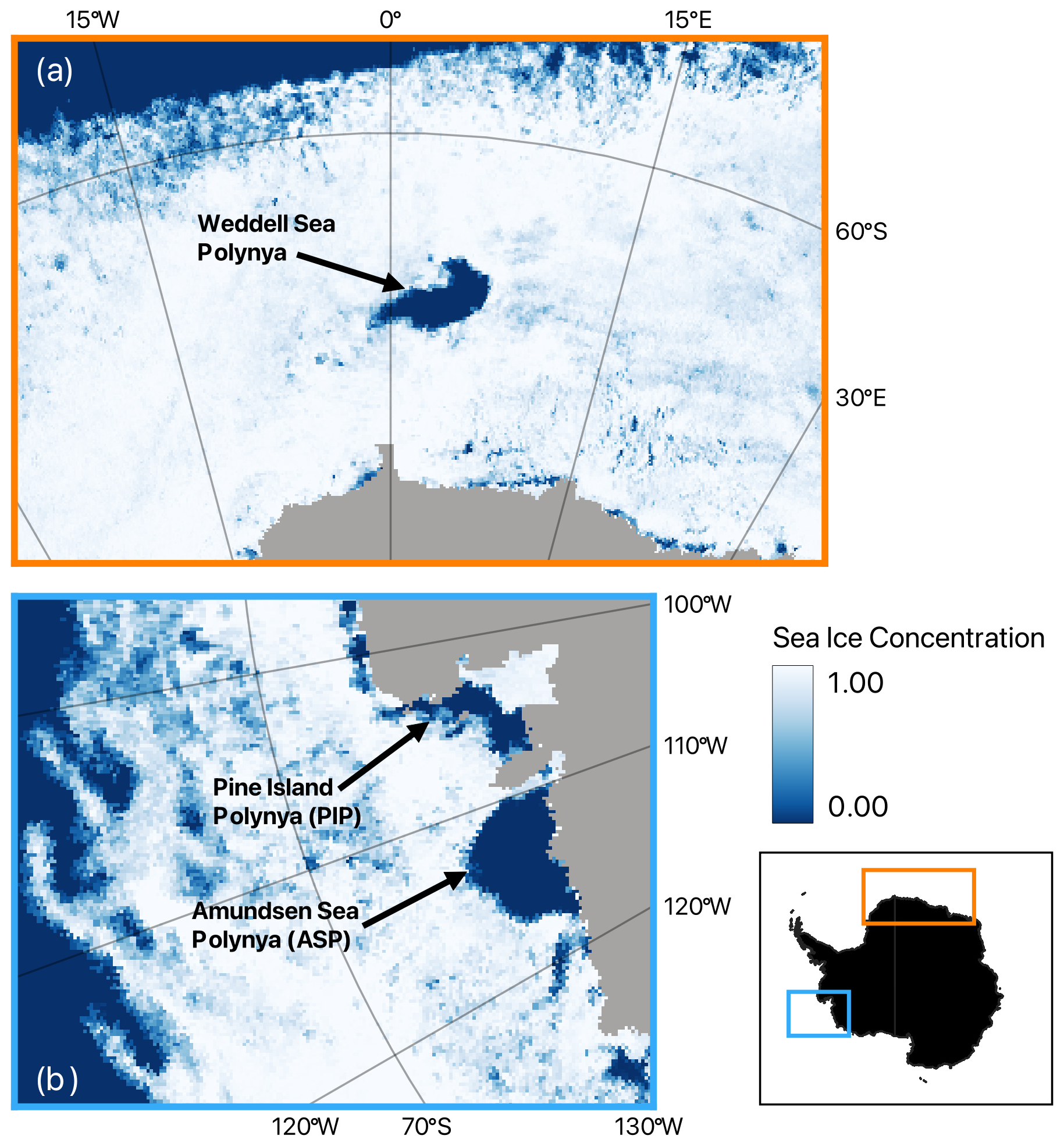
Figure 1 Daily sea ice concentration for the (a) Weddell Sea 15 October 2017, and (b) Amundsen Sea 15 December 2020. Insert shows the location of the Weddell Sea (orange) and Amundsen Sea (blue) on a larger scale. The Weddell Sea Polynya is labelled in (a), while the Amundsen Sea Polynya (ASP) and Pine Island Polynya (PIP) are labelled in (b). Daily data was obtained from the University of Bremen Archive, AMSR2 ASI sea ice concentration, version 5.4 (Melsheimer and Spreen, 2019).

2.2 Defining Polynyas for Detection

Due to the variation in definitions of polynyas discussed in the Introduction, we adopt a morphological definition in which a polynya is considered a distinct depression of low or absent sea ice embedded within the surrounding sea ice cover and isolated from the open ocean. This definition captures both coastal polynyas, where open water is bounded by continuous sea ice and a fixed coastal barrier (e.g., the coastline, land-fast sea ice, glacier fronts, or ice shelves), and open-ocean polynyas that are fully enclosed by continuous sea ice. No persistence or temporal duration criteria are applied, as the aim of this study is to evaluate the method's ability to detect polynyas rather than to analyse their temporal evolution. This morphological definition aligns directly with the geomorphon approach, which objectively identifies depressions based on spatial form rather than fixed sea ice concentration thresholds. At the same time, it remains compatible with traditional sea ice concentration threshold-based methods, as it identifies regions of reduced sea ice concentration that would typically fall below conventional cutoff values. As such, it provides a consistent framework for comparing the geomorphon-derived results with those obtained using sea ice concentration-based detection techniques.

2.3 Geomorphon Algorithm for Polynya Detection

Using DTM input data with a known spatial resolution (e.g., 250 m), the geomorphon pattern recognition algorithm produces a raster layer in which each grid cell is assigned one of the 10 most commonly recognisable landform elements associated with a terrestrial landscape (Fig. 2) (Jasiewicz and Stepinski, 2013). The algorithm requires the user to define three parameters which influence the classification of geomorphological features (Stepinski and Jasiewicz, 2011). The first is the search radius (search), which represents the maximum distance (m) from the central cell that the algorithm searches out from. The search parameter represents the maximum number of map cells over which the algorithm searches from the central cell. For example, for a DTM with a spatial resolution of 300 m, a search value of 10 corresponds to a maximum search radius of 3000 m. Rather than always using this full distance, the geomorphon algorithm determines the effective lookup distance for each cell automatically by identifying the local horizon in each search direction. Consequently, the user-defined search parameter acts as an upper limit, while the algorithm adapts the actual lookup distance to the surrounding topography (Stepinski and Jasiewicz, 2011). A relatively large search value should therefore be selected to encompass the maximum expected extent of a landform, allowing the algorithm to identify features across a range of spatial scales (e.g., narrow and wide valleys). If the search value is too small, landforms larger than the specified search radius may be fragmented into multiple landform elements. The second parameter, flatness threshold (flat), is the slope gradient (degrees) that is considered flat. Any gradient above this threshold is considered a deviation from a flat geomorphon and thus will represent one of the other 9 common landform elements. The third parameter is the spatial resolution of the DTM data, the value of which depends on what data source you are utilising. An additional optional parameter, flat distance (dist), can also be incorporated which defines the distance, measured in map cells, beyond which the algorithm gradually reduces the flat threshold. This prevents surfaces with a gradual slope from being misclassified as flat by accounting for elevation change which might occur over large distances. This is an important parameter to adjust when the spatial resolution of the user's DTM is low. The ability to adjust these parameters allows for the creation of a landform map that is specific to the user's spatial resolution and research question(s) of interest.

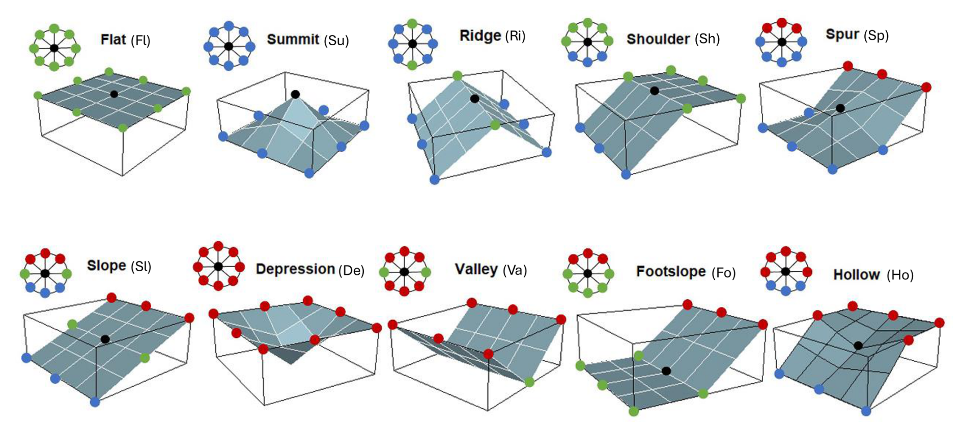
Figure 2 Symbolic 3D morphologies and their coordinating geomorphons (ternary patterns) for the 10 most common landform elements (adapted from Jasiewicz and Stepinski, 2013, and Wyles et al., 2022). Coloured points demonstrate if the cells surrounding the central cell (black) are lower (blue), higher (red), or the same elevation (green) as the central cell.

The geomorphon method utilises a line-of-sight principle for investigating the relationship of a central cell with its neighbouring cells in the DTM raster (Yokoyama et al., 2002). This means that the lookup distance is incrementally extended up to the predefined maximum value to determine the minimum zenith and nadir angles along eight compass directions from the central grid cell (Stepinski and Jasiewicz, 2011). These angles are then assessed to establish whether neighbouring cells are higher, lower, or the same elevation as the central cell. This classification is encoded into a ternary pattern which represents the geomorphon. Theoretically, there are 6561 possible topographic patterns, however, to reduce this for mapping they are condensed into the 10 most common landforms: flat, summit, ridge, shoulder, spur, slope, depression, valley, footslope, hollow (Fig. 2) (Jasiewicz and Stepinski, 2013). As a result, the output of the algorithm is a raster with values for each grid cell equivalent to one of these 10 landforms. Similar to changes in elevation seen in a DTM, variations in sea ice concentration across a body of water can produce unique spatial structures (Fig. 3). By applying the geomorphon algorithm to this data, it may be possible to determine polynyas from sea ice concentration structures that resemble certain classic landforms, such as valleys, depressions and hollows.

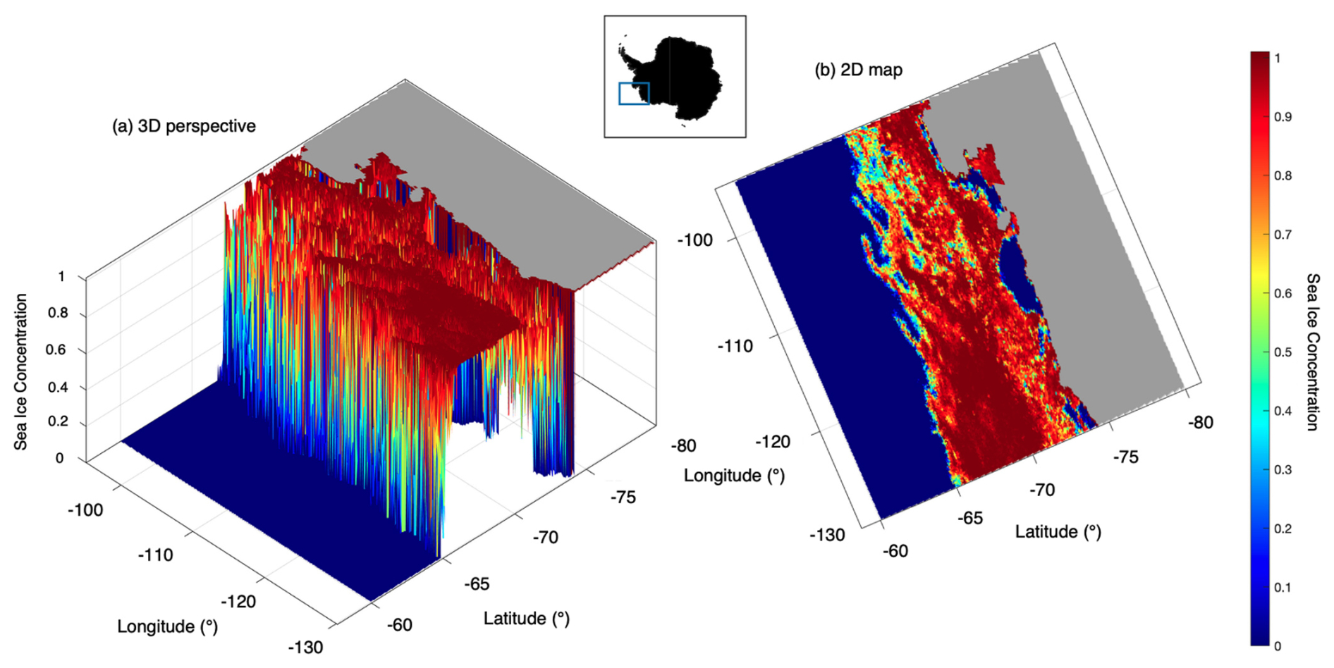
Figure 3 Example of daily sea ice concentration for the Amundsen Sea, 15 December 2020 (same as shown in Fig. 1b). (a) shows the three-dimensional perspective view of sea ice concentration, with (b) representing the two-dimensional map view of the same data. The dark blue steep declines in sea ice concentration seen near the coastline in (a) represent areas of coastal polynyas. Daily data was obtained from the University of Bremen Archive, AMSR2 ASI sea ice concentration, version 5.4 (Melsheimer and Spreen, 2019).

To ensure compatibility with the geomorphon algorithm, all sea ice concentration rasters were processed in the Antarctic Polar Stereographic coordinate reference system (EPSG:3031), as described in Sect. 2.1. This provided Cartesian coordinates in metres, allowing the geomorphon search and dist parameters to be specified directly as distance measures.

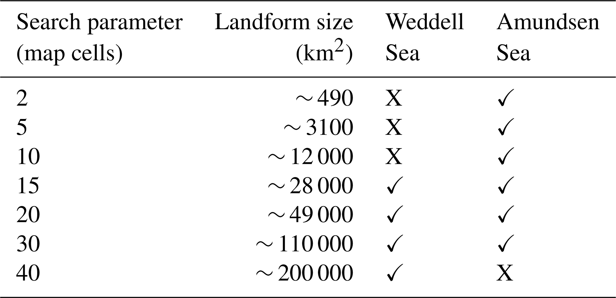
To determine the most suitable parameters for identifying polynyas from sea ice concentration data, a range of values for search, flat, and dist parameters were trialled with sea ice concentration data of a set spatial resolution (6250 m). The search parameter is measured in map cells and as a result requires knowledge of the spatial resolution of the sea ice concentration data and the size of the landform you are trying to classify to determine its value. A broad range of search values were tested, relating to varying search distances and resultant maximum landform sizes (Table 1). Smaller values were used for the Amundsen Sea, as coastal polynyas typically reach a smaller size than those which are open ocean (Mohrmann et al., 2021).

Table 1 Search parameter values used to test geomorphon algorithm on sea ice concentration data for the Amundsen and Weddell Seas. Each search distance corresponds to a maximum landform size (km²).

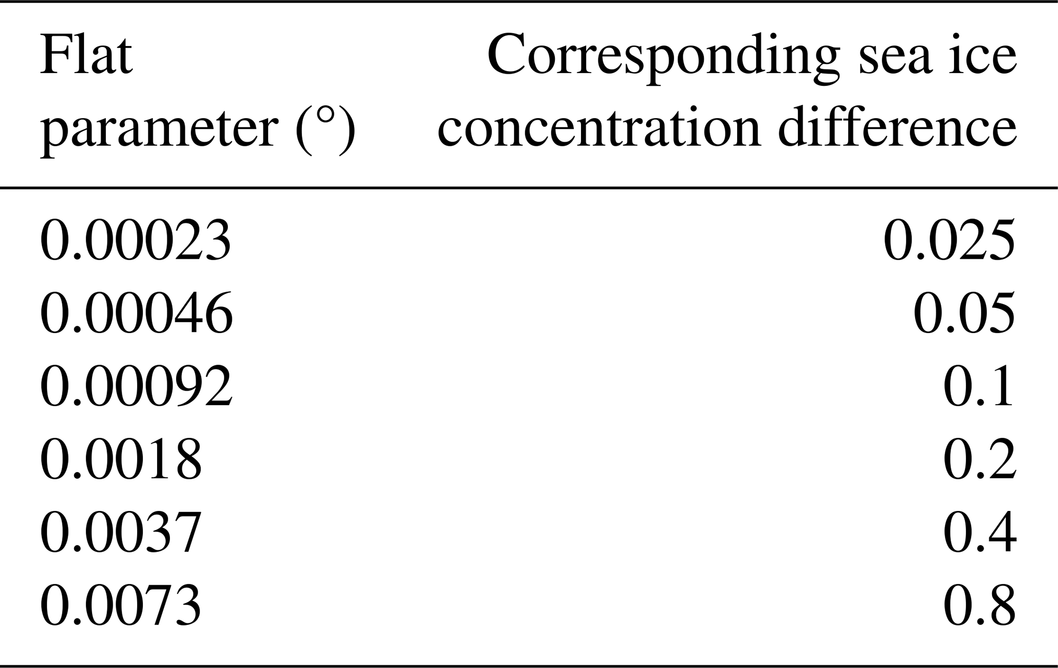
To adapt the geomorphon algorithm for sea ice concentration data, the flat parameter was reinterpreted in terms of sea ice concentration gradients. The spatial resolution of the data (6250 m) was used to convert differences in sea ice concentration between adjacent grid cells into slope angles. Specifically, the flat angle threshold (in degrees) was calculated using the inverse tangent function following Eq. (1):

$$\begin{array}{}\text{(1)}& \mathit{\theta }={\tan }^{-\mathrm{1}}\left({\displaystyle \frac{\mathrm{\Delta }\mathrm{SIC}}{d}}\right),\end{array}$$

where ΔSIC is the difference in sea ice concentration (SIC) between the central cell and its neighbours, and d is the horizontal distance between grid cells (6250 m). For example, a sea ice concentration difference of 0.4 corresponds to a slope angle of approximately 0.0037°, which is then used as the flat threshold value to classify any changes above this as “not flat”. A spectrum of flat parameter values was chosen to encompass a range of sea ice concentration thresholds which might be used for landform classification (Table 2). The same six values were used for both the Weddell and Amundsen Seas. Finally, four values of the dist parameter were evaluated (1.6, 3.2, 4.8 and 6.4 map cells), corresponding to approximately 10, 20, 30 and 40 km at the 6.25 km grid resolution of the AMSR2 ASI sea ice concentration dataset. These values were selected to represent a range of spatial scales over which gradual changes in sea ice concentration may occur and to assess the sensitivity of the geomorphon algorithm to the distance over which the flatness threshold is progressively relaxed. The same dist values were applied to both the Weddell and Amundsen Seas.

Having defined the parameter ranges and the spatial resolution of the sea ice concentration data, the Geographic Resources Analysis Support System (GRASS GIS) (Neteler and Mitasova, 2007) extension r.geomorphon (Jasiewicz and Stepinski, 2013) was implemented in R to classify geomorphons. All valid combinations of the search, flat, and dist parameters were evaluated. Parameter combinations in which dist exceeded search were excluded because the flat-distance parameter cannot be larger than the maximum search radius. Consequently, a total of 96 parameter combinations (4 search × 6 flat × 4 dist) were evaluated for the Weddell Sea, and whilst a total of 144 combinations were initially possible for the Amundsen Sea, 24 combinations occurred where dist > search and hence were invalid and omitted, resulting in 120 parameter combinations.

Table 2 Flat parameter values and their corresponding sea ice concentration differences between neighbouring grid cells used to test the geomorphon algorithm on sea ice concentration data for the Amundsen and Weddell Seas.

2.4 Threshold-Based Method for Polynya Detection

To provide a benchmark against which to evaluate the geomorphon approach, a conventional sea ice concentration threshold method was applied to the same daily AMSR2 ASI sea ice concentration data. Threshold-based classification remains the most widely used approach for detecting polynyas and therefore provides an appropriate reference for comparison with the morphology-based method developed in this study.

Grid cells with sea ice concentration ≤ 0.3 were initially classified as potential polynya pixels, while all remaining cells were classified as sea ice. The 0.3 threshold was selected because previous assessments have shown it provides a suitable balance between identifying polynyas and limiting false detections associated with higher or lower threshold values (Mohrmann et al., 2021). Higher thresholds tend to underestimate polynya extent by excluding regions of sparse sea ice, whereas lower thresholds increasingly classify embayments and marginal ice zones as polynyas (Mohrmann et al., 2021). Because a sea ice concentration threshold alone cannot distinguish enclosed polynyas from the adjacent open ocean, adjoining low-concentration regions connected to the open ocean were excluded by delineating enclosed polynya polygons within QGIS (version 3.42). This step ensured that only isolated regions satisfying the polynya definition adopted in Sect. 2.2 were retained for subsequent analysis. The resulting binary polynya masks (polynya = 1, non-polynya = 0) were then used as the reference dataset for evaluating the performance of the geomorphon algorithm. Although a 0.3 threshold was adopted for parameter optimisation and performance evaluation, additional analyses using 0.2, 0.6, and 0.8 thresholds were undertaken to illustrate the sensitivity of threshold-based polynya detection to the choice of sea ice concentration cutoff. These comparisons demonstrate the variability in estimated polynya extent arising solely from threshold selection, providing additional context for interpreting the geomorphon-derived results.

2.5 Parameter Tuning and Performance Evaluation

Initial parameter tuning was undertaken using two representative case studies selected from periods of well-documented polynya activity: 15 October 2017 for the Weddell Sea and 15 December 2020 for the Amundsen Sea (Fig. 1). These contrasting case studies were selected to provide representative examples of both open-ocean and coastal polynyas under favourable detection conditions, allowing the suitability of different geomorphon parameter combinations to be evaluated. For each study region, all valid combinations of the search, flat and dist parameters described in Sect. 2.3 were applied to the corresponding daily sea ice concentration raster. The resulting geomorphon classifications were converted to binary polynya maps by assigning cells classified as valleys, depressions, and hollows a value of 1 (polynya), with all remaining landform classes assigned a value of 0 (non-polynya). These binary classifications were then compared with the corresponding threshold-based reference dataset described in Sect. 2.4 using corresponding grid cells after both datasets had been resampled to a common analysis grid. The landforms valley, depression and hollow were chosen as these represent morphologies where the majority of neighbouring cells to the central cell are higher in elevation, thus closely mimicking a polynya, an area of low sea ice concentration surrounded by high sea ice concentration.

The performance of the geomorphon algorithm was evaluated using a confusion matrix comprising true positives (TP), false positives (FP), true negatives (TN), or false negatives (FN). From these quantities, precision, recall, and the F1-score were calculated:

$$\begin{array}{}\text{(2)}& {\displaystyle }\text{Precision}={\displaystyle \frac{\mathrm{TP}}{\mathrm{TP}+\mathrm{FP}}}\text{(3)}& {\displaystyle }\text{Recall}={\displaystyle \frac{\mathrm{TP}}{\mathrm{TP}+\mathrm{FN}}}\text{(4)}& {\displaystyle }\begin{array}{rl}\text{F1-Score}& =\mathrm{2}\times {\displaystyle \frac{\text{Precision}\times \text{Recall}}{\text{Precision}+\text{Recall}}}\\ & ={\displaystyle \frac{\mathrm{2}\times \mathrm{TP}}{\mathrm{2}\times \mathrm{TP}+\mathrm{FP}+\mathrm{FN}}}\end{array}\end{array}$$

Precision, recall, and F1-scores are commonly used evaluation metrics for classification tasks (e.g., Behera et al., 2019; Alem and Kumar, 2022). Precision measures the proportion of correctly identified polynyas among all detected polynyas, providing insight into how many of the identified features are actually true positives (Cook and Ramadas, 2020). Recall, on the other hand, assesses the proportion of polynyas identified by the threshold-based method that were correctly detected by the algorithm, indicating how well it captures actual polynya areas (Cook and Ramadas, 2020). The F1-score, which is the harmonic mean of precision and recall, balances these two metrics, ensuring that both false positives and false negatives are taken into account (Albaji et al., 2023). This combination of metrics allows for a comprehensive assessment of the algorithm's ability to accurately identify polynyas while minimising misclassification errors. To further validate the algorithm's effectiveness, visual and spatial comparisons were conducted for the best-performing parameter iterations, examining how well the detected landforms aligned with known polynya areas.

The best-performing parameter combination across both regions was determined by ranking the parameter combinations separately for each region based on their F1-score. The highest performing parameter combination for each region was used to re-run the geomorphon algorithm on a 12-month time series of daily sea ice concentration data, with the Weddell Sea analysed for 2017 and the Amundsen Sea for 2020. Polynya area across the time series was measured and compared with results from polynya area detected by the sea ice concentration threshold-based method.

2.6 Seasonal Consistency Assessment

Following the initial parameter tuning described in Sect. 2.5, the performance of the geomorphon algorithm was assessed across a complete annual cycle to evaluate its consistency under varying seasonal sea ice conditions. For each study region, the sea ice concentration raster corresponding to the 15th day of each month was selected, providing twelve representative daily scenes spanning the full range of seasonal conditions during 2017 for the Weddell Sea and 2020 for the Amundsen Sea. Using the 15th day of each month provided a consistent and evenly distributed temporal sample of seasonal sea ice conditions while avoiding preferential selection of particular polynya events. All valid combinations of the search, flat, and dist parameters were applied to each monthly scene and evaluated against the corresponding threshold-based reference dataset using the performance metrics described in Sect. 2.5. For scenes containing reference polynya pixels, parameter combinations were ranked according to their F1-score, allowing the consistency of classification performance to be assessed across periods of polynya development, peak extent and decay. For monthly scenes in which no reference polynya pixels were present, the F1-score is not informative because no true positive pixels exist. In these cases, parameter combinations were instead evaluated using the False Positive Rate (FPR):

$$\begin{array}{}\text{(5)}& \mathrm{FPR}={\displaystyle \frac{\mathrm{FP}}{\mathrm{FP}+\mathrm{TN}}}\end{array}$$

which quantifies the proportion of non-polynya pixels incorrectly classified as polynyas. This enabled algorithm performance to be assessed under ice-covered and open-water conditions by identifying parameter combinations that minimised false detections. The resulting seasonal performance distributions were used to identify parameter combinations that consistently performed well across contrasting sea ice conditions before proceeding to the sensitivity and uncertainty analyses.

2.7 Sensitivity and Uncertainty Analysis

2.7.1 Geomorphon Parameter Sensitivity

To quantify the sensitivity of geomorphon-derived polynya extent to parameter selection, five representative polynya conditions were identified for each study region using published literature describing characteristic polynya conditions together with visual interpretation of the daily sea ice concentration fields. These scenarios encompassed the range of sea ice conditions encountered throughout the annual cycle, including periods of polynya development, peak extent, decay and absence (Figs. A1 and A2). For the Amundsen Sea, an additional winter coastal polynya scenario was included to capture the persistence of coastal polynyas during the sea ice growth season, whereas for the Weddell Sea an open ocean absence scenario represented conditions following closure of the Weddell Sea polynya. For scenarios containing reference polynya pixels, parameter combinations were ranked according to their F1-score, and all combinations achieving at least 95 % of the maximum scene-specific F1-score were retained. This relative threshold retained parameter combinations exhibiting near-optimal classification performance while avoiding arbitrary selection based on negligible differences in skill. For scenarios in which no reference polynya pixels were present, parameter combinations were instead ranked using the FPR. Because F1-scores are undefined when no positive observations exist, all parameter combinations with a FPR within 0.001 of the minimum scene-specific value were retained. This ensured that parameter combinations with similarly low false detection rates were considered without imposing an arbitrary optimum. For each retained parameter combination, polynya area was calculated and the resulting range of area estimates was used to quantify the sensitivity of the geomorphon algorithm to parameter selection.

2.7.2 Sea Ice Concentration Uncertainty

To evaluate the influence of uncertainty in the underlying sea ice concentration observations, the uncertainty estimates provided in the University of Bremen AMSR2 ASI Version 5 product documentation were propagated through the geomorphon workflow. Rather than applying uncertainty directly to the calculated polynya area, uncertainty was incorporated into the input sea ice concentration fields prior to geomorphon classification, thereby accounting for the nonlinear response of the geomorphon algorithm to changes in the spatial structure of the sea ice concentration field. For each representative scenario, a concentration-dependent uncertainty raster was generated following the ASI product documentation, with uncertainties decreasing from approximately 25 % at 0 % sea ice concentration, to 10 % at 65 % sea ice concentration, and 5.7 % at 100 % sea ice concentration (Spreen et al., 2008; Melsheimer, 2024). Two deterministic perturbed sea ice concentration fields were then produced by subtracting and adding the corresponding uncertainty to each grid cell, with values constrained to the physically realistic range of 0 %–100 %. The geomorphon algorithm was subsequently applied to the original, lower-bound and upper-bound sea ice concentration fields using the final tuned parameter combination for each study region. Polynya area was calculated for each realisation, and the resulting minimum and maximum areas were used to define a deterministic sensitivity envelope representing the influence of sea ice concentration uncertainty on geomorphon-derived polynya extent.

3 Results

3.1 Performance of the Geomorphon Algorithm for Polynya Detection

To evaluate the suitability of the geomorphon algorithm as a morphology-based framework for identifying polynyas, parameter tuning was first undertaken by comparing geomorphon classifications with the corresponding 0.3 sea ice concentration threshold-based reference datasets for the Weddell Sea (15 October 2017) and Amundsen Sea (15 December 2020). Across all tested parameter combinations, we examined the most frequently assigned geomorphon landforms at areas classified as polynyas and non-polynyas by the threshold-based method (Fig. B1). The four most common geomorphon landforms associated with polynyas were the same across both the Amundsen and Weddell Sea, being flat (39.5 %, 34.4 %), footslope (29.0 %, 35.7 %), hollow (17.1 %, 14.9 %), and depression (1.2 %, 2.0 %). For non-polynya regions (i.e., areas of open ocean or sea ice concentration > 0.3), flat landforms were the most common for both the Amundsen (80.0 %) and Weddell (71.9 %) Seas. In the Weddell Sea, shoulder (6.5 %) and ridge (5.9 %) landforms were also commonly associated with non-polynya areas. Nearly identical proportions were observed in the Amundsen Sea, with shoulder (6.5 %) and ridge (5.7 %) landforms similarly classified as non-polynya.

There was considerable variability in precision and recall scores across parameter combinations (Fig. C1). Across all parameter combinations, the algorithm achieved higher average precision in the Amundsen Sea (0.42) than in the Weddell Sea (0.23), whereas average recall was greater in the Weddell Sea (0.53) compared to the Amundsen Sea (0.47). The broader spread in precision-recall scores observed for the Amundsen Sea reflects the greater variation in search radius values used during algorithm iterations. Examining precision and recall by specific parameter values reveals that higher search values (> 15 map cells) yield higher precision and recall scores in both the Amundsen and Weddell regions (Fig. C2). Increasing the flat threshold produced progressively higher precision but lower recall, with precision peaking at a flat threshold of 0.0037° before declining sharply at 0.0073° in both regions. In contrast, varying the dist parameter had relatively little influence on precision or recall for either region.

Given the variability in precision and recall, F1-scores also exhibited considerable variation across both regions, with certain parameter combinations yielding notably higher classification success than others (Figs. 4 and 5). For the Weddell Sea October 2017, the highest F1-scores (> 0.7) were achieved by iterations of the algorithm which included flat thresholds of 0.0018° and 0.0037° (Fig. 4). The lower flat thresholds achieved a higher F1-score when combined with a higher dist parameter value, whilst the higher flat values attained higher F1-scores when paired with lower dist values. The highest F1-scores were also seen when the search distance parameter had values of 30 and 40 map cells. The same general pattern is observed for the Amundsen Sea December 2020, whereby flat thresholds of 0.00092°, 0.0018°, or 0.0037° achieved the highest F1-scores (> 0.7), with the lower dist parameter values attaining higher F1-scores when paired with higher flat thresholds and vice versa (Fig. 5). Higher values of the search parameter also yielded the highest F1-scores, with 20 and 30 map cells performing the best.

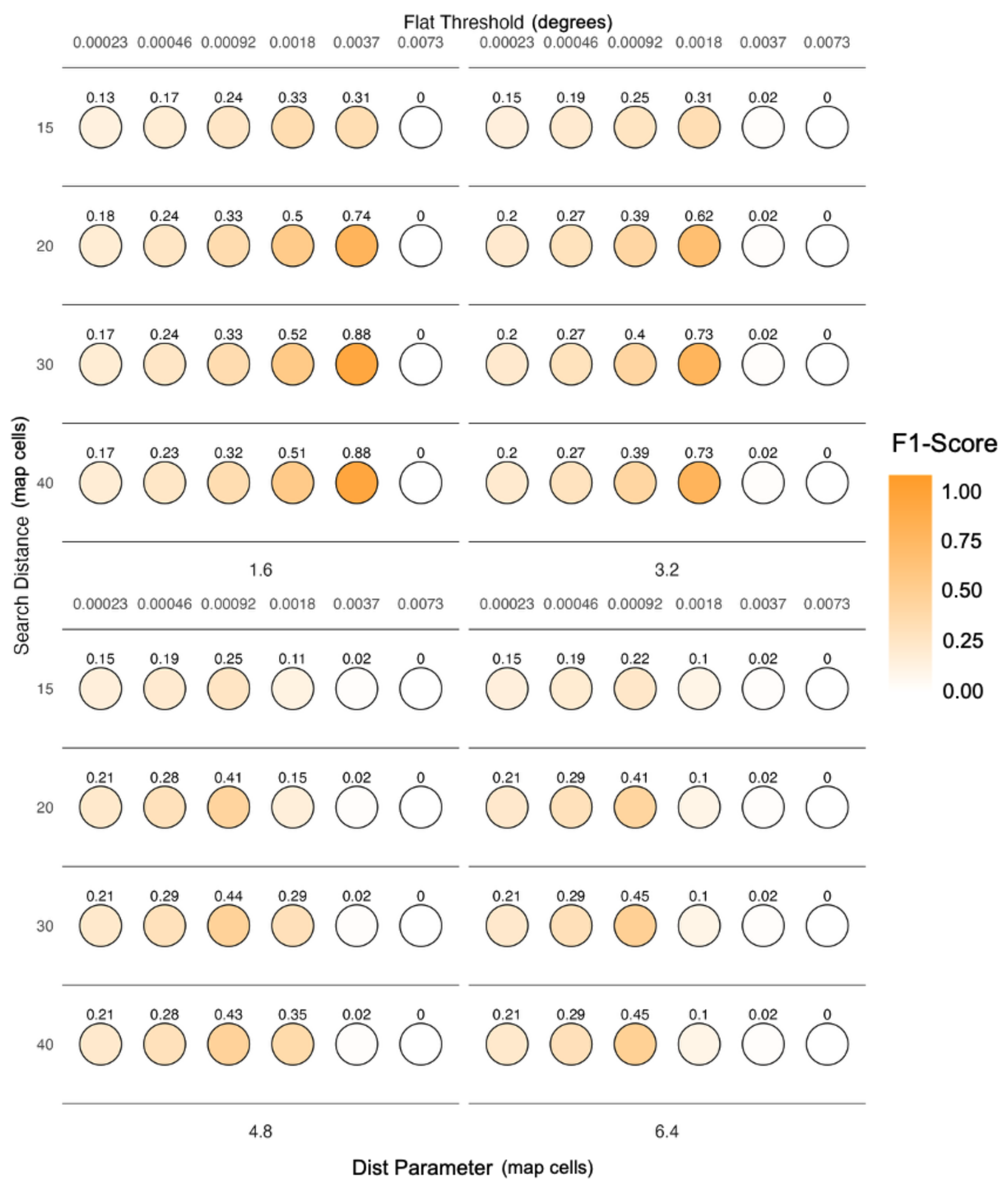
Figure 4 F1-scores for all tested parameter combinations of the geomorphon algorithm for the Weddell Sea. Each dot represents a unique combination of search, flat, and dist parameters, with shading corresponding to F1-score. Higher F1-scores indicate better agreement between geomorphon classifications and polynya areas defined by the 0.3 sea ice concentration threshold-based method.

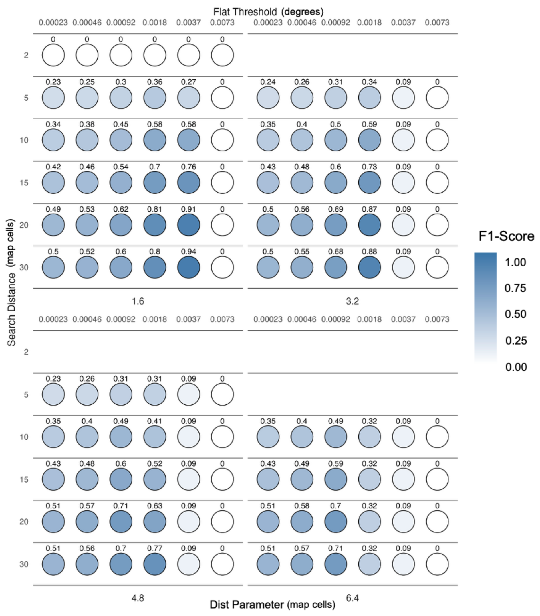
Figure 5 F1-scores for all tested parameter combinations of the geomorphon algorithm for the Amundsen Sea. Each dot represents a unique combination of search, flat, and dist parameters, with shading corresponding to F1-score. Higher F1-scores indicate better agreement between geomorphon classifications and polynya areas defined by the 0.3 sea ice concentration threshold-based method.

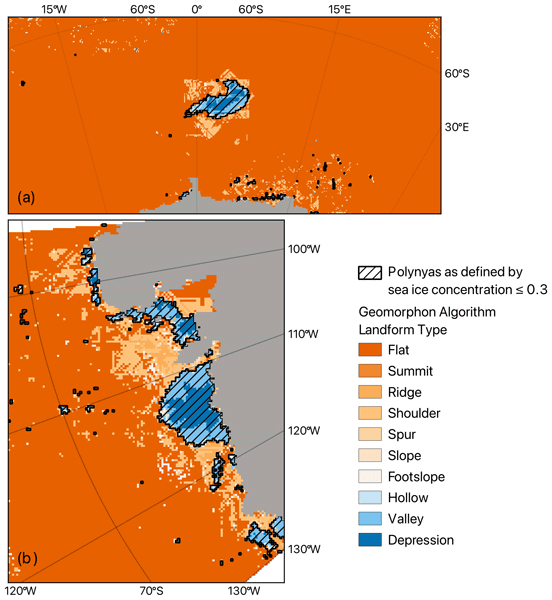
The best performing combination of parameter values in the Weddell Sea achieved an F1-score of 0.88 and included a flat threshold of 0.0037°, search distance of 40 map cells, and dist parameter of 1.6. For the Amundsen Sea, the best performing parameter combination achieved an F1-score of 0.94 with a flat threshold of 0.0037°, search distance of 30 map cells, and dist parameter of 1.6. When compared visually with the polynyas identified using the sea ice concentration threshold (≤ 0.3) method, the geomorphon-detected polynya identifying landforms produced by these parameter sets, show strong spatial agreement, as valleys, depressions and hollows align closely with polynya areas defined by the threshold-based method (Fig. 6).

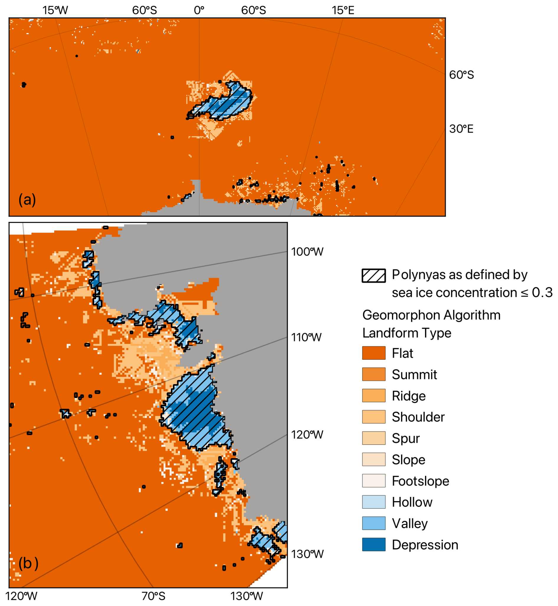
Figure 6 Geomorphon landform classifications for the representative parameter tuning case studies in the (a) Weddell Sea (15 October 2017) and (b) Amundsen Sea (15 December 2020). The best-performing parameter combinations were used for each region respectively, with flat = 0.0037°, search = 40 map cells, dist = 1.6 map cells used for the Weddell Sea classification, and flat = 0.0037°, search = 30 map cells, and dist = 1.6 map cells used for the Amundsen Sea classification. Areas identified as polynyas using the sea ice concentration threshold (≤ 0.3) are outlined in black hatching. Geomorphon landforms associated with polynya detection (hollow, depression and valley) are shown in shades of blue, whereas the remaining landform classes are shown in shades of orange.

3.2 Seasonal Consistency Across Sea Ice Conditions

To assess the seasonal consistency of the geomorphon algorithm, all valid parameter combinations were evaluated using representative daily sea ice concentration scenes from the 15th of each month in 2017 (Weddell Sea) and 2020 (Amundsen Sea; Appendix D). For monthly scenes containing one or more reference polynya pixels, performance was evaluated using the F1-score, whereas monthly scenes without reference polynya pixels were evaluated using the FPR. Across both study regions, the flat threshold exhibited the greatest consistency throughout the annual cycle, with the highest F1-scores generally occurring at or near 0.0037°. In contrast, the search parameter producing the highest F1-score varied between months, although larger search values (20–40 map cells) most frequently achieved the highest performance. Changes in the dist parameter had comparatively little effect on F1-scores across the majority of monthly scenes. For months in which no reference polynya pixels were present, performance was assessed using the FPR, the same general parameter patterns were observed. Lower FPR values were consistently associated with larger search values, flat thresholds close to 0.0037°, and comparatively small differences between dist parameter values.

3.3 Polynya Area Estimates Using the Geomorphon Algorithm

Daily polynya area estimates derived using the final geomorphon parameter combinations are shown alongside those obtained using the ≤ 0.3 sea ice concentration threshold method for the Amundsen and Weddell Seas (Fig. 7). In both regions, the geomorphon algorithm reproduced the seasonal evolution of polynya extent, with periods of polynya formation, maximum extent and decay occurring at similar times to those identified by the threshold-based approach. In the Amundsen Sea, the largest polynya extents occurred during the austral summer months (January–March), followed by a marked reduction in area during autumn and winter before increasing again towards the end of the year (December) (Fig. 7). In the Weddell Sea, polynya activity was concentrated between June and November, with the largest extents observed during November before decreasing rapidly during December (Fig. 7). Monthly maxima occurred during January in the Amundsen Sea and November in the Weddell Sea for both the geomorphon and threshold-based methods. Throughout the annual cycle, geomorphon-derived area estimates were generally lower than those obtained using the threshold-based method. The maximum geomorphon-derived area was approximately 95 000 km² in the Amundsen Sea and 90 000 km² in the Weddell Sea.

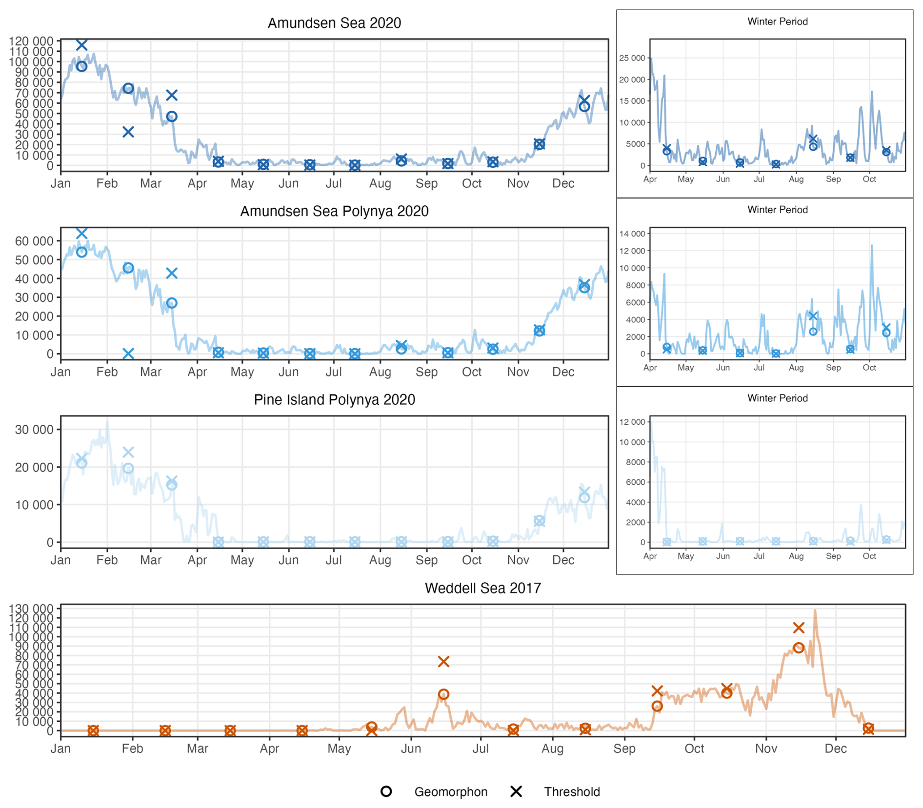
Figure 7 Polynya area estimates for the whole Amundsen Sea, Amundsen Sea Polynya, and Pine Island Polynya (2020). Pale solid lines show the complete daily geomorphon-derived polynya area time series using the final parameter combinations (Amundsen Sea: flat = 0.0037°, search = 30 map cells, dist = 1.6 map cells; Weddell Sea: flat = 0.0037°, search = 40 map cells, dist = 1.6 map cells). Open circles indicate the geomorphon-derived polynya area for the daily sea ice concentration field corresponding to the 15th day of each month used in the seasonal consistency assessment; these symbols represent individual daily estimates rather than monthly mean values. Crosses indicate the corresponding daily polynya area estimates derived using the ≤ 0.3 sea ice concentration threshold method for the same dates. Insets show the April-October period using an expanded y-axis to highlight the smaller winter polynya areas in the Amundsen Sea.

Within the Amundsen Sea, both the ASP and PIP exhibited similar seasonal patterns, with maximum extents occurring during January–March, very low polynya area between May and October, and redevelopment during November and December (Fig. 7). Throughout the annual cycle, geomorphon-derived area estimates closely followed those obtained using the threshold-based method for both polynyas, although the geomorphon estimates were generally smaller. Maximum geomorphon-derived areas of approximately 54 000 and 21 000 km² were observed for the ASP and PIP, respectively. The greatest difference between the two approaches was observed in February for the ASP. The geomorphon algorithm estimated an area of approximately 45 000 km², whereas the threshold-based method identified only approximately 100 km² (see Discussion, Sect. 4.2).

3.4 Sensitivity to Geomorphon Parameter Selection and Sea Ice Concentration Data Uncertainty

To investigate the sensitivity of geomorphon-derived polynya extents to algorithm parameter selection, parameter combinations achieving comparable classification performance were retained for each representative scenario (Figs. A1 and A2). For scenarios containing one or more reference polynya pixels, parameter combinations achieving at least 95 % of the maximum F1-score were retained, whereas scenarios without reference polynyas retained parameter combinations within 0.001 of the minimum FPR. The best-performing parameter combination identified for each region during the tuning process satisfied the F1-score or FPR retention criteria for all representative scenarios except one (Fig. E1). The only exception was the Amundsen Sea July 2020 frozen-over or absent polynya scenario, for which the best tuning process parameter combination did not meet the retention criterion. Nevertheless, this parameter combination was retained for the subsequent uncertainty analysis to enable the performance and resulting uncertainty of the final parameter set to be evaluated consistently across the full range of seasonal sea ice conditions and polynya states. Between 2 and 16 parameter combinations were retained across the Amundsen Sea scenarios, compared with between 2 and 75 combinations for the Weddell Sea scenarios. Among the retained parameter combinations, retained F1-scores for the Amundsen Sea ranged from 0.71 to 0.96. The only exception was the manually retained parameter combination for the July 2020 frozen-over or absent polynya scenario, which achieved an F1-score of 0.34 and therefore fell outside this range. For the Weddell Sea, retained parameter combinations produced F1-scores ranging from 0.69 to 0.93, while FPRs ranged from 0 to 0.00098.

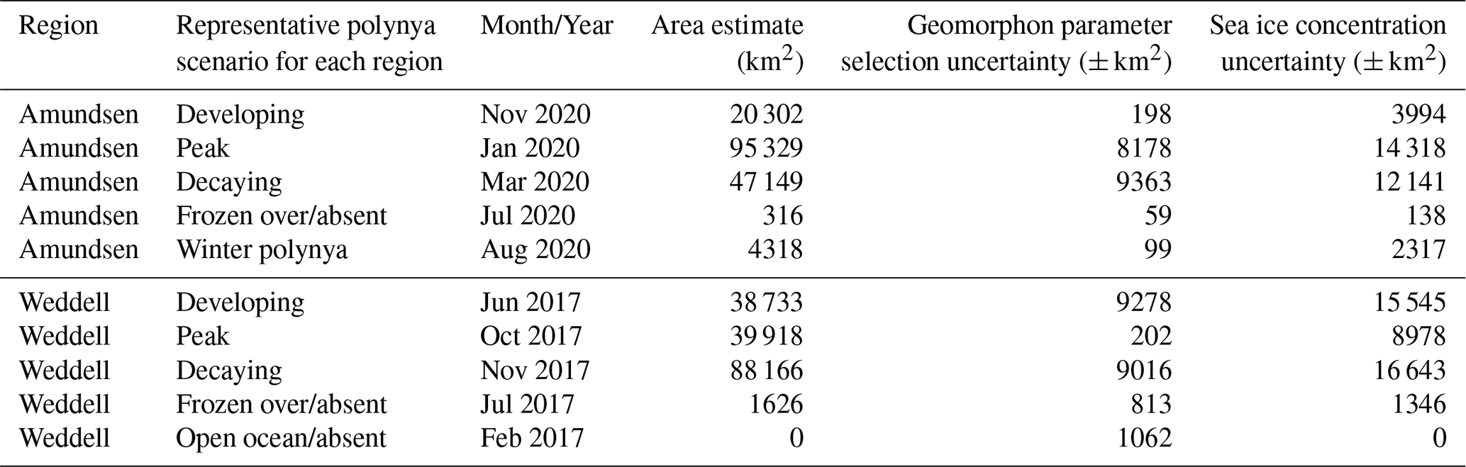
The retained parameter combinations were subsequently used to quantify the sensitivity of geomorphon-derived polynya area estimates to algorithm parameter selection and to compare this source of uncertainty with that arising from uncertainty in the underlying sea ice concentration observations (Table 3). Across the representative scenarios, geomorphon parameter uncertainty ranged from ±59 to ±9363 km² in the Amundsen Sea and from ±202 to ±9278 km² in the Weddell Sea (Table 3). Perturbing the sea ice concentration fields using the uncertainty estimates provided in the AMSR2 ASI Version 5 product documentation resulted in uncertainties ranging from ±138 to ±14 318 km² in the Amundsen Sea and from 0 to ±16 643 km² in the Weddell Sea. For the developing, peak and decaying polynya scenarios in both regions, uncertainty associated with the sea ice concentration data exceeded that arising from geomorphon parameter selection. In contrast, the frozen-over/absent and open-ocean absent scenarios exhibited comparable or larger uncertainties associated with parameter selection.

Table 3 Geomorphon-derived polynya area estimates and associated uncertainty for the region-specific representative polynya scenarios. Area estimates correspond to the final parameter combination selected for each region. Geomorphon parameter uncertainty (± km²) was calculated as half of the range between the minimum and maximum polynya areas obtained from all retained parameter combinations, while sea ice concentration data uncertainty (± km²) was derived by perturbing the input ASI AMSR2 sea ice concentration fields using the uncertainty estimates reported in the product documentation.

4 Discussion

This study evaluated the potential of the geomorphon pattern recognition algorithm as a morphology-based framework for automated polynya detection from passive microwave sea ice concentration data. By assessing performance across two contrasting Southern Ocean polynya systems, multiple seasonal conditions, and a range of geomorphon parameter combinations, this study provides the first comprehensive evaluation of the approach for both coastal and open-ocean polynyas. Overall, the geomorphon algorithm consistently identified polynya extent with strong agreement to conventional threshold-based methods while remaining robust to variations in parameter selection and sea ice concentration uncertainty. These findings suggest that morphology-based classification provides a promising complementary framework for objective and reproducible polynya detection. The following sections discuss the performance of the approach, its relationship to existing detection methods, its robustness and limitations, and its potential application to long-term monitoring.

4.1 Geomorphons as a Morphology-Based Framework for Polynya Detection

The geomorphon analysis identified clear differences in the distribution of landform classes between polynya and non-polynya regions, supporting the concept that distinct spatial morphologies within sea ice concentration fields can be used to identify polynyas. Depressions, hollows and valleys were consistently associated with polynya regions, reflecting their ability to capture localised minima in sea ice concentration relative to the surrounding pack ice. In contrast, flat landforms dominated non-polynya areas, representing regions of relatively homogeneous sea ice concentration, while shoulders, ridges and spurs occurred more frequently within consolidated pack ice where stronger structural gradients exist (Comiso et al., 2003; Andersen et al., 2007). These associations are consistent with the expected morphology of polynyas as localised breaks within an otherwise continuous sea ice cover, providing support for the application of morphology-based classification to sea ice concentration data.

Some overlap between geomorphon landform classes in polynya and non-polynya regions highlights that individual landforms cannot be used in isolation to identify polynyas. For example, footslopes occurred frequently within polynya regions across many parameter combinations, but in the highest-performing configurations features were primarily concentrated along the boundary between the open-water region of the polynya and the surrounding higher sea ice concentrations (Fig. 6). This distribution is consistent with the geomorphon definition of footslopes as transitional landforms between lower and higher elevations (Fig. 2), analogous to the strong sea ice concentration gradient that occurs between a polynya and the surrounding pack ice (Worby and Comiso, 2004; Bitz et al., 2005). In contrast, depressions, hollows and valleys were more consistently associated with the interior of polynyas, where sea ice concentrations are lower than the surrounding pack ice. These findings indicate that successful polynya detection depends not on a single geomorphon class, but on selecting the combination of landforms that best represents the characteristic morphology of polynyas while excluding landforms commonly associated with surrounding sea ice or open ocean.

This study focused on evaluating the ability of the geomorphon framework to detect polynyas rather than providing a detailed physical interpretation of every geomorphon landform class within sea ice concentration fields. A more comprehensive investigation of how individual geomorphon classes relate to specific sea ice structures, including leads, ridges, marginal ice zones and newly formed sea ice, would improve understanding of the physical basis of the classifications and represents an important direction for future research. Such work may also reveal broader applications of geomorphons for characterising sea ice morphology beyond polynya detection alone.

4.2 Comparison with Threshold-Based Method and Published Polynya Extents

Performance metrics revealed substantial variation across the 120 and 96 parameter combinations tested for the Amundsen and Weddell Seas respectively, highlighting the importance of tuning the algorithm to the scale and context of polynya identification. Overall, the best-performing iterations of the algorithm included the largest search distance tested for each region, of 30 and 40 map cells, and slightly higher flat threshold of 0.0037°, combined with the lowest dist parameter value (Fig. 6). In the context of the AMSR2 ASI sea ice concentration data, these parameter values translate to a search radius of 187.5–250 km, which equates to a maximum polynya area of ∼ 110 000–200 000 km², and a sea ice concentration threshold of 0.4 (Tables 1 and 2). These values are consistent with the known oceanographic characteristics of polynyas, as they typically range in size from 10 to 10⁵ km² (Morales Maqueda et al., 2004). Moreover, sea ice concentration within polynyas varies considerably, especially in coastal polynyas which are sites of vast sea ice production (Tamura and Ohshima, 2011; Zhou et al., 2023). As a result, the best-performing flat threshold corresponding to a moderate sea ice concentration threshold is understandable, as polynyas are not always homogenous areas of open water surrounded by high sea ice concentration (Kwok et al., 2007; Gutjahr et al., 2016).

Comparison of the geomorphon-derived and ≤ 0.3 sea ice concentration threshold-based polynya areas demonstrates that both methods capture the overall seasonal evolution of polynya extent across the Amundsen and Weddell Seas (Fig. 7). In both regions, the timing of polynya expansion and contraction is highly consistent, with peak extents occurring during austral summer in the Amundsen Sea and during the well-documented opening of the Weddell Sea Polynya in late 2017. This consistency indicates that the geomorphon framework successfully reproduces the major temporal characteristics of polynya development despite relying on a fundamentally different detection principle. Differences between the approaches are primarily observed in the estimated magnitude of polynya area rather than the timing of polynya occurrence. In the Amundsen Sea, the geomorphon method generally identified larger polynya extents than the 0.3 threshold during the summer months, whereas the similarity between the two approaches was considerably closer during winter when polynyas were small or absent. In contrast, both methods produced more similar estimates for the Weddell Sea throughout much of the 2017 event, although differences remained during periods of rapid polynya expansion and contraction. These discrepancies most likely reflect the differing principles of the two detection methods. Whereas threshold-based approaches classify all grid cells below a predefined sea ice concentration as polynyas, the geomorphon algorithm identifies local morphological depressions within the sea ice concentration field, allowing the detected boundary to respond to spatial gradients rather than a single concentration value.

These differences highlight the influence that the choice of detection methodology can have on estimated polynya extent. To investigate this further, geomorphon-derived areas were compared with polynyas identified using a range of commonly applied sea ice concentration thresholds. Figure 8 demonstrates that estimated polynya extent is highly sensitive to the sea ice concentration threshold selected. Across both study regions, progressively higher thresholds produced systematically larger estimates of polynya area, with the greatest divergence occurring during periods of polynya growth and peak development. This highlights the influence that threshold selection alone can have on reported polynya extents and reinforces the difficulty of applying a single sea ice concentration threshold consistently across different seasons and regions. The relationship between the geomorphon-derived estimates and the threshold-based approaches also varied seasonally. During winter and spring, when polynyas were small or developing, the geomorphon-derived areas generally fell within the range defined by the four threshold methods, often lying between the lower (0.2–0.3) and higher (0.6–0.8) sea ice concentration thresholds. This suggests that the morphology-based approach identifies polynya extents that are consistent with conventional threshold methods without relying on a predefined concentration value. In contrast, during the summer months the geomorphon method generally produced smaller area estimates than all four threshold approaches, before returning towards the threshold-derived range during autumn as polynyas contracted. It should also be recognised that comparisons between methods become increasingly difficult during late spring and summer as the surrounding sea ice cover becomes less consolidated. Under these conditions, a fixed sea ice concentration threshold may delineate regions of relatively lower sea ice concentration rather than a clearly defined opening within compact sea ice, making the definition of a polynya progressively less distinct.

A notable exception occurred for the ASP during February, where the geomorphon-derived area remained substantially larger than the threshold-based estimate (Figs. 7 and 8). Investigation of the spatial comparison shows that this difference arose because the threshold-based method classified the polynya as connected to the open ocean and therefore excluded it from the analysis, whereas the geomorphon algorithm continued to identify it as a distinct enclosed feature. Examination of the sea ice concentration contours suggests that, although the surrounding sea ice concentration gradients continued to define a distinct enclosed depression, the low sea ice concentration region was no longer completely separated from the adjacent open ocean when a fixed ≤ 0.3 sea ice concentration threshold was applied. Consequently, the threshold-based approach treated the polynya and adjacent open ocean as a single connected feature, whereas the geomorphon algorithm continued to identify the enclosed morphological depression as a distinct polynya (Fig. F1). Although this behaviour may represent an advantage of the morphology-based approach during transitional states, additional evaluation using higher-resolution observations would be valuable to determine which representation more accurately reflects the physical structure of the polynya.

The summer underestimation likely reflects differences in how the two approaches define polynya boundaries. During peak summer, coastal polynyas often exhibit less distinct boundaries, with gradual transitions between open water, thin or unconsolidated ice, and the surrounding pack ice as sea-ice concentrations decrease (Wei et al., 2021; Lin et al., 2024). Threshold-based methods progressively include these transitional regions as higher sea ice concentration thresholds are applied, whereas the geomorphon algorithm identifies the core morphological depression within the sea ice concentration field. Consequently, the geomorphon-derived boundary remains comparatively conservative during periods of maximum polynya extent. Although threshold-based approaches require the selection of a single sea ice concentration value, no universally accepted threshold exists for polynya detection, with values between 0.2 and 0.8 commonly used depending on the study region, season and research objective (Massom et al., 1998; Mohrmann et al., 2021). The geomorphon framework instead identifies polynyas from the spatial morphology of the sea ice concentration field, avoiding direct classification based on a single sea ice concentration threshold while producing area estimates comparable to those obtained using a range of threshold values.

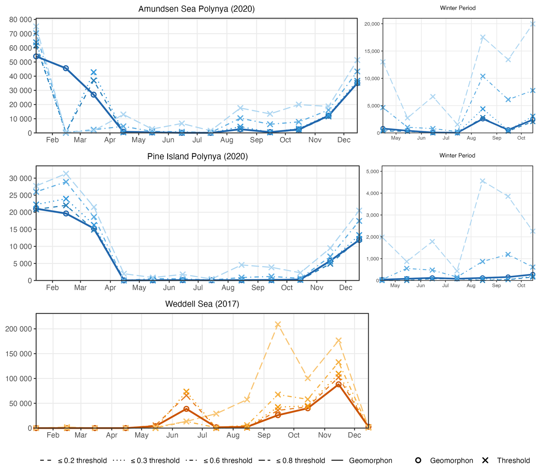
Figure 8 Polynya area estimates for the Amundsen Sea Polynya and Pine Island Polynya in 2020 and the Weddell Sea in 2017, derived using the geomorphon algorithm and four sea ice concentration thresholds (≤ 0.2, ≤ 0.3, ≤ 0.6 and ≤ 0.8). Symbols represent individual daily estimates calculated from the sea ice concentration field on the 15th day of each month and are not monthly mean values. Lines connect corresponding estimates only to aid visual tracking of each method through the annual cycle. Expanded April–October panels are shown for the Amundsen Sea polynyas to highlight the smaller winter area estimates. Colours distinguish study regions and threshold values, while symbols and line types distinguish the geomorphon and threshold-based approaches.

Comparison with published polynya area estimates provides further support for the ability of the geomorphon framework to produce realistic estimates across both coastal and open-ocean polynyas (Table 4). Despite differences in satellite sensors, spatial resolution and detection methodology, the majority of geomorphon-derived areas are comparable with those reported previously. This correspondence is particularly encouraging given the substantial methodological variation among published studies, which employ sea ice concentration thresholds ranging from approximately 10 % to 70 %, the PSSM, and different definitions of polynya extent. As demonstrated by the threshold sensitivity analysis (Fig. 8), these methodological choices alone can produce substantial differences in estimated polynya area, emphasising that comparisons between studies should consider the detection approach as well as the reported area.

Agreement was strongest for the Amundsen Sea Polynya during the austral spring and summer, where geomorphon-derived areas were generally within the range of published estimates. In particular, comparisons with the recent AMSR2-based analysis of Macdonald et al. (2023) show good similarity for both seasonal maximum areas and individual daily observations, despite differences in the underlying detection methodology. Similarly, mean austral spring/summer areas compare closely with those reported using the PSSM approach by Arrigo et al. (2012). The principal exception occurred during austral winter, where geomorphon-derived areas were smaller than those reported by Nihashi and Ohshima (2015). This difference likely reflects the presence of thin newly formed sea ice within winter coastal polynyas, which is explicitly incorporated within their detection methodology but is less distinct morphologically within the sea ice concentration field.

Comparisons for the Weddell Sea similarly demonstrate close correspondence for most stages of the 2017 polynya evolution, including the stabilised October–November period reported by Campbell et al. (2019) and the initial September opening described by Francis et al. (2019). Larger discrepancies occurred during the exceptionally large December 2017 event, where the optimised regional parameterisation estimated a maximum polynya area of approximately 40 000–50 000 km² (Fig. 7), substantially smaller than published estimates of around 298 000 km² (Jena et al., 2019; Table 4). This discrepancy appears to reflect a limitation of the optimised regional search parameter rather than the geomorphon framework itself. The search distance controls the maximum scale of landforms that can be identified and was optimised to represent the majority of Weddell Sea polynya conditions. However, exceptionally large open-ocean polynyas, such as the December 2017 Weddell Sea Polynya, exceed the characteristic scale represented by this parameterisation. Increasing the search distance from 40 to 100 map cells produced a geomorphon-derived area of 241 836 km², substantially closer to the published estimate (Table 4), demonstrating that larger search distances may be required to accurately delineate unusually extensive open-ocean polynyas.

Collectively, these comparisons demonstrate that the geomorphon framework produces polynya area estimates that are generally consistent with those reported using established detection methods, while also highlighting the importance of selecting parameter values appropriate for the spatial scale of the target polynya. Future applications to exceptionally large open-ocean polynyas or historical events may therefore benefit from evaluating a wider range of search distances than those required for more typical coastal or seasonal polynya conditions.

Table 4 Comparison of geomorphon-derived polynya area estimates with published values reported for the Amundsen Sea Polynya (ASP), Pine Island Polynya (PIP), and Weddell Sea Polynya. The table summarises the detection approach and satellite dataset used in each study to highlight methodological differences that may influence reported polynya extents. Geomorphon-derived areas were calculated for the same region and date or averaging period reported in each published study to enable direct comparison between the published and geomorphon-derived estimates. Except where noted, geomorphon estimates were produced using the optimised regional parameter set.

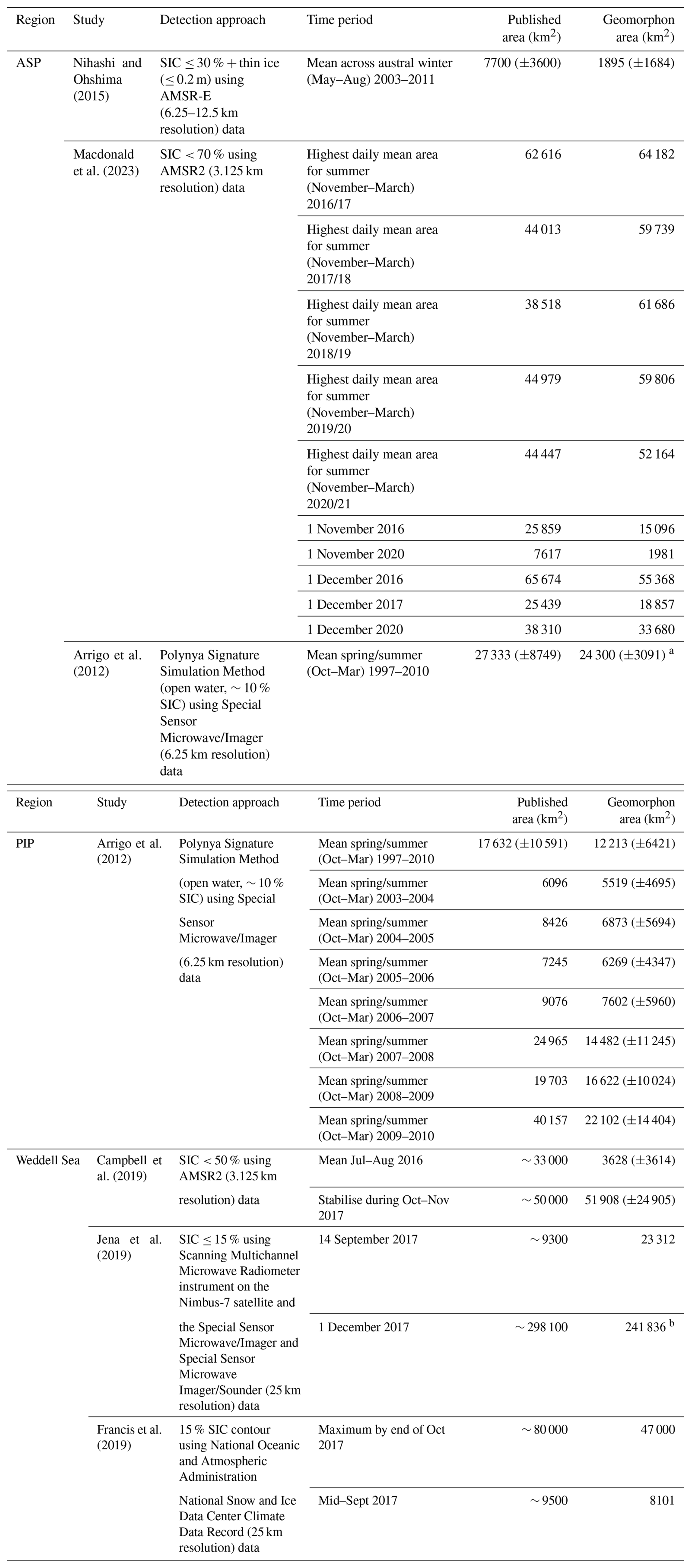
^a ASMR-E ASI sea ice concentration data spanning 2002–2010 used to calculate this value, ^b Estimated using a search distance parameter value of 100 map cells to represent the exceptionally large December 2017 Weddell Sea Polynya. All other Weddell Sea geomorphon estimates were produced using the optimised regional parameter set (search = 40 map cells).

4.3 Robustness to Geomorphon Parameter Selection and Sea Ice Concentration Uncertainty

While the geomorphon framework showed close agreement with threshold-based methods and published polynya extents, it is equally important to understand how sensitive these estimates are to the choice of geomorphon parameters and uncertainty in the underlying sea ice concentration data. Both sources of uncertainty have the potential to influence the delineation of polynya boundaries and, consequently, the estimated polynya area. Quantifying these uncertainties therefore provides an indication of the robustness of the geomorphon approach across different polynya states and identifies the conditions under which the method is most sensitive.

Uncertainty was not uniform across the seasonal cycle. Both parameter selection and sea ice concentration uncertainty were generally greatest during developing and decaying polynya conditions, whereas substantially smaller uncertainties were obtained for peak, frozen-over and absent scenarios (Table 3). This pattern is consistent with the changing morphology of polynyas throughout their seasonal evolution. During periods of opening and closure, polynya boundaries are often poorly defined and characterised by mixtures of open water, thin ice and consolidated pack ice (Morales Maqueda et al., 2004; Heorton et al., 2017), making the exact boundary more sensitive to both geomorphon parameterisation and uncertainty in the underlying sea ice concentration field. In contrast, mature polynyas and frozen conditions exhibit stronger morphological contrasts, resulting in more stable classifications. Across the developing, peak and decaying polynya scenarios, uncertainty associated with the sea ice concentration observations generally exceeded that arising from geomorphon parameter selection (Table 3). This indicates that, once an appropriate parameterisation has been selected, the geomorphon framework introduces relatively little additional uncertainty to the resulting polynya area estimates. Instead, the variability in estimated area is largely governed by the uncertainty inherent within the input sea ice concentration data. The relatively small contribution of geomorphon parameter uncertainty therefore provides confidence that the morphology-based approach is robust and that the resulting polynya estimates primarily reflect the characteristics of the underlying observations rather than sensitivity to algorithm parameter selection. The frozen-over and absent scenarios differed slightly, with parameter uncertainty becoming comparable to, or exceeding, the uncertainty associated with the sea ice concentration data. This is expected because these scenarios contain very small or no polynya areas, meaning that minor differences in the delineation of isolated features can produce relatively large proportional changes in estimated area. Importantly, however, the absolute uncertainties remained small (< 1100 km²), indicating that the geomorphon framework produces stable area estimates even under conditions where polynyas are weakly developed or absent. However, further evaluation using independent observations of small, highly dynamic winter polynyas would be valuable to fully assess the performance of the approach under these conditions, particularly before application across further regions.

These results suggest that the geomorphon framework is relatively insensitive to reasonable variation in parameter selection and that confidence in the resulting polynya area estimates is primarily limited by the uncertainty of the input observations rather than the morphology-based classification itself. Although these findings provide confidence in the robustness of the approach for the two study regions considered here, further evaluation across additional polynya systems, sea ice concentration products and satellite sensors would help determine the broader transferability of the parameterisation and establish the extent to which similar levels of robustness are maintained under different environmental conditions.

4.4 Transferability and Applicability to Long-Term Polynya Monitoring

The results presented here demonstrate that the geomorphon framework can be successfully applied to both coastal and open-ocean polynyas using passive microwave sea ice concentration data. Across two contrasting Antarctic regions, the method remained robust over a range of seasonal conditions and produced polynya extents that compared well with both conventional threshold-based approaches and previously published estimates. These findings suggest that morphology-based classification represents a promising complementary framework for automated polynya detection, while also highlighting that parameter selection should remain appropriate for the spatial scale of the target polynya.

An important next step will be to undertake a systematic comparison of the growing range of automated polynya detection techniques. Recent studies have demonstrated increasing methodological diversity in automated polynya detection from satellite observations (e.g., Lin et al., 2024; Duffy et al., 2024; Landrum et al., 2026; Heuzé and Wong, 2025). However, these methods have generally been evaluated independently using different regions, datasets and performance metrics, making direct comparison difficult. Applying multiple automated methods to commonly used datasets would provide a more objective assessment of their relative strengths, limitations and suitability for different polynya types and environmental conditions.

Beyond methodological evaluation, future work should investigate the performance of the geomorphon framework across additional Antarctic and Arctic polynya systems, alternative passive microwave products and higher-resolution satellite observations. Evaluating the approach across different sensors and environmental settings would establish the extent to which the parameterisation developed here is transferable beyond the study regions considered. The computational efficiency and automated nature of the geomorphon framework also make it well suited to analysing long satellite time series, providing opportunities to investigate long-term variability in polynya occurrence, duration and morphology. Such datasets could subsequently support studies examining links between polynyas and ocean circulation, primary productivity, ecosystem dynamics and climate variability. To support future applications of the geomorphon framework, a recommended implementation workflow is provided in Appendix G (Fig. G1). The schematic summarises the principal stages involved in applying the geomorphon approach to sea ice concentration data, from selecting an appropriate dataset and geomorphon parameterisation through to generating polynya masks and estimating polynya area. Although individual parameter values should be selected according to the study objectives and characteristics of the input dataset, we hope this framework provides a transparent starting point that can be tested, refined and adapted for different polynya types, regions and data products.

5 Conclusions

This study demonstrates the value of applying the geomorphon algorithm to passive microwave sea ice concentration data as a novel, automated approach for identifying polynyas. Traditionally, polynya detection has relied on fixed sea ice concentration or sea ice thickness thresholds (Nakata et al., 2015; Ohshima et al., 2016; Monroe et al., 2021), which may not consistently capture the full spatial extent of polynyas under different seasonal conditions or across different study regions (Massom et al., 1998; Mohrmann et al., 2021). By contrast, although originally developed for terrestrial applications, the geomorphon framework identifies polynyas from the spatial morphology of the sea ice concentration field, providing a complementary automated approach to conventional threshold-based methods. The successful detection of both coastal and open-ocean polynyas across contrasting seasonal conditions, together with close agreement with published polynya extents and threshold-based approaches, demonstrates the potential of morphology-based classification for automated polynya detection.

The uncertainty analyses further showed that the geomorphon framework is robust to reasonable variation in parameter selection, with uncertainty associated with the underlying sea ice concentration observations generally exceeding that introduced by the geomorphon algorithm itself. Although additional evaluation across a wider range of regions, sea ice concentration datasets and automated detection methods is required, these results provide confidence that morphology-based approaches represent a promising direction for objective and reproducible polynya detection. Continued development and evaluation of automated detection frameworks will be important for generating consistent long-term records of polynya variability. Such records have important implications for understanding links between polynyas and top predator ecology (Gilchrist and Robertson, 2000; Labrousse et al., 2018), primary productivity (Arrigo and van Dijken, 2003; Arrigo et al., 2008), and conservation planning (Boothroyd et al., 2024), particularly in the rapidly changing polar oceans.

Appendix A: Representative sea ice concentration fields for the five Amundsen Sea and Weddell Sea scenarios

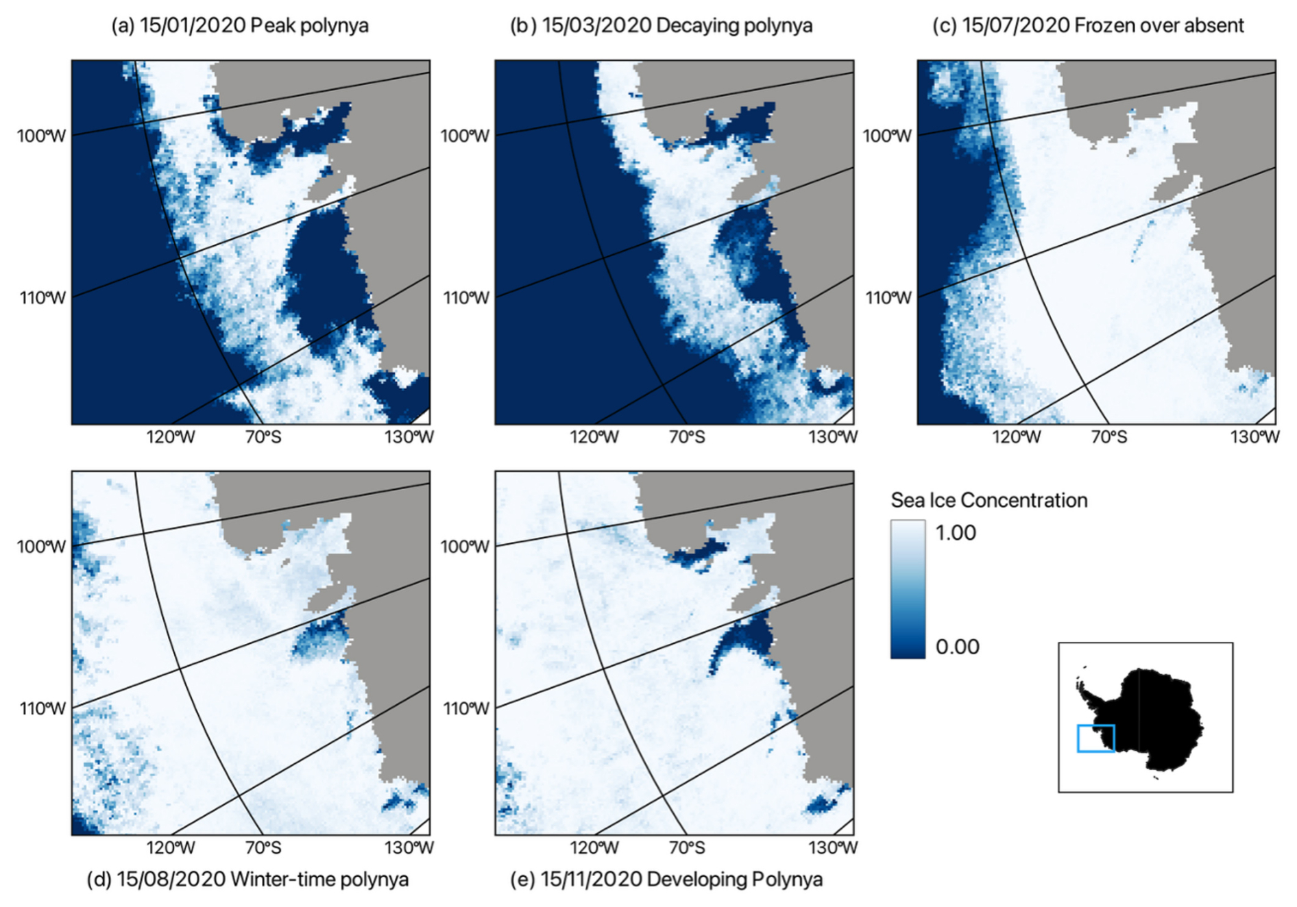
Figure A1 Representative sea ice concentration fields for the five Amundsen Sea 2020 scenarios. Daily data was obtained from the University of Bremen Archive, AMSR2 ASI sea ice concentration, version 5.4 (Melsheimer and Spreen, 2019).

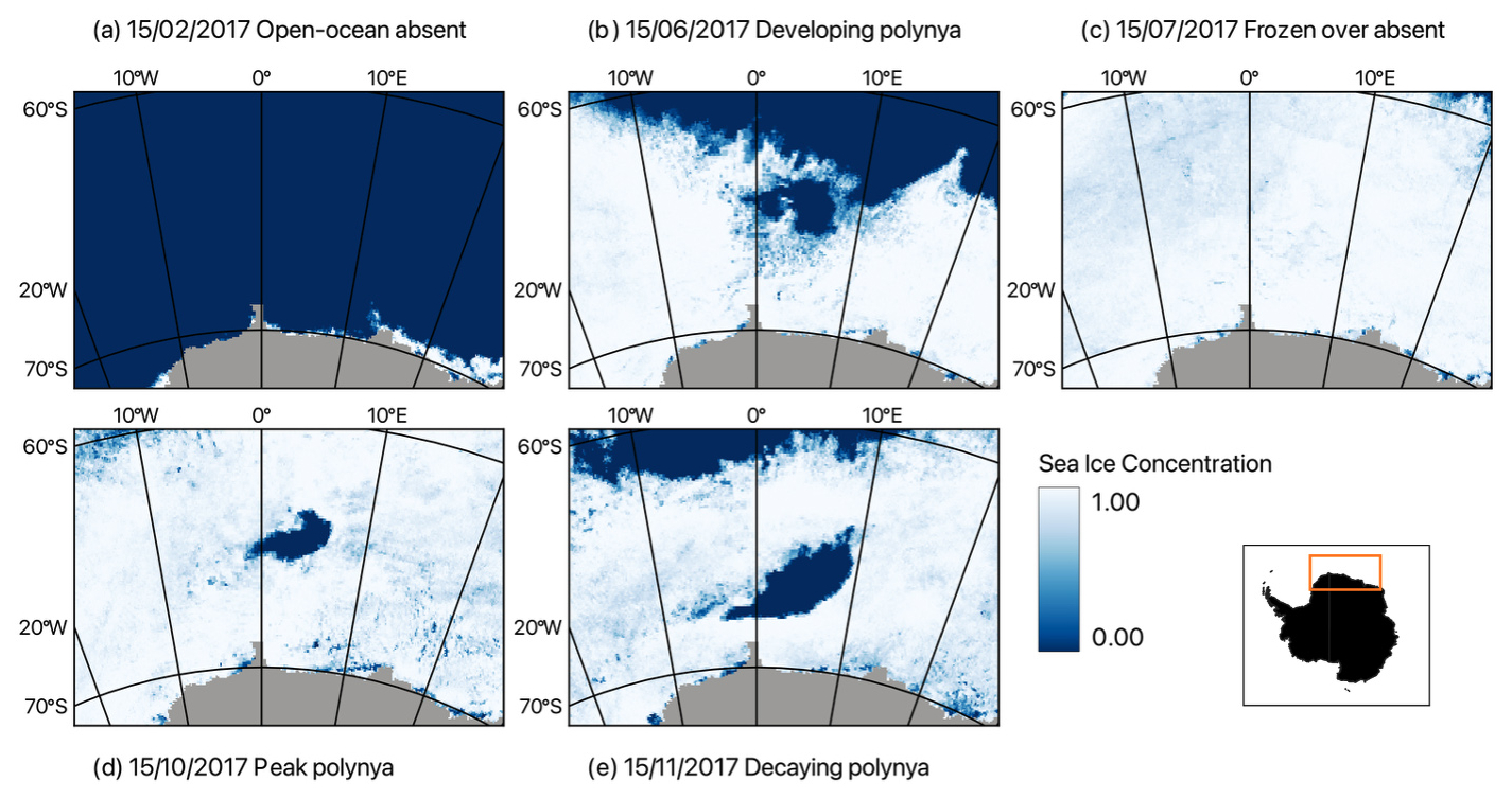
Figure A2 Representative sea ice concentration fields for the five Weddell Sea 2017 scenarios. Daily data was obtained from the University of Bremen Archive, AMSR2 ASI sea ice concentration, version 5.4 (Melsheimer and Spreen, 2019).

Appendix B: Geomorphon landforms assigned to areas classified as polynyas and non-polynyas by the threshold-based method

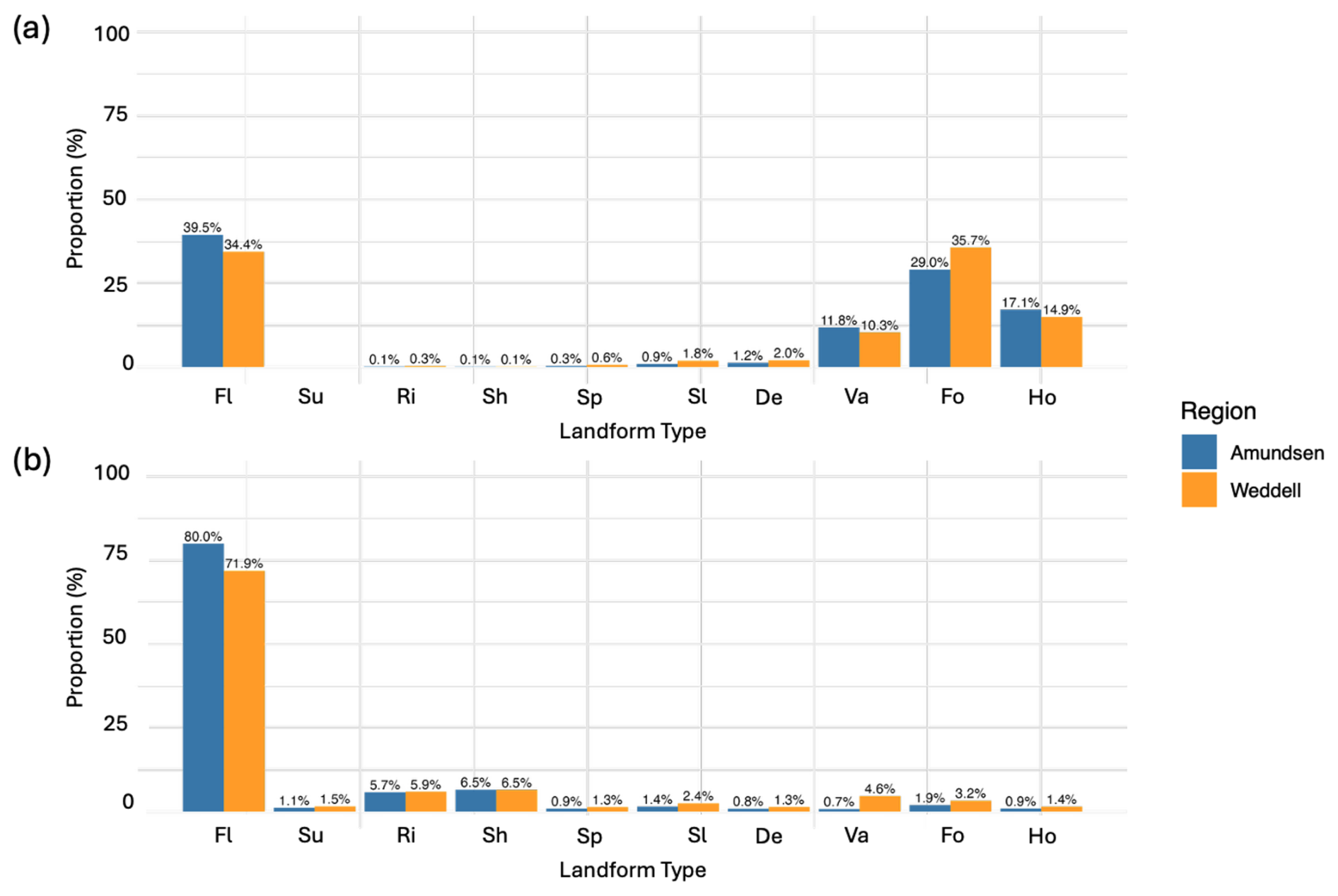
Figure B1 The proportion of geomorphon landforms (Fig. 2) assigned to (a) polynya and (b) non-polynya areas, defined by the ≤ 0.3 sea ice concentration threshold-based method, across all tested parameter combinations for both regions.

Appendix C: Precision and recall scores for geomorphon algorithm when compared to threshold-based method

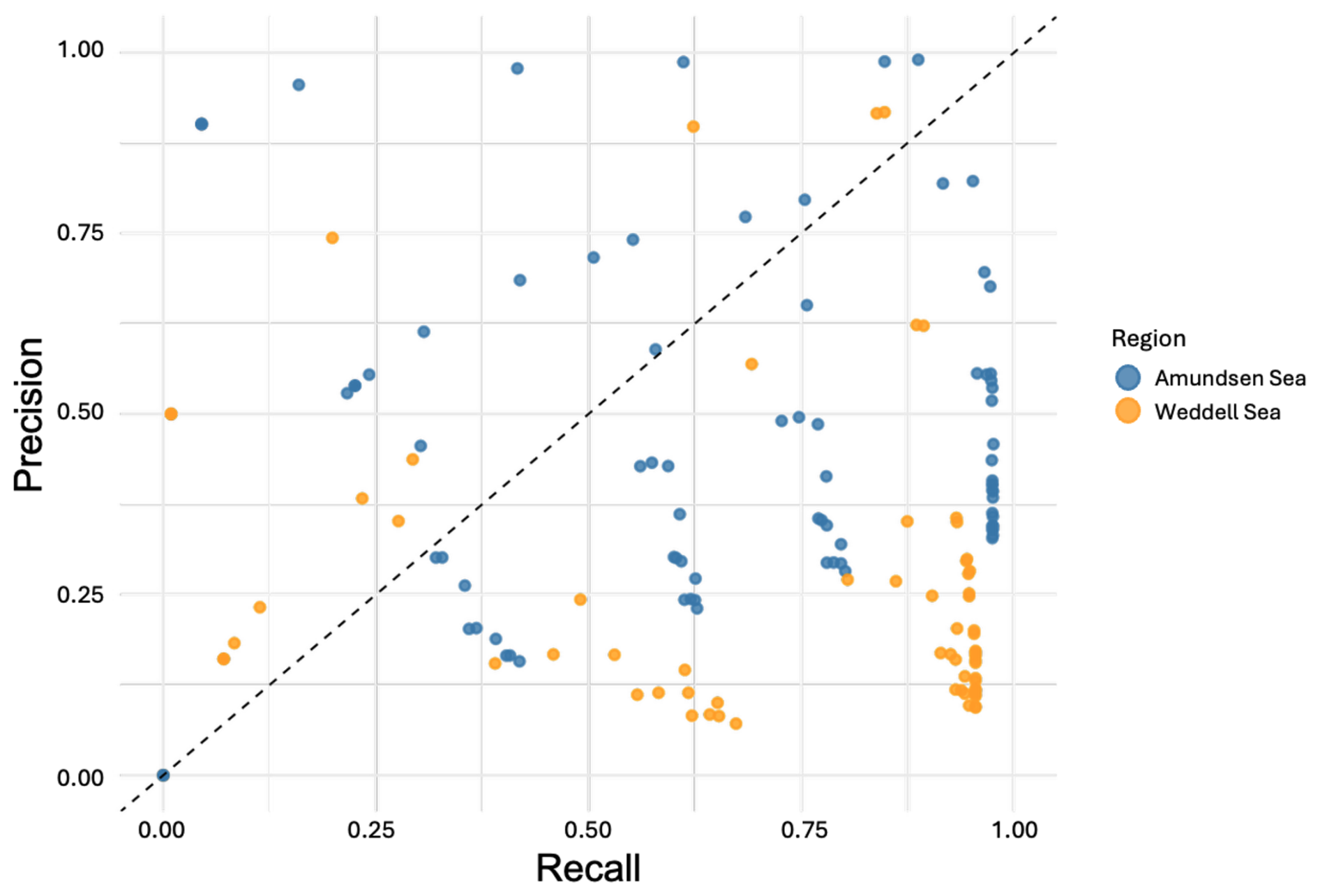
Figure C1 Precision-recall plot comparing the performance of the geomorphon algorithm across parameter combinations for the Amundsen (blue) and Weddell (orange) Seas. Each point represents a unique parameter configuration, evaluated by its precision and recall scores based on comparison to polynyas defined by the sea ice concentration method. The dashed diagonal line indicates equal precision and recall. Points closer to this line represent balanced performance, while deviations suggest a trade-off between the two metrics.

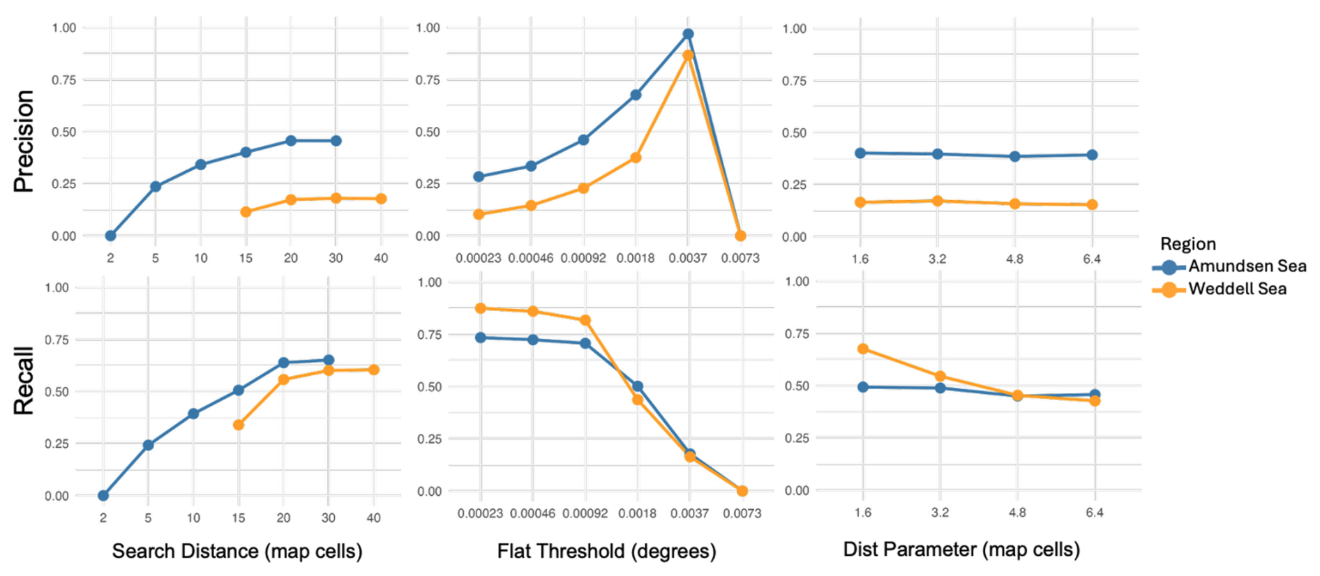
Figure C2 Precision (top row) and recall (bottom row) scores for different parameter values (search, flat, dist) used in iterations of the geomorphon algorithm in the Amundsen (blue) and Weddell (orange) Seas. Precision and recall scores are calculated as averages for each parameter value, considering its combination with all values from the other two parameters in each iteration.

Appendix D: Performance of geomorphon algorithm parameters across seasonal sea ice conditions

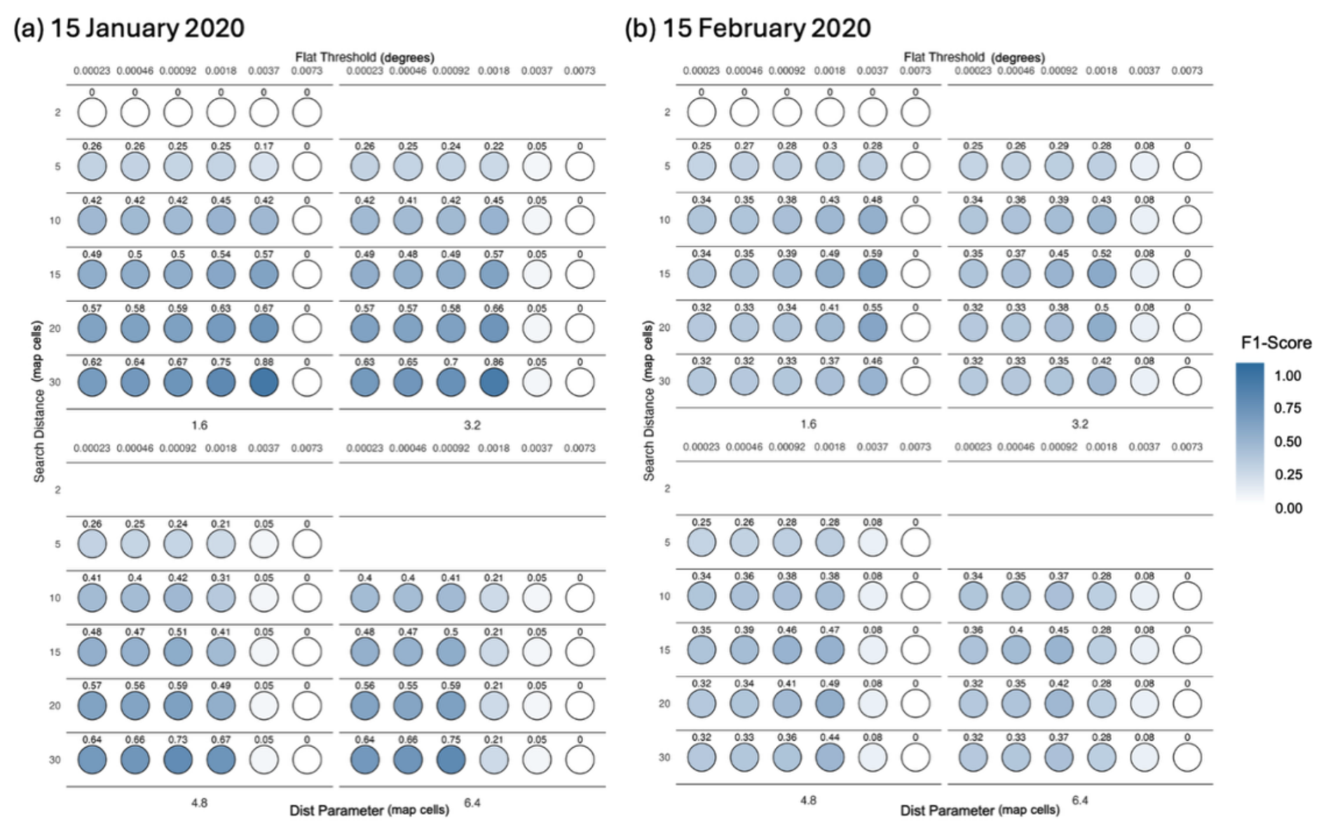
Figure D1 Seasonal performance of all valid geomorphon parameter combinations during austral summer (December–February) for the Amundsen Sea (2020), evaluated using daily sea ice concentration fields from the 15th day of each month. Bubble colour indicates the F1-score for months containing one or more reference polynya pixels and the False Positive Rate (FPR) for months in which no reference polynya pixels were present. Bubble size is proportional to the corresponding performance metric. Parameter combinations are arranged according to the search parameter (map cells), flat threshold (degrees), and dist parameter (map cells). The representative parameter tuning case study, 15 December 2020 for the Amundsen Sea, is presented separately in Fig. 5.

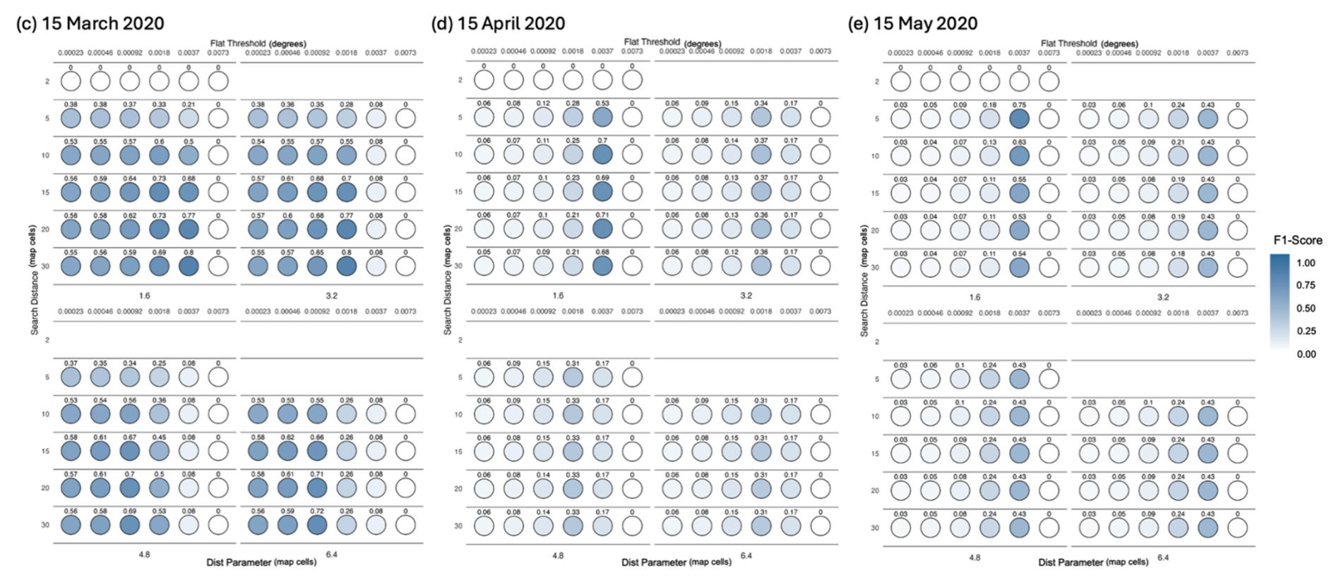
Figure D2 Seasonal performance of all valid geomorphon parameter combinations during austral autumn (March–May) for the Amundsen Sea (2020), evaluated using daily sea ice concentration fields from the 15th day of each month. Bubble colour indicates the F1-score for months containing one or more reference polynya pixels and the False Positive Rate (FPR) for months in which no reference polynya pixels were present. Bubble size is proportional to the corresponding performance metric. Parameter combinations are arranged according to the search parameter (map cells), flat threshold (degrees), and dist parameter (map cells). The representative parameter tuning case study, 15 December 2020 for the Amundsen Sea, is presented separately in Fig. 5.

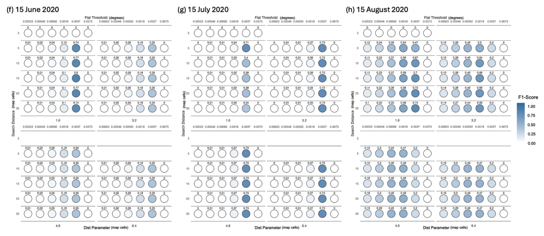
Figure D3 Seasonal performance of all valid geomorphon parameter combinations during austral winter (June–August) for the Amundsen Sea (2020), evaluated using daily sea ice concentration fields from the 15th day of each month. Bubble colour indicates the F1-score for months containing one or more reference polynya pixels and the False Positive Rate (FPR) for months in which no reference polynya pixels were present. Bubble size is proportional to the corresponding performance metric. Parameter combinations are arranged according to the search parameter (map cells), flat threshold (degrees), and dist parameter (map cells). The representative parameter tuning case study, 15 December 2020 for the Amundsen Sea, is presented separately in Fig. 5.

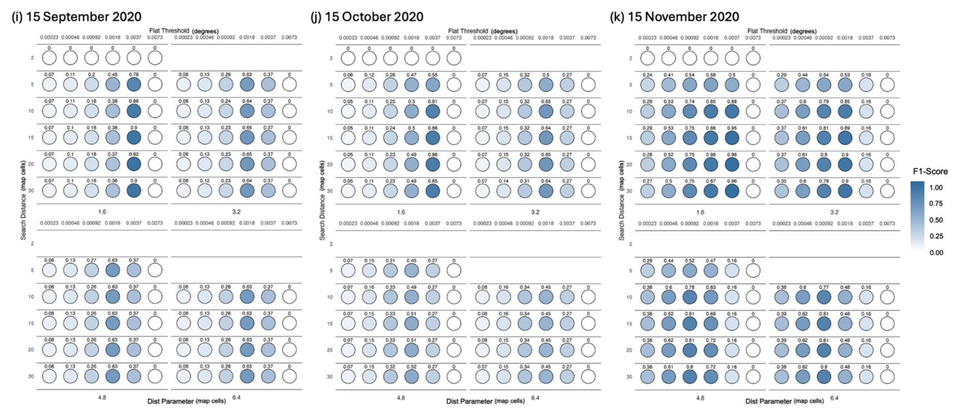
Figure D4 Seasonal performance of all valid geomorphon parameter combinations during austral spring (September–November) for the Amundsen Sea (2020), evaluated using daily sea ice concentration fields from the 15th day of each month. Bubble colour indicates the F1-score for months containing one or more reference polynya pixels and the False Positive Rate (FPR) for months in which no reference polynya pixels were present. Bubble size is proportional to the corresponding performance metric. Parameter combinations are arranged according to the search parameter (map cells), flat threshold (degrees), and dist parameter (map cells). The representative parameter tuning case study, 15 December 2020 for the Amundsen Sea, is presented separately in Fig. 5.

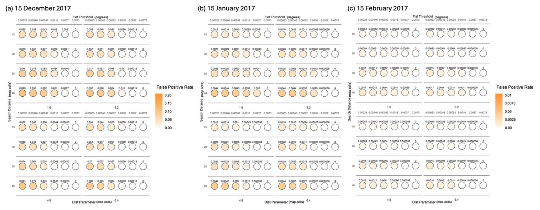
Figure D5 Seasonal performance of all valid geomorphon parameter combinations during austral summer (December–February) for the Weddell Sea (2017), evaluated using daily sea ice concentration fields from the 15th day of each month. Bubble colour indicates the F1-score for months containing one or more reference polynya pixels and the False Positive Rate (FPR) for months in which no reference polynya pixels were present. Bubble size is proportional to the corresponding performance metric. Parameter combinations are arranged according to the search parameter (map cells), flat threshold (degrees), and dist parameter (map cells). The representative parameter tuning case study, 15 October 2017 for the Weddell Sea, is presented separately in Fig. 4.

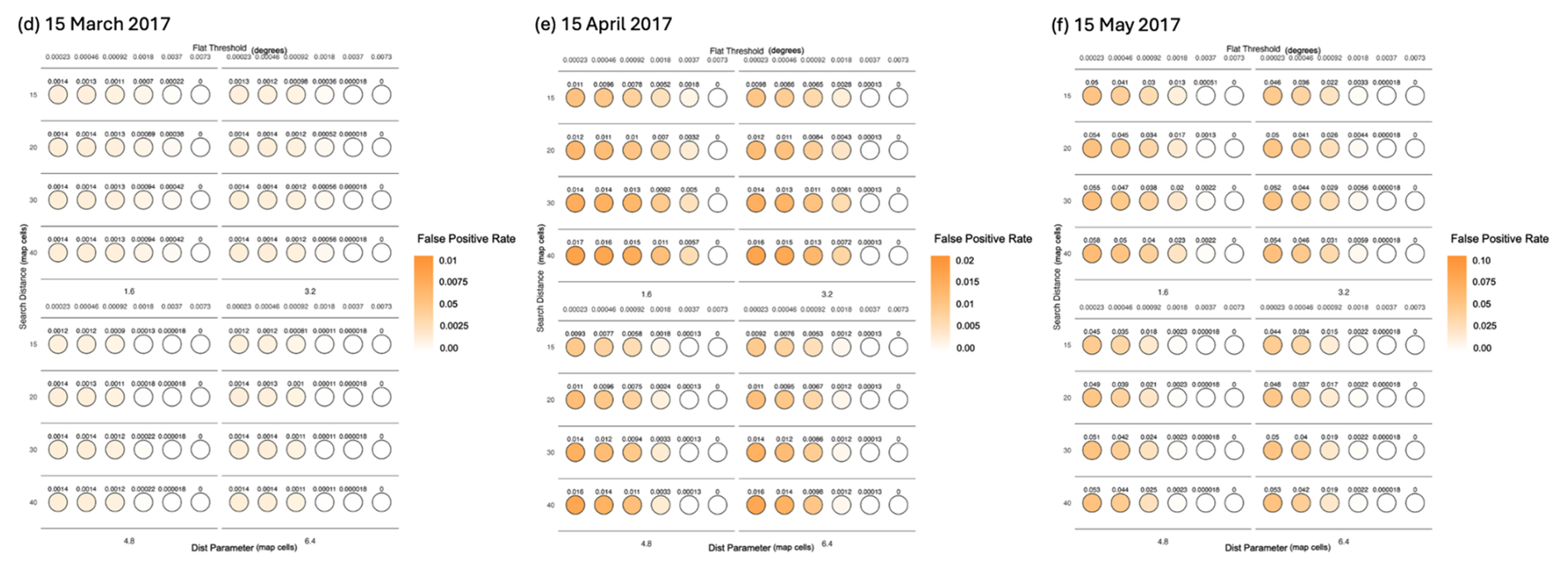
Figure D6 Seasonal performance of all valid geomorphon parameter combinations during austral autumn (March–May) for the Weddell Sea (2017), evaluated using daily sea ice concentration fields from the 15th day of each month. Bubble colour indicates the F1-score for months containing one or more reference polynya pixels and the False Positive Rate (FPR) for months in which no reference polynya pixels were present. Bubble size is proportional to the corresponding performance metric. Parameter combinations are arranged according to the search parameter (map cells), flat threshold (degrees), and dist parameter (map cells). The representative parameter tuning case study, 15 October 2017 for the Weddell Sea, is presented separately in Fig. 4.

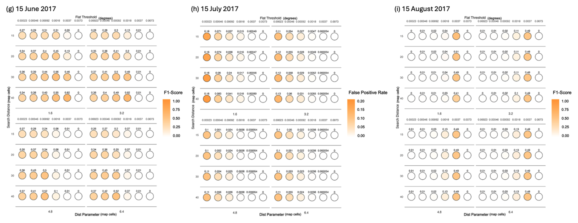
Figure D7 Seasonal performance of all valid geomorphon parameter combinations during austral winter (June–August) for the Weddell Sea (2017), evaluated using daily sea ice concentration fields from the 15th day of each month. Bubble colour indicates the F1-score for months containing one or more reference polynya pixels and the False Positive Rate (FPR) for months in which no reference polynya pixels were present. Bubble size is proportional to the corresponding performance metric. Parameter combinations are arranged according to the search parameter (map cells), flat threshold (degrees), and dist parameter (map cells). The representative parameter tuning case study, 15 October 2017 for the Weddell Sea, is presented separately in Fig. 4.

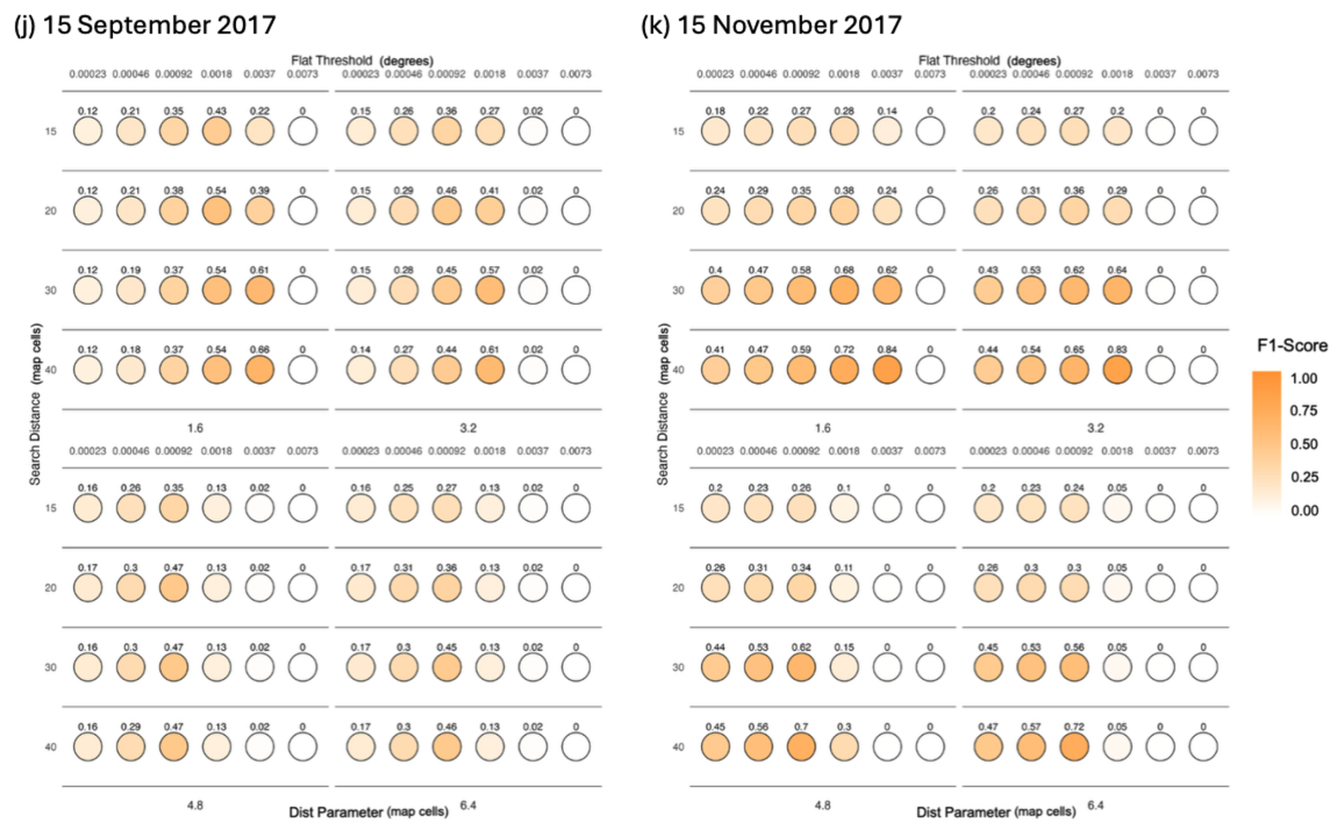
Figure D8 Seasonal performance of all valid geomorphon parameter combinations during austral spring (September–November) for the Weddell Sea (2017), evaluated using daily sea ice concentration fields from the 15th day of each month. Bubble colour indicates the F1-score for months containing one or more reference polynya pixels and the False Positive Rate (FPR) for months in which no reference polynya pixels were present. Bubble size is proportional to the corresponding performance metric. Parameter combinations are arranged according to the search parameter (map cells), flat threshold (degrees), and dist parameter (map cells). The representative parameter tuning case study, 15 October 2017 for the Weddell Sea, is presented separately in Fig. 4.

Appendix E: Parameter combination retention across representative polynya scenarios for the Amundsen Sea 2020 and the Weddell Sea 2017 using F1-scores and FPR

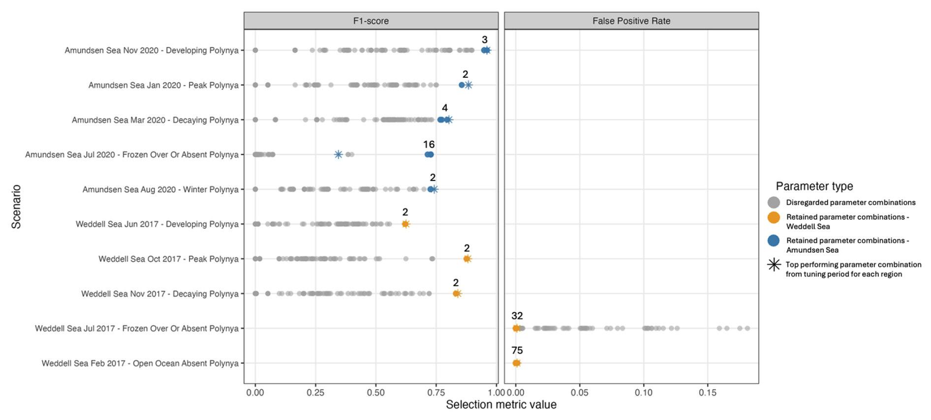
Figure E1 F1-score (left) and false positive rate (right) for all tested geomorphon parameter combinations across the ten seasonal polynya scenarios (Figs. A1 and A2). Grey points show discarded parameter combinations, while coloured points indicate retained parameter combinations (orange = Weddell Sea, blue = Amundsen Sea). Asterisks denote the top performing parameter combination from the tuning periods for each month (Fig. 6), and numbers indicate the total number of retained parameter combinations for each scenario.

Appendix F: Comparison of polynya determination by sea ice concentration threshold-based method and geomorphon algorithm for the ASP in the Amundsen Sea 15 February 2020

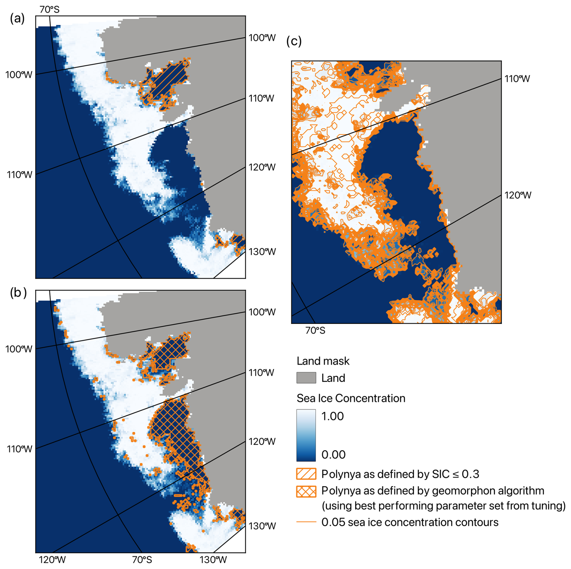
Figure F1 Comparison of polynya detection for the Amundsen Sea Polynya (ASP) on 15 February 2020 using (a) the ≤ 0.3 sea ice concentration threshold method and (b) the geomorphon algorithm (best-performing parameter combination). (c) Enlarged view of the central ASP with orange contours represent 0.05 sea ice concentration intervals. In this example, the threshold-based method identifies a connection between the polynya and the adjacent open ocean, whereas the geomorphon algorithm continues to delineate the feature as a distinct enclosed polynya.

Appendix G: Schematic showing recommended workflow for future applications of the geomorphon method for polynya detection

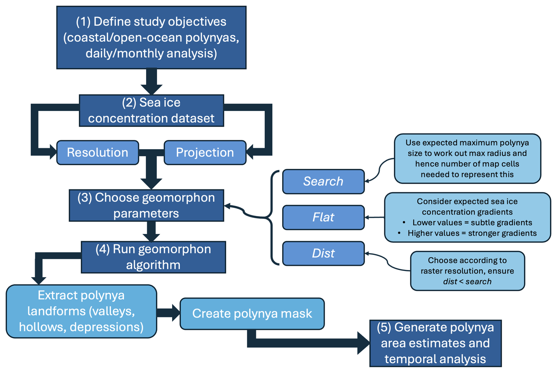
Figure G1 Recommended workflow for applying the geomorphon framework to passive microwave sea ice concentration data for automated polynya detection. The schematic outlines the principal stages of the workflow, including study design, dataset selection, geomorphon parameter selection, landform extraction and generation of polynya area estimates.