High current speed events in a harbor channel driven by resonant sub-hourly sea level dynamics: an example from Varna, Black Sea

Current and sea-level observations in the 2.4 km-long, 300 m-wide channel between Varna Lake and the Black Sea, conducted by three novel Hydromast stations with a 1 min resolution, revealed that moderate sub-hourly dynamics were occasionally interrupted by high-amplitude oscillations with a period of a few tens of minutes. The resonant excitation of the events was studied using barotropic 1D analytical and numerical methods. Basic features of high-intensity sub-hourly variations can be interpreted as linear barotropic long waves in a sea-channel-lake system with resonant and damped forcing. The observed 37 min oscillations, identified from the power spectra, spectrogram, and wavelet analysis, can be explained as the first mode of the channel-lake system. Another period of 19 min resembles the zero, quarter-wave mode of the channel and the second mode of the channel-lake system. During the measurement period, two high-amplitude events were highlighted. One of the events is interpreted as having been caused by a meteotsunami; moderate meteorological conditions prevailed; strong channel oscillations began abruptly and lasted for a few cycles. The second event occurred more than 5 h after landward winds up to 20 m s⁻¹. The observed maximum changes in current and sea level – up to 0.8 m s⁻¹ and 0.8 m, respectively, over 10 min – are harmful to ship navigation, harbor operations, and coastal management. Building on these observations, approaches for detecting and forecasting strong sub-hourly oscillations are discussed.

1 Introduction

Coastal embayments and channels respond to forcing from the open sea, under the control of weather variability, in a multitude of physical mechanisms. It was discovered a long time ago that coastal dynamics, encompassing waves, currents, and turbulence, may include tidal effects, barotropic and baroclinic self-oscillations (seiche) excited in topographically bounded domains, and different transformations of wind waves. An important component of variability arises from waves, which can be divided into short, non-hydrostatic waves with periods typically less than a minute, and long waves that are vertically in a hydrostatic balance and may be influenced by the Earth's rotation (LeBlond and Mysak, 1981).

Oscillations in semi-enclosed basins and channels (Miles, 1974; Rabinovich, 2009) include Helmholtz-type oscillations of a basin connected to the sea by a narrow channel (Miles and Munk, 1961; Méhauté et al., 1962), and seiche in elongated semi-enclosed basins (Giese and Chapman, 1993; see also the textbook by Cushman-Roisin and Beckers, 2011). The seiches often have half-wave (Cummins et al., 2010) or quarter-wave (Cerralbo et al., 2014; Zheng et al., 2024) character. Both wave types may exhibit resonant responses to external forcing (Miles and Lee, 1975) and include nonlinear effects (Maas, 1997; Doelman et al., 2002). The resonant modes are often associated with the diurnal or semidiurnal tides (Maas, 1997; Luettich et al., 2002). Sub-hourly oscillations with a period of a few tens of minutes may be excited during atmospheric low-pressure events when stronger high-frequency atmospheric pressure disturbances occur (Sammartino et al., 2014). At sub-hourly periods, moving atmospheric pressure systems can generate coastal edge waves on the ocean side of channels and river mouths (Sun and Niu, 2021) and form meteotsunamis through Proudman resonance, when the transient speed of weather patterns equals the phase speed of long gravity waves (Williams et al., 2021; Vilibić et al., 2025).

Ocean state observations and forecasts are usually exchanged at 1 h intervals, which is sufficient for detecting the main features of tides and storm surges. However, the need for sub-hourly resolution in routine meteorological and oceanographic data was recognized as early as the 1950s (Van der Hoven, 1957), who showed spectral peaks in wind data at about 1 min. In coastal oceanography, water levels are recorded at 1 min intervals in many locations since the 1980s (Miller and Luscher, 2019). Presently, there are initiatives to manage high-resolution water level data, such as SHELDA (Sub-hourly European Quality Controlled Sea Level Dataset; Balić and Šepić, 2025), but standard data exchange for now and forecasts, such as in Copernicus Marine Service, uses a 1 h resolution.

Sub-hourly water dynamics contribute to the (1) extremely high water levels during the storm surges (Medvedev et al., 2022; Ruić et al., 2023), (2) anatomy of seismic tsunamis (Catalán et al., 2025), (3) events of high currents at topographic constrictions (even when water level disturbances are small), disturbing navigation and/or impacting the sediments and coastline (Seo et al., 2024; Kanarik et al., 2025).

Detection and analysis of sub-hourly dynamics are enabled by recent developments in observation techniques that make high-frequency current observations available at moderate costs. Among the applications of these new methods, we note the first presentation of the Varna Port Case Study (Egerer et al., 2025), which used Hydromast observations to study the hydrodynamic patterns in the area.

The purpose of this work is to gain a better understanding of flow dynamics in channels to aid pilots in navigating ships, with a long-term goal of predicting strong flows and promptly informing pilots of changing currents. The study was designed to advance knowledge of water movement patterns, which could support port management and navigation safety and contribute to environmental impact assessments. The study aims to explore events with high current speeds associated with resonant sub-hourly sea-level dynamics in the harbor system comprising a sea bay and narrow channels connecting to the upstream lake and river. The study uses the same data from the Varna Harbor area as analyzed by Egerer et al. (2025).

The paper is organized as follows. After the introduction, Sect. 2 presents the data and methods, beginning with a description of the study area. The presentation of observations includes dedicated current and sea-level observations using the Hydromast system, as well as background sea-level and meteorological observations conducted by the Bulgarian research authorities. Data used from the EU Copernicus Marine Service are also outlined. Further sections present the data analysis. Section 3 on results presents the observed water-level and current time series, together with meteorological data, and analyzes sub-hourly variability. A detailed analysis of high-current-speed events follows oscillatory analysis. The observed variability is subject to interpretation using the 1D shallow-water equations outlined in the Appendix. In Sect. 4, the results are discussed with respect to the mechanisms driving high-current-speed events and the prospects for predicting them in the interests of port authorities and ship captains. Conclusions are presented in Sect. 5.

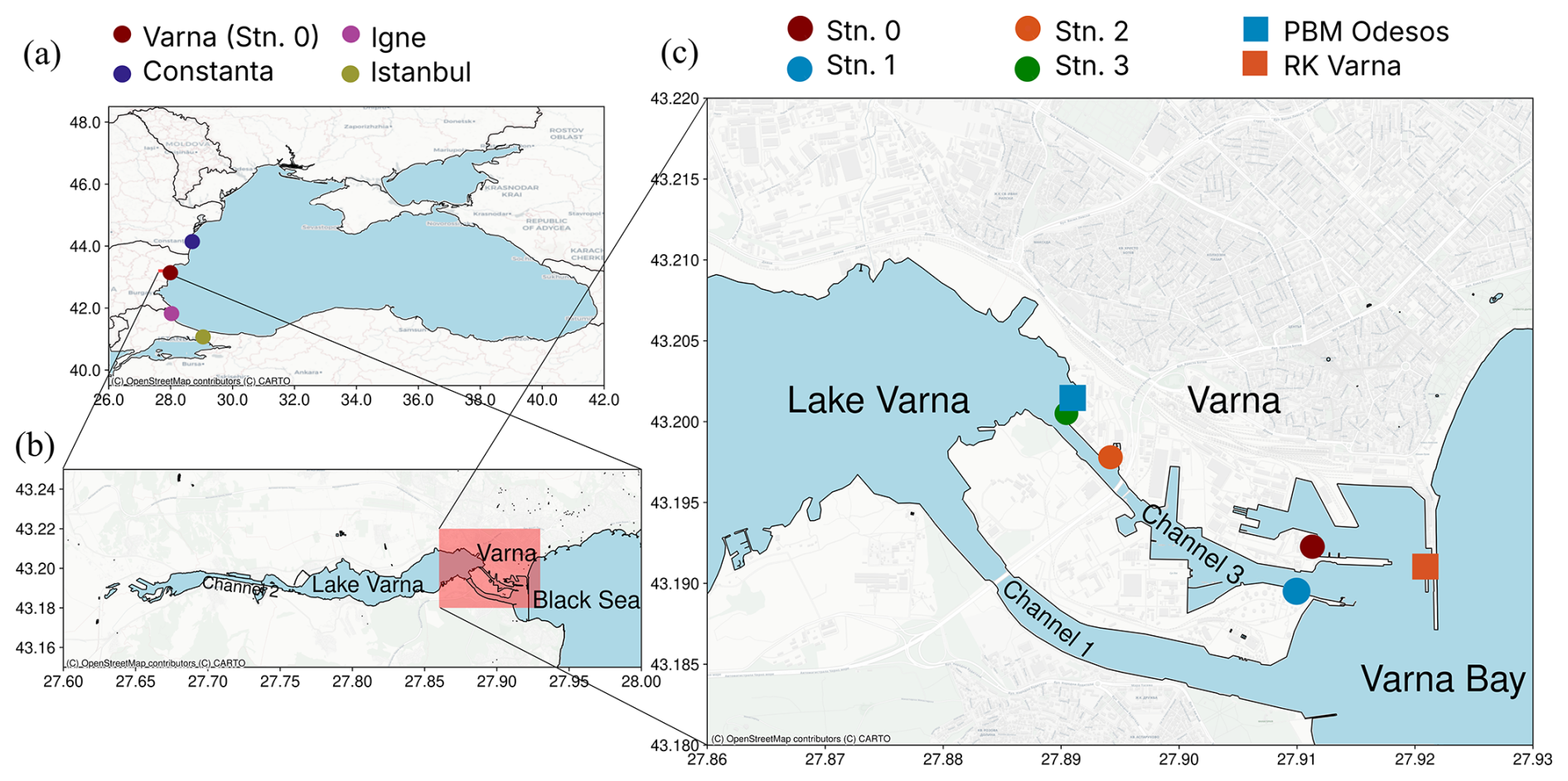
Figure 1 (a) Location of the study area, shown on the map of the Black Sea. The western coastal stations where data are shared within the Copernicus Marine Service data © European Union, 2026 are indicated on the map. (b) Map of the Varna region. (c) Map of the study area displaying the locations of the observation sites. Details of observation points are given in Table 1.

2 Data and Methods

2.1 Study area

The focus of the study is the marine area of the city of Varna, Bulgaria, located in the western part of the Black Sea (Fig. 1). Port of Varna, extending from the seaside through the navigational channels to Lake Varna and the upstream Lake Beloslav, is the largest seaport complex in Bulgaria and an important transport hub of the Black Sea. It handles more than 8.4 million  t of cargo annually, specializing in container freight. The East and West Terminals, together with specialized harbors, have a total of 71 berths, with a length that exceeds 100 m (ORDER No Z-160/VARNA, 2026); they can handle ships up to 50 000 GT (gross tons). It is anticipated that larger vessels, about 200 m in length and 10 m in draft, may cause significant hydrodynamic disturbances in the navigation channels.

The Black Sea is a deep (maximum depth about 2200 m) semi-enclosed sea in which freshwater input, together with restricted water exchange with the Mediterranean, forms an estuarine basin. The water masses have distinct vertical stratification; together with river input in coastal areas, density gradients and wind stress create cyclonic circulation of the sea, consisting of coastal rim current and unsteady circulation cells within the deep basins. Tides are rather weak in the Black Sea, with diurnal and semidiurnal periods having amplitudes typically less than 0.2 m in the sea level time series. There are spectral signatures of large-scale self-oscillations (seiche) at periods 10.7, 5.8, 4.9, and 4.1 h (Medvedev, 2022).

On the seaside, the region of interest includes Varna Bay, the second-largest Bulgarian bay, with an approximate width of 3 km and a length of 5 km, defined by coastal capes. The currents and sea level of the western coastal region of the Black Sea are impacted by the hydrodynamics of the whole sea area (Stanev, 2005). West of Varna Bay lies Varna Lake, an 11 km-long, 2 km-wide lake that receives freshwater from upstream Beloslav Lake and the rivers (Fig. 1b). The lake is connected to the sea by two navigation channels (Fig. 1c). The Varna Lake-Varna Bay system facilitates freshwater inflow into Black Sea and saline seawater flow into Varna Lake (Yakushev et al., 2026). The depths of the region are shallow, up to 20 m in the Varna Bay and Varna Lake, and less in the navigation channels.

The study site is in a humid subtropical climate zone. The mean wind is oriented alongshore in the coastal sea area to the south (Stanev and Ricker, 2019). Regarding wind variability (mainly due to the passage of synoptic weather systems), the wind rose (Panaitescu et al., 2023) shows mainly alongshore winds in either southerly or northerly directions. The winds are modified in the land-bound Varna Bay-Varna Lake system, located in a valley between the northern and southern hills. Orographic steering, combined with sea breezes, guides the winds cross-shore along the valley (Barantiev et al., 2011; Trukhchev et al., 2025). Storms are usually observed during winter, when cold air masses come from the north. Sea breezes occur during the warmer seasons; they may create strong diurnal signals in cross-shore winds and air temperature.

The area of interest has been largely influenced by intensive human activity for coastal protection and urban socio-economic development. The northern channel (Channel 3, also known as the Old Canal) is older (commenced in 1906) and narrower. It serves multiple terminals in Port Varna – East, including Multipurpose terminal Odesos PBM – Varna, and plays a crucial role in managing large-ship traffic. The southern channel (Channel 1) is newer (1976) and wider and is the main waterway connection between the Black Sea's Varna Bay and Lake Varna. The Channel 2 connects Lake Varna to Lake Beloslav and forms the primary connection between the Black Sea and the Port of Varna – West connection. The channels 1 and 3 have a bending shape: they are rotated clockwise by about 20° from the west-east direction along the seaside and by about 40° near the lake. The Varna Lake-Varna Bay system facilitates freshwater inflow into Black Sea and saline seawater flow into Varna Lake (Yakushev et al., 2026). Typical salinity at the lakeside is 12 g kg⁻¹, and on the adjacent Black Sea side is 17 g kg⁻¹. The average river discharge to the lake area is 3 m³ s⁻¹. Using the Knudsen salt and water budget for stationary flows, this freshwater input is balanced by a seawater inflow of 7.2 m³ s⁻¹and a lake water outflow of 10.2 m³ s⁻¹.Therefore, long-term freshwater-induced currents are well below 0.01 m s⁻¹, and they should not interfere with current oscillations. A salinity difference of 5 g kg⁻¹ creates a density difference of about 4 kg m⁻³, which, at a depth of 10 m, is balanced by a sea level difference of 0.04 m. This sea-level threshold is easily exceeded by diurnal and semidiurnal oscillations and storm surges, indicating a dominant barotropic flow regime in the channels.

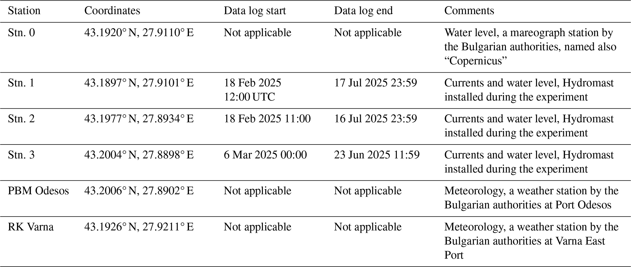
Table 1 List of observation points and data availability for the experimental period starting from 18 February 2025.

2.2 Observations

The study was conducted in Channel 3. The experimental setup involved installing flow measurement devices, called Hydromasts (Egerer et al., 2024), at three locations in the port area, with the measurement sites shown in Fig. 1 and exact data presented in Table 1.

The Hydromast is a flow-monitoring device that uses a 3D Hall-effect sensor to measure direction and velocity at a fixed point. The Hydromast operates via a positively buoyant mast connected to a flexible membrane, allowing it to respond freely to the surrounding flow. The instantaneous mast deflection is measured using a 3D Hall-effect sensor, from which current velocity and direction are determined. In addition, it is equipped with absolute pressure and temperature sensors. These devices have been shown to provide accurate measurements across various marine applications (Egerer et al., 2025; Eelsalu et al., 2025).

Measurement locations were chosen to avoid interfering with port activities and to minimize the risk of damage. Station 1 (labeled Stn. 1) was positioned near the sea boundary of the Port of Varna channel, under a floating dock, allowing flow measurements with minimal obstructions. Station 2 (Stn. 2) was in the middle of the narrow port channel connecting the Black Sea's Varna Bay to Varna Lake, and Station 3 (Stn. 3) was next to the lake boundary of the channel. At Stn. 1, the installation is in a free-flow area, whereas at Stn. 2 and Stn. 3, the sensors are installed next to a concrete pier protruding about 40 cm from the pier. All sensors were placed 0.5 m above the bottom at depths of approximately 3.5 m.

Water level data were also obtained from the near-real-time (NRT) in situ quality-controlled Copernicus Marine service. In the study area, the “Varna station” of the Black Sea in situ network provided standard hourly observations; upon request, 1 min-resolution data were also obtained at a location labeled Stn. 0. Meteorological data (wind speed and direction, atmospheric temperature, and pressure) were obtained with a resolution of 10 min from the Port Varna meteorological stations, RK Varna and PBM Odesos, as shown in Fig. 1.

The experimental period started on 18 February 2025, when stations 1 and 2 came online, followed by Stn. 3 on 6 March 2025 (Table 1). Among the datasets with different lengths and gaps, the three-month period from 18 February to 18 May 2025 was selected for the data analysis.

The Hydromast records all data at 50 Hz. The collected raw data is processed following Egerer et al. (2024) to get velocity and direction estimates. The Hydromast devices with a mast length of 500 mm were used at all three sites, providing reliable velocity estimates ranging from 0.06 to 0.6 m s⁻¹. For this work, the data is downsampled to 0.0166 Hz (1 min).

The pressure logger records absolute pressure. The absolute pressure readings are corrected for atmospheric pressure using the RK Varna and PBS Odesos weather stations at the Varna port. In addition, correction with respect to the temperature is done using the following equation:

$$\begin{array}{}\text{(1)}& P_{\text{hm}}=[P_{\text{hm}\mathrm{0}}-(a{T}_{\text{hm}}+b\left)\right]-P_{\text{ref}},\end{array}$$

where T_hm is the temperature reading for the Hydromast in the water, a and b are empirically determined constants, and P_ref is a pressure sensor bias value ensuring that in air at the same temperature, P_hm and atmospheric pressure P_atm are equal.

2.3 Analysis methods

The 1 min average velocity, water column height, and direction were calculated by grouping the data into 1 min bins and computing the arithmetic means for each bin. The false data recordings, identified by data quality assurance filters, were removed and replaced with NaN (Not a Number) values for further analysis. Shorter-scale processes lasting less than 1 min were not considered relevant to this study.

To find the dominant oscillation frequency in the channel, the power spectral density (PSD) was calculated using the Welch method. The main analysis was performed using a window length of 10 d (14 400 min) and a window overlap of 5 d (7200 min) for all 4 stations (3 Hydromast and 1 Copernicus). The large window length was chosen to ensure the diurnal and semidiurnal cycles are included. However, given the extended duration and broad range of periodicities of interest, we tested multiple segment lengths and overlap parameters to evaluate the sensitivity of spectral features to analysis settings. For each configuration, the time series was partitioned into overlapping windows, and each window was tapered with an appropriate window function. Only those frequency peaks that consistently appeared across varying window sizes and overlap choices were retained for further analysis. This procedure ensures that detected spectral features are not artifacts of specific parameter settings. Furthermore, we required that consistent peaks be present across all measurement sites before inclusion in the final interpretation.

In addition, a comparison between pairs of stations in the frequency domain was performed using coherence analysis. The comparison included coherence calculations between all stations using 5 d segments and a 2 d overlap. Coherence quantifies the strength of the linear relationship between two time series as a function of frequency. Its values range from 0 to 1, where values close to 1 indicate a similar variability at a given frequency, while values close to 0 indicate little or no linear relationship. Hence, high coherence suggests that the stations respond to the same physical forcing at a given timescale.

Sub-hourly variations were analyzed using a monthly spectrogram over a period that covered the intense sub-hourly events. Furthermore, wavelet analysis was performed on the high-current-speed events. Wavelet transforms decompose a signal into components representing different frequency bands while preserving temporal localization, making them suitable for analyzing non-stationary signals whose frequency content varies over time. As the data span long periods and our interest includes high-frequency components during shorter events, we applied the discrete wavelet transform using the Daubechies wavelet (db4). This analysis examined how dominant frequency components evolve and identified frequency bands present at multiple measurement stations along the channel. To quantify the similarity of two selected water level signals at different frequency bands, the cosine correlation of wavelet coefficients was calculated across corresponding decomposition levels.

3 Results

3.1 Observed meteorological, water level, and current time series

The analyzed period of observations spanned three months, from the end of winter (18 February 2025) to the end of spring (18 May 2025), during which the mean air pressure was 1016 hPa (min 997, max 1038 hPa), equal to the long-term spring average. Mean wind speed was 4 m s⁻¹ as usual for the region; its instantaneous maximum amounted to 20 m s⁻¹. The mean wind vector was 0.62 m s⁻¹ directed to the west-southwest.

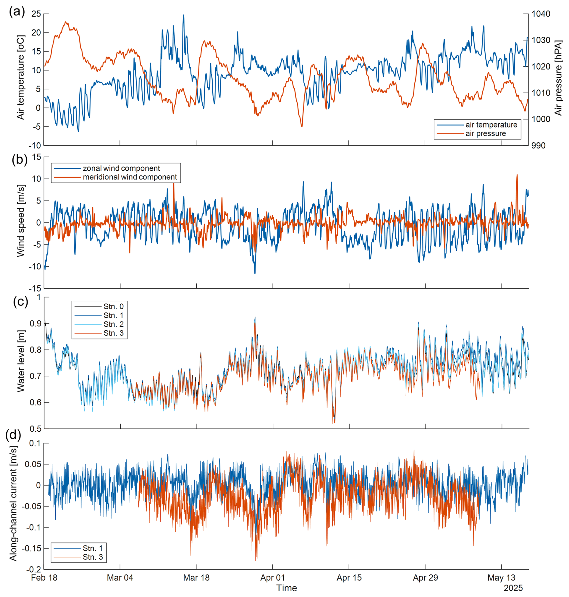
Figure 2 Time series of meteorological and oceanographic data with 1 h resolution. (a) Air temperature and air pressure, (b) zonal and meridional components of wind speed, (c) water level and (d) along-channel current speed (positive from lake to sea). Data from RK Varna (a, b), stations from Stn. 0 to Stn. 3 (c), and Stn. 1 and Stn. 3 (d).

In this sub-section, we consider variability based on hourly time series, filtered from the original, higher-resolution data using the Tuckey filter with a 2 h length (Fig. 2). Hourly resolution is also widespread in the dissemination of metocean observation and forecast data. We note that the variance of hourly changes in wind and water level exceeded 80 % of the total variance, including the high-resolution sub-hourly data. In the time series of currents, hourly changes covered only 30 % of the total variance.

Air temperature (Fig. 2a) generally reflected seasonal warming, ranging from −5 to +20 °C. Still, the weekly course depended on weather patterns over the area. High-temperature events above +20 °C were observed as early as the middle of March, during relatively low air pressure (Fig. 2a) and the strongest southerly winds (Fig. 2b).

Strong diurnal variations in temperature and the zonal (cross-shore) wind component developed during periods of stable air pressure, with temperature amplitudes up to 10 °C and zonal wind component amplitudes up to 10 m s⁻¹. Over the whole study period, deviations from daily mean zonal temperature and air temperature remained uncorrelated. During the seasonal warming period, from 20 April to 18 May, their correlation was 0.62. Nightly lower temperatures at the Varna meteorological station were associated with a land breeze (an offshore wind). Daytime faster heating over land, compared to that over the sea, corresponded to sea breeze (onshore wind). Therefore, differences in diurnal heat cycles over land and sea result in a drop in air temperature and associated winds (Abbs and Physick, 1992). Such breeze events were studied on the Bulgarian coast by Barantiev et al. (2011). The breeze caused an imprint on the water-level variations as well. Starting 27 April, usual semidiurnal oscillations at all four observation sites were suppressed, and diurnal oscillations became dominant (Fig. 2c), with daily extreme water levels observed during minimal zonal wind.

Water level variations occurred on top of the average sea level. Mean sea levels at Stn. 1 and Stn. 3 were 0.727 and 0.700 m, respectively, with the difference being within datum uncertainty. Water level variability during the study period, including the semidiurnal and diurnal oscillations noted above, was characterized by a standard deviation. It was 0.064 m in the seaside location and decreased to 0.058 m near the lake. The hourly water-level changes at all four stations were highly correlated, with Pearson correlation coefficient r > 0.96.

The highest hourly water level (0.92 m; Fig. 2c) was observed on 28 March. This high-water-level event is explained by the strongest winds, up to 20 m s⁻¹, blowing onshore from the east and northeast. Another local water-level maximum of 0.80 m was observed on 18 March; it has no obvious link to local wind forcing. The lowest water level of 0.52 m was observed on 12 April, when easterly onshore winds of about 6 m s⁻¹ turned to southerly winds. The water-level minima and maxima in Varna were consistent with those at the standard coastal station in Istanbul (not shown), located 250 km away (data distributed by the Copernicus Marine Service), indicating the influence of large-scale atmospheric forcing over the Black Sea.

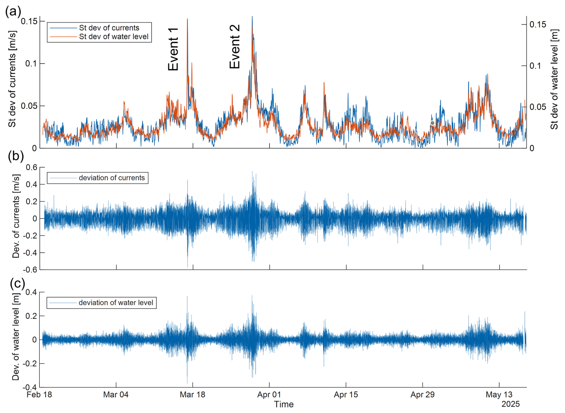
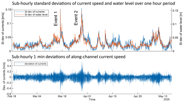
Figure 3 Joint panel of sub-hourly standard deviations of (a) current speed and water level over one-hour period, and the time series of 1 min resolution sub-hourly deviations of (b) along-channel current speed and (c) water level. Labeled are the high-speed cases Event 1 and Event 2.

Currents at Stn. 1 and Stn. 3 were constrained by the flow mainly oriented along the channel. Looking from the lake downstream towards the sea (Fig. 1c), Channel 3 is oriented along 130° (geographical direction of currents) near the lake (Stn. 3) and along 110° near the sea (Stn. 1); landward directions are 310 and 290°, respectively. Near the seashore, at Stn. 1, 38 % of the time the currents had a direction around 110° (± 30°) and 25 % around 310°. At Stn. 3 near the lake, the directions around 190° covered 40 % of the time, and 34 % around 310°. The alongshore currents (Fig. 2d), aligned at 110° at Stn. 1 and 130° at Stn. 3, were rather well correlated, with a Pearson correlation coefficient r ≈ 0.67. Both high-water-level events on 17–18 March and 28 March were associated with landward (negative) along-channel hourly flows up to 0.17 m s⁻¹. At the lakeside Stn. 3, the landward current speed was about 0.04 m s⁻¹ larger than at the seaside Stn. 1. Regarding hourly scalar current speeds, events of higher current speed (up to 0.25 m s⁻¹) were observed coherently at both stations on around 17 and 28 March, and 7 and 11 April, in association with higher wind speeds (Fig. 2b).

3.2 Sub-hourly variability

High-frequency 1 min time series of currents and water levels had a larger variation range than hourly data. Current speed amounted to 0.75 m s⁻¹, compared to 0.25 m s⁻¹ in hourly data. The water level range was 0.27–1.16 m, compared to 0.50–0.91 m for the hourly data. The largest changes were found at Stn. 1 in the seaside part of the channel.

Intensity of sub-hourly variations is described by the standard deviation of sub-hourly values over one-hour intervals (Fig. 3). Average of the sub-hourly standard deviations (background) of scalar current speed and water level, calculated over a 1 h interval, had values of 0.03 m s⁻¹ and 0.03 m, respectively (Fig. 3a). The intensities of along-channel currents and water level (Fig. 3a) as well as the along-channel water-level difference (not shown) were highly correlated (r > 0.85).

Notably, two high-amplitude events were observed, on 16–18 March and on 28–29 March 2025, when a 5-fold increase from the background was found. These events are labeled Event 1 and Event 2 (Fig. 3). Several smaller events occurred, including those on 7 and 11 April.

The sub-hourly water level deviations from their low-passed counterparts had gradually decreasing correlation from sea towards lake: correlation with seaward Stn. 0 decreased from r = 0.74 for seaside Stn. 1 to r = 0.21 for lakeside Stn. 3. While the 1 min-resolution currents at Stn. 1 and Stn. 3 were uncorrelated, their hourly standard deviations were strongly correlated with r = 0.87.

Considering the typical time scale of 10 min for sub-hourly oscillations, given in Fig. 3b and c, the maximum changes (double the oscillation amplitude) in current and sea level – up to 0.8 m s⁻¹ and 0.8 m, respectively – are harmful to ship navigation, harbor operations, and coastal management.

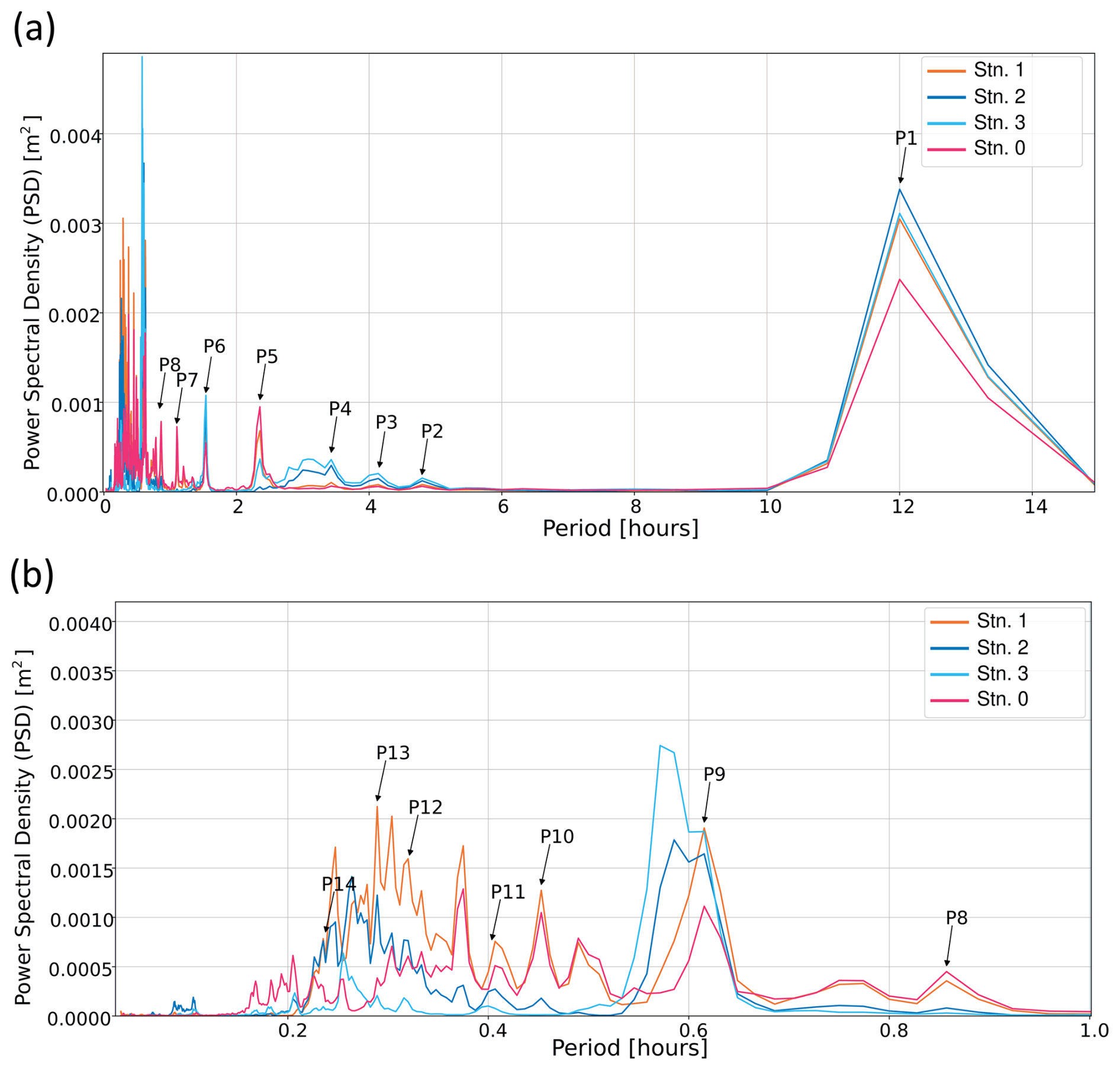
Figure 4 (a) PSD of water level at the four measurement sites of the channel in the range of periods from 2 min to 15 h using a 6 d Welch segment. (b) PSD for periods from 2 min to 1 h, computed using a 1 d Welch segment length to better resolve higher-frequency variability. Marked are the peak periods, starting from the longest period, P1, to the shortest period, P14. Main features of the oscillation peaks are given in Table 2.

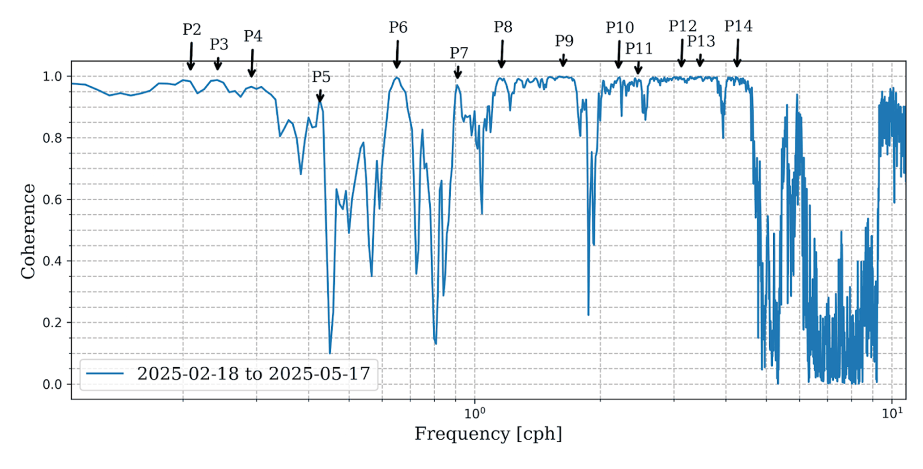
Figure 5 Coherence of water level variability in the channel between Stn. 1 and Stn. 3. The frequency band is from 0.1 to 10 cph (cycle per hour). Marked are the spectral peaks from P2 to P14 shown in Fig. 4.

3.3 Oscillatory analysis

Water level oscillations in the channel were studied using spectral analysis (Fig. 4) and coherence analysis (Fig. 5). Spectral analysis was performed using the Welch method to estimate the power spectral density over a specified frequency range. The basic analysis over a broad frequency range corresponding to periods from 6 min to 14.5 h (Sect. 2.3) revealed that the semidiurnal peak (period about 12 h) had the highest amplitude. This oscillation period is dominant over the whole Black Sea (Medvedev and Kulikov, 2016; Medvedev, 2022) due to tidal forcing. Note that historical spectral estimates lack the high-frequency part of the spectrum due to the 1 h interval of the available observational data.

Table 2 Summary of the spectral analysis of water level time series, with properties of 14 identified spectral peaks. The spectral peaks (given by frequency and period) are characterized by average and maximum intensities in dB and by coherence between Stn. 1 and Stn. 3.

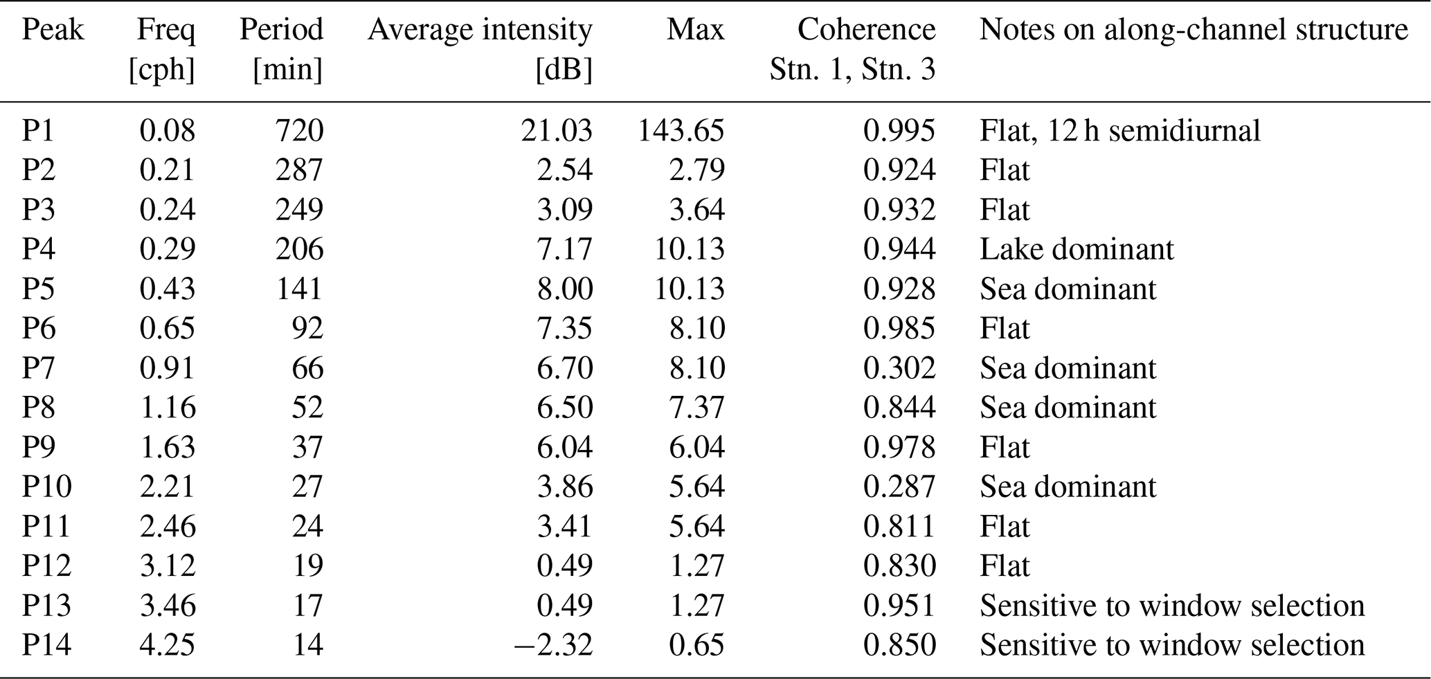
Fourteen spectral peaks, P1–P14, have been identified in the 3-month dataset using the objective procedure described in Sect. 2.3. In contrast, frequency components that were consistently observed across varying Welch window and overlap settings and present at all measurement sites were retained. They are presented in Table 2 and marked in Fig. 4. Among the 14 peaks, determination of 12 longer periods is robust, but 2 shorter periods were somewhat more uncertain, depending on the selection of the calculation window. Most of the frequency peaks were “flat” in space, with the spectral peaks at four locations being nearly equal. Such flat spectral peaks occurred at longer periods, from 12 h (P1) to 4.2 h (P3), at 92 min (P6), at 37 min (P9), and at the shorter periods 24 and 19 min (P11 and P12). Coherence analysis (Fig. 5) revealed high levels for all the identified spectral peaks, meaning nearly synchronous oscillations along the channel. Coherence reduction was evident between the sea-dominant peaks P5 (141 min) and P8 (52 min), but it peaked high again at the flat modes of 92 min (P6) and 66 min (P7). In the shorter periods, reduced coherence became evident between the flat 37 min (P9) and sea-dominant 27 min (P10) modes.

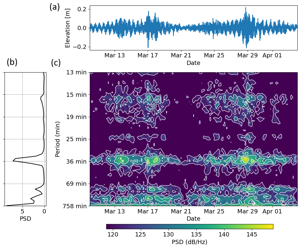
Figure 6 Water level variability at Stn. 1 from 9 March to 5 April 2025 with a 12 h window and 6 h overlap over successive segments. (a) The original data, (b) power spectrum density (PSD) integrated over time, and (c) PSD spectrogram as a function of time and period.

Further insight into the time-dependent character of oscillation amplitudes was gained through spectrogram analysis, which used the short-time Fourier transform (STFT) with a 12 h window and 6 h overlap over successive segments. An example of a spectrogram is given in Fig. 6 based on data from Stn. 1. In the nearly monthly spectrogram, sub-hourly oscillations were concentrated at periods of 36 and 16–17 min (slightly variable in time), corresponding to the peaks P9 and P12–P13 in the 3-month spectra. The oscillations were amplified on 17 and 29 March. These intervals were noted earlier as Event 1 and Event 2 (Sect. 3.2), based on the descriptive graphs of sub-hourly variability (Fig. 3).

The identified 12 “robust” oscillatory peaks P1–P12 and their spatial patterns – flat in four observation stations (7 peaks), sea dominant (4), and lake dominant (1) – will be further analyzed in Sect. 3.5 by interpreting the dominant oscillation patterns using the seiche concept, relying on the approach of barotropic long waves in the channel.

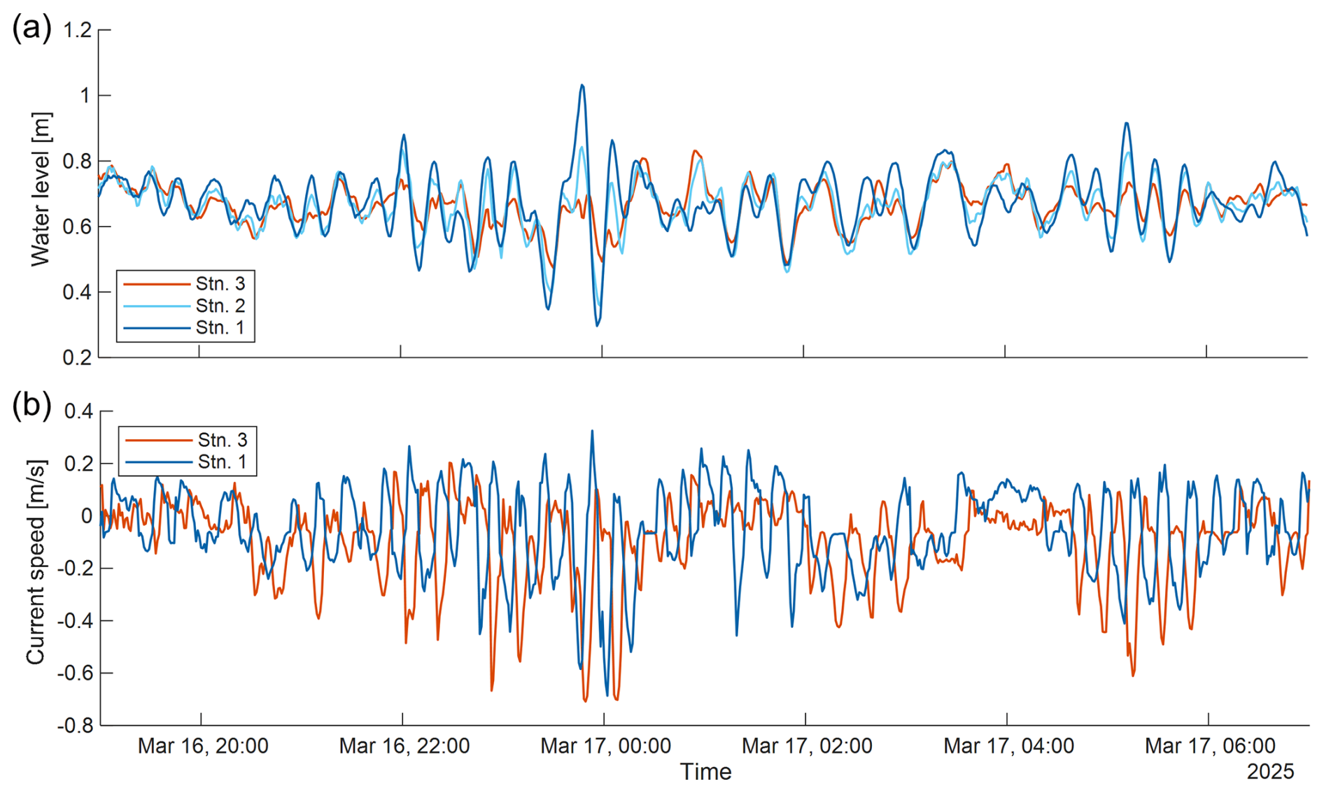
Figure 7 (a) Water level and (b) along-channel current speed during 12 h of the high-current-speed event on 16–17 March 2025. Initial data with a 1 min resolution.

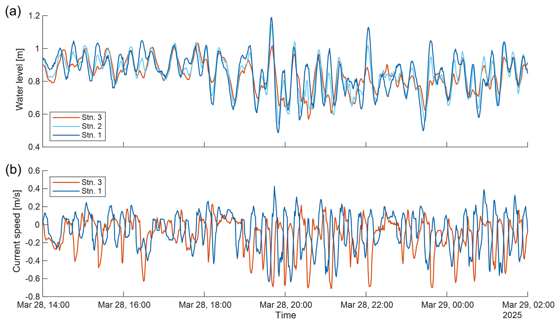
Figure 8 (a) Water level and (b) along-channel current speed during 12 h of the high-current-speed event on 28–29 March 2025. Initial data with a 1 min resolution.

3.4 Analysis of high current speed events

The Events 1 and 2 of high-amplitude water level and current oscillations are visualized by twelve-hour snapshots shown in Figs. 7 and 8, respectively. Correlation of 721 values of 1 min water levels had rather high values of 0.87 inside the channel between Stn. 1 and Stn. 2 for both events; it reduced to 0.53 and 0.61 between seaside and lakeside stations Stn. 1 and Stn. 3, for Events 1 and 2, respectively. The mean periods of most intensive oscillations, measured between sequential maxima and minima, were 18 and 27–40 min for Event 1, and 33–37 and 15–17 min for Event 2. These periods agree with the results from the spectrogram (Fig. 6).

Event 1 was characterized by decreasing westward winds within a diurnal breeze cycle. Regarding possible mechanisms of wind forcing (local, remote, resonant), we note that a short pulse of strong southerly wind occurred 4 d before the event. Just before the highest water level, the zonal wind had a 2 h variation (between consecutive maxima) with an amplitude of 8 m s⁻¹. Shorter period wind speed oscillations were rather weak, less than 1 m s⁻¹. During Event 2, the zonal wind had a westward component with a maximum of −14 m s⁻¹; superimposed variations of 4 m s⁻¹ amplitude had a time scale from 50 to 80 min, shorter-period wind pulsations of 2 m s⁻¹ had a time scale of about 20 min, close to the period of sub-hourly water level oscillations.

During Event 2, wind was variable on a time scale of a few tens of minutes. At the near-lake Stn. 3, water level oscillations were mostly of a 36 min period but were slightly modulated by about a 17 min period. After the peak water level at seaside Stn. 1, the periods changed from 36 to 16–17 min. In Event 1, which had a 2 h zonal wind variation before the water-level maximum, the periods increased from shorter to longer values.

Signal delay from the sea towards the lake was detected in several instances, but statistically, the best correlation for both events was obtained with zero time lag. There was a smaller correlation decay in the case of signal propagation from the sea towards the lake, in comparison to the opposite direction. Event 1 had a more compact water-level maxima pattern than Event 2; it had 8 versus 14 higher local maxima, measured by the 80 % value of the event maximum. Also, the water level standard deviation of Event 1 was about 20 % smaller than that of Event 2.

Along-channel currents of Stn. 1 and Stn. 3 are presented in Figs. 7b and 8b for Events 1 and 2, respectively. In many cases, the current fluctuations at seaside and lakeside locations are out of phase. The current time series, unshifted in time, were uncorrelated in both events; a moderate correlation (0.5–0.6) was observed for time shifts of 16–17 min.

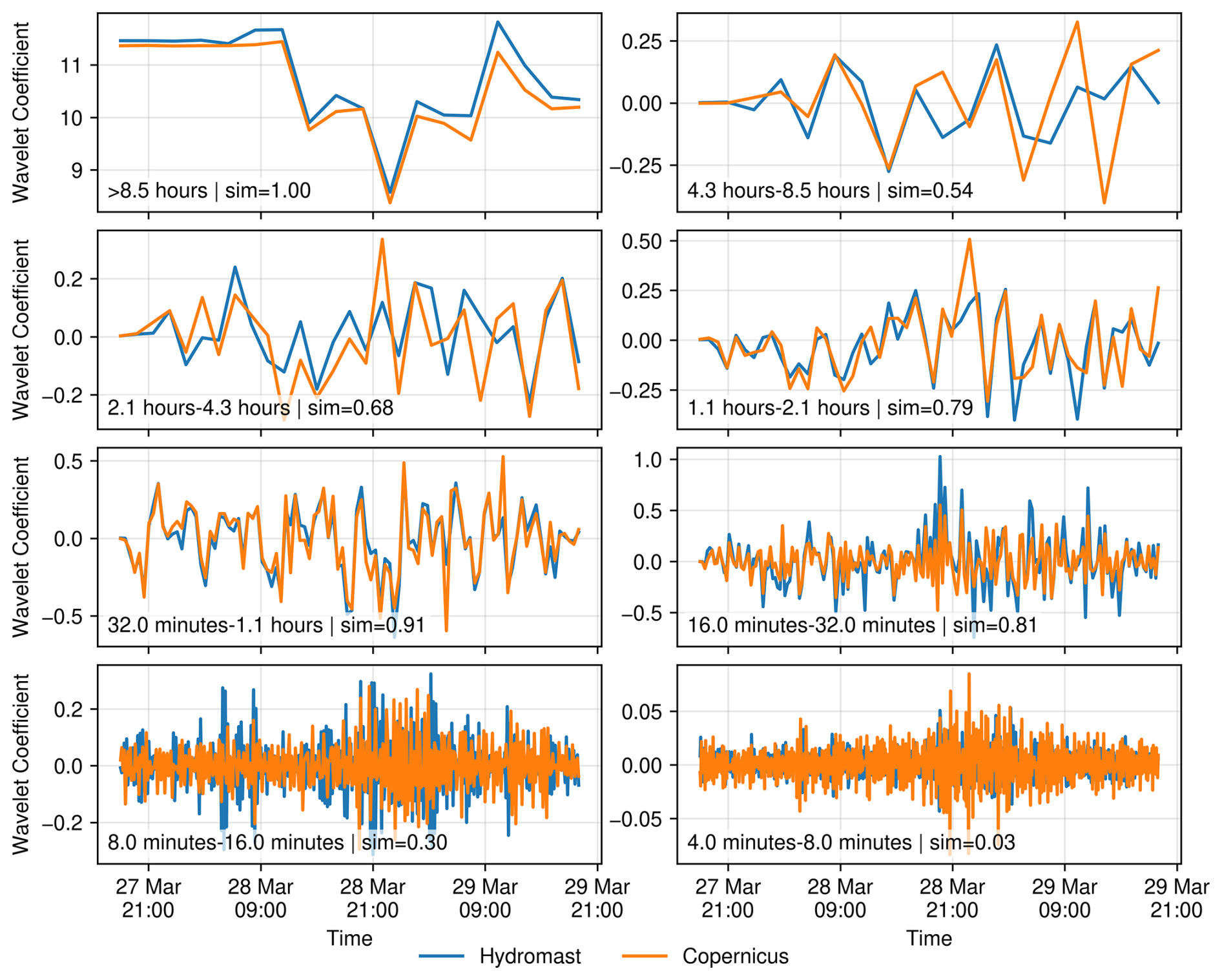
Figure 9 Anatomy of the high-current-speed event from 27 to 29 March, based on 8 frequency bands shown in the sub-figure legends, identified by wavelet analysis. Shown are the results for Stn. 0 (Copernicus) and Stn. 1 (Hydromast), “sim” presents the similarity between the wavelet coefficients in these two stations.

Table 3 Cosine similarity (correlation) of the wavelet amplitudes at Stn. 1 to Stn. 3 with Stn. 0 at different intervals of periods during Event 1 and Event 2.

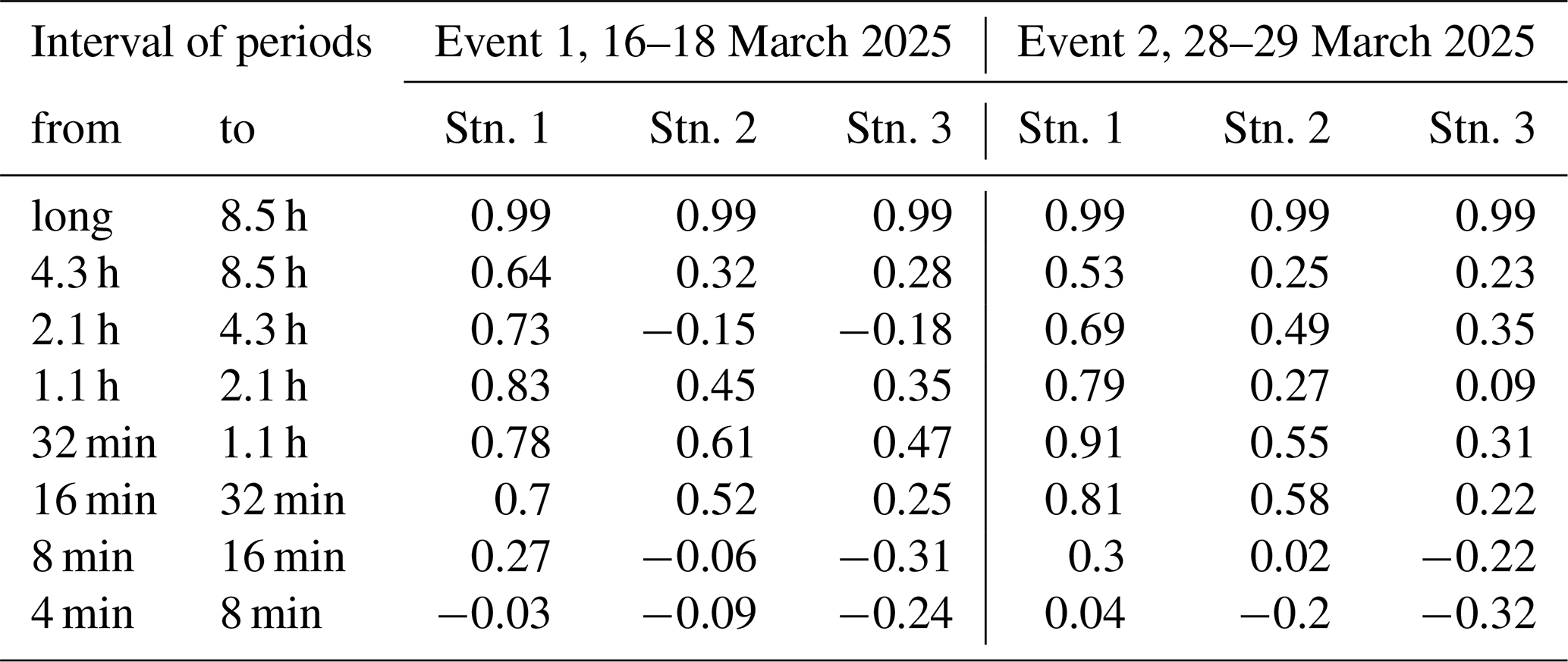
Wavelet analysis was also applied to study water-level oscillations at both events. The wavelet components in different frequency bands are presented in Fig. 9 for the seaward harbor site Stn. 0 and the seaside channel site Stn. 1. Correlations (similarities) between the wavelet component time series of Stn. 0 and all the other three observation sites are summarized in Table 3. At longer periods (more than 8.5 h), all the channel observations showed high similarity (correlation of 0.99) with the data from Stn. 0. The seaside Stn. 1 had high similarity with outside Varna observations at Stn. 0, also in the shorter periods down to 16 min, for both events. The shorter periods from 16 min to 1.1 h covered the resonance periods of long barotropic gravitational waves in a system of a sea-channel-lake (see the next section). At these periods, a higher similarity with Stn. 0 also occurred at Stn. 2, located in the middle of the channel.

Based on the above, Event 1 involved a few high-peak 16–17 min oscillations, observed within about an hour, not directly related to the local meteorological forcing. Such a short pulse is typical of meteotsunamis (Vilibić et al., 2021). Event 2 had a longer duration, involving several oscillations, including also longer 36 min period oscillations, likely generated by short-period (including sub-hourly) meteorological forcing.

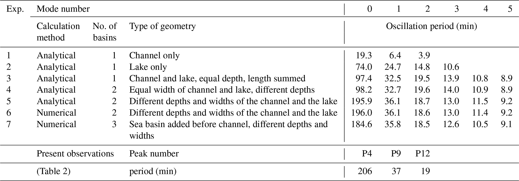
Table 4 Periods of eigenoscillations (seiche) of the first 5 modes, based on 7 experiments with different calculation methods, number of included basins, and type of basin geometry. For comparison, observational peak periods P4, P9, and P12 are taken from Table 2.

3.5 Interpretation of variability by long barotropic waves

The basic question is which hydrodynamic processes cause the observed high-current-speed events. The dynamics of channels and their networks are frequently treated using shallow-water theory, which considers along-channel flow variations averaged over depth and width and employs conservation laws for mass, momentum, and energy expressed as differential equations. A broad spectrum of problems includes flooding and flow routing, long-wave dynamics for transient waves, their reflection, transition, and damping depending on the degree of nonlinearity (e.g., Lighthill and Whitham, 1955). In narrow, elongated basins, where the width is much less than the length, the transverse flow component is damped, thereby decreasing also the influence of Earth's rotation. This results in a 1D model.

In the case of small disturbances of motion from rest (water-level deviations are much smaller than the depth), the flow follows the linear shallow-water equations. For the analytical and numerical solution of the waves, primarily for estimation of the resonant periods, the navigation channels 3 and 1 were approximated by rectangular basins with length L = 2400 m, constant depth H = 7 m, and a total width B = 300 m (merging both of the channels); the lake was approximated with length L = 11 000 m, depth H = 10 m, and width B = 1900 m. The widths are much smaller than the lengths; therefore, the conditions for 1D dynamics are satisfied in the first-order approach for both the channels and the lake. Regarding the assumption of linearity, the observed water-level amplitude up to 0.4 m and current-velocity amplitude up to 0.4 m s⁻¹ over a half-period of 10 min suggest that in the momentum equation the non-linear advection is less than 10 % of the acceleration term. The linear barotropic (with density variations considered small) shallow-water equations (Eq. A1) and related oscillation modes are outlined in Appendix A. Comparison of the “amplitudes” of current speed and water level revealed a ratio consistent with that of long linear barotropic waves, thereby independently justifying the use of a 1D shallow-water approach.

The first interpretations based on quarter-wave resonance used a channel of constant depth, with prescribed water-level oscillations at one end and a closed boundary at the other. Further refinement of the interpretations included a larger study area, idealized as a network of connected 1D channels with small but distinct widths. The two parallel navigation channels (Channels 1 and 3), approximately the same length and depth, were handled in the lake-channel-sea system as a single channel by summing their widths. Note that for a 1D channel, the results are independent of the channel width; width comes into play for connected and/or branching channels, determining transmission and reflection of long waves in individual branches.

Seiche (standing wave) periods were studied using analytical and numerical experiments, labeled Exp. 1 to Exp. 7 (Table 4). Already, the simplest approaches in Exp. 1 and 2 revealed an approximate match to the observed oscillation periods in the range of a few tens of minutes (Table 2). Subsequent refinements from Exp. 3 to Exp. 7 included different configurations of the connected sea, channels, and lake, using analytical and numerical methods. In this interpretation study, detailed consideration of topography and coastline, as well as of non-linear and frictional effects on the flow patterns, was deferred to future studies.

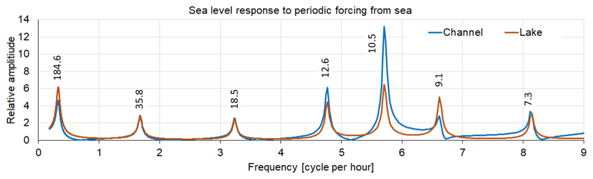
Figure 10 Amplification factor (relative amplitude) of oscillations forced on the seaward side of the channel-lake system with unity amplitude but different periods. Calculations were performed using a numerical time-stepping method with a linear friction coefficient of R = 10⁻⁴ s⁻¹. The resonance periods are 184.6, 35.8, 18.5, 12.6, 10.5, 9.1, and 7.3 min (Table 4, Exp. 7).

Analytical treatment (from Exp. 1 to Exp. 5) of shallow water equations includes, as a special case, the spatial modes (oscillation patterns) depending on the applied boundary conditions. When outer-basin water-level oscillations drive the water level in a channel, the appropriate condition for calculating the spatial modes is to impose a zero water level at the open boundary. The other boundary is considered closed, which makes the velocity zero, equivalent to setting the spatial gradient of the water level to zero. When the basin is “glued” from different parts, with different depths, lengths, and widths, conditions of continuity are applied at the connection point. In the simplest case of one basin of constant depth and width, the “quarter-wave” modes take place as given by Eq. (A2).

Three basic one-basin experiments, Exp. 1 (channel only, forced in the sea, closed at the connection to the lake), Exp. 2 (lake only, forced at the connection to the channel, closed at the western end of the lake, and Exp. 3 (joint channel and lake, mean depth, equal widths, lengths summed) provided self-oscillations (seiche) in the range of periods 13–40 min, involving the observed spectral peaks from 37 min (P9) to 14 min (P14). At Exp. 4 and 5, introducing more details of basin geometries, based on Eqs. (A3) and (A4) did not significantly change the periods of modes from 1 to 5. Sub-experiments with a channel width of 80 m (not shown), corresponding to a single channel 3, revealed approximately the same resonant periods as with merged channels 1 and 3 of total width 300 m. The largest period changes occurred for the longest mode 0 period, which increased with more complex basin configurations, from 98 min in Exp. 3 and 4 to 196 min in Exp. 5, corresponding to the lake-amplified observed peak period P4 of 206 min. These free, frictionless oscillation modes just yield the resonant periods. When variable forcing by water level and/or wind stress is applied, the amplitude of the response oscillations is maximal (local maximum of the amplification factor) when the period of forcing is close to the resonant period.

Modes of standing waves were further studied using time-stepping numerical calculations with the 1D barotropic equations as outlined in the Appendix. The spatial grid step was set to 12 m in the channel and 30 m in the lake, based on sensitivity experiments with different grid sizes. Both basins used a linear friction coefficient of R = 10⁻⁴ s⁻¹ that ensured reasonable amplification coefficients (mostly less than 10) at resonant periods. Using Eq. (A5), the water-level forcing was provided by prescribed oscillations at the seaside boundary. Numerical experiments Exp. 6 and 7 were run over a sufficiently long period (10–30 d) to achieve the regime of persistent forced oscillations. The calculations were conducted over a range of external oscillation periods from 6 to 330 min. For each different oscillation period, 1000 calculation cycles were made. The attainment of oscillations in the persistent pattern was determined using cumulative analyses of peak time series at selected locations. “Steady” oscillations were selected by a backward cycle of the peak heights being within 8 % difference from the cumulative mean peak height. The resulting amplitudes for each forcing period with unity amplitude were collected. The results are presented in Fig. 10, whereas the numerical values of resonant periods are given in Table 4. The origin of each numerically determined resonant period is determined analytically using the mode numbers.

Observations revealed a sea-dominant peak, P5, at 141 min (Table 2), which was absent from the numerically calculated resonant wave excitation periods (Table 4) but is in good agreement with the resonant frequency of the Helmholtz oscillator (Eq. A6). Note that an equal forcing amplitude was used for all calculated periods due to the lack of high-resolution open-sea data; the observed spectra reflect the actual variability in forcing over the broad range of periods.

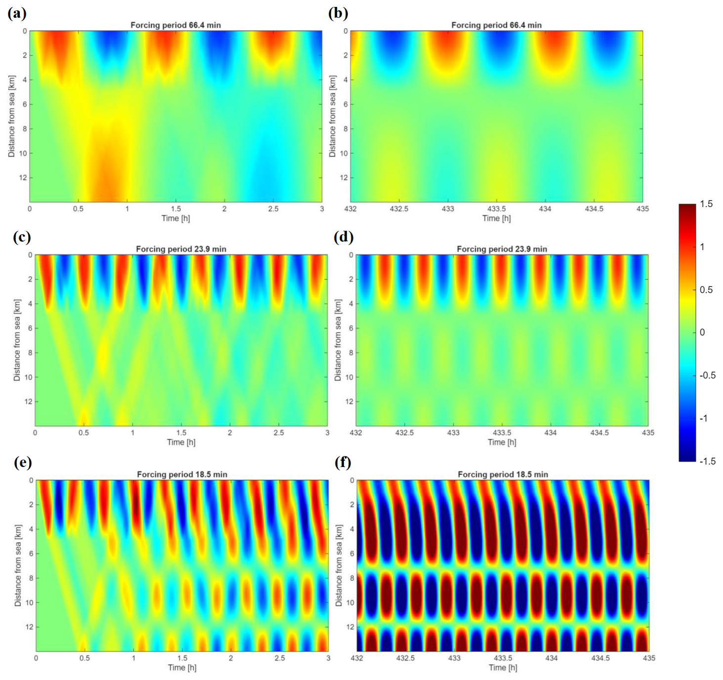
Figure 11 Propagation of sea level oscillations forced on the seaward side of the channel-lake system, with unity amplitude but different periods: 66 min (a, b), 24 min (c, d), and 18.5 min (e, f). Time-distance diagrams cover 3 h during the start of forcing (a, c, e) and during the period of established stationary oscillations (b, d, f). The 300 m-wide channel is connected to a 1900 m-wide lake at the distance of 3 km. The channel has a 600 m-long entrance with a width of 600 m. The color scale “jet” ranges from −1.5 to 1.5.

The high-amplitude events, presented earlier in Sect. 3.4, do not fit the concept of superposition of standing modes with “saturated” amplitudes. Experiments with forced oscillation patterns in the initial and saturated phases are presented in Fig. 11 over three periods. When forcing starts at the seaside of the channel, part of the signal is reflected at the channel-lake junction. Another part, transferred to the lake, accumulates over time until a stationary oscillation pattern is established throughout the channel-lake system. For the oscillation periods of the forcing at 66 min (sea dominant peak P7 in Table 2) and 24 min (flat peak P11), the water-level signal was initially confined within the channel. It did not propagate significantly into the lake from initial (Fig. 11a and b) to the saturated phase (Fig. 11c and d). The numerical setup was adopted from Exp. 7; these periods were found to be peaks in the observations but were not resonant in the numerical calculations (Fig. 10), due to limitations of the model. The third selected period, 18 min, corresponds to the observational “flat” peak P12 and second mode of Exp. 5–7, developed after initial adjustment into the resonant mode covering both the channel and the lake (Figs. 11e and f). Indeed, the pattern in Fig. 11f has two zero crossings, characteristic of the second mode.

Water level changes in the western Black Sea at the coastal stations of Constanta, Varna (Stn. 0), Igne, and Istanbul (Fig. 1) were well correlated during the study period (r = 0.7–0.8) when hourly values from the Copernicus Marine Service were used. However, using hourly data to drive the channel model yielded smooth variations in water level across the hourly values. Sub-hourly forcing data were not available over the larger Varna Bay area, including the adjacent Black Sea stations Igne and Constanta (Fig. 1); therefore, simulation and forecast studies were not conducted.

4 Discussion

4.1 Physics of channel variability

Oscillatory time series from a few points in natural waterbodies are interpreted using wave processes. During resonant forcing of the water level with one or another eigenoscillation period, the initial amplitude growth follows the linear regime used in the present study. In shallow-water Boussinesq equations, at growing amplitudes, non-linear effects, expressed by the cubic non-linearity and quadratic friction, as well as frequency detuning due to finite water-level variation relative to the mean depth, induce slowly evolving subharmonic oscillations of longer periods (Hill, 2003). Assuming the main resonance period in our study was 19 min, the first subharmonic could be 38 min, nearly the same as the observed period. In the pilot study, to interpret the observed sub-hourly water-level and current oscillations, non-linear effects (Teng and Wu, 1992) and variable topography (Valiani and Caleffi, 2024) were not included. For the same reason, full numerical modelling at very high resolution was reserved for future studies.

Sub-hourly current and water-level oscillations have been reported as very important for extreme water levels in the seas with low tidal activity. Recently, Ramos-Alcántara et al. (2025) showed that in the microtidal Mediterranean, sub-hourly periods account for 8 %–24 % of the water-level peak values. At channels and river mouths, this external variability is transferred into coastal embayments, where resonant forcing may occur. In the Klaipeda Strait of the Baltic Sea, which has geometric dimensions comparable to those of the Varna harbor channels, sub-hourly water-level spectral peaks at 14 and 26 min were observed (Nesteckyt$\dot{e}$ et al., 2024). Our study included current observations that are rare in studies of sub-hourly dynamics, which allowed us to demonstrate the long-wave dependence between maximum water levels and currents. However, the main limitation in our study was the lack of sub-hourly forcing data for the identified high-current-speed events.

Meteotsunamis, generated by Proudman resonance of weather patterns moving at the speed of long gravity waves, are well distinguishable in microtidal seas like the Mediterranean and Black Sea (Šepić et al., 2015; Vilibić et al., 2021) and the Baltic Sea (Pellika et al., 2022; Nesteckyt$\dot{e}$ et al., 2024). After the forcing event ceases, oscillations usually decay rapidly. In some cases, seiches persist for long periods (Park et al., 2016). Among the resonance drivers, infragravity waves with periods of 0.5–5 min play a role (Gao et al., 2016). In Varna Bay, with depths up to 20 m, the long-wave phase speed reaches 14 m s⁻¹, which is comparable to the typical speed of cold atmospheric fronts. A review of meteotsunami processes is given by Vilibić et al. (2025).

Another possible short-term forcing comes from wind gusts, including sub-hourly intense air pressure and wind perturbations. For example, intensive wind gusts occur during convective thunderstorms (Mohr et al., 2017). Short-term local atmospheric changes occur due to the passage of fronts (Steinheuer et al., 2025).

It is anticipated that Event 1, presented in the Results section, was generated by a meteotsunami, and a rapid change of weather conditions created Event 2.

4.2 Forecasting high current speed events

The need for sub-hourly resolution in routine meteorological and oceanographic data was recognized as early as the 1950s (Van der Hoven, 1957), who showed spectral peaks in wind data at about 1 min. With the evolution of observation techniques, high-resolution observations have become more widespread, but the dominant data exchange interval in meteorology remains 1 h. In coastal oceanography, water levels are recorded at 1 min intervals in many locations since the 1980s (Miller and Luscher, 2019). Presently, there are initiatives to manage high-resolution water level data, such as SHELDA (Sub-hourly European Quality Controlled Sea Level Dataset; Balić and Šepić, 2025), but standard data exchange for now- and forecasts, such as in Copernicus Marine Service, uses a 1 h resolution.

The hourly gridded data for the Black Sea, generated with a NEMO v3.4 model at 3 km resolution, are already reliable (Ciliberti et al., 2022). In another microtidal waterbody, the Baltic Sea, operational sea-level predictions have reached high performance (Kärnä et al., 2021). Observed sea levels can be extended from the coastal stations to unmonitored coastal and/or offshore locations using the statistical patterns generated from the model results (Elken et al., 2024). Sea level predictions at coastal sites can be fine-tuned using machine learning (Barzandeh et al., 2025).

High-speed current events may be harmful for shipping and harbor operations, but so far, no published operational limits have been identified for the Port of Varna. Navigation restrictions at the port are primarily based on vessel characteristics and environmental conditions, such as wind and visibility, with maneuvering decisions made by the Harbor Master and Traffic Control based on prevailing conditions. Therefore, the observed peak current velocities are reported as hydrodynamic observations rather than compared with fixed operational thresholds.

Prediction of local dynamics, such as flows and water levels, in the Varna Harbor Channels is a typical “downstream” forecast problem, and the following steps should be taken.

• 1.

  Setting up a specific, very-high-resolution model, probably of a shallow-water Boussinesq-equation model.

• 2.

  Creating a parametrization interface, linking the “core” Black Sea data to the local forcing, with a proper description of sub-hourly variability. Implementing machine learning might be useful.

• 3.

  Conducting an extended observation campaign to calibrate and validate the local model's performance.

• 4.

  Running the “downstream” forecast model with a minimum set of observations to fuse the model and observational data at minimal costs.

• 5.

  Disseminate the forecast data, along with “what-if” guidelines for potential harmful situations.

5 Conclusions

Currents and water levels were studied at 1 min resolution in the Varna Port navigation channel, which connects the Black Sea to an upstream lake. While water levels were strongly correlated (r ∼ 0.83–0.94) along the 2.4 km-long channel during a 3-month study period, currents revealed low correlation.

Spectral analysis of the water level identified 14 spectral peaks ranging from 14 min to 12 h. Coherence and wavelet analysis revealed nearly synchronous motions on the periods longer than 14 min; however, coherence was reduced between some of the observed spectral peaks.

Background sub-hourly variability of currents and water levels, with standard deviations of 0.03 m s⁻¹ and 0.03 m, respectively, was occasionally interrupted by events of significantly higher variability. Hourly intensity of sub-hourly variations, quantified by standard deviation, showed strong agreement between water levels and currents (r = 0.86) along the channel. The 2 d events revealed dominant oscillation periods of about 19 and 37 min, resulting in a 5-fold increase in standard deviation compared to the background.

Basic features of high-intensity sub-hourly variations can be interpreted as linear barotropic long waves in a system sea-channel-lake with resonant and damped forcing. The 37 min oscillations can be explained as the first mode of the channel-lake system. Another period of 19 min corresponds to the zero, quarter-wave mode of the channel and the second mode of the channel-lake system.

Events of high current speed can cause changes of 0.8 m s⁻¹ in current velocity and 0.8 m in water level over 10 min, which are sufficient to pose problems for ship navigation, harbor operations, and environmental protection, especially for coastal management and sediment transport.

These high-speed current events can be reliably detected using low-cost observation techniques such as Hydromast, which was used in the present study. Regarding event predictions, the Copernicus Marine Service provides reliable background condition forecasts. The parametrization of the forcing factors for sub-hourly variability – including the effects of meteotsunami generated by moving weather patterns, wind gusts, sub-hourly intense air pressure, and wind perturbations – needs further study to establish their relations with background conditions for the forecast of high-amplitude event occurrence.

Appendix A: Using shallow water equations

Consider long barotropic gravity waves of small amplitude, where the vertical displacement of the water level is much less than the depth of the basin, and the speed of the water particles is significantly lower than the speed of the long waves, within a narrow, elongated basin. The fundamental equations for momentum and volume conservation are outlined in works such as those by Leblond and Mysak (1981) and Cushman-Roisin and Beckers (2011)

$$\begin{array}{}\text{(A1)}& {\displaystyle \frac{\partial u}{\partial t}}=-g{\displaystyle \frac{\partial \mathit{\eta }}{\partial x}}-Ru\text{ and }{\displaystyle \frac{\partial \mathit{\eta }}{\partial t}}=-{\displaystyle \frac{\partial }{\partial x}}\left(Hu\right),\end{array}$$

where u is the current velocity along the basin, η is the water level elevation, H is the depth of the basin, g is the gravity acceleration, and R is linear friction coefficient.

Adopting constant depth, we may search for the solution in the form $u=u_{\mathrm{0}}{e}^{i(kx-\mathit{\omega }t)}$ and $\mathit{\eta }={\mathit{\eta }}_{\mathrm{0}}{e}^{i(kx-\mathit{\omega }t)}$, where k is the along-basin wave number and the frequency $\mathit{\omega }={\mathit{\omega }}_{\mathrm{r}}+i{\mathit{\omega }}_{\mathrm{i}}$ is complex, where the real part ω_r describes the oscillations and the imaginary part ω_i describes their decay in time. The frequency of oscillations is found from the formula ${{\mathit{\omega }}_{\mathrm{r}}}^{\mathrm{2}}=gH{k}^{\mathrm{2}}-R^{\mathrm{2}}/\mathrm{4}$. Oscillatory motions are possible when R < 2ck, where $c=\sqrt{gH}$ is the phase speed of long gravitational waves without friction.

Assume a semi-enclosed basin of length L, forced by oscillations of the water level of the outer large basin $\mathit{\eta }(\mathrm{0},t)={\mathit{\eta }}_{\mathrm{0}}\sin \mathit{\omega }t$, and closed at the other end $u(L,t)=\mathrm{0}$. For the free, frictionless R=0 modes we use $\mathit{\eta }(\mathrm{0},t)=\mathrm{0}$. The closed basin end follows the condition $u_n(L,t)=\mathrm{0}$ that becomes equal to cos k_nL=0 or $k_n=(n+\frac{\mathrm{1}}{\mathrm{2}})\mathit{\pi }/L$. Here n is the mode number of eigenoscillations (seiche mode). Frequencies of all the modes are calculated in the frictionless case in the form

$$\begin{array}{}\text{(A2)}& {\mathit{\omega }}_n={\displaystyle \frac{\sqrt{gH}}{L}}\left(n+{\displaystyle \frac{\mathrm{1}}{\mathrm{2}}}\right)\mathit{\pi }.\end{array}$$

In the basic mode n=0, a quarter wavelength ${\mathit{\lambda }}_{\mathrm{0}}/\mathrm{4}=L$ interpretation is valid (Leblond and Mysak, 1981), where $\mathit{\lambda }=\mathrm{2}\mathit{\pi }/k$. Then the longest period is $T_{\mathrm{0}}=\mathrm{4}L/\sqrt{gH}$.

Elaborate now the approach to the case of two connected basins with different depth, length and width, notated by the indexes 1 and 2. The first basin extends in x∈[0…L₁] and the second one $x\in \left[L_{\mathrm{1}}\mathrm{\dots }\right(L_{\mathrm{1}}+L_{\mathrm{2}}\left)\right]$. A joint standing wave mode has the same frequency, therefore $k_{\mathrm{1}}\sqrt{H_{\mathrm{1}}}=k_{\mathrm{2}}\sqrt{H_{\mathrm{2}}}$. At the connection point of the basins x=L₁, there is continuity of water levels ${\mathit{\eta }}_{\mathrm{1}}(L_{\mathrm{1}},t)={\mathit{\eta }}_{\mathrm{2}}(L_{\mathrm{1}},t)$ and volume transports $H_{\mathrm{1}}{B}_{\mathrm{1}}{u}_{\mathrm{1}}(L_{\mathrm{1}},t)=H_{\mathrm{2}}{B}_{\mathrm{2}}{u}_{\mathrm{2}}(L_{\mathrm{1}},t)$, where B₁ and B₂ are the width of the basins. Let us denote $a=\sqrt{H_{\mathrm{1}}/H_{\mathrm{2}}}$ and $b=B_{\mathrm{1}}/B_{\mathrm{2}}$, then after some mathematical transformations, the wavenumber of the joint mode n in the basin 1 is determined from the implicit equation

$$\begin{array}{}\text{(A3)}& \begin{array}{rl}{k}_{\mathrm{1}}a{L}_{\mathrm{2}}& +{\text{tan}}^{-\mathrm{1}}\left[\text{tan}\right(k_{\mathrm{1}}{L}_{\mathrm{1}})/(ab\left)\right]\\ & -\left(n+m+{\displaystyle \frac{\mathrm{1}}{\mathrm{2}}}\right)\mathit{\pi }=\mathrm{0},\end{array}\end{array}$$

where the number m is to account for the periodicity of the tan⁻¹ function which is selected for each mode n to yield the last continuous intersection point between the growing values of the tan⁻¹ function and k₁L₁. When ab≈ 1, leading to ${\text{tan}}^{-\mathrm{1}}\left[\text{tan}\right(k_{\mathrm{1}}{L}_{\mathrm{1}})/(ab\left)\right]\approx k_{\mathrm{1}}{L}_{\mathrm{1}}$, then the eigenfrequencies are found as

$$\begin{array}{}\text{(A4)}& \mathit{\omega }={\displaystyle \frac{\mathrm{1}}{\mathrm{2}}}{\displaystyle \frac{\sqrt{g{H}_{\mathrm{1}}{H}_{\mathrm{2}}}}{L_{\mathrm{1}}\sqrt{H_{\mathrm{2}}}+L_{\mathrm{2}}\sqrt{H_{\mathrm{1}}}}}\left(n+{\displaystyle \frac{\mathrm{1}}{\mathrm{2}}}\right)\mathit{\pi }.\end{array}$$

When forcing occurs on the resonant seiche period, then in the frictionless case, the amplitudes go to infinity; therefore, friction must be included in the time-series modelling.

To consider the dynamics of the coupled elongated basins (sea-channel-lake) with variable time-dependent forcing, we used a traditional option of 1D numerical equations (e.g., Cushman-Roisin and Beckers, 2011). To capture the effects of variable basin width, the continuity equation (the second equation of Eq. A1) has been rewritten, reaching the equations

$$\begin{array}{}\text{(A5)}& {\displaystyle \frac{\partial u}{\partial t}}=-g{\displaystyle \frac{\partial \mathit{\eta }}{\partial x}}-Ru\text{ and }B{\displaystyle \frac{\partial \mathit{\eta }}{\partial t}}=-{\displaystyle \frac{\partial }{\partial x}}\left(BHu\right).\end{array}$$

In addition to the horizontally resolved motions described by the shallow-water equations (Eqs. A1 and A4), an integrated Helmholtz oscillator approach (e.g., Leblond and Mysak, 1981) was used. The basin with a surface area A is connected to the outer sea by a channel which is considered uniform along the axis. Mean water level of the basin is calculated from the volume flow in the channel. The channel flow is driven by a sea-level difference along the channel length between the forcing external water level and the response water level in the basin. The resonant eigenfrequency is given by

$$\begin{array}{}\text{(A6)}& \mathrm{\Omega }=\sqrt{{\displaystyle \frac{gHB}{AL}}-{\displaystyle \frac{R^{\mathrm{2}}}{\mathrm{4}}}}.\end{array}$$