Thermohaline gradients and frontal regimes in the northwestern Tropical Atlantic

At the edge of the Amazon River plume, stirring by the North Brazil Current (NBC) and its eddies creates sharp surface thermohaline gradients on horizontal scales of 𝒪 (1–100) km. This study provides a comprehensive picture of these gradients and fronts associated with the region's distinctive dynamics. Saildrone observations show that the plume amplifies density gradient variability at all scales from 1–100 km, with frontal sharpness up to 75× stronger inside the plume than outside, with differences reaching 100× at scales below 3 km. Density gradients are partially reinforced or compensated by temperature-salinity variations, with net frontogenesis observed in both regions. To expand in-situ observations, we use a 1 km resolution CROCO (Coastal and Regional Ocean COmmunity model) simulation to assess the spatial distribution of surface fronts and their spatio-temporal variability. We characterize three distinct frontal regimes: (i) broken-up fronts parallel to shore occupy the plume core over the continental shelf, (ii) thin elongated fronts associated with NBC-plume interactions connect nearshore and offshore regions, and (iii) pools of anisotropic fronts driven by the seasonal mixed-layer cycle are present offshore. Salinity dominates density gradients throughout the year north of 15° N, whereas near-shore fronts exhibit seasonal shifts in temperature-salinity dominance linked to the Amazon discharge seasonality and NBC strength. Within the plume, freshwater filaments stirred by NBC rings systematically generate density-compensated fronts on their inner edge and reinforced fronts on their outer rim, a pattern with implications for energy cascades and tracer export.

1 Introduction

The Amazon River reigns absolute as the largest river discharge into the ocean, with an annual average of ∼0.2 Sv (1 Sv=10⁶ m³ s⁻¹) of freshwater entering the northwestern Tropical Atlantic (Perry et al., 1996; Dai and Trenberth, 2002). The offshore propagation of low sea surface salinity (SSS) from the Amazon Plume into the Tropical Atlantic has been observed from drifting buoys and satellite data (e.g., Muller-Karger et al., 1988; Reverdin et al., 2021; Olivier et al., 2024). This propagation is controlled by the seasonality of the Amazon outflow as well as the North Brazil Current (NBC; Flagg et al., 1986; Coles et al., 2013). Influenced by the Amazon Plume, an expanding low-SSS band spreads northwestward in winter and spring (e.g., Reverdin et al., 2021); in summer and fall, the Amazon waters detach from the slope and loop northeastward with the NBC retroflection (e.g., Foltz et al., 2015). As a consequence of the spread of low salinity, a barrier layer driven by Amazon waters occupies a large part of the northwestern Tropical Atlantic (e.g., Masson and Delecluse, 2001; de Boyer Montégut et al., 2007; Romanova et al., 2011), with local and large-scale effects on climate (e.g., Jahfer et al., 2017; Gévaudan et al., 2022; Olivier et al., 2022; Napolitano et al., 2024) and biogeochemical processes (e.g., Weber et al., 2017; Gouveia et al., 2019; Giachini-Tosetto et al., 2022).

The strongest density gradients in the ocean are found at the edge of river plumes (e.g., Wang et al., 2021, and references therein). From 4–20° N, the Amazon water spreads over the shelf break and intersects the warm and salty NBC, with mesoscale and submesoscale dynamics dictating near-surface motions (e.g., Fratantoni and Glickson, 2002; Reverdin et al., 2021). The sharpest gradients at scales ranging from 𝒪 (0.1–100) km (Reverdin et al., 2021; Olivier et al., 2022; Subirade et al., 2023) are generated due to the stirring of the river plume by NBC rings (e.g., Johns et al., 1990; Fratantoni and Glickson, 2002). These submesoscale fronts are important for modulating air–sea interactions (e.g., Strobach et al., 2022), biogeochemical processes (e.g., Freilich et al., 2022), and the energy cascade (e.g., Srinivasan et al., 2023; Zhang et al., 2023b). However, the challenges of observing and simulating small scales have historically hindered the understanding of such complex environments.

In the present study, we use state-of-the-art observations from the EUREC4A-OA campaign and a 1 km resolution numerical simulation to quantify surface thermohaline gradients and characterize frontal regimes in the Amazon Plume region. One objective is to provide a comprehensive picture of the surface gradients and fronts in the Amazon Plume region at different scales. Specifically, we ask: (1) How does the plume modify the scale-dependence and magnitude of density gradients? (2) What is the relative role of temperature and salinity in driving frontogenesis? (3) Do the NBC and its mesoscale dynamics contribute to the spatiotemporal distribution of these fronts? To reach our goals, we revisit in-situ observations from Stevens et al. (2021) and Coadou-Chaventon et al. (2024) to analyze density gradients at fine scales. Then, using outputs from a numerical model, we discuss the spatial distribution of fronts and spatio-temporal control mechanisms.

2 The EUREC4A-OA campaign

Saildrone USVs – Uncrewed Surface Vehicles navigating with near real-time course correction (e.g., Zhang et al., 2019; Farrar et al., 2025) – sampled the ∼1500 km long boulevard de tourbillons region off the Amazon shelf during the EUREC4A-OA campaign (Speich et al., 2021; Stevens et al., 2021, see saildrones' trajectory in Fig. 1a). This eddy corridor connects the South and North Atlantic western boundary currents through the NBC rings, which detach from the NBC retroflection and travel toward the Caribbean Sea (Fig. 1a). In EUREC4A-OA, four of these saildrones were piloted in formation, approximately parallel to each other, equipped with a near-surface Seabird SBE37 Microcat CTD and a 300 kHz RD Instruments ADCP, to adaptively sample across the mesoscale eddies and submesoscale features in this region. The CTD and ADCP were mounted on the saildrones at 0.5 and 2 m below the waterline, respectively. The ADCP first bin was set at 6 m. L'Hégaret et al. (2023) detail the post processing of the EUREC4A-OA Saildrone data, which resulted in 1 min CTD (nominal accuracy of $\pm \mathrm{2}\times {\mathrm{10}}^{-\mathrm{3}}$ °C and $\pm \mathrm{3}\times {\mathrm{10}}^{-\mathrm{3}}$ mS cm⁻¹ for temperature and conductivity, respectively) and 5 min ADCP (±0.5 cm s⁻¹) averages. For additional details on the fleet course and in-situ sampling during the campaign, see Coadou-Chaventon et al. (2024). More on Saildrone instrumentation and observations from different campaigns are available in e.g., Yu (2026) and Bhuyan et al. (2026).

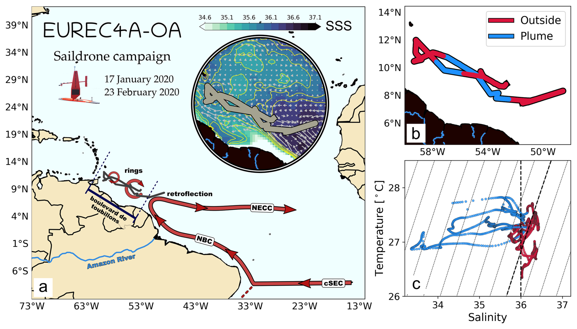
Figure 1 (a) The EUREC4A-OA saildrone campaign (17 January 2020–23 February 2020), with the saildrones' averaged trajectory in gray. The drones navigated the region of the North Brazil Current retroflection and the northwestern-propagating rings. The inset map shows the average sea surface salinity (SSS) from SMAP (Soil Moisture Active Passive mission) during EUREC4A-OA and a blowout of the saildrones trajectory, which (b) sampled regions inside the plume (blue) and outside (red). (c) Temperature–Salinity T–S diagram of the EUREC4A-OA campaign, with colors representing points within the plume (blue) and outside (red). Keys: cSEC: central branch of the South Equatorial Current; NBC: North Brazil Current; NECC: North Equatorial Counter Current.

To compare processes inside and outside the Amazon Plume, we initially derive the position of the plume, bounded by the 36 isohaline, from satellite SSS data (SMAP – Soil Moisture Active Passive mission; Meissner et al., 2022). While other authors use a more conservative approach (; e.g., Molleri et al., 2010; Gévaudan et al., 2022), we choose a wider threshold as in Coadou-Chaventon et al. (2024), which comprises a larger area under the plume influence (e.g., Morozov et al., 2024). We then refine the limits of the plume using the high-resolution saildrone SSS measurements to separate plume and outside (Fig. 1b). This definition leads to a plume similar to that defined in Coadou-Chaventon et al. (2024): our plume region is virtually the same as Coadou-Chaventon's (2024) “Amazon” region, whereas the region outside roughly corresponds to the author's “Upstream” and “Downstream” areas combined. Overall, this definition suffices in isolating the core plume processes from those on the outside, both embedded in warm waters brought by the NBC (Fig. 1c).

3 Observed surface gradients

The along-track measurements obtained by the saildrones provide a multi-scale overview of the surface properties, while drones sailing parallel allow the quantification of 2D gradients. We computed the mean values and gradients simultaneously over a mean trajectory between the four saildrones (see inset in Fig. 1a) from 17 January 2020–23 February 2020. The final resolution of the dataset over the mean trajectory is Δs=1 km (2.5× the saildrones' mean along-track resolution). With data from the four drones, we follow the method in Shcherbina et al. (2013) to obtain temperature (T), salinity (S), horizontal velocities u and v, and their corresponding gradients over this trajectory. Briefly, we gather the measurements of 3–4 saildrones (depending on their mutual distances, on average 2.5±1.0 km) within a moving 8 km$/$120 min-radius circle around the reference trajectory points. The size of the moving circle allows us to avoid temporal variability contaminating the averaged data in each circle, obtaining 138.8±37.9 synoptic measurements (for the saildrones, the synoptic scale is ≃40 km; cf. Coadou-Chaventon et al., 2024) per iteration, i.e., every time the circle moves. At each iteration, we fit a set of linear functions of the form

$$\begin{array}{}\text{(1)}& \mathit{\varphi }={\mathit{\varphi }}_{\mathrm{0}}+{\partial }_x\mathit{\varphi }\left(x-\stackrel{\mathrm{‾}}{x}\right)+{\partial }_y\mathit{\varphi }\left(y-\stackrel{\mathrm{‾}}{y}\right),\end{array}$$

which provide the mean ϕ₀ values, alongside the zonal and meridional gradients ∂_xϕ and ∂_yϕ. We solve Eq. (1) for $\mathit{\varphi }=(u,v,T,S)$ at every point of the mean trajectory by applying a least squares plane fit to all (x,y) observations within the moving circle (cf. Bhuyan et al., 2026). These gradients are gradually smoothed by increasing Δs and the radius of the circle proportionally. Our choice is set for the smallest resolved scale under an accepted error threshold.

Saildrone instrumentation errors are documented in Zhang et al. (2019, 2023a). The uncertainty of observed density gradients could also be affected by e.g., variations in the fleet formation, time lag between drones, and dominant winds over along-current sampling. The choice of the mean trajectory resolution (1 km) and the size of the moving circle (8 km) reduce these and other associated errors, particularly in derived quantities. Still, we estimate the errors of the coefficients in Eq. (1) by calculating the formal least-square uncertainties. For density gradients, we adopt a 95 % confidence interval for temperature and salinity gradients; in other words, we discard gradients smaller than twice their associated error, which removes 7 % of the 1 km-binned data.

3.1 Along-track density gradients

Saildrone along-track density observations allow us to assess the plume influence over multiple length scales through the computation of along-track gradients over a broad range of horizontal scales ℓ. Figure 2 shows, on logarithmic scale, along-track absolute density gradients ∂_ℓρ, subsampled along the mean trajectory of the saildrones from scales between 1 and 100 km ($\mathrm{\ell }=\mathrm{1},\mathrm{2},\mathrm{3},\mathrm{\dots },\mathrm{100}$ km). A histogram counts occurrences per scale of ∂_ℓρ (summing 100 % for each ℓ), where bin values of the gradients can also be translated into a buoyancy frontal sharpness $\mathcal{B}=\frac{\mathrm{1}}{\mathrm{2}}|\mathrm{\nabla }b{|}^{\mathrm{2}}$ (e.g., Gula et al., 2014), with buoyancy $b\equiv -g\frac{\mathit{\rho }}{{\mathit{\rho }}_{\mathrm{0}}}$ (g is the acceleration due to gravity and ρ₀ is the reference mean density). This means, for example, that ${\partial }_{\mathrm{\ell }}\mathit{\rho }\sim \mathrm{5}\times {\mathrm{10}}^{-\mathrm{5}}$ kg m⁻⁴ corresponds to $\mathcal{B}\sim {\mathrm{10}}^{-\mathrm{13}}$ s⁻⁴.

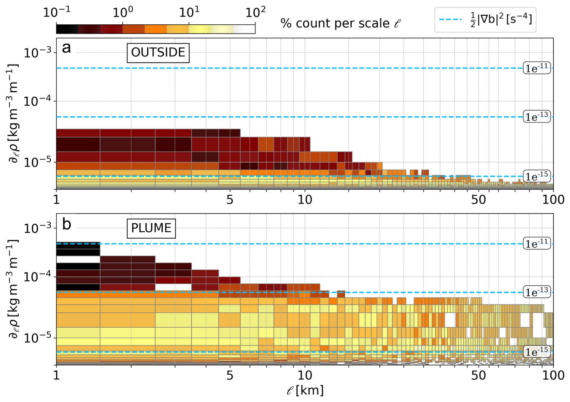
Figure 2 Observed magnitude of surface along-track density gradients per horizontal scale ℓ along the saildrones' trajectory (a) outside and (b) inside the Amazon plume. Colors represent the percentage of gradients for a given scale ℓ (each column sum up to 100 % for every ℓ) and dashed lines represent the buoyancy frontal sharpness ℬ reached for given density gradient thresholds.

Analyzing the saildrone observations from scales between 1 and 100 km reveals that along-track density gradients intensify rapidly when approaching smaller scales, where more sharp buoyancy fronts are present (dashed lines in Fig. 2a and b; also reported by Stevens et al., 2021, using this dataset). These stronger gradients with increasing spatial resolution are consistent with previous numerical simulations (e.g., Molemaker et al., 2015; Balwada et al., 2021). Outside the plume, the strongest density gradients range from $\mathcal{B}=\mathcal{O}\left({\mathrm{10}}^{-\mathrm{14}}\right)$ s⁻⁴ for $\mathrm{1}\le \mathrm{\ell }\le \mathrm{10}$ km, decaying to 𝒪(10⁻¹⁶) s⁻⁴ around ℓ=100 km corresponding to weak large-scale horizontal density gradients (Fig. 2a; see also Whalen and Drushka, 2025, Fig. 3c). This latter value is similar to that of the Johnson et al. (2016) global chart of lateral buoyancy gradients at low-resolution. Within the plume, fronts with $\mathcal{B}\ge \mathcal{O}\left({\mathrm{10}}^{-\mathrm{14}}\right)$ s⁻⁴ are numerous at all scales (Fig. 2b). The fronts reach sharpness values of $\mathcal{B}\ge \mathcal{O}\left({\mathrm{10}}^{-\mathrm{13}}\right)$ s⁻⁴ at 10 km or less, in a combination of strong gradients and small scales, with peaks of ℬ of 𝒪(10⁻¹¹) s⁻⁴ at 1 km (Fig. 2b). Such gradients were reported in very high-resolution numerical simulations (∼150–500 m), which produced fronts as sharp as $\mathcal{B}\sim \mathcal{O}\left({\mathrm{10}}^{-\mathrm{14}}\right)$ s⁻⁴ in the North Atlantic (Srinivasan et al., 2023), $\mathcal{B}\sim \mathcal{O}\left({\mathrm{10}}^{-\mathrm{12}}\right)$ s⁻⁴ in the Gulf Stream (Gula et al., 2014) and even sharper [𝒪(10⁻¹¹)] in the Mississippi River plume (Barkan et al., 2017a, 2019).

Considering the 10 % strongest fronts, ℬ is on average 75× stronger within the plume than in the outside. The largest differences (up to 100×) occur at small scales (). Besides their difference in magnitude, the variance of the buoyancy sharpness increases toward smaller scales both outside and within the plume (see Appendix A). The ℬ variance outside increases linearly from 10⁻³¹ s⁻⁸ at ℓ=50 km to 10⁻²⁸ s⁻⁸ at ℓ=5 km. In the plume, the ℬ variance grows abruptly for ℓ≤10 km, from 10⁻²⁸ s⁻⁸ to about 10⁻²³ s⁻⁸ at ℓ=1 km.

This shift between the two regions suggests that frontogenesis driven by ageostrophic motions may be amplified by density gradients within the plume; such processes display high-vorticity and strain and are related to a recently observed shift from an inverse to a direct energy cascade on scales smaller than 10 km (cf. Balwada et al., 2022, although not independent from seasonality and location). We remind that, at large scales (≥50 km), results should be interpreted with caution, since the effects of temporal variability are non-negligible for ℓ≳40 km (i.e., the local synoptic scale; Coadou-Chaventon et al., 2024). The accuracy of the results could also be impacted by the direction in which the saildrones cross the fronts and changes in the fleet route, which are not considered in this study.

Having established that the plume dramatically amplifies density gradients, particularly at scales below 10 km, we now examine the respective roles of temperature and salinity gradients in setting up density gradients through frontogenesis, and how temperature–salinity (T–S) relations act to partially compensate or reinforce the density gradients.

3.2 Compensation, reinforcement, and frontogenetic tendency

A density gradient may be dominated by a temperature or a salinity gradient. Furthermore, both may combine to reinforce the density gradient or otherwise compensate each other to reduce it (cf. Stommel, 1993; Ferrari and Rudnick, 2000). The relation between these T–S gradients can be quantified by the Turner angle

$$\begin{array}{}\text{(2)}& \text{Tu}=\arctan \left(\mathcal{R}\right),\end{array}$$

which replaces the infinite scale of the density ratio

$$\begin{array}{}\text{(3)}& \mathcal{R}={\displaystyle \frac{\mathit{\alpha }\mathrm{\Delta }T}{\mathit{\beta }\mathrm{\Delta }S}},\end{array}$$

by a finite one (Ferrari and Rudnick, 2000). The density ratio in Eq. (3) evaluates the combined effect of the variation of temperature (ΔT) and salinity (ΔS) on density gradients, where α and β are the thermal expansion and haline contraction coefficients, respectively. This ratio is positive (negative) for compensated (reinforced) gradients, with $\text{Tu}=\mathit{\pi }/\mathrm{4}$ (ℛ=1) representing fully compensated gradients. The Turner angle has recently been used to assess the effect of large freshwater discharges on oceanic density gradients (e.g., Barkan et al., 2017b; Spiro-Jaeger and Mahadevan, 2018; Drushka et al., 2019; Duan et al., 2024). In the present work, we compute Tu for the T–S gradients within 95 % confidence interval (see Sect. 3).

Regardless of their T–S origin, the sharpening of buoyancy gradients indicates frontogenesis (McWilliams et al., 2019; McWilliams, 2021). The weakening of such fronts indicates frontolysis. McWilliams et al. (2019) derived the advective frontogenetic tendency for buoyancy,

$$\begin{array}{}\text{(4)}& {\mathit{\tau }}^{\mathrm{b}}=-\left({\partial }_i{b}^{\prime }\right)\left({\partial }_i{u}^j\right)\left({\partial }_j{b}^{\prime }\right)-\left({\partial }_i{b}^{\prime }\right)\left({\partial }_{i}w\right)\left({\partial }_{z}b\right),\end{array}$$

in which the compact index notation (i,j) span (x,y), with the horizontal velocity $u^{(x,y)}=(u,v)$ and horizontal derivatives indicated by $({\partial }_x,{\partial }_y)$. Since we only have surface buoyancy from the saildrones, the vertical derivative ∂_zb is neglected, as is the second term on the right hand side of Eq. (4), where w is the vertical velocity. The equation thus reduces to the horizontal advective frontogenetic tendency, with buoyancy anomaly b^′,

$$\begin{array}{}\text{(5)}& {\mathit{\tau }}^{\mathrm{b}}=-\left({\partial }_i{b}^{\prime }\right)\left({\partial }_i{u}^j\right)\left({\partial }_j{b}^{\prime }\right),\end{array}$$

which is the leading order term of Eq. (4) (Barkan et al., 2019). We consider both CTD-derived buoyancy values at 0.5 m and ADCP velocities at 6 m as surface measurements.

To estimate errors of the frontogenetic tendency, we first obtain the uncertainties of velocity and buoyancy gradients prescribing an uncorrelated and homogeneous error of ϵ=0.025 m s⁻¹ (u and v; Bhuyan et al., 2026) and $\mathit{ϵ}=\mathrm{7}\times {\mathrm{10}}^{-\mathrm{6}}$ s⁻² (the mean standard error of b^′) for the saildrones. Adding the errors to Eq. (5), we apply basic rules for error propagation of multiplication and powers and normalize by the values of the corresponding gradients. The relative error

$$\begin{array}{}\text{(6)}& \mathit{\sigma }\left({\mathit{\tau }}^{\mathrm{b}}\right)=\mathrm{2}\mathit{\sigma }\left({\partial }_i{b}^{\prime }\right)+\mathit{\sigma }\left({\partial }_i{u}^j\right),\end{array}$$

with $\mathit{\sigma }\left(\mathit{\varphi }\right)=\frac{{\mathit{\varphi }}_{\text{err}}}{\mathit{\varphi }}$, must be smaller than a threshold σ_max. Since calculating τ^b involves multiple derivatives, we accept errors equivalent to 20 % of the inertial (f) and buoyancy (N²) frequencies, for velocity and buoyancy gradients, respectively. We calculate f at each point of the trajectory and obtain an average N² for plume and outside from shipboard in-situ data during the EUREC4A-OA campaign (L'Hégaret et al., 2023). The maximum error in Eq. (6) becomes

$$\begin{array}{}\text{(7)}& {\mathit{\sigma }}_{max}=\mathrm{2}\left({\displaystyle \frac{\mathrm{0.2}{N}^{\mathrm{2}}}{{\partial }_i{b}^{\prime }}}\right)+{\displaystyle \frac{\mathrm{0.2}f}{{\partial }_i{u}^j}}.\end{array}$$

After removing samples with errors larger than σ_max (Eq. 7), we keep 93 % of the Tu and 91 % of τ^b. Combining both, we build Fig. 3 using 88 % of samples at 1 km.

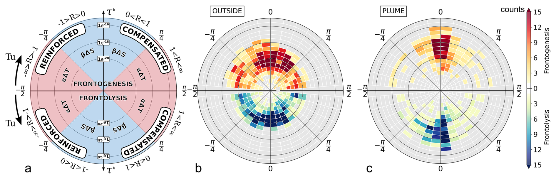
Figure 3 Overview of observed gradients. (a) Schematic diagram mirroring gradients related to frontogenesis (top) and frontolysis (bottom). Radial distances represent the strength of τ^b [s⁻⁵]. Azimuthal distances represent Turner angle Tu (clockwise from $\frac{-\mathit{\pi }}{\mathrm{2}}$ for frontogenesis and counterclockwise for frontolysis), where quadrants indicate if density gradients are driven by salinity (blue) or temperature (red) and if they compensate or reinforce each other. (b, c) Saildrone surface density variations at ℓ=1.0 km scale outside (b; 1964 samples) and inside the plume (c; 810 samples). Colors indicate the number of gradients sampled for each azimuthal and radial bin.

Breaking down the density gradients observed at 1 km reveals the role of temperature and salinity in their composition. We group the gradients along $\text{Tu}]\frac{\mathit{\pi }}{\mathrm{2}};\frac{\mathit{\pi }}{\mathrm{2}}[$ and $\left|{\mathit{\tau }}^{\mathrm{b}}\right|$ [0–10⁻¹⁵ s⁻⁵], separating gradients undergoing frontogenesis and frontolysis. Finally, we add up their occurrences (counts) to present a comprehensive picture of the observed gradients in Fig. 3.

Overall, frontogenesis is partially mirrored by frontolysis (Fig. 3b and c). Nevertheless, our observations hint at net frontogenesis driven by the strongest τ^b, with maximum values of 𝒪(10⁻¹⁸) s⁻⁵ outside and 𝒪(10⁻¹⁶) s⁻⁵ within the plume. Outside, the ∼2000 observed buoyancy gradients typically show ${\mathit{\tau }}^{\mathrm{b}}\le \mathcal{O}\left({\mathrm{10}}^{-\mathrm{19}}\right)$ s⁻⁵, with temperature- and salinity-dominated gradients distributed throughout the range of Tu (Fig. 3b). At large-scales, Whalen and Drushka (2025) showed strong salinity influence over all the northwestern Tropical Atlantic. The higher occurrence of salinity dominance ($-\mathit{\pi }/\mathrm{4}<\text{Tu}<\mathit{\pi }/\mathrm{4}$; see Fig. 3a), even in the region outside, is likely due to a remnant plume from previous seasons (e.g., Muller-Karger et al., 1988; Coles et al., 2013; Fournier et al., 2017).

Mixed-layer instabilities and atmospheric forcing also play a role generating submesoscale fronts across the whole domain; locally, we assume that the NBC and the plume's influence are strong enough to intensify or reduce these effects significantly (e.g., Coles et al., 2013). For example, in Fig. 3, the co-occurrence of frontolysis and frontogenesis hints at a pattern typical of arched flows, with a confluent region followed by a diffluent one (e.g., McWilliams et al., 2019). While only a handful of relatively strong gradients ${\mathit{\tau }}^{\mathrm{b}}\ge \left|{\mathrm{10}}^{-\mathrm{18}}\right|$ s⁻⁵ are associated with frontogenesis outside, (Fig. 3b), they become 𝒪(10⁻¹⁶) within the plume (Fig. 3c). Not surprisingly, salinity gradients are largely dominant within the plume, and the distribution around ℛ∼0 highlights the large difference between the magnitude of temperature and salinity gradients. At 1 km, τ^b that reaches $\mathcal{O}\left|{\mathrm{10}}^{-\mathrm{16}}\right|$ s⁻⁵ is comparable to (model) values in the Mississippi River plume (Barkan et al., 2017b, 2019, Δx∼500 m resolution) and in energetic Gulf Stream meanders (McWilliams et al., 2019, Δx=1.5 km).

In the salinity-dominated Bay of Bengal, Spiro-Jaeger and Mahadevan (2018) observations showed a shift from ℛ=0 at 100 km scales towards compensated fronts at 1 km scale, attributing the compensation effect to the surface cooling of salinity dominated gradients at submesoscale. Within the Amazon Plume, Coadou-Chaventon et al. (2024) found partially compensated T–S gradients dominant at different scales in the 20 % highest scale coefficients αΔT and βΔS. Taking every gradient at ℓ=1 km, the y-axis symmetry shows that partial reinforcement occurs almost as much as partial compensation (Fig. 3b and c), and temperature-dominated gradients partially compensated by salinity (ℛ∼2), appear mostly outside (Fig. 3b). Such partial compensation is ubiquitous in the global ocean (e.g., Rudnick and Martin, 2002). Both within the plume and outside, observations also capture robust compensation (ℛ≃1), although less often (Fig. 3b and c). To this point, our data allow us to only infer, based on the dynamics of the region, that this pattern could arise from the equatorial-warm NBC pushing fresh river water inbound the cooler and saltier Tropical Atlantic, creating freshwater filaments in a background of rather uniform temperature gradient. Such filaments present compensation on the warmer side of the filament and reinforcement on the colder one (see e.g., Duan et al., 2024, Fig. 8f for a cold filament with the same consequences for Tu).

When comparing statistics of observed frontogenesis, frontolysis, and Tu, matching probability density functions (pdfs) for frontogenesis and frontolysis with skewness ∼0 and kurtosis <0 show no predominance between T and S nor between compensation and reinforcement outside (Fig. 4a). High positive kurtosis within the plume further supports compensated and reinforced fronts heavily dominated by salinity (Fig. 4b). Although modest, negative skewness points to slightly more compensation, becoming particularly important for fronts undergoing frontogenesis within the plume.

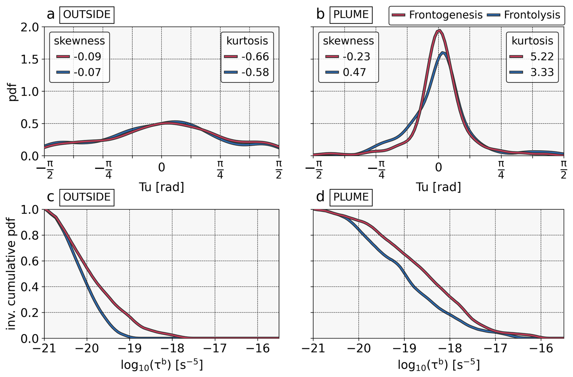
Figure 4 Statistics of observed Tu and τ^b at ℓ=1 km. (a, b) Pdf of Tu separated between gradients showing frontogenesis (red) and frontolysis (blue), for (a) outside and (b) the plume. (c, d) Inverse cumulative pdf of frontogenesis (red) and frontolysis (blue) for (c) outside and (d) the plume.

There is a systematic predominance of frontogenesis over frontolysis in the range $\mathcal{O}\left|{\mathrm{10}}^{-\mathrm{20}}\right|<{\mathit{\tau }}^{\mathrm{b}}<\mathcal{O}\left|{\mathrm{10}}^{-\mathrm{18}}\right|$ s⁻⁵, with up to more than 20 % of the gradients undergoing frontogenesis than frontolysis (Fig. 4c and d). This persistent excess of frontogenesis over frontolysis implies that the region is not simply redistributing existing gradients, but actively sharpening them. Extreme τ^b observed within the plume likely drives convergent downwelling and subduction of surface tracers into the pycnocline (e.g., Capó et al., 2021; Pham et al., 2024).

Finally, the larger-than-expected ratio of reinforced fronts in the current analysis can be explained by

• the evaluation of near-surface gradients compared to deeper gradients (e.g., Ferrari and Rudnick, 2000), where unstable gradients are more likely to occur;

• the use of every sampled gradient instead of a specific section (e.g., Spiro-Jaeger and Mahadevan, 2018) or a selection of a few % strong gradients (e.g., Coadou-Chaventon et al., 2024), where a bias can be introduced due to reinforced gradients becoming unstable and usually not producing T–S gradients as sharp as in compensated fronts (e.g., Duan et al., 2024); and

• the local dynamics driven by the interaction of the Amazon Plume and the NBC, which we discuss in more details later in this study.

So far, we have shown that density gradients intensify within the Amazon plume, especially at scales ≤10 km. There, fronts are salinity-dominated and partially compensated or reinforced by temperature, with local dynamics acting to sharpen them, resulting in net frontogenesis. Outside the plume, T–S gradients are weaker and more uniformly distributed in the Tu−τ^b space, suggesting a competition between a remnant salinity-dominated surface layer and temperature fluctuations brought about by the seasonality of the NBC and local dynamics.

In the next section, we further explore gradients in the Amazon plume region using a numerical simulation to explore their spatial and temporal variability.

4 The numerical model

The model is CROCO (Coastal and Regional Ocean COmmunity model, based on the Regional Oceanic Modeling System; Shchepetkin and McWilliams, 2005). The simulation belongs to the GIGATL family (Gula et al., 2021, hereafter GIGATL1) over the Atlantic Ocean with a nominal horizontal resolution of 1 km and 100 terrain-following vertical levels. The simulation uses hourly CFSR (Climate Forecast System Reanalysis; Saha et al., 2010) atmospheric forcing, a turbulence closure scheme (Umlauf and Burchard, 2003) for parameterization of vertical mixing, and SRTM30plus bathymetry (Becker et al., 2009). The Amazon River input is a monthly climatology from Dai and Trenberth (2002). Barotropic tidal forcing at the boundaries and tidal potential and self attraction are from TPXO7.2 and GOT99.2b. Boundary conditions are from SODA (Simple Ocean Data Assimilation; Carton and Giese, 2008). GIGATL1 is initialized in July 2007 from the 3 km simulation GIGATL3, which was in turn initialized with SODA in January 2004. GIGATL1 and GIGATL3 share the same configuration except for the horizontal resolution and initial condition. We draw snapshots and time series from 20 months of hourly surface output from the simulated years 2008 and 2009.

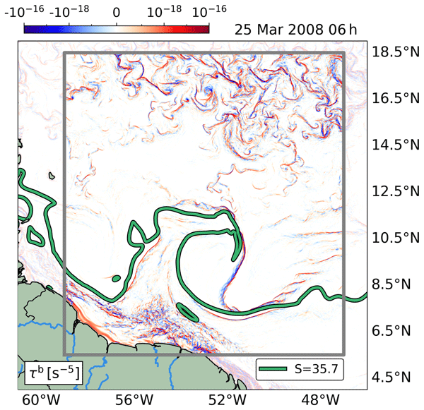
We first analyze a model snapshot exhibiting characteristics similar to those observed during the EUREC4A-OA campaign. The modeled plume on 25 March 2008, 6 h partially occupies the 59–47° W, 4.5–15° N region where we conduct our analyses (Fig. 5a). The chosen snapshot also captures the NBC retroflection next to the plume, a scenario depicted from satellite data during the campaign (see inset map in Fig. 1a and Fig. 1 from Coadou-Chaventon et al., 2024). The choice of a single snapshot to sample the plume and outside comes from the idea of minimizing plume-related processes being captured outside and vice-versa, since we use a simple salinity criterion to separate the regions. Rather than obtaining a direct comparison with the campaign (the modeled plume lags one month behind observations; see Appendix B), our focus is to show that the model is able to represent density gradients and T–S relations similar to the observations.

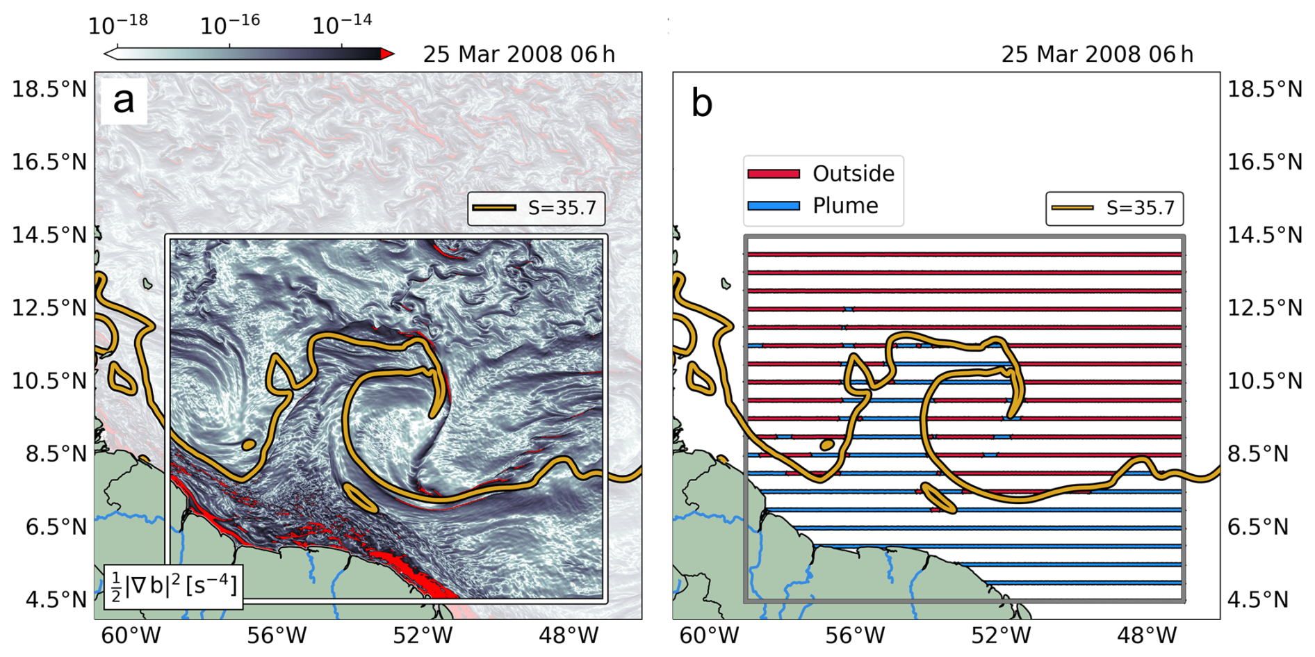
Figure 5 (a) Model spatial distribution of buoyancy sharpness $\mathcal{B}=\frac{\mathrm{1}}{\mathrm{2}}|\mathrm{\nabla }b{|}^{\mathrm{2}}$ and the separation between plume and outside regions using the 0.25 quantile of the salinity distribution. (b) Latitudinal transects used to compute the magnitude of surface density gradients within the plume and outside.

As for the observations, we start by comparing 1-D density differences along multiple zonal transects within the plume and outside, taken at 0.5° longitude and latitude intervals within the 59–47° W; 4.5–14.5° N region (Fig. 5b). However, contrary to observations, in the model we adopt a varying salinity threshold to define the plume: the 0.25 quantile – one-fourth of the SSS probability distribution, hereafter 𝒬₂₅ – which separates the strongest SSS gradients of the plume from the outside (see Appendix C). This moving threshold helps to capture the plume over a longer period than in the observations, while preserving its seasonal cycle.

The model reproduces the key observational signatures: stronger and more variable density gradients within the plume than outside, salinity dominance of fronts, and net frontogenesis both within the plume and outside. The main limitation is that the contrast between both regions is less pronounced in the simulation, owing to the model's effective resolution smoothing the sharpest submesoscale gradients and blurring the plume boundary. Keeping this in mind, we benefit from the model's spatial and temporal coverage to interpret the dynamical mechanisms behind the observed frontal characteristics.

Our detailed model analyses below begins by focusing on comparisons with observations collected by the saildrones.

4.1 Modeled density gradients

Initially, we restrict our analysis and comparisons to a region similar to the one sampled by the saildrones, where the Amazon Plume and NBC are present (Fig. 5a). On 25 March, a freshwater tongue penetrated the open ocean to the northwest, with a retroflecting NBC dragging low salinity (S<35.7) to the northeast (Fig. 5a; see also Fig. C3 in Appendix C). Strong ℬ occur within the plume along the continental shelf and over the recirculating branch of the NBC. Patches of strong ℬ stretch from the shelf, surrounding eddies and marking filaments on the path of the NBC retroflection. In the region outside, some strong ℬ detach from the plume and enter a second dynamical regime that extends from ∼14° N to the northern portion of the domain, away from the direct influence of the NBC.

With transects defined in Fig. 5b, the per scale distributions in Fig. 6a and b display plume and outside points from our snapshot. The modeled ∂_ℓρ and associated ℬ are consistent with saildrone observations, with the model capturing extreme values in the same range as the observations. The model variability is also greater within the plume across the scales, even though differences are less striking than those reported by saildrone data. We attribute the weaker contrast between the two simulated regions to unresolved ageostrophic flows due to the model's horizontal resolution (partially resolving submesoscales in low latitudes), which hinders the divergent strain field directly related to submesoscale frontogenesis (Barkan et al., 2019). Additionally, model diffusion acting at scales up to the effective resolution of the model will likely smooth the sharpest gradients, consequently clouding the limits between plume and outside. Nevertheless, ℬ values in Fig. 6b have been reported in other regions by previous regional modeling studies with at least twice the resolution (e.g., Gula et al., 2014; Barkan et al., 2019), attesting to the unparalleled strength of gradients around river plumes (e.g., Wang et al., 2021).

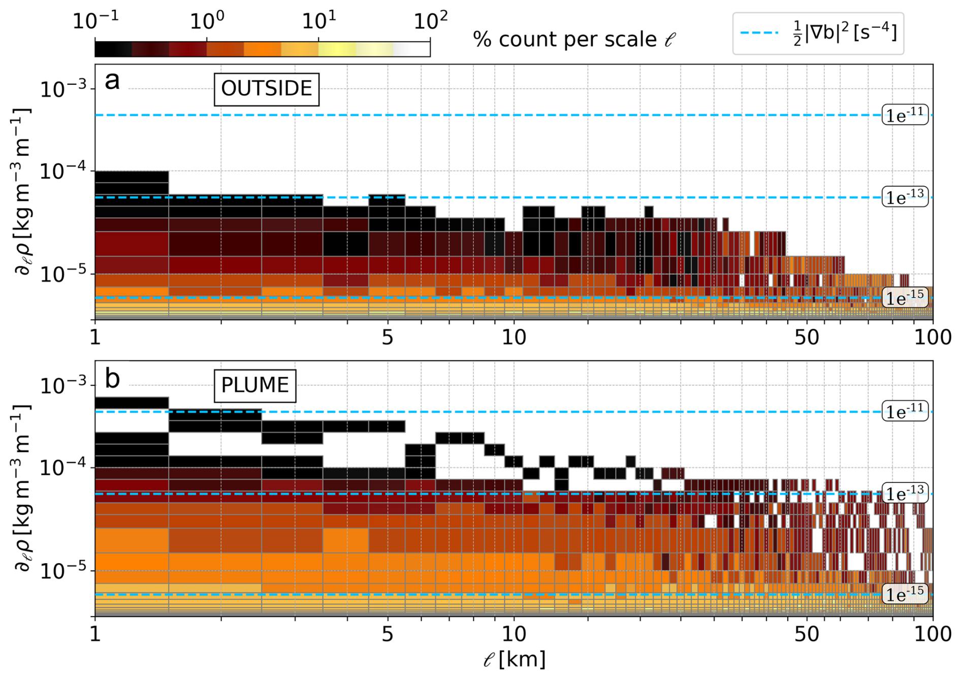
Figure 6 Magnitude of modeled surface density gradients, along latitudinal transects and per horizontal scale ℓ, outside (a) and inside the Amazon plume (b). Colors represent the percentage of gradients for a given scale ℓ (each column sum up to 100 % for every ℓ) and dashed lines represent the buoyancy frontal sharpness ℬ reached for given density gradient thresholds.

4.2 Compensation, reinforcement, and frontogenetic tendency in the model

From model outputs, we computed Tu using the two-dimensional horizontal temperature and salinity variations ΔT and ΔS. For τ^b, we decided to use the “horizontal” definition in Eq. (5) to constrain the analysis to the surface, which allows a (more) direct comparison with observations.

The representation of gradients in Tu−τ^b space (Fig. 7a) confirms the signature of both temperature and salinity outside (Fig. 7b). The role of the Amazon Plume stands out by driving intense frontogenesis within salinity-dominated gradients (Fig. 7c; e.g., Liu et al., 2026). The separation between plume and outside in the model is not as extreme as in the observations, because smoothed gradients struggle to set the boundaries that separate the two regions. The model also encompasses every gradient in one region, notably displaying more temperature-dominated gradients within the plume compared to observations (Fig. 7c). These gradients are mainly associated with the NBC (more on Sect. 5) and were virtually absent in the observations during the EUREC4A-OA campaign (Figs. 2b and 3c), but could be present in distinct saildrone trajectories on the outskirts of the plume. Still, the strongest frontogenetic gradients occur in the plume, heavily dominated by salinity.

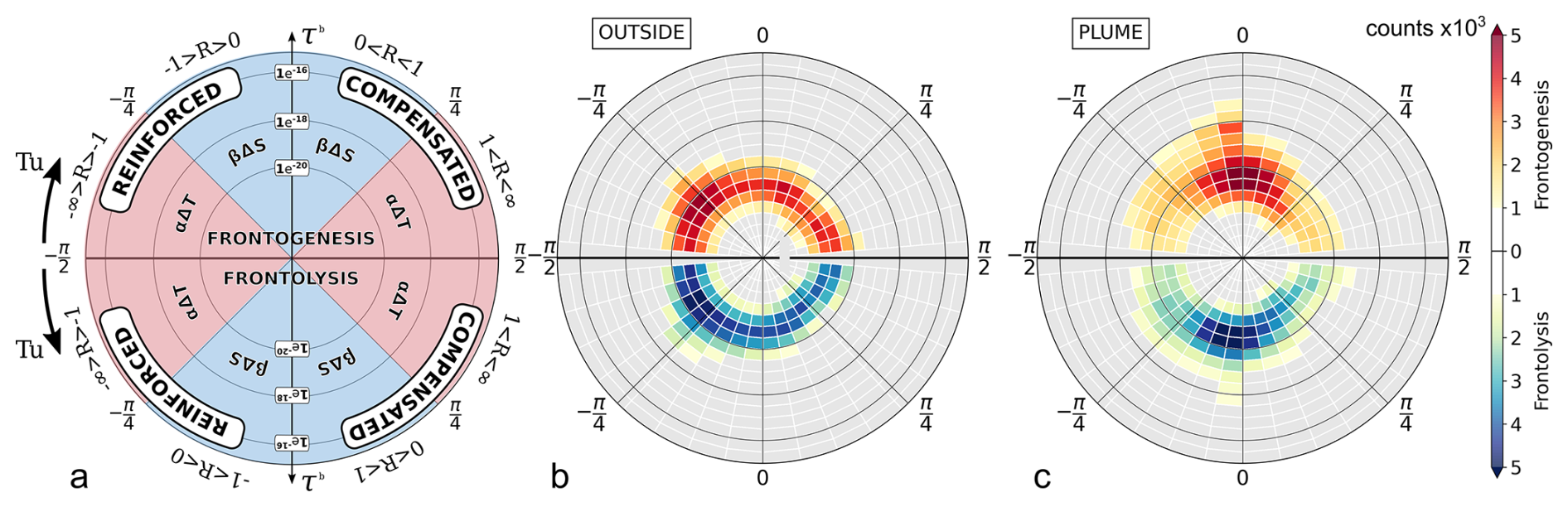
Figure 7 Overview of modeled gradients. (a) Schematic diagram mirroring gradients related to frontogenesis (top) and frontolysis (bottom). Radial distances represent the strength of τ^b. Azimuthal distances represent Turner angle Tu (clockwise from $\frac{-\mathit{\pi }}{\mathrm{2}}$ for frontogenesis and counterclockwise for frontolysis), where quadrants indicate if density gradients are driven by salinity (blue) or temperature (red) and if they compensate or reinforce each other. (b, c) Modeled surface density variations at ℓ=1.0 km scale outside (b; 471276 samples) and inside the plume (c; 472332 samples); the region outside was randomly subsampled so the colorbar scale matches both regions. Colors indicate the number of gradients sampled for each azimuthal and radial bin.

In general, the model distributions respect the observations, with key features such as the salinity dominance within the plume, the homogeneity of the distribution outside, and net frontogenesis in both regions captured by the model. Model statistics show virtually the same Tu distribution for gradients undergoing frontogenesis or frontolysis (Fig. 8a and b) and net frontogenesis (∼ 5 %–7 %; Fig. 8c and d). In the plume, temperature-dominated gradients weigh on the tails of the model distributions (and yield negative kurtosis), although the salinity remains largely dominant, with a peak near zero. Negative kurtosis can also be explained by a tendency toward bimodality (Fig. 8b; cf. Balanda and MacGillivray, 1988), with both the salinity of the Amazon Plume and the temperature of the NBC setting up gradients in the model.

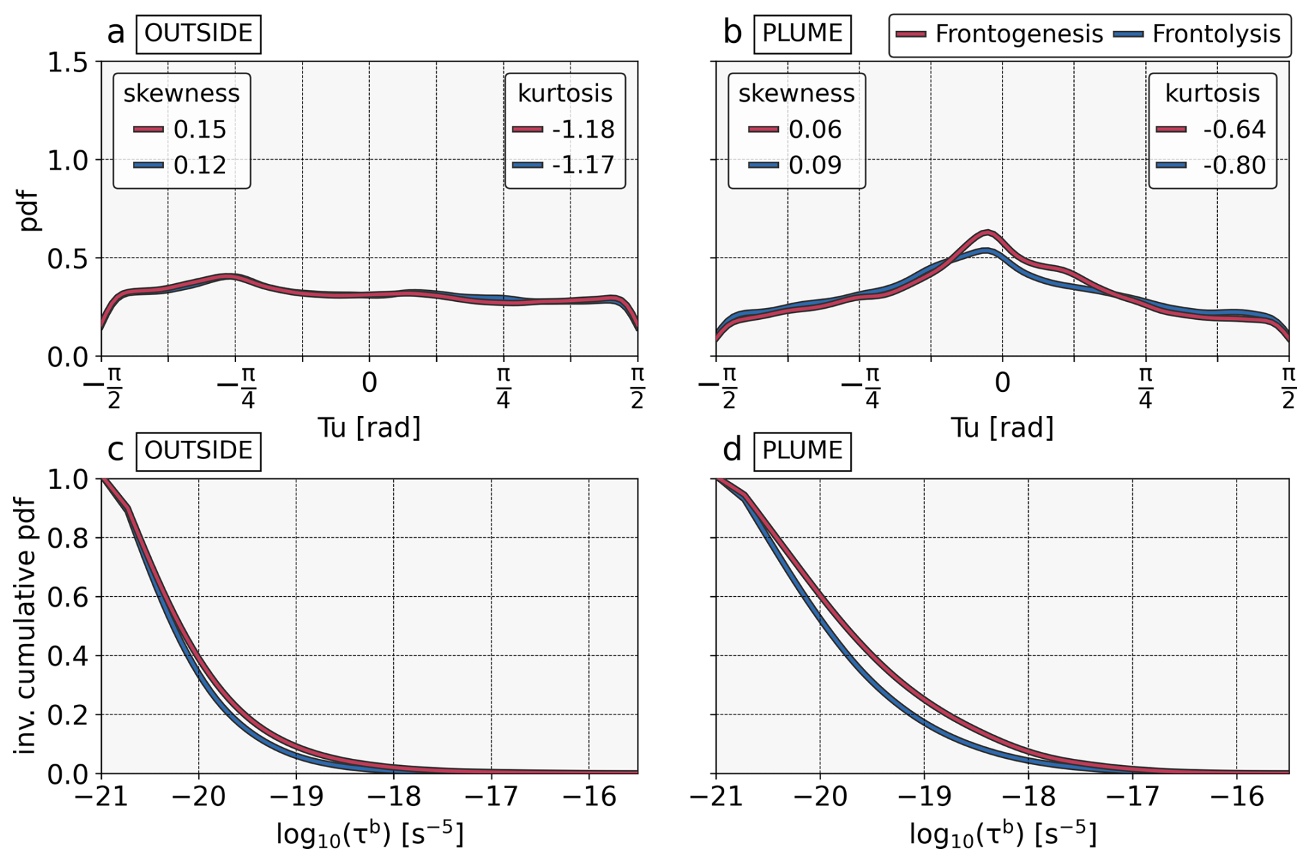
Figure 8 Statistics of modeled Tu and τ^b. (a, b) Pdf of Tu separated between gradients showing frontogenesis (red) and frontolysis (blue), for (a) outside and (b) the plume. (c, d) Inverse cumulative pdf of frontogenesis (red) and frontolysis (blue), for (c) outside and (d) the plume.

Even though the full terms are available from GIGATL1, analyses of τ^b are restricted to the surface. For the sake of completeness, we compared this approximation to the full terms of τ^b, which may, in extreme cases, modulate the fronts' intensity, but does not alter their spatial distribution (see Appendix D). This advocates for the efficiency of the observed strategy in capturing such features by sampling only their horizontal variability. Yet, strong stratification in this tropical region and the presence of the Amazon Plume can scale-up the vertical term and alter the ratio between frontogenesis and frontolysis. The effects of vertical terms are not detailed in this study.

Owing to a simulation capable of representing the magnitude and distribution of buoyancy gradients associated with the Amazon River plume over a wide range of conditions, we now proceed to the spatiotemporal analysis of the simulation to shed light on how the region's dynamics shape T–S relations and fronts on the different plume and outside environments.

5 Spatial distribution of surface fronts

At fine scales, the stirring and straining of tracers by mesoscale and submesoscale motions add to the low-frequency dynamics of the large scales (e.g., Lévy et al., 2018; Fu et al., 2024). In the model, they control the spatial diversity of T–S gradients (Fig. 9a), maintained by the joint action of the Amazon River plume and the NBC (Hellweger and Gordon, 2002). Their interaction gives rise to all T–S relationships, producing different types of gradients (Fig. 9a and b between 56–52° W; 8–10° N; see also Figs. 3 and 7). On 25 March, a retroflecting NBC carrying warm waters rolls up a plume filament. Within the core of the impinging plume filament, the dominance of salinity gradients is striking ($-\frac{\mathit{\pi }}{\mathrm{4}}<\text{Tu}<\frac{\mathit{\pi }}{\mathrm{4}}$; Fig. 9a). East of the plume, the NBC continues to advect freshwater northward, while the swirling motion associated with NBC rings folds gradients into layered structures characterized by alternating dominance of plume salinity and NBC temperature.

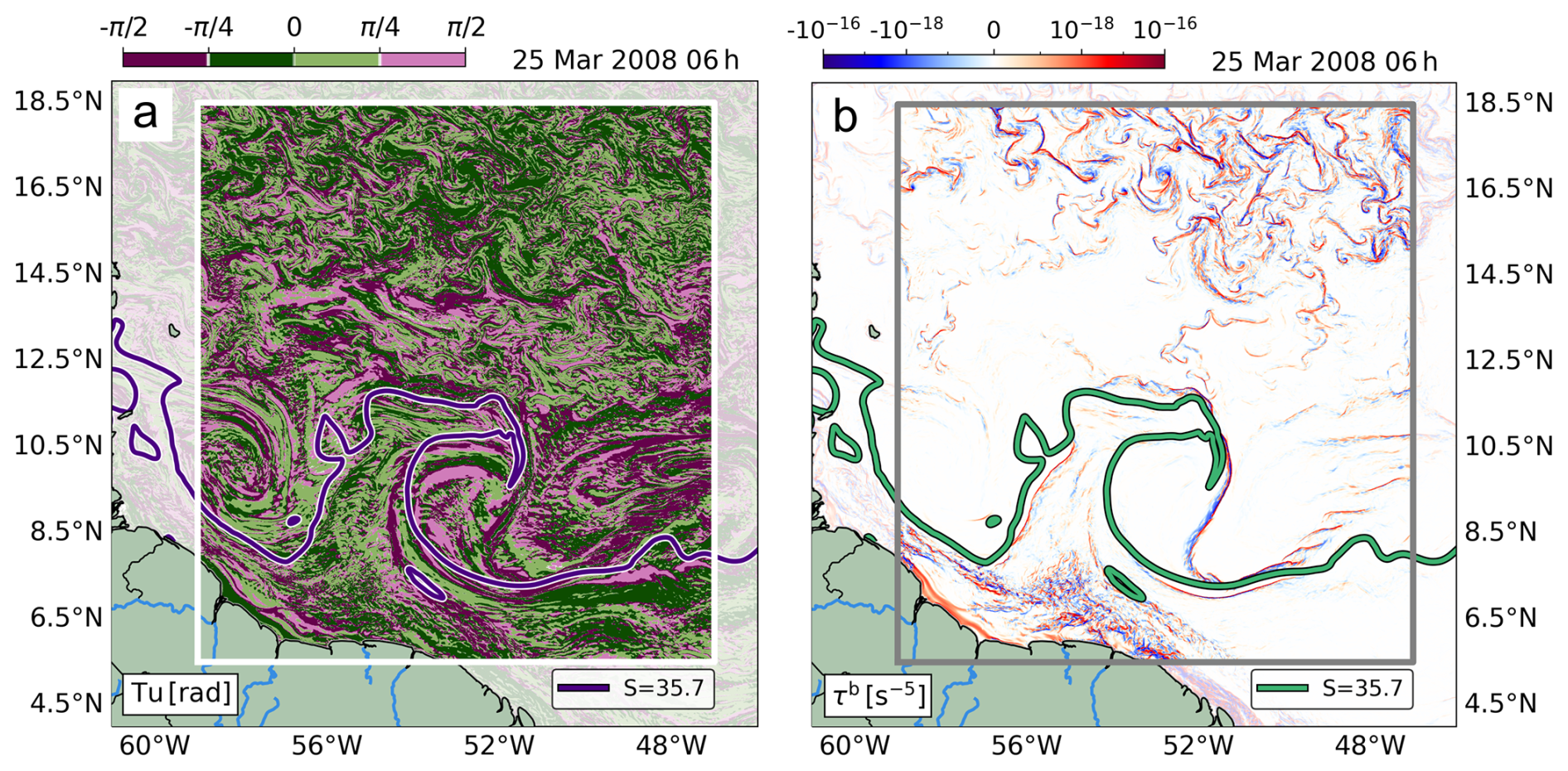
Figure 9 Spatial distribution of (a) the Turner Angle Tu and (b) the Frontogenetic Tendency of Buoyancy τ^b for the snapshot on 25 March 2008, 6 h. The plume region is delimited by the isohaline representing the 0.25 quantile of the salinity probability distribution (dark blue and green lines).

Notably, the scenario shows the formation of an uncompensated front (Tu; Fig. 9a) at the northern edge of the Amazon plume carried offshore by the NBC. Along the retroflecting current, ΔS>0 surpassed by ΔT>0 sets up a temperature-dominated, uncompensated front edge that delimits the NBC–plume interaction region (Fig. 9a). Thus, fronts detaching from the near-shore region are unambiguously related to the NBC retroflection stirring the Amazon Plume. Within the core of the plume, in turn, both compensated and uncompensated fronts are now dominated by salinity. These fronts are still associated with the interaction of the NBC and the Amazon Plume, but occur mostly inside the plume (Fig. 9a).

The frontogenetic tendency of buoyancy (Fig. 9b) display distinct fronts over three domains, with particular dynamics and different geometry:

• i.

  Shelf fronts: broken-up fronts parallel to shore occupy the core of the plume over the continental shelf. Strong τ^b of these fronts follow the coastal flow over the shelf (Candela et al., 1992; Johns et al., 1998) and may be broken-up by processes acting on timescales shorter than the flow advection, such as interaction with normal-to-shore tidal currents (e.g., Candela et al., 1992; Assene et al., 2024) and air–sea interactions (e.g., Spiro-Jaeger and Mahadevan, 2018; Coadou-Chaventon et al., 2024);

• ii.

  NBC-plume interaction fronts: longer arched fronts associated with the NBC interacting with the plume connect the near-shore and oceanic region. They occur either within or at the border of the plume, as similarly shown by Barkan et al. (2019) in the Mississippi plume, and are associated with curved filaments at the border of eddies and meanders (Lapeyre and Klein, 2006; McWilliams et al., 2019); wavelike structures at the plume edge (∼50° W) could be associated with the strong internal tides that interact with the NBC (e.g., Tchilibou et al., 2022, 2025);

a gap in frontal activity separates the plume and western boundary regions from the

• iii.

  Offshore “submesoscale soup”: Away from the direct influence of the NBC (∼15° N), the absence of a strong background strain field allows submesoscale fronts to develop with no preferred orientation, hence the isotropic spatial distribution of what are individually anisotropic (elongated) front structures, characteristic of a submesoscale “soup” away from the influence of the main flows (see e.g., Shcherbina et al., 2013; Barkan et al., 2017a; Srinivasan et al., 2017; Liu et al., 2021). These fronts are instead controlled by the seasonal mixed-layer cycle, intensifying in late winter and spring as shoaling mixed layers become unstable (e.g., Callies et al., 2015; Rocha et al., 2016). A shift in frontal scales occurs from early to late spring (not shown), as larger fronts feed on smaller scales through the inverse energy cascade (e.g., Klein et al., 2008; Dong et al., 2020; Schubert et al., 2020; Naveira-Garabato et al., 2022).

Although not quantified here, submesoscale fronts associated with frontogenesis at 1 km scale also play a role in cascading energy from the submeso scale to smaller scales (Freilich et al., 2023). With a submesoscale resolving simulation, Barkan et al. (2019) showed net frontogenesis associated with river plumes, with ageostrophic convergence near the surface dominating the dynamics of frontal sharpening. In our region, this process will complete (and likely at some point overcome) the classical frontogenesis (Hoskins and Bretherton, 1972) driven by the nondivergent mesoscale stirring due to the NBC.

6 Seasonality of T–S compensation

The spatial distribution of Tu shows large areas dominated by salinity and not restricted to the plume. Temperature-dominated gradients also appear, mostly associated with remarkable flow structures driven by the NBC. Over these structures, a succession of compensated and reinforced density gradients appear to be related to the advection and stirring of freshwater filaments by the NBC (Fig. 9; see also, e.g., Duan et al., 2024). In the northern part of the domain, surface gradients can be dominated by salinity even 1200 km away from the continental shelf. This relatively low salinity may be the result of older strong discharges still present in the region while slowly mixing with local waters (e.g., Muller-Karger et al., 1988; Coles et al., 2013). But how does low SSS reach as far as 20° N? Which processes are involved in the spatio-temporal distribution of gradients and how do they relate to density fronts? A Hovmöller diagram in Fig. 10a illustrates the spatio-temporal evolution (propagation) of surface salinity versus temperature dominance over density gradients. Moreover, a timeseries of pdfs (Fig. 10b) shows the temporal evolution of compensation and reinforcement on density by T–S gradients within the plume.

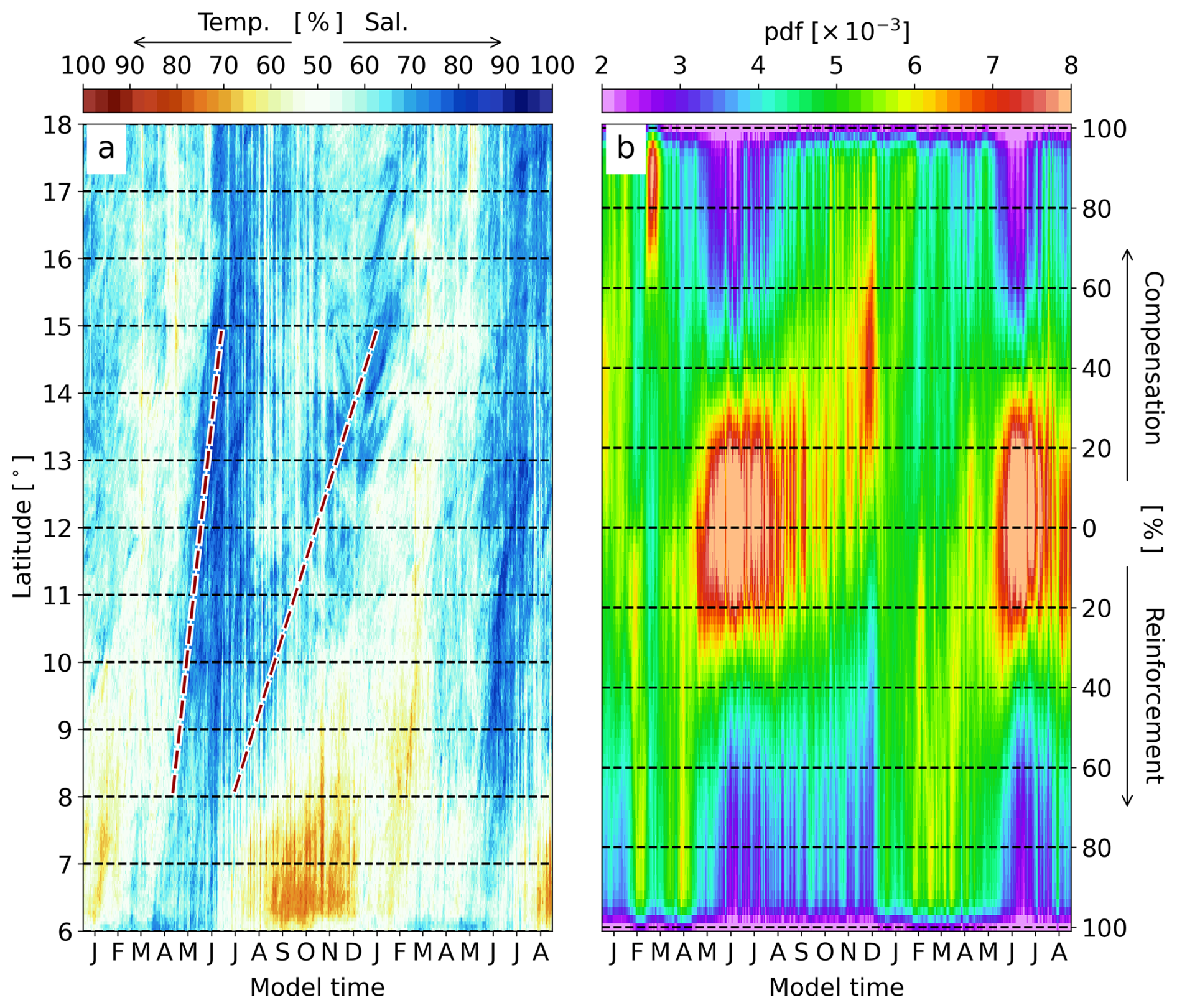
Figure 10 (a) Hovmöller diagram of the percentage of salinity (% Sal.) vs. temperature (% Temp.) dominance in the density ratio during the plume propagation northward (59–47° W; 6–18° N). Model time starts on 1 January 2008. (b) Daily timeseries of the probability density function of the percentage of compensation or reinforcement in the density ratio within the plume region.

To construct Fig. 10, we use Tu to quantify both the T–S relations and their effects on density gradients. First, we calculate the percentage of salinity dominance in surface gradients (i.e., where $\left|\text{Tu}\right|<\mathit{\pi }/\mathrm{4}$), averaged longitudinally between 59–47° W. From 6–18° N, we binned $\left|\text{Tu}\right|$ in 0.05° intervals over 20 months of hourly-averaged snapshots, at 24 h frequency (Fig. 10a). Then, since Tu varies linearly, from the interpretation of Tu, it is possible to define the % of compensation or reinforcement in ℛ by interpolating Tu in each quadrant on a 0 %–100 % scale. For every snapshot, we select points where S<𝒬₂₅ and repeat the computation to obtain daily pdfs.

Between 6–9° N, the prominent seasonality of salinity and temperature dominance reveals a competition between the NBC and the Amazon Plume. In Fig. 10a, % Sal. is highly correlated with the Amazon Plume forcing (r²=0.93; cf. Dai and Trenberth, 2002, not shown) and strongest from April to June. The weak discharge in autumn opens room for the NBC at low latitudes (Fig. 10a). When the NBC is strongest (e.g., Johns et al., 1998), the region between 6–9° N shows the highest % Temp., up to 70 %. The NBC influence rapidly fades offshore, and a north–south, quasi-stationary (∼80 %)% Sal. band appears from April on. Driven by a growing Amazon Plume, a secondary branch of % Sal. begins to expand offshore in late March (Gévaudan et al., 2022), at roughly 11–4 km d⁻¹ (Fig. 10a), consistent with previous drifter observations trapped within NBC rings (e.g., Richardson et al., 1994).

This propagating branch characterizes a “transition zone” (9–15° N) influenced by the advection of salinity gradients by the NBC and its associated mesoscale processes (Reverdin et al., 2021; Gévaudan et al., 2022; Subirade et al., 2023) and mean surface currents that drive the plume toward the north (e.g., Foltz et al., 2015). Strong fronts can be formed by the stirring of salinity gradients by the NBC retroflection and rings. Mesoscale stirring gives rise to gradients that can quickly evolve to submesoscale fronts by an exponential sharpening of those gradients (Gula et al., 2022). Stirring and trapping of the plume by the NBC mesoscale activity could also explain the bifurcation of the % Sal. signal into a direct northward branch and a second branch that breaks off and slowly moves poleward after a virtually stationary period between 9 and 12° N, probably entrained within mesoscale structures (Fig. 10a; e.g., Olivier et al., 2022). Indeed, low SSS anomalies (which drive density gradients in the area) were observed north of the NBC retroflection between June and November (e.g., Ffield, 2005). Low SSS anomalies in this region may be damped by evaporation (e.g., Foltz et al., 2015), although precipitation does not appear to reduce SSS within the plume (Gévaudan et al., 2022).

The northernmost part of the domain (15–18° N) shows the most persistent dominance of salinity on density gradients throughout the year. Away from the NBC and its associated (sub)mesoscale features, low SSS from the quasi-stationary branch is slowly mixed locally. A few months later, the secondary branch of the plume arrives. This high salinity dominance remains in the region until the onset of the “main branch” of the following year, and the number of fronts increases substantially in the transition zone (Fig. 9b). Even with salinity dominance at the surface, the isotropic areas with anisotropic fronts show characteristics of a “submesoscale soup” (e.g., Barkan et al., 2017a; Srinivasan et al., 2017), where fronts are linked to mixed-layer instabilities and the dynamics is fundamentally controlled by the mixed-layer cycle (e.g., Callies et al., 2015).

The ensemble of T–S gradients within the plume exhibits a seasonal cycle in the distribution of compensated and reinforced fronts (Fig. 10b). An expanding plume in spring is still mostly contained northwest along the coast and creates a SSS gradient from the shelf to the open ocean. Assuming salinity βΔS largely dominates over αΔT (Fig. 10a), Tu is virtually zero and, in most density gradients, compensation or reinforcement can decrease or intensify them by only about 20 % (although Fig. 10b does not distinguish salinity or temperature dominance), the rest being essentially driven by salinity (Fig. 10b – months June–August; see also Liu et al., 2026).

In the first half of the year, warmer SST near the shelf presents a negative temperature gradient towards offshore (e.g., Ffield, 2005), which may reinforce density fronts associated with low SSS from the plume (Fig. 10b – months February–May). From June to August, the transport by the NBC and its rings increases and pushes the plume to its maximum extent. In late fall and winter (October–December), a shift in the distribution towards compensation indicates the evolution of gradients within the plume. This is the period when compensation mechanisms through air–sea interaction will be most effective within the plume, for differential surface cooling will act due to a mixed-layer depth-dependent heat loss (e.g., Spiro-Jaeger and Mahadevan, 2018; Coadou-Chaventon et al., 2024). Conversely, a positive heat flux in spring and summer would reinforce the salinity-dominated density gradients to the point where the unbalanced heat uptake leads to dominant temperature gradients on density. However, one must bear in mind that compensation and reinforcing are scale-dependent, so assumptions such as net seasonal heat fluxes involve processes other than mixed layer instabilities and air–sea heat fluxes acting on the mixed-layer depth, SSS, and SST (Spiro-Jaeger and Mahadevan, 2018).

In the Mississippi River plume, Barkan et al. (2017b) showed an overall increase in the tails of Tu pdfs during winter. Moreover, the authors show with a Lagrangian framework that, even if an initial state presents a distribution of Tu centered at zero, a preference for compensated gradients arises over time. This shift occurs gradually during autumn, with a clear predominance of compensated gradients at the beginning of wintertime. We recall that our analysis considers only density gradients with SSS lower than 𝒬₂₅, which can introduce a bias toward reinforced gradients: the mixing of “the old plume” usually creates higher SSS, and evolving fronts in this region can be removed from the analysis.

While air–sea interactions are known to induce compensation to the strongest T–S gradients at small scales in the Amazon Plume (Coadou-Chaventon et al., 2024), facing the gradients galore of the northwestern Tropical Atlantic brings a broader perspective related to the region's peculiar dynamics. Next, we suggest how these dynamics set up some T–S relations observed in the region.

7 Interactions between the Amazon Plume and the NBC

In the previous sections, we showed regions with fronts related to the interaction between the Amazon Plume and the NBC. They are numerous near shore and broken up possibly due to further interactions with high-frequency processes. Offshore, elongated fronts drawn from this near-shore pool align with flow structures. They often come as freshwater filaments advected by the NBC that pierce through a higher salinity background (Fig. 11a) and roll up into a warm-core NBC ring (Fig. 11b; e.g., Ffield, 2005).

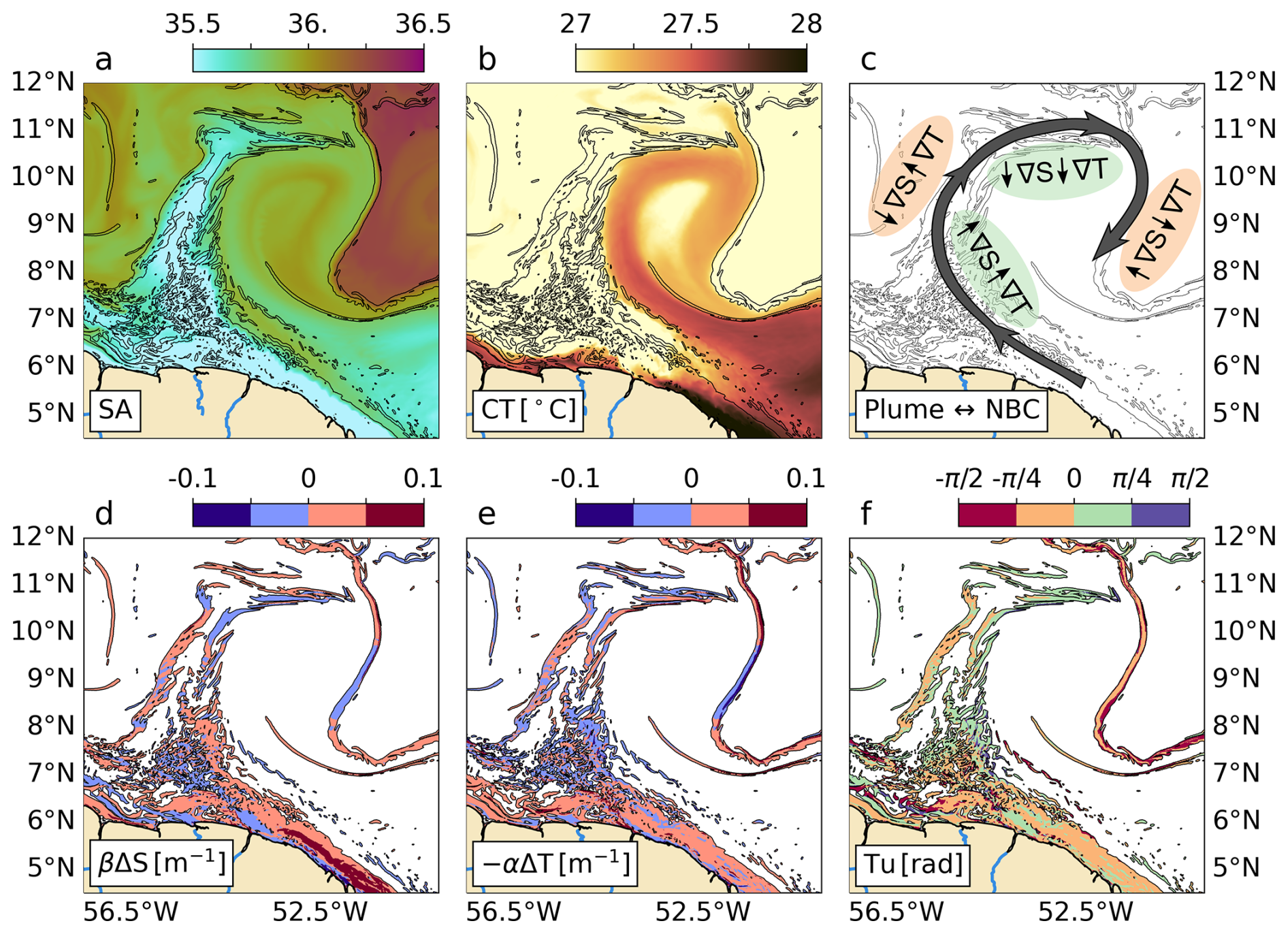
Figure 11 Interaction of the NBC and the Amazon Plume zoomed in from the model on 25 March 2008, 6 h. (a) SA: Absolute salinity; (b) CT: Conservative Temperature; (c) Schematic of compensation (green) and reinforcement (orange) developing on opposite sides of the low-salinity filament; (d) contribution of salinity to density variation; (e) contribution of temperature to density variation; (f) Tu: Turner angle. The blowout of T–S gradients in (d–f) selects areas where $\left|\mathit{\beta }\mathrm{\Delta }S\right|\ge \mathrm{0.01}$ m⁻¹, where thin black contours represent βΔS=0.01 m⁻¹. In (d–f), colors delimit regions of βΔS≥0.01 m⁻¹.

From observations, we suggested that the interaction between the Amazon Plume and the NBC could induce a variety of Tu. Indeed, the resulting front sketched in Fig. 11c shows compensation and reinforcement on opposite sides of the front. This asymmetry arises because the low-salinity filament is embedded in a warmer NBC temperature background. On the warm (inner) side of the filament, the temperature gradient opposes the salinity gradient, producing compensation. On the cooler (outer) side, temperature increases as salinity decreases toward the filament core, so they reinforce each other on the density gradient. The key driver is therefore the sign change in the salinity gradient across the filament, while the temperature gradient remains roughly uniform.

The blowout of T–S gradients in Fig. 11d and e selects areas where $\left|\mathit{\beta }\mathrm{\Delta }S\right|\ge \mathrm{0.01}$ m⁻¹. It further illustrates how salinity and temperature combine to sustain compensation and reinforcement at both sides of the arched filament (Fig. 11f). Crossing the main filament, temperature gradients do not display a clear change in sign due to somewhat uniform west–east gradients. This pattern was briefly reported by Duan et al. (2024) in a cold filament in the Bay of Bengal and appears repeatedly during the formation of NBC rings on our simulation.

If one considers submesoscale fresh filaments developing at the edge of the plume, when considering all T–S gradients this pattern of both compensation and reinforcement shall repeat over a large portion of the domain, yielding the zero-centered distributions of Tu due to the interaction with the plume and the NBC and/or local dynamics offshore. With the region being mainly frontogenetic, the set up of different fronts by the NBC–Amazon Plume interaction (e.g., Figs. 8 and 9) could trigger distinct dynamical responses: while uncompensated fronts are unstable and act on the direct energy cascade and mixing (e.g., Rudnick and Martin, 2002; Srinivasan et al., 2023), the more stable, (partially) compensated fronts can be strained for longer periods, shaping horizontal transport and maintaining their associated vertical fluxes (e.g., Rudnick and Martin, 2002; Zhu et al., 2024). We call for future work to statistically address these mechanisms and their effects on the overall energy budgets of compensated and reinforced fronts.

8 Summary and Conclusions

An expanding Amazon River plume occupied the northwestern Tropical Atlantic during the EUREC4A-OA campaign (as seen in the SSS maps, Reverdin et al., 2021; Coadou-Chaventon et al., 2024). As expected for the transition period from low to high discharge (e.g., Foltz et al., 2015), the plume was relatively well developed, and saildrones sampled both the region outside and the interior of the plume. We observed the sharp increase in the magnitude of density gradients inside the plume, which translates into strong buoyancy gradients at 𝒪 (1–10) km. Unsurprisingly, T–S relations show salinity-dominated density fronts within the plume. Perhaps more interestingly, these fronts display nearly equal contributions of compensation and reinforcement by temperature gradients. Moreover, net frontogenesis is observed both outside and within the plume.

Using a 1 km resolution model, we explored how both the Tu and τ^b observed during EUREC4A-OA are spatially arranged when the Amazon Plume and the NBC interact. The modeled region shows greater variability and extreme fronts in the plume, although the separation between plume and outside is less distinct in the simulation. Three different frontal regimes occur in the domain, one within the plume over the continental shelf, a second associated with stirring of the plume by the NBC, and a third offshore, typical of mixed-layer controlled submesoscale activity. Qualitatively detailing the interaction between the Amazon Plume and the NBC, we show that the mesoscale stirring of the plume by the NBC produces a patchy distribution of Tu, particularly during the formation of NBC rings, where freshwater filaments are rolled up into a NBC temperature background, generating compensated density fronts in the inner portion of the filament and reinforced fronts on the outer rim.

In the northwestern Tropical Atlantic, salinity gradients representative of sharp density gradients dominate the region up to 9° N driven by the seasonality of the Amazon runoff. When the river discharge is weakest and the NBC charges into the region, temperature gradients dominate. Stirring and advection of the plume by the NBC shape the fronts in the transition region from 9–15° N. North of 15° N, the distribution of surface gradients is dominated by salinity all year long, even though in this region their dynamics are most likely to follow the temperature-driven seasonality of submesoscale turbulence (e.g., Callies et al., 2015; Rocha et al., 2016). The distribution of frontogenetic tendency suggests the northwestern Tropical Atlantic as a region of predominant frontogenesis, with both compensated and uncompensated density fronts mostly related to mesoscale low-salinity filaments stirred from the Amazon Plume by the NBC and submesoscale structures developing at the plume edge, with a clear seasonal cycle of compensation and reinforcement linked to the plume size and the NBC strength.

The frontal seascape described here, which is salinity-dominated, seasonally modulated, with coexisting compensated and reinforced fronts, has direct implications beyond physical oceanography. Compensated fronts, being more stable, sustain strong horizontal tracer gradients for longer periods, potentially influencing nutrient supply, phytoplankton patchiness (e.g., Gouveia et al., 2019; Lévy et al., 2018), and ecosystem connectivity (e.g., Giachini-Tosetto et al., 2022). Reinforced fronts, being unstable, drive energetic downwelling that may export surface-enriched Amazon water below the pycnocline on short timescales (e.g., Waite et al., 2016). Distinguishing these two populations of fronts may therefore be essential for understanding the plume's role in regional carbon and nitrogen budgets.

As numerical models continue to improve, they rely on data acquisition at high resolution to tackle current discrepancies and parameterizations for dynamics at small scales. The unprecedented datasets from campaigns such as EUREC4A-OA and other uncrewed vehicles in the global ocean (meet them in a review by Patterson et al., 2025), together with state-of-the-art numerical modeling provide statistical confidence in studying derived quantities at 𝒪(1 km). Our current effort is to explore the dynamics depicted from EUREC4A-OA small-scale observations to help improve the fine-scale ocean modeling of the Amazon Plume outflowing into the Atlantic. Such datasets need to be continuously exploited alongside new observational and modeling efforts to improve our assessment of the Amazon Plume region.

Appendix A: Observed Buoyancy Sharpness variance

In the outside, the ℬ variance gradually increases from ℓ=100 up to 5 km, whereas in the plume the major increase takes place at scales smaller than ℓ=10 km (Fig. A1). The variance of the buoyancy frontal sharpness ℬ is greater in the plume at all observed scales.

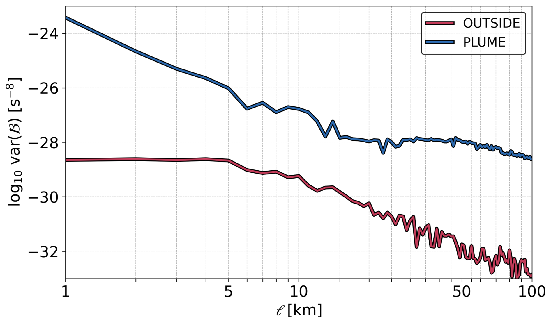
Figure A1 Observed variance of the buoyancy frontal sharpness ℬ in the plume and in the outside.

Appendix B: Plume representation in the model

Appendix B compares the poleward extension of the Amazon Plume of the model with the CATDS CEC SSS satellite product (Boutin et al., 2022) and the ISAS climatology (Kolodziejczyk et al., 2023) in the 59–47° W; 6–19° N region where we conduct our analyses. The satellite data is a regional product for the Amazon region, which combines SMOS and SMAP data with an optimized interpolation scheme that yields a temporal resolution of 2–3 d and ∼50 km effective horizontal resolution. The ISAS17 release is a monthly climatology that combines Argo and Deep-Argo temperature and salinity data with other in-situ measurements between 2002 and 2017 to fill in gaps where Argo sampling is sparse or nonexistent. The ISAS product has 187 vertical levels between 0–5500 m and a ∼50 km horizontal resolution.

We select the 36 isohaline in both model and the available datasets. This isohaline is used in the main text as a reference to identify the Amazon Plume edge in the observations. Then, we took the northernmost latitudinal point for each day (model, satellite), and month (climatology) as shown in Fig. B1.

The model presents a mean SSS comparable to that of the ISAS climatology but slightly overestimates the satellite SSS and underestimates its variability. This is due to a difference in the minimum SSS between the model and the satellite, with strong mixing coefficients leading to a rapid increase in the salinity at the points of river input. Strong mixing may also be related to a “delay” in the poleward displacement of the plume, with an ∼1-month difference between the observed and modeled plume reaching the same latitudes (Fig. B1). The northernmost position of the 36 isohaline in GIGATL1 shows a r²=0.80 (Pearson) linear correlation with the isohaline position depicted by satellite and 0.75 with the one from ISAS. It follows the pattern presented in Gévaudan et al. (2022) for the evolution of the plume area. The latitudinal SSS profile of GIGATL1 is also well correlated with observations over time (0.87 for both satellite and ISAS). Therefore, even if not at the exact same period, our simulation can reproduce the SSS seasonal cycle as well as the strength of buoyancy gradients, which gave us confidence in carrying out the analyses in this study. We will address the noted discrepancies in future versions of the simulation.

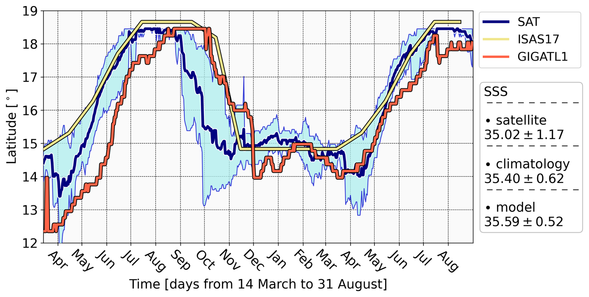
Figure B1 Northernmost position of the 36 isohaline between 14 March and 31 August from satellite (dark blue line mean with 80 % of the distribution in light blue), climatology (light yellow line), and model (red line). For the satellite data, five 18-month series (light grey lines) span data from 2016 to 2021. The monthly climatology is reorganized to display 18 months of data. The model years (March 2008–August 2009) are referenced due to the data used for forcing. Product keys: SAT – satellite product is a regional product distributed by CATDS CEC (Boutin et al., 2022), providing a combination of SMOS and SMAP sea surface salinity data; ISAS17 – stable (delayed time) Argo climatology distributed by Argo France (Kolodziejczyk et al., 2023); GIGATL1 – CROCO numerical simulation (Gula et al., 2021).

Appendix B acknowledgments: We thank G. Reverdin and J. Boutin for the discussion of SSS products and for the CEC CATDS High Resolution V0 Sea Surface Salinity maps, produced by LOCEAN/IPSL (UMR CNRS/UPMC/IRD/MNHN) laboratory and ACRI-st company that participate to the Ocean Salinity Expertise Center (CECOS) of Centre Aval de Traitement des Données SMOS (CATDS). This product (Boutin et al., 2022) is distributed by the Ocean Salinity Expertise Center (CECOS) of the CNES-IFREMER CATDS, Plouzane (France). ISAS temperature and salinity monthly gridded field products (Kolodziejczyk et al., 2023) are made freely available by SNO Argo France at LOPS Laboratory (supported by UBO/CNRS/Ifremer/IRD) and IUEM Observatory (OSU IUEM/CNRS/INSU) at https://doi.org/10.17882/52367.

Appendix C: Adaptive definition of the plume in the simulation

To ensure numerical consistency and reduce the effect of numerics on variables at grid scales, gradients are smoothed in the model compared to the observed gradients at the same scales. This hinders the ability of the model to capture the abrupt changes marking the transition from the plume region to the outside.

In Fig. C1, we display the SSS gradient at the model grid scale. Those gradients, smoothed by a 50 km rolling mean in both x and y directions, visually mark the separation from the plume and the outside regions. Here, we show contours of the 20 %-strongest mesoscale SSS gradients, which roughly coincide with the isohaline representing 25 % of the salinity probability distribution for each snapshot. This yields S=35.7 for the 25 March 2008, 6 h snapshot discussed in the study. We also apply this 25 % threshold to retrieve the plume from snapshots daily and thus compute the percentage of density compensation and reinforcement (main text Fig. 8b).

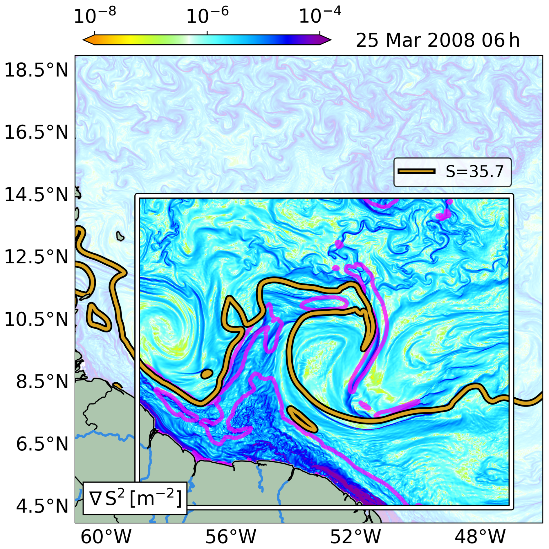
Figure C1 Model surface salinity gradient on 25 March 2008, 6 h. The plume region is delimited by the isohaline representing the 0.25 quantile of the salinity probability distribution (golden line). Purple lines represent the 20 % strongest mesoscale SSS gradient.

Appendix D: Advective Frontogenetic Tendency terms

We briefly evaluate the role of the vertical terms in the advective frontogenetic tendency of buoyancy equations by subtracting τ^b calculated from horizontal terms alone from the total τ^b in Fig. D1.

Comparing snapshots from the simulation, the vertical terms modulate the magnitude of gradients, but the relative strongest differences [𝒪(10⁻¹⁸) s⁻⁵] are 2 orders of magnitude smaller than the strongest gradients [𝒪(10⁻¹⁶) s⁻⁵] and representing 0.1 % (Fig. D1, right panels). Moreover, the spatial distribution of the gradients is unaltered, confirming that fronts are set up mainly by horizontal processes (Barkan et al., 2019) and vertical processes either intensify or reduce their magnitude.

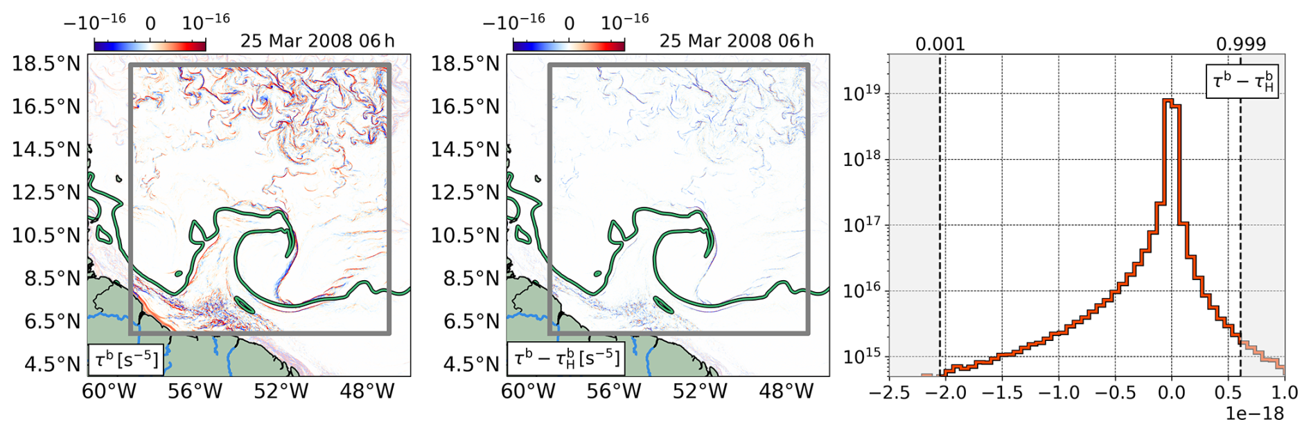
Figure D1 Comparison between full and horizontal terms of the advective frontogenetic tendency for buoyancy. The green line represents the isohaline 35.7, i.e. the 25 % quantile of the surface salinity distribution. The gray box set the limits [59–47° W; 6–181.5° N] where the analysis was conducted. (From left to right) τ^b with full terms from (4); difference between full and horizontal (5) τ^b; and the pdf of τ^b–${\mathit{\tau }}_{\mathrm{H}}^{\mathrm{b}}$.