North Atlantic response to a quasi-realistic Greenland meltwater forcing in eddy-rich EC-Earth3P-VHR hosing simulations

The vast majority of studies examining the impact of freshwater from ice sheet melting on the Atlantic Meridional Overturning Circulation (AMOC) use climate models that cannot resolve mesoscale ocean processes and do not include an accurate spatio-temporal distribution of the freshwater forcing. These two factors critically affect the nature of the AMOC response. Our study partially fills that gap with a set of three hosing experiments using perpetual 1950 radiative forcing with the global configuration of the eddy-rich EC-Earth3P-VHR climate model. The model is forced for 21 years with a spatial and monthly distribution of Greenland meltwater fluxes derived from a product based on observations and model simulations. An annual average close to 0.04 Sv is released on top of the simulated model river runoff, which is vertically distributed in the coastal points connected to each hydrological basin.

Within the first year, we observe a response of reduced salinity in the Greenland and Labrador currents. Since the beginning of the experiments, these boundary currents also experience an acceleration and cooling. The cooling arises because freshwater-induced stratification suppresses vertical mixing, reducing the entrainment of warmer subsurface waters into the surface layer of the boundary currents. The meltwater fluxes also lead to a rapid weakening of the AMOC at subpolar latitudes due to circulation adjustments forced by the changes in density gradients, with the salinity-driven density reduction outweighing the temperature-driven density increase. Around year 7, deep mixing in the Labrador Sea begins to weaken as freshwater anomalies accumulate through lateral exchanges with the boundary currents. This weakening in deep mixing affects the Deep Western Boundary Current (DWBC), which warms up at the OSNAP section, and sequentially further weakens the AMOC, resulting in an even stronger reduction that reaches also the subtropical latitudes. After the 21 simulated years, the AMOC has weakened by almost 3 Sv at 60.2° N in density space, which represents a ∼20 % reduction of the climatological value in the control, 14.9 Sv. In the context of the North Atlantic, a basin-wide decrease of 1.3 Sv is measured between 10–65° N, which represents about 10 % reduction of the control reference, 13 Sv. This AMOC reduction is strong enough for some global climate impacts to emerge, such as a “bipolar seesaw” temperature response.

1 Introduction

Anthropogenic global warming is forcing the Greenland Ice Sheet to melt, injecting a large amount of freshwater into the surrounding ocean (Bamber et al., 2018; Pattyn et al., 2018). The increased freshwater is expected to reduce surface density, enhancing vertical stratification in the Subpolar North Atlantic (SPNA), thereby inhibiting deep mixing (Böning et al., 2016). This reduces the deep water formation, which is linked to the weakening in the Atlantic Meridional Overturning Circulation (AMOC) (Jackson and Wood, 2018; Martin et al., 2022; Bellomo et al., 2023; Jackson et al., 2023; Martin and Biastoch, 2023; Ma et al., 2024; Wei and Zhang, 2024).

Previous studies with different climate models have highlighted important global climate impacts following a collapse or substantial weakening of the AMOC, characterized by widespread changes in surface temperature and precipitation. By reducing the northward heat transport, AMOC reductions induce a “bipolar seesaw” temperature response, with pronounced cooling across the Northern Hemisphere (NH) balanced by modest warming in the Southern Hemisphere (SH) (Jackson et al., 2015; Liu et al., 2020; van Westen et al., 2024; Diamond et al., 2025). This anomalous interhemispheric temperature gradient drives a southward displacement of the Intertropical Convergence Zone (ITCZ) (Jackson et al., 2015; Liu et al., 2020; Orihuela-Pinto et al., 2022; Bellomo et al., 2023; Ma et al., 2024), a reduction in precipitation over NH mid-latitudes (Jackson et al., 2015; Bellomo et al., 2023) and a strengthening of the Pacific Walker circulation (Orihuela-Pinto et al., 2022). The associated changes in atmospheric dynamics can lead to complex regional impacts: experiments with a 60 % reduction of the AMOC in eddy-parameterised climate models show that while the intensified wintertime NH jet stream reduces the frequency of prolonged cold spells over much of Europe (Meccia et al., 2023), the summer weakening of the jet stream increases the frequency of Ural atmospheric blocking, contributing to more frequent heatwaves in Eastern Europe (Meccia et al., 2025). In polar regions, reduced northward heat transport leads to a slowdown in Arctic sea ice loss (Liu et al., 2020), while concurrent increased southward ocean heat transport in the Southern Ocean causes multidecadal local surface warming and sea-ice loss (Diamond et al., 2025). Crucially, AMOC weakening also diminishes the ocean's ability to transport carbon-rich waters to the deep ocean, thereby reducing ocean carbon uptake (Schaumann and Alastrué de Asenjo, 2025).

Freshwater hosing experiments aim to isolate the impact of ice sheet melted waters on the climate system using model experiments (Devilliers et al., 2021; Martin et al., 2022; Swingedouw et al., 2022; Bellomo et al., 2023; Jackson et al., 2023; Martin and Biastoch, 2023; Meccia et al., 2023; Schiller-Weiss et al., 2023; Devilliers et al., 2024; Ma et al., 2024; Oltmanns et al., 2024; Schiller-Weiss et al., 2024; Wei and Zhang, 2024; Diamond et al., 2025; Meccia et al., 2025). These experiments have also become a popular technique for studying the potential recovery of the AMOC after a strong weakening. In particular, the North Atlantic Hosing Model Intercomparison Project (NAHosMIP) aims to study the stability of the AMOC using coupled climate models with resolutions ranging from eddy-parameterised (approximately 100 km of horizontal resolution) to eddy-permitting (approximately 25 km of horizontal resolution) (Jackson et al., 2023). NAHosMIP proposes two different protocols for injecting freshwaters into the North Atlantic: a uniform widespread injection from 50° N to the Bering Strait and a more realistic injection localized around Greenland with an exponential decay up to 300 km from the coast. Their main objective is to study AMOC recovery in Coupled Model Intercomparison Project phase 6 (CMIP6) models by shutting down the forcing after a set number of years (e.g. 50 years of hosing and 100 years of recovery). From a total of eight models, half recovers from a weak AMOC state, while the other half remains in the weak state. They also conclude that these differences in behaviour can not be explained by model resolution (within the resolutions considered) or mean climate state. However, NAHosMIP does not include eddy-rich simulations, which may have a different response due to the impact of mesoscale eddies and properly resolved boundary currents.

Resolving mesoscale ocean eddies reduce biases in the mean state of the ocean, particularly with regard to salinity in the SPNA (Jüling et al., 2021; Frigola et al., 2025). Mesoscale eddies and better resolved boundary currents also improve AMOC pathways and its variability (Hirschi et al., 2020). Therefore, eddy-rich models are ideal to conduct a more in depth investigation of how a realistic meltwater forcing would affect the AMOC and its impacts in the coming years. Few studies have already shown the impact of resolving eddies in the distribution of freshwater in the SPNA (Böning et al., 2016; Martin and Biastoch, 2023).

Exploring long-term responses is challenging due to the significant computational needs to run climate-scale simulations, and the need to consider ensembles to disentangle the forced signals from those of internal origin. The vast data volumes generated by eddy-rich models is another important constraint. Therefore, to make the most of the finer resolution, a protocol with a greater focus on the imminent transient response than on long-term equilibrium is needed. An overly idealised Greenland hosing configuration, e.g. applying a uniform freshwater flux across the North Atlantic rather than distributing it according to the observed drainage basins and seasonal cycle results in an unrealistic spatial distribution of the injected freshwater and potentially bias the modelled ocean response (Goldsworth, 2026). A potential way forward is the new community protocol presented in Schmidt et al. (2025), which provides observation-based datasets of absolute and anomalous freshwater fluxes from the Greenland and Antarctic ice sheets, broken down by drainage basin and freshwater pathway (runoff, subglacial discharge, and solid ice discharge), intended for implementation in models without interactive ice sheets. So far, only a few studies have combined a realistic spatial distribution and seasonality of the meltwaters with eddy-rich simulations (Martin and Biastoch, 2023; Schiller-Weiss et al., 2023, 2024), and these are limited to eddy-rich resolution only in the North Atlantic rather than globally.

This paper presents a set of Greenland freshwater hosing experiments conducted with EC-Earth3P-VHR, an eddy-rich model developed for the High-Resolution Model Intercomparison Project (HighResMIP; Haarsma et al., 2016). To our knowledge, this is the first time a coupled global climate model with an eddy-rich ocean and a high resolution atmosphere has been used with such a realistic temporal and spatial distribution of meltwater fluxes around Greenland. Section 2 describes the methods, including the model configuration and experimental setup (Sect. 2.1) and significance tests considered in the analyses (Sect. 2.2). Section 3 describes the results and includes Sect. 3.1 that explores the response of the AMOC to the freshwater hosing, Sect. 3.2 that characterises the wider ocean changes across the North Atlantic, Sect. 3.3 that explores water mass transformation (WMT) in the SPNA, Sect. 3.4 that investigates how these responses evolve over time and relate to one another, and Sect. 3.5 that examines the atmospheric impacts at the global scale. Section 4 summarizes the conclusions and discusses the remaining open questions.

2 Methodology

2.1 Experimental set-up

We use the global coupled climate model EC-Earth3P-VHR (Moreno-Chamarro et al., 2025), an eddy-rich version of the model specifically developed within the PRIMAVERA project to contribute to the first phase of HighResMIP (Haarsma et al., 2016), as part of the CMIP6 initiative. This model version uses the atmospheric IFS cy36r4 model, the ocean NEMO model in its version 3.6, and the sea ice LIM3 model. This eddy-rich configuration of the model has an approximate grid spacing of about 8 km in the ocean (ORCA12 grid) and about 16 km in the atmosphere (T1279 grid), both at mid-latitudes.

We leverage the high-resolution of the model to propose a quasi-realistic approach to freshwater hosing. This includes realistic spatial and seasonal distributions, as well as an idealised magnitude that is stronger than the expected discharge under current global warming scenarios. The larger amplitude is intended to increase the signal-to-noise ratio in the response. We apply the freshwater hosing according to a spatial and monthly distribution derived from Bamber et al. (2018), which is based on observations and high-resolution regional model runs (see Fig. 1). We inject a freshwater flux during the melting months (May–September, according to Bamber et al., 2018), which peaks in July (see Fig. 1a). The average flux over these five months is 0.1 Sv ($\mathrm{1}\mathrm{Sv}={\mathrm{10}}^{\mathrm{6}}{\mathrm{m}}^{\mathrm{3}}{\mathrm{s}}^{-\mathrm{1}}$), equivalent to an annual average of 0.0419 Sv or a total of 1322 km³ yr⁻¹. This quantity is slightly smaller than the idealized 0.05 Sv on annual average used in other similar studies (Martin et al., 2022; Martin and Biastoch, 2023; Wei and Zhang, 2024). The imposed flux is almost 4 times the recent observational estimates: The IMBIE Team (2020) gives a peak of $\mathrm{345}\pm \mathrm{66}{\mathrm{Gtyr}}^{-\mathrm{1}}$ of Greenland ice lost in 2011, equivalent to 0.011±0.002 Sv. Taking into account the climatological river runoff and iceberg calving fluxes in the control simulation (0.0047±0.0016 Sv and 0.0205±0.0060 Sv respectively, computed over 53 years), the total annual average freshwater injection around Greenland in the hosing experiments increases up to 0.0671±0.0062 Sv (i.e., $\mathrm{2120}\pm \mathrm{200}{\mathrm{km}}^{\mathrm{3}}{\mathrm{yr}}^{-\mathrm{1}}$; see Fig. B1a in Appendix B for associated monthly climatologies). This amount is about 2.3 times the estimations for the total freshwater flux from Bamber et al. (2018) for the 1962–1995 period and about 1.5 times the most recent estimates for the 2010–2016 period.

We include the freshwater as an additional term to model river runoff (Fig. B1 shows the extra runoff input to the model) that is evenly and instantaneously distributed along several ocean coastal points connected to each hydrological basin in the vicinity of the major river outlets, at 0 psu and local seawater temperature. The runoff is uniformly distributed throughout the upper ocean until a given depth in order to avoid numerical and physical problems (Gurvan et al., 2017). The depth of the distribution depends on the water discharge of the basin; the larger the basin discharge, the deeper the distribution. More specifically, around Greenland, most of the water is added to the surface within the upper 0.94 m, with an average depth at which runoff is injected of 1.78 m, reaching 243.76 m at some coastal points. This implementation uses the river runoff routine available in the CMIP6 EC-Earth model (more details in Döscher et al., 2022). However, we use an improved version of the runoff mapper, in which Greenland is partitioned into six sub-drainage basins corresponding to its main glaciological drainage basins (see Fig. B1b), instead of the single Greenland-wide drainage basin in the original implementation. We do not apply compensation for the salinity, as this does not happen in the real world; therefore, the global mean salinity is not conserved.

We run three ensemble members of 21 years, branching off from three different initial states of the HighResMIP 1950-control Moreno-Chamarro et al. (2025) representing a weak, a moderate and a strong AMOC states, corresponding to 11.4, 12.5, and 14.5 Sv respectively at 45° N, compared to the average value of 12.8 Sv in the full control. The start dates are additionally chosen to minimise overlap between experiments, ensuring there was at least a 15 year gap between them. To avoid the effects of a strong initial model drift, derived from the HighResMIP spin-up of 50 years, the first 30 years of the control are also discarded when selecting the start dates. The control uses perpetual radiative forcing conditions from 1950 and will be used as the benchmark experiment (control) to isolate the effects of the hosing. The three hosing runs use the same freshwater flux and constant 1950-forcing. Martin-Martinez et al. (2025) gives a detailed analysis of the mean state and internal variability of the SPNA and AMOC in the control experiment Moreno-Chamarro et al. (2025) provides a broad documentation of its mean state and biases and compares them with those in two lower resolution counterparts, and Frigola et al. (2025) describes its key mean state and biases in the North Atlantic in the context of other other eddy-rich and eddy-parameterised models using historical simulations. The volume overturning streamfunction has been computed as described in Martin-Martinez et al. (2025), while the WMT analysis has been done following Petit et al. (2023) but using wfo model output variable for freshwater fluxes, which combines all the model's freshwater fluxes into the ocean, including the forced Greenland freshwater.

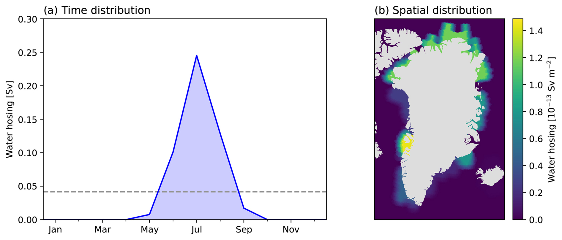
Figure 1 (a) Total monthly freshwater forcing time distribution and (b) May–September averaged freshwater forcing runoff spatial distribution. Values computed from the averaged difference in the runoff (model output) for the first year of each hosing member. The dashed line in (a) indicates the annual average of the forcing. This figure corresponds to the smoothed and interpolated input data, shown in Fig. B1, after being smoothed by the model coupler.

2.2 Results evaluation

The anomalies between the hosing and control experiments are computed by matching the years between both experiments after the initialisation, i.e., the hosing member initialised in 1987 is matched with its respective 21 year period in the control (1987–2007) year-by-year, and the same is done for the other members with their respective control years. This is intended to account for any residual model drift (see Fig. 3 from Moreno-Chamarro et al., 2025) and align the phase of internal climate variability. Although the atmosphere could evolve into different states of internal variability, the low-frequency variability is likely to be preserved due to the relatively short length of the simulations. The statistical tests are tailored to the relatively small ensemble size, with only three members.

Statistical significance of time-mean anomalies is assessed using a bootstrap method. For each grid point, the sample consists of annual anomalies (or seasonal/monthly for variables computed in specific seasons/months such as sea ice or mixed layer depth) pooled across all three ensemble members, which provides three times the number of averaged years. For example, the average of surface salinity anomalies in Fig. 4a is based on a sample of 30 elements (10 annual anomalies × 3 members). We then generate 1000 bootstrap replicates by resampling this pooled sample with replacement and computing the mean of each replicate. Finally, we compute the 95th percentile of the 1000 bootstrap means to determine whether the difference is significant at the 95 % confidence level.

In time series and Hovmöller diagrams, bootstrap cannot be applied with the same method, as we would only be able to use the three elements as the original sample. Therefore, we simply check if the anomaly sign is consistent across the three members. However, as alignment between the three members may frequently occur by chance, we assume here that three consecutive years of coherent, physically explainable signal is sufficient to distinguish a forcing-induced response from a spurious alignment due to internal variability.

All the scientific analyses are performed using well-established open-source scientific programming languages and tools. Most of the analyses are performed directly with Python and ESMValTool v2.12.0 (Righi et al., 2020; Andela et al., 2025a, b), a software package specifically created to facilitate a rigorous evaluation of CMIP simulation outputs that is especially useful to compare multiple models with observational datasets.

3 Results

3.1 Meltwater impacts on the AMOC

We first examine the volume overturning streamfunction to determine how and when the freshwater hosing impacts the AMOC. Figure 2a shows the time evolution of the maximum overturning in depth space at 33.8° N, which is the latitude where the AMOC exhibits the strongest response to the forcing over the last 10 years (Fig. 3a), that is, when the magnitude of the decadal anomaly is maximum. We note that while this choice helps for illustrative purposes, the selected latitude may not necessarily represent a basin-wide response. This AMOC index shows no sign coherent slowdown during the first 7–10 years, when both ensemble means show differences that are consistent with internal variability. After that, it starts weakening over time in response to the additional meltwater, with the maximum weakening happening during the last 5 years.

The maximum change in the AMOC in density space happens at higher latitudes, 60.2° N. The AMOC anomaly at that point starts being sign coherent in year 5, much earlier than the signal at 33.8° N in depth latitudes for which it happens in year 12. To contextualise the different response timings depending on the vertical coordinate, we note that the overturning streamfunction in density space tracks buoyancy-driven changes in water mass properties (e.g. in Labrador Sea Waters; LSW) more directly than in depth space, for which the signal is smeared by the projection onto fixed depth levels (Foukal and Chafik, 2024). As a result, the hosing signal in density space deviates from the control from the beginning of the simulation ensemble, and when normalised by the temporal standard deviation of the control, the signal-to-noise ratio is 1–3 times higher than at 33.8° N in depth space (Fig. B2), indicating that density coordinates provide a clearer separation between the forced response and internal variability. We can indeed expect the signal to develop faster in density space, as the maximum is located at higher latitudes, closer to the place where the freshwater is injected. The AMOC in density space also shows a more robust response because it shows weaker oscillations due to internal variability, as evidenced in the corresponding ensemble spread.

The delayed response in depth space at 33.8° N indicates that the freshwater injection needs some years to significantly impact the lower latitudes. Thus far, comparisons have focused on contrasting responses in two different coordinates and latitudes, which provides an incomplete picture of the large-scale response. From now on, we will focus most of our analysis on the last 10 years of the hosing simulation, to remove the initial years where the signal of the forcing in the AMOC is too small compared to the noise from internal variability. This approach will also allow us to compare depth and density spaces consistently across latitudes.

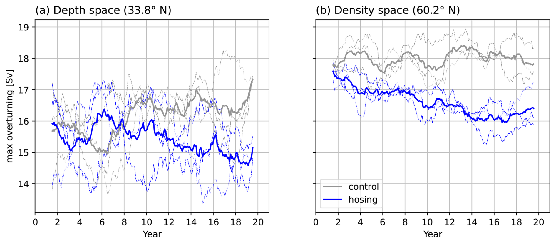
Figure 2 Monthly volume overturning streamfunction in (a) depth space at 33.8° N and (b) potential density space at 60.2° N in the Atlantic basin. The solid lines are the ensemble averages, each member and its corresponding control year are plotted with a unique linestyle. The values have been computed with monthly averages and filtered with a 36 month (3 year) moving average. The latitudes were selected where the corresponding maximum change in the last 10 years happens, see Fig. 3.

The difference in volume overturning streamfunction in depth space for the last 10 years between the control and freshwater hosing experiments shows a significant weakening in the AMOC across all latitudes (Fig. 3a). The hosing signal is strongest at around 1000 m and 33.8° N, where the AMOC weakens by 1.4 Sv on decadal average, equivalent to a 8.6 % of the 16.5 Sv control climatological value. The latitudinal band from 40–50° N exhibits an important reduction that exceeds 1 Sv and is the region with the highest difference relative to its mean reference value. By contrast, the subtropical region (10–20° N) exhibits a more moderate weakening in the order of 0.5 Sv. Overall, the average reduction between 500–1000 m and 10–65° N is about 0.7 Sv, representing a 6.5 % reduction with respect to the equivalent 11.6 Sv control average value. This shows that 21 years of hosing with an annual average freshwater anomaly of ∼0.04 Sv is sufficient to produce a detectable weakening in the AMOC, although this remains far from representing a full AMOC collapse. This response is weaker than in the study of Swingedouw et al. (2022), who report a weakening of about 2 Sv after 13 years of a comparable freshwater forcing (∼0.035 Sv anomaly). Studies applying substantially larger forcings, such as Jackson et al. (2023) with 0.1 Sv, or operating on centennial timescales with time-varying freshwater inputs (van Westen et al., 2024), are less directly comparable given the differences in experimental design, but collectively support the notion that the magnitude of the AMOC scales with the intensity and duration of the freshwater perturbation.

The AMOC in density space shows again a stronger and more coherent response across latitudes than in depth space (Fig. 3b). Indeed, the entire 35–62° N band experiences a reduction above 2 Sv, almost twice as big as for the AMOC in depth space. The maximum reduction is located at 60.2° N, where it reaches 3.0 Sv, a 19.9 % of the control climatological benchmark (14.9 Sv). Overall, the decrease between 1027.4–1027.6 kg m⁻³ and 10–65° N is about 1.3 Sv, equivalent to a 10.0 % of the control reference (13.0 Sv). The maximum impact consistently happens from 65–10° N for the same density level. This is expected, given that water flows along isopycnals and not isobaths (Foukal and Chafik, 2024).

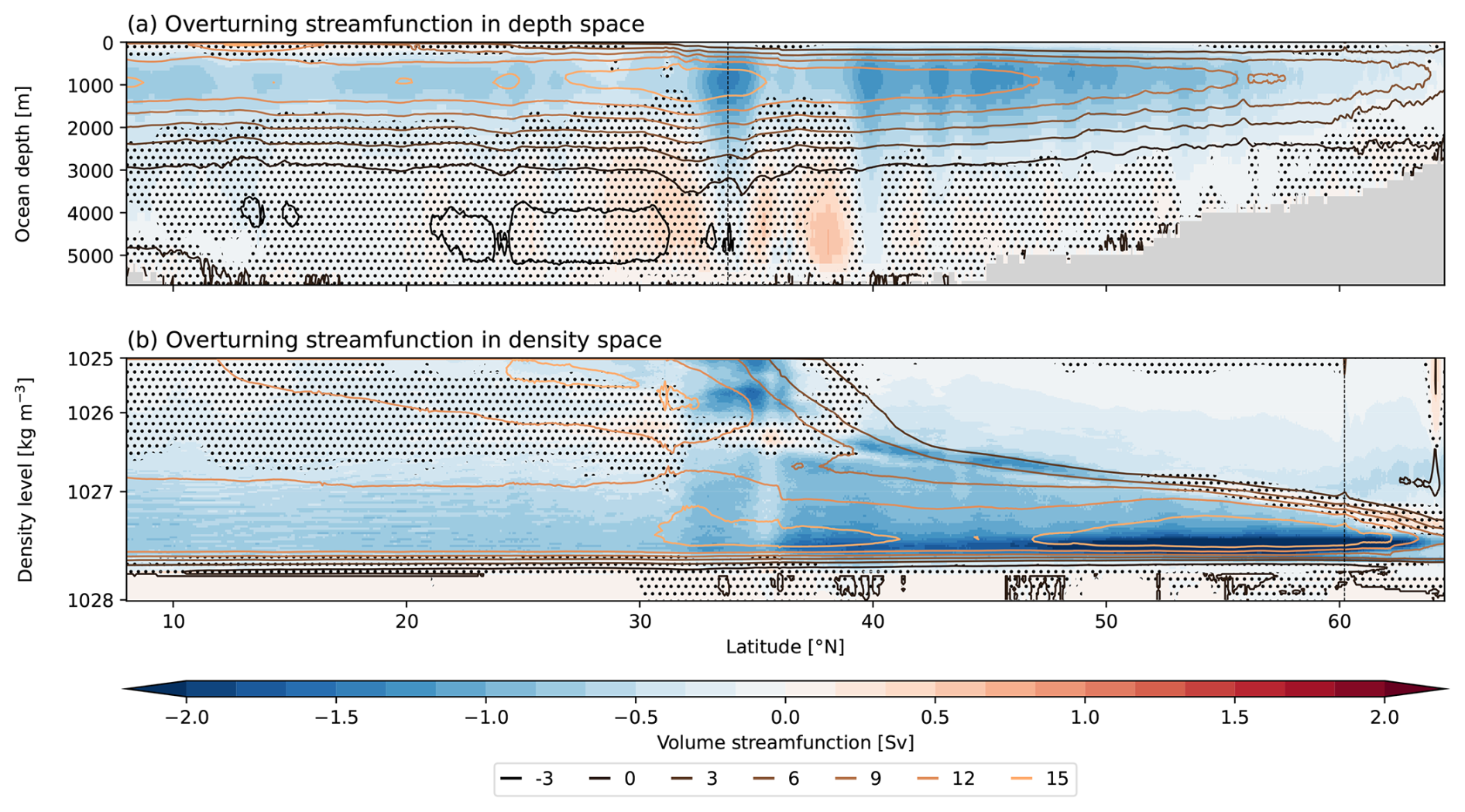
Figure 3 Response to the hosing in the last 10 simulated years (i.e. years 12–21 after the hosing is started) for the overturning streamfunction in (a) depth space and (b) density space; filled coloured contours represent the ensemble-mean anomalies of the hosing with respect to the reference control and the contour lines the climatology of the control. Non-significant values as identified by the bootstrap methodology are masked with dots to improve the visibility over the significant areas. Vertical dashed lines mark the latitude where the maximum difference happens; 33.78° N in depth space and 60.21° N in density space.

In the next Section, we investigate buoyancy changes in the main deep convection areas of the North Atlantic to understand their potential impact on the LSW and, subsequently, on the AMOC. For that, we examine how different thermodynamic variables have changed in the Subpolar North Atlantic (SPNA) in the last 10 years of the simulations.

3.2 Changes in the subpolar region

As expected, the most direct impact of the meltwater forcing on the SPNA is in the salinity field. Figure 4a shows the sea surface salinity (SSS) anomalies in the last 10 years, which exhibit significant negative values over the whole SPNA area. The largest changes due to the injected freshwater – with SSS losses exceeding 0.4 psu – occur around the Greenland coast and continue along the main boundary currents. Some freshening anomalies are found to penetrate into the Labrador Sea interior, where the average reduction in SSS is close to 0.1 psu. The differences in intensity and significance between the anomalies in the Nordic-Irminger seas and Labrador Sea suggest that the boundary-interior exchange is more important in the Labrador Sea, which is consistent with previous studies showing that the boundary-interior exchanges are more important in the West Greenland Current due to local effects of meanders and eddies (Georgiou et al., 2020; Pacini and Pickart, 2022; Swingedouw et al., 2022; Duyck and De Jong, 2023; Spall et al., 2024). This also suggests that the Labrador Sea may play an important role in the AMOC response. Some of the freshwater anomalies coming out from the Labrador Current appear to reach the North Atlantic Current (NAC), where surface water salinity decreases by more than 0.1 psu. Significant surface freshening anomalies extend southward to the position of the Gulf Stream in the west (approx. 40° N) and to 35° N in the center and east Atlantic. There is a small imprint in lower latitudes of positive salinity anomalies, likely related to the slowdown in the AMOC and the associated reduction in the northward salinity transport (Fig. B5a).

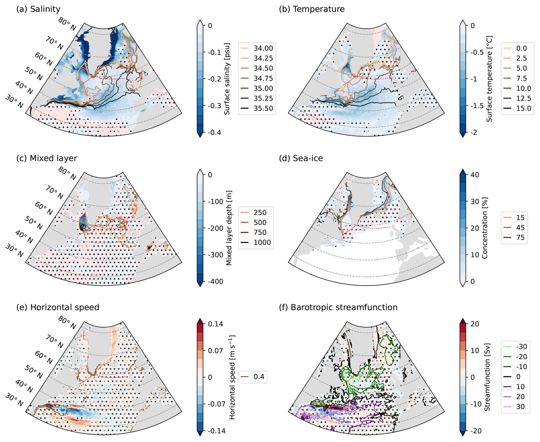
Figure 4 Response to the hosing in the last 10 simulated years for (a) annual surface salinity, (b) annual surface temperature, (c) March mixed layer depth, (d) DJF sea-ice concentration, (e) annual surface horizontal speed modulus, and (f) annual barotropic streamfunction in the North Atlantic; filled coloured contours represent the ensemble-mean anomalies of the hosing with respect to the reference control and the contour lines the climatology of the control. Non-significant values as identified by the bootstrap methodology are masked with dots to improve the visibility over the significant areas. Red dashed lines mark the OSNAP section. Figure B3 shows an enlarged view of the SPNA.

Sea surface temperatures (SST) also decrease over most of the SPNA and Norwegian Sea, especially along the sea ice edge, the western boundary currents, and the central SPNA (Fig. 4b). Unlike for SSS, no significant temperature changes are found in the northernmost latitudes of the Greenland coast, suggesting an absence of any local impact of the meltwater injection. By contrast, the southern Greenland coast and the closest sectors of the Labrador Sea do show significant cooling of up to 2 °C. Therefore, this confirms again the importance of the boundary-interior exchange in the Labrador Sea. As for SSS, we see a significant impact on the SSTs in the NAC, which cools down by about 1 °C. This cooling is unlikely to be driven exclusively by freshwater export from the Labrador Current, which shows a weaker SST response than the NAC region. Instead, it more likely reflects the impact of the already developed AMOC slowdown on the northward heat transport, which is explored further in Sect. 3.4.

The boundary currents around Greenland and the Labrador Sea experience a significant increase in speed (Fig. 4e). At the same time, sea ice concentration grows along the sea ice edge (Fig. 4d), which may be related to changes in northward heat transport (Ma et al., 2024), in the export from the Baffin Bay (Kwok, 2007; Våge et al., 2009; Schiller-Weiss et al., 2024) or persistent surface cooling due to strengthened stratification (Oltmanns et al., 2024).

The surface freshening in the interior Labrador Sea is accompanied by a statistically significant local shoaling of 200–400 m in the mixed layer (Fig. 4c). This is about a third of the local climatological mixed layer depth. The only other significant changes in the mixed layer depth occur along the boundary currents in the northeast and northwest of Greenland, although the anomalies are smaller. Interestingly, we note a lack of response in the Irminger and Nordic seas, the two other deep convection areas in the NH. This may be due to the lack of significant freshwater penetration, as previously mentioned. In addition, the Nordic Seas has very shallow climatological mixing due to a positive bias in sea ice (Martin-Martinez et al., 2025; Moreno-Chamarro et al., 2025), which limits the potential impact of the freshwater anomalies.

The shoaling in the mixed layer depth does not induce a clear deceleration in the Subpolar Gyre (SPG) strength (Fig. 4f), a connection that has been identified in previous studies (Moreno-Chamarro et al., 2017; Ghosh et al., 2023) that investigate the response to radiative-driven global warming. In our study, the expected deceleration of the SPG in response to the reduction in deep mixing may be counteracted by the acceleration of boundary currents caused by the strong freshwater-driven density gradient. However, the barotropic streamfunction shows significant changes over the Gulf Stream (Fig. 4f), characterised by a dipole with positive anomalies North of Cape Hatteras and negative anomalies South of Cape Hatteras. This pattern does not seem to be explained by a change in the position of the Gulf Stream, as no significant changes in the mean latitudinal position of the current is found when estimating its position from SST and sea surface height gradients (not shown). Instead, the dipole is consistent with a slowing down of the Gulf Stream (Fig. 4e) and with the patterns of change in surface temperature and salinity in the NAC (Fig. 4a and b). There is no significant change of the wind stress over the Gulf Stream, which excludes any driving role of the atmosphere on the Gulf Stream response (Fig. B4), which therefore may only be tied to a reduction in the deepwater mixing in the SPNA.

To investigate the impact of the freshwater hosing on the ocean subsurface we now focus our analysis on the two main sections where the water mass transport is being measured in the SPNA region, thanks to the collaborative international initiative OSNAP (i.e. Overturning in the Subpolar North Atlantic Program; Lozier et al., 2017). The OSNAP sections (red dashed lines in Fig. 4) cross several regions and currents of interest for our study: The Labrador Current, the Labrador Sea, the Greenland boundary currents, the Irminger Sea, the Reykjanes Ridge, and the Iceland Basin. We particularly focus on the changes in mixed layer depth, practical salinity, potential temperature, and potential density across the SPNA (Fig. 5). For the OSNAP section, the reduction in mixed layer depth is only significant in the Greenland and Labrador currents and parts of the interior of the Labrador basin (Fig. 5a).

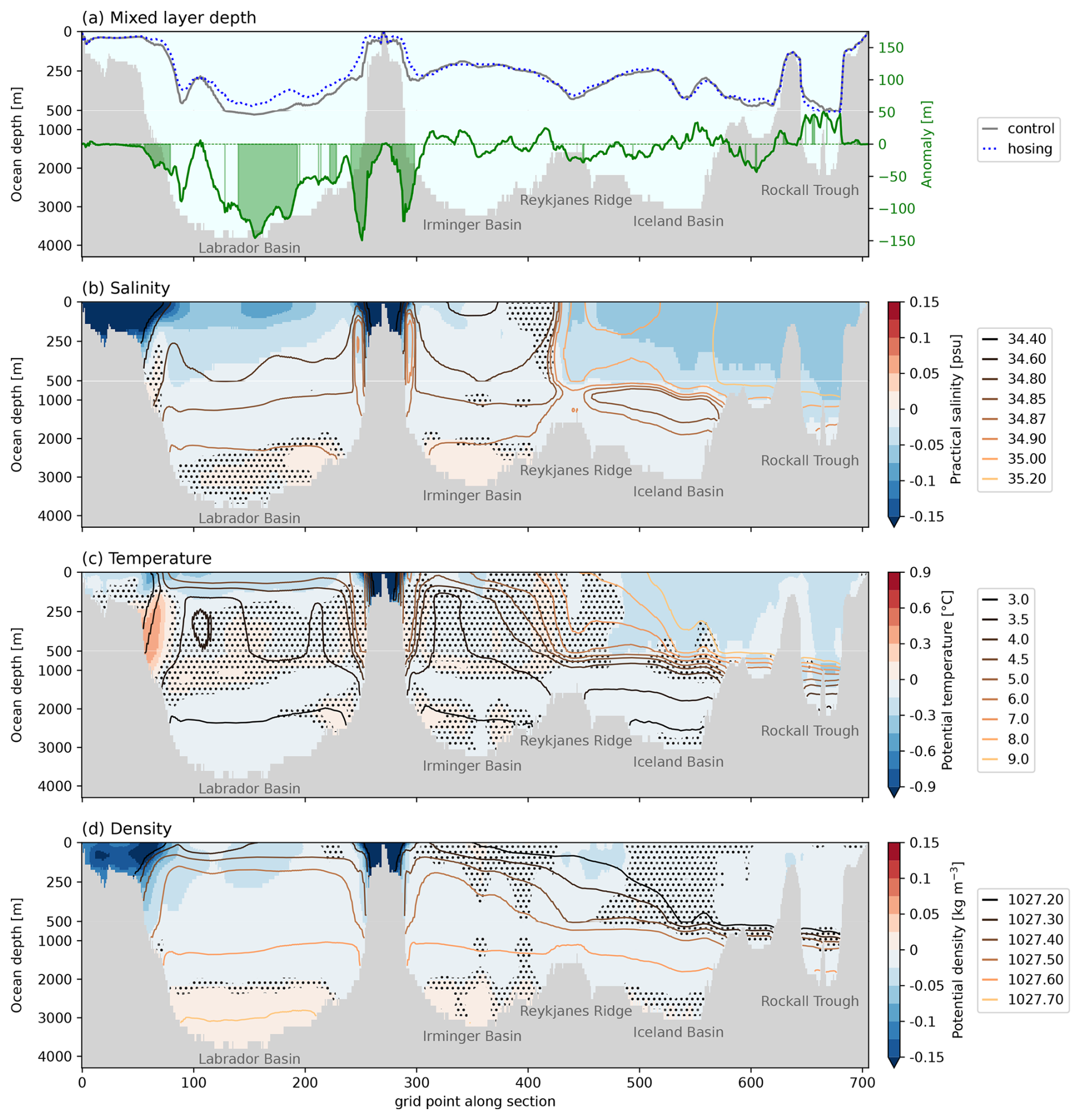
Figure 5 Response to the hosing in the last 10 simulated years for the (a) mixed layer depth, (b) potential temperature, (c) practical salinity, and (d) potential density across the OSNAP section (see red lines in Fig. 4); in (a) anomalies are filled (green) when they are significant by the bootstrap methodology; in (b)–(d) filled coloured contours represent the ensemble-mean anomalies of the hosing with respect to the reference control and the contour lines the climatology of the control. Non-significant values as identified by the bootstrap methodology are masked with dots to improve the visibility over the significant areas.

The meltwater fluxes induce statistically significant fresher conditions above 2000 m for almost the whole OSNAP area (Fig. 5b). As expected, the water is much fresher over the continental shelves of Greenland and Newfoundland, where the boundary currents are located, but there is also a clear penetration of freshwater anomalies into the Labrador Sea interior. In the top 200 m, practical salinity is reduced by about 0.075 psu, followed by a reduction of about 0.05 psu down to 500 m, and a slight significant reduction down to 2000 m. The Deep Western Boundary Current (DWBC), which is located in the western boundary of the Labrador basin at around 500 m depth, does not show a significant change in practical salinity. The intensity of the freshening in the eastern side of the SPNA, east of the Reykjanes Ridge, is similar to that in the Labrador Sea but a bit lower. The freshening anomalies in this area follow the isopycnal structure (see contours in Fig. 5d), suggesting a prominent role of the along-isopycnal transport by the SPG circulation.

The temperature response is more localized than for salinity. There is significant cooling over the Greenland shelf, by more than 1 °C, and also but not so strong in the Labrador Current (Fig. 5c). Potential temperatures in the upper 200 m of the Labrador Sea interior and the eastern side of the SPNA are about 0.2 °C colder in the hosing experiments. However, the most interesting result regarding potential temperature changes happens in the DWBC where there is a significant warming of about 0.3 °C while no significant changes in salinity occur. We hypothesize that reduced deep-water mixing in the Labrador Sea could lead to reduced DWBC feeding. This would not only reduce the SPNA AMOC, but also warm the current. This hypothesis is explored further in the water mass transformation analysis in Sect. 3.3.

There is a general reduction of density in the upper 2000 m (Fig. 5d). Once again, the Greenland and Labrador currents show the greater changes, with the density gradient increasing towards the interior and accelerating the currents. This is consistent with previously published results (Schiller-Weiss et al., 2024). The density loss in the boundary currents exceeds 0.15 kg m⁻³; whereas in the surface waters of the Labrador Sea interior and over the Reykjanes Ridge, the density anomaly is smaller than 0.05 kg m⁻³. These density anomalies are driven by salinity changes, as expected. In other parts of the OSNAP section (e.g. the surface waters of the Irminger Sea and the Iceland Basin), temperature-driven changes compensate for those of salinity, resulting in no clear density response. In contrast, there is no significant salinity response in the DWBC, but rather a positive temperature anomaly, which drives the density anomaly there.

3.3 Water mass transformation

To better understand the impact of fresh-water driven changes on the AMOC, we have carried out a surface forced water mass transformation (SFWMT) analysis. Figure 6 shows the freshwater and heat contributions to the buoyancy forcing, as in Eq. (1) from Petit et al. (2023), for the last 10 years of the hosing. The freshwater forced water mass transformation (WMT) shows a negative signal on the coast of Greenland, as expected from the effect of the injected freshwater. However, a concurrent increase in sea ice extent (see Fig. B3) produces a positive signal due to the brine rejection. This gives rise to a dipole-like pattern along the eastern coast of Greenland. The central and eastern Labrador Sea also shows a small haline contribution to buoyancy loss.

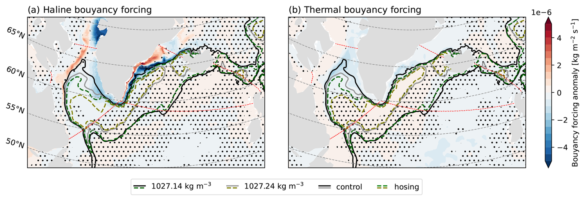
Figure 6 Response to the hosing in the last 10 simulated years for the (a) freshwater flux and (b) heat flux contributions to SFWMT; filled coloured contours represent the ensemble-mean anomalies of the hosing with respect to the reference control. Contour lines show the surface 1027.14 and 1027.24 kg m⁻³ isoline in control (black, grey) and hosing (green, olive). Non-significant values as identified by the bootstrap methodology are masked with dots to improve the visibility over the significant areas. Red dashed lines mark the limits for the analysis in Fig. 7.

The thermal contribution to the buoyancy forcing is reduced in the hosing runs across both sides of Greenland, extending further into the northern Labrador Sea. The reduction in the eastern side of Greenland seems to be related to the sea ice increase. The magnitude of these temperature-driven changes is, however, comparably smaller than haline-driven ones. More broadly, both haline and thermal changes in the SFWMT are likely not driven directly by the local surface buoyancy forcing, but rather by the reduction in surface density that develops when the injected freshwater is advected into the Labrador Sea interior (see below). Additionally, there is a small but statistically significant positive signal in the thermally driven buoyancy forcing in the Irminger Sea for the water masses denser than 1027.24 kg m⁻³.

We divide our analysis into the West and East regions, bounded in the south by the respective OSNAP sections and to the north by the straits connecting to the Baffin and Hudson bays (BHB) and the Greenland-Scotland-Ridge (GSR), respectively (red dashed lines in Fig. 6). Figure 7a–b and e–f shows the volume overturning streamfunction across the boundary sections. The strongest response is a reduction in the net transport of light waters ($<\mathrm{1026.25}\mathrm{kg}{\mathrm{m}}^{-\mathrm{3}}$) in OSNAP-West, driven by an intensification of the freshwater input by the Greenland Current into the Labrador basin that is not compensated by the Labrador Current outflow. Indeed, the resulting change in the light water transport is partly compensated by exchanges through the Baffin Bay (shown aggregated to Hudson Bay in Fig. 7b, whose contribution is negligible). A similar compensation happens for light waters in OSNAP-East, where the transport response is compensated by boundary current exchanges across the Denmark Strait (shown aggregated to the Iceland-Scotland Ridge in Fig. 7f). Both OSNAP-West and OSNAP-East also show a reduction in the dense water exports: the maximum transport is reduced from 4.3–2.7 in the west Sv and from 15.4–14.7 Sv in the east (Table 1). The eastern side dominates the total OSNAP transport, but the stronger reductions occur in the western section, following the forced changes in the Labrador Sea.

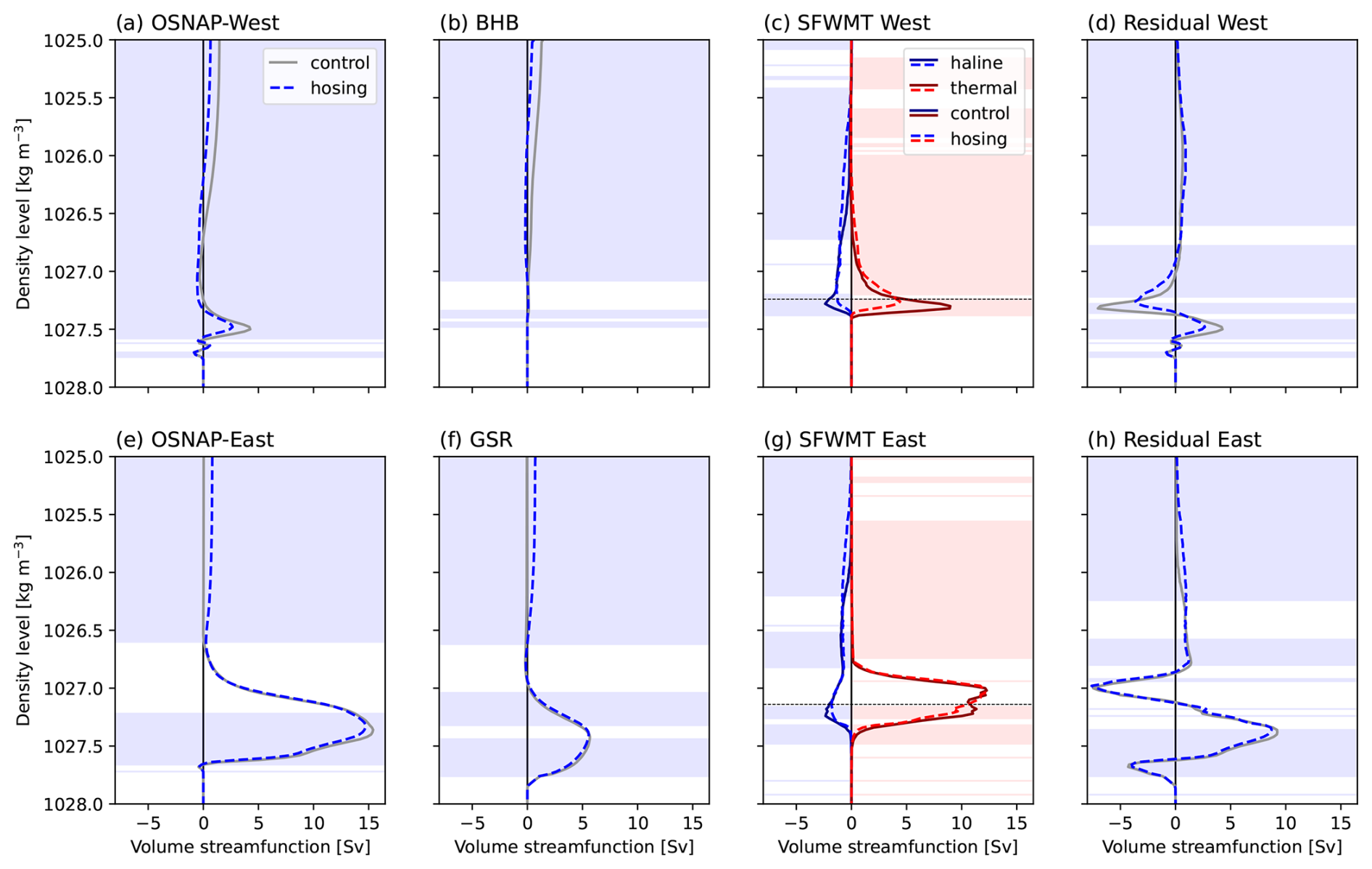
Figure 7 Response to the hosing in the last 10 simulated years for the overturning streamfunction in density space in (a) OSNAP-West, (b) BHB, (e) OSNAP East, (f) GSR; values in the hosing (blue) and control (grey) ensembles. Thermal (blues) and haline (reds) contributions to the SFWMT in the (c) West and (g) East regions. Residual WMT computed as the net transport out of the region minus the total SFWMT for (d) West and (h) East. The transport values are positive for the water masses entering the region for both (b) BHB and (f) GSR, and positive for the water masses leaving the region for (a), (e) OSNAP sections. Therefore, the net transport out of the regions are equal to OSNAP-West minus BHB and OSNAP-East minus GSR. The positive values in (c)–(d), (g)–(h) represent water creation while negative values represent water mass destruction. The ensemble means are shown by lines, the background is coloured when the anomalies are deemed statistically significant by the bootstrap methodology. The lines in (c), (g) represent the 1027.24 and 1027.14 kg m⁻³ density levels, respectively, which isolines are plotted in Fig. 6.

Table 1 Maximum value of the volume overturning streamfunction in density space across both OSNAP transects for the last 10 years of the hosing.

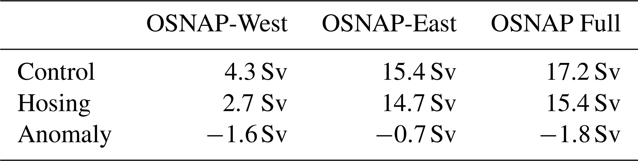
The injected freshwater produces a negative anomaly in the haline contribution to the SFWMT for light density waters in both regions. However, for denser waters there is a reduction in the absolute magnitude both for the haline and thermal contributions, resulting in a positive anomaly in the haline contribution and a negative anomaly in the thermal contribution. Both reductions are statistically significant for waters denser than 1027.24 kg m⁻³ in the western region and 1027.14 kg m⁻³ in the eastern region (see horizontal lines in Fig. 7c and g). For the western region, the buoyancy forcing within the 1027.24 kg m⁻³ isoline is slightly negative for the haline contribution and not significant for the thermal contribution (see Fig. 6). For the eastern region, the buoyancy forcing enclosed by the 1027.14 kg m⁻³ isoline is not significant for the haline contribution and slightly positive for the thermal contribution. Therefore, the response in the SFWMT profiles cannot be attributed to changes in surface forcing itself, and rather to the reduction of the area enclosed by the respective density isolines, which leaves less water available for transformation at those density levels. The changes in SFWMT are thus explained by the lightening of the surface waters due to the direct freshwater injection.

The changes in the residual part, which represents densification by diapycnal mixing in addition to errors derived from the offline computation, reflect the reduced availability of waters for transformation from about 1027.25–1027.5 kg m⁻³ in the western region, (Fig. 7d), due to the stronger reduction in the thermal compared to the haline SFWMT contribution. This also explains the reduction in the transport through the OSNAP-West section. Meanwhile, the changes in the mixing in the eastern region are modest, as the absolute reductions in both contributions (which have opposite signs) are almost equivalent and all relatively much smaller. The thermally-driven reduction in SFWMT at OSNAP-West implies that less surface-cooled waters mix down to higher densities to feed the DWBC, which in turn explain the relative temperature increase for those waters seen in Fig. 5.

3.4 Time evolution

We now study the time evolution of some key indices from the beginning of the experiments, to understand how the different changes described in the previous Section develop. Figure 8 shows the regions we have used to define the different indices. These regions have been selected taking into account the topography, the position of key ocean currents, and main deep mixing areas. Since, for a given time step, it will be difficult to measure significance based solely on three data points (i.e. the ensemble members), we will pay particular attention to those changes for which the three members are consistent in sign for at least three consecutive years.

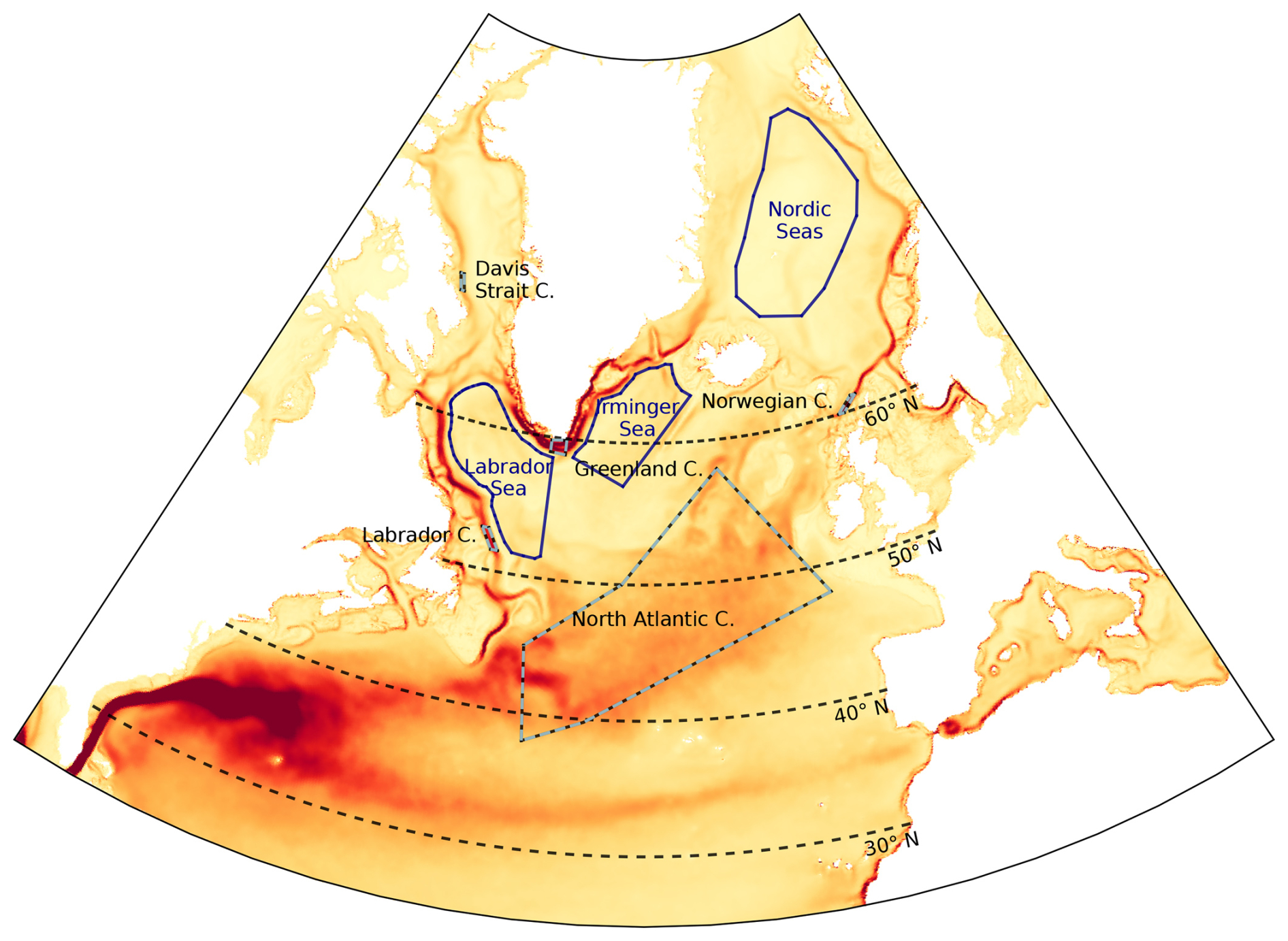
Figure 8 Areas used for the time series in Fig. 9. The background represents the average of horizontal speed modulus during the last 10 years in the hosing experiments.

The Greenland Current exhibits a rapid response in surface salinity and temperature (Fig. 9a and b). The average salinity reduction for the whole period is of about 0.40 psu, while the temperature reduction is of around 0.94 °C. Among the selected regions, the Greenland Current presents the most immediate response, as it is directly exposed to the meltwater forcing. Farther downstream, the Labrador Current (Fig. 9a) shows consistent changes with the Greenland Current from the beginning of the experiments, although the anomalies are only consistent across members after the first year. Nevertheless, these changes are significantly less intense than for the Greenland Current, with a salinity loss of around 0.15 psu and a temperature drop of approximately 0.2 °C. One possible cause of this could be the horizontal mixing of negative salinity anomalies from the Greenland Current as they circulate around the Labrador Sea. At the same time, the stronger winter sea-ice growth under the hosing could also contribute to the salinity of the current as it advances due to brine rejection. It is evident that both currents have also accelerated since the beginning of the freshwater hosing (Fig. 9c) Also, in both currents, while the temperature and salinity response show a rapid adjustment during the first years of hosing, the current acceleration exhibits a more gradual increase. The initial speed-up is consistent with a fast geostrophic response to the enhanced cross-current density gradient, while the longer-term trend likely reflects progressive subpolar gyre adjustments driven by ocean–atmosphere feedbacks (e.g. Oltmanns et al., 2020).

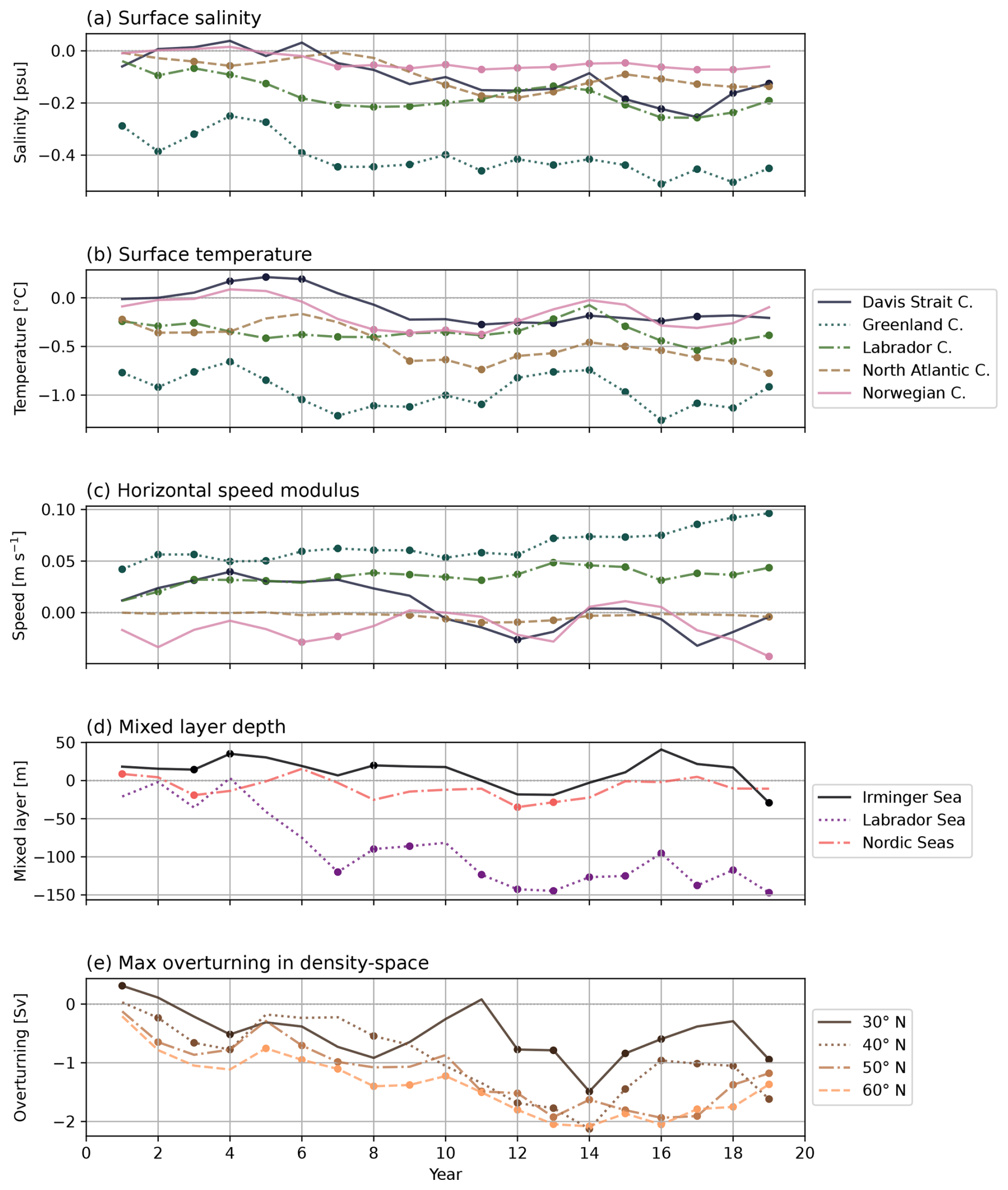
Figure 9 Time series of ensemble-mean anomalies due to the hosing with respect to the reference control for (a) annual surface salinity, (b) annual surface temperature, (c) annual surface horizontal speed modulus, (d) march mixed layer depth, and (e) annual maximum overturning in density space. The areas used in (a)–(d) are shown in Fig. 8. All the data is filtered with a 3 years moving average. Dots denote the points where the difference of the three members agree in the sign.

The Davis Strait Current, located in the Baffin Bay northwest of the Labrador Sea, shows much weaker changes, with little consistency and persistence in time both for the speed and the temperature changes. At the same time, its salinity decreases progressively, with sign-consistent anomalies over the last 5 years of the simulations (marked by dots). Therefore, the changes in this current may respond to the accumulated freshwater in the Baffin Bay coming from the neighboring Greenland coast. At the opposite end of the Arctic-Atlantic sector, the Norwegian Current – which represents an inflow into the Arctic – experiences a consistent freshening after year 8. The long lag for these salinity changes to emerge compared to the other currents could be explained by the time required by the mean circulation in the SPNA to carry the freshwater anomalies formed near Greenland to that region, although they could also be explained by a delayed SPG weakening and its effects on the northward transport of salt. This second hypothesis, however, is not supported by the barotropic streamfunction, which does not show a clear large-scale reduction in the SPG (Fig. 4f), suggesting that the transport of freshwater anomalies by the mean SPNA circulation is the most likely cause of the Norwegian Current freshening.

A consistent freshening and cooling of the NAC region also takes place after year 11. This coincides with the time at which the overturning circulation shows a consistent drop of more than 1 Sv at 40, 50 and 60 ° N (Fig. 9e). Therefore, the changes in the NAC region may just emerge in response to the reduction in the northward transport of warm and saline waters due to the large-scale AMOC slowdown, as the AMOC weakening and Labrador Sea mixed layer shoaling emerge consistently around year 7 at subpolar latitudes (60° N, Fig. 9d and e), prior to the NAC freshening and cooling. This particular response may trigger a feedback that further reduced salinity in the whole SPNA, as it has already been described in several studies (Drijfhout et al., 2011; Jackson, 2013; Liu et al., 2014). Other processes could also contribute, such as the direct advection of fresh, cool waters by the SPG or changes of the air–sea fluxes. The horizontal speed in the NAC region shows a consistent reduction between years 10 and 15, and, although the mean anomaly remains negative thereafter, the ensemble members no longer agree on the sign anomaly.

To understand the changes in the overturning streamfunction we now focus on the mixed layer depth changes. Only the Labrador Sea mixed layer depth is permanently reduced after year 6, in contrast to the Irminger and Nordic Seas (Fig. 9d) where no consistent changes are observed. Both the Irminger and Nordic seas have shallow mixed layers in the control experiment, 310 and 120 m on average, the Labrador Sea being the main site of deep convection in the SPNA in EC-Earth3P-VHR simulations (Martin-Martinez et al., 2025), with an average mixed layer depth of 480 m. In the Labrador Sea, the reduction becomes consistent in sign from year 7 onwards, with an average reduction of 100 m. The changes in the mixed layer depth seem to lead by 2–4 years the changes in the maximum overturning streamfunction at 40 and 50 ° N, but lag by 2 years the AMOC changes at 60° N. At 60° N, the fastest response is consistent with a circulation adjustment because the freshwater anomalies remain largely confined within the boundary currents, maintaining a strong cross-current density gradient with the denser interior. By the time they reach 40–50° N, the freshwater anomalies have spread more broadly into the subpolar gyre interior, reducing the cross-current gradient, and the overturning response is more dominated by the reduction in deep convection in the Labrador Sea, which acts on a longer timescale. The signal does not reach 30° N with the same intensity, and it is only consistent for years 12–16. We note that Martin-Martinez et al. (2025) showed that the eddy-rich version of the model exhibits weaker meridional connectivity of AMOC anomalies across latitudes compared to lower-resolution configurations, which may partly explain why the signal does not propagate southward to 30° N with the same intensity and persistence.

To better explore the changes in the Labrador Sea, we show the Hovmöller diagrams of the spatial averages of practical salinity, potential temperature, and potential density (Fig. 10) in the Labrador Sea interior as a function of time and depth. It is worth noting that the vertical structure of the climatological Labrador Sea temperature and salinity is more realistic in the eddy-rich configuration than in the eddy-parameterised version of the model (Martin-Martinez et al., 2025), which provides greater confidence in the simulated response. For the three variables, changes are stronger in the upper 200 m than below. The salinity changes are not fully consistent in time nor across the ensemble members during the initial 7 years. In fact, during these years, there is a competition between the salinity and temperature anomalies – which are consistently negative throughout the whole period – to drive the changes in density, which results in a succession of positive (when temperature dominates) and negative (when salinity dominates) changes at the surface. This competition between opposing salinity and temperature contributions likely explains the delayed emergence of a consistent negative density signal in the upper ocean. From the year 7 onwards, salinity changes completely dominate the changes in density in the upper 500 m of the Labrador Sea interior. This happens at the same time that consistently negative anomalies in the mixed layer depth start developing (Fig. 9d). Although heat loss to the atmosphere could contribute to the early surface temperature response in the Labrador Sea interior, it does not appear to be the dominant driver (not shown). We hypothesize that the fast temperature drop arises because lateral heat advection is more efficient than the advection of salt/freshwater anomalies, which are more susceptible to dilution and mixing along the boundary current, therefore requiring several years of cumulative transport before significantly impacting interior salinity.

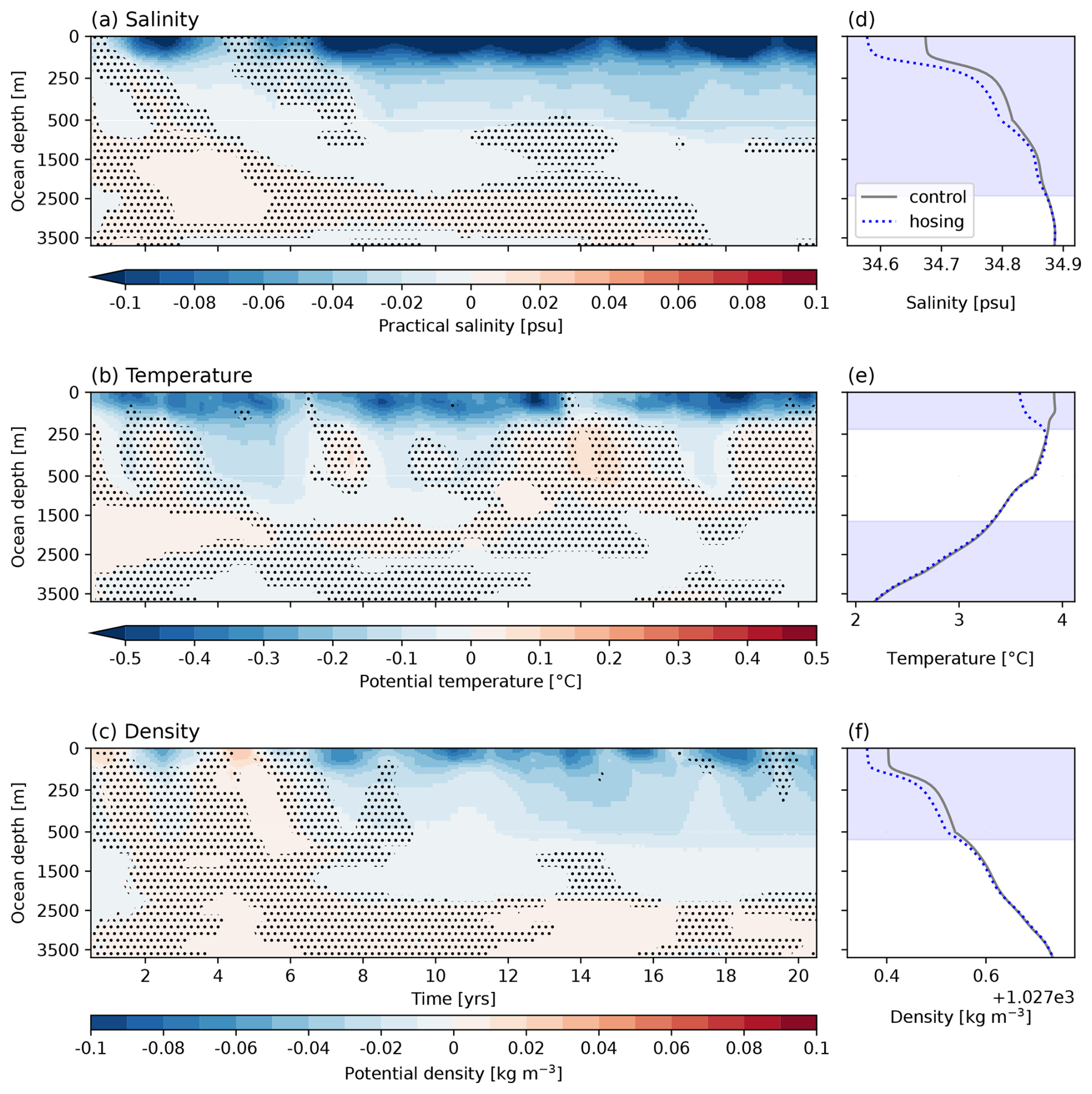
Figure 10 Depth vs. time Labrador Sea interior ensemble-mean anomalies in (a) salinity, (b) temperature and (c) density as computed between the hosing and the reference control. The anomalies are computed as 12 month moving averages. Anomalies that are not fully consistent in sign between the three ensemble members are masked with dots to highlight the visibility of the fully consistent ones. Vertical profiles of the spatially averaged DJF Labrador Sea interior (d) salinity, (e) temperature and (f) density values in the hosing (blue) and control (grey) ensembles during the last 10 years of the simulations. The ensemble means are shown by lines, the background is coloured when the anomalies are deemed statistically significant by the bootstrap methodology.

The mixed layer depth response can be explained by a change in the stratification of the Labrador Sea, as the freshwater accumulates mainly at the surface, increasing the vertical salinity gradient, which leads to a more stratified density distribution in the later years when salinity dominates the density signal (Fig. 10d). The density changes induced by the potential temperature vertical profile oppose those induced by salinity (Fig. 10e), without fully counterbalancing them (Fig. 10f). These results support a weakening response of Labrador Sea interior deep water mixing to the quasi-realistic Greenland meltwater forcing mediated via freshwater exchanges from the boundary currents. The spatial distribution of the forcing appears to play an essential role in this pathway: freshwater injected close to the boundary current system is efficiently transported along the SPG boundary and can reach the Labrador Sea convection region, whereas forcing applied far from these pathways may have a very different or even opposite effect. This is illustrated by Wei and Zhang (2024), who produce a contrary response when injecting freshwater only in the south of the Nordic Seas, and by Ma et al. (2024), who show that among four injection regions in the North Atlantic, freshwater applied in the Irminger Basin, which is directly upstream of the Labrador Sea along the boundary current, is the most effective at suppressing deep convection there. Idealised experiments applying uniform forcing across the North Atlantic, such as Jackson et al. (2023), may therefore not capture the spatially selective nature of this mechanism and could produce a less realistic representation of SPNA dynamics.

3.5 Global impacts

We extend our analysis to the global impacts in our hosing simulations, acknowledging that the limited length of our simulations (21 years) and the moderate but consistent AMOC weakening might not be sufficient to drive large-scale, strong impacts on the global climate. To study these global impacts, we examine changes in the atmospheric surface temperature, sea level pressure, and precipitation. Figure 11 shows the freshwater hosing-driven anomalies in these three variables over the last ten years for the months of December–January–February (DJF, boreal winter or austral summer) and June–July–August (JJA, austral winter or boreal summer).

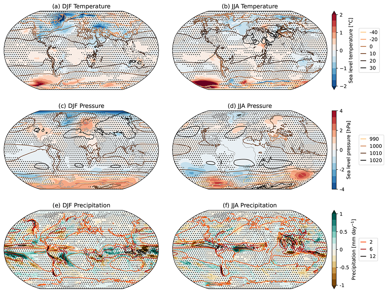
Figure 11 Response to the hosing in the last 10 simulated years for (a, b) atmospheric surface temperature, (c, d) sea level pressure, and (e, f) precipitation, for (a–e) DJF and (b–f) JJA; filled coloured contours represent the ensemble-mean anomalies of the hosing ensemble with respect to the reference control and the contour lines the climatology of the control. Non-significant values as identified by the bootstrap methodology are masked with dots to improve the visibility over the significant areas.

The most intense surface air temperature changes occur over the ocean during boreal winter (Fig. 11a). During this season local surface air temperatures drop by more than 5 °C to the north-east of Baffin Bay and by about 2.5 °C in the Greenland Sea close next to Svalbard (see Fig. B6). The anomalies to the north-east of Baffin Bay are significant throughout the whole year (not shown), reaching maximum strength during winter. There is also a slight consistent cooling in most of the SPNA and Greenland. These negative changes in atmospheric surface temperature are linked to similar changes in SST (Fig. 4b). Over the continents, the most clear signal is a widespread cooling from the Eastern Mediterranean to the Middle East. During the austral winter the strongest response happens in the SH (Fig. 11b), with a strong warming (more than 5.5 °C) over the Amundsen and Ross Seas, near West Antarctica, which also occurs but weaker in the austral summer. Due to the short time of integration, these anomalies are most probably caused by an atmospheric teleconnection rather than to adjustments in ocean heat transport.

Similar positive temperature anomalies in the Amundsen Sea are described by Diamond et al. (2025) in an analysis focused on NAHosMIP runs. These remote Southern Hemisphere anomalies are consistent with a poleward-propagating Rossby wave train forced by anomalous tropical heating associated with the AMOC weakening, a mechanism that is discussed further down in the context of the sea level pressure response. The main signals in the boreal summer in the NH are a widespread cooling in the SPNA (of smaller amplitude than for winter) and a warming in the Western Mediterranean. Overall, the described anomalies in the NH and SH are consistent in sign during summer and winter. However, the summer anomalies tend to be weaker in magnitude, usually less than half the intensity of the winter ones, in particular in the deep convection areas of the Labrador and Ross seas, where the winter mixing response might reinforce the temperature signals.

The sea level pressure response is most prominent in the polar regions. During DJF, the polar low gets reinforced (Fig. 11c), with a local minimum also observed over the Labrador Sea accompanied by two anomalous high pressure systems over Central North America and Europe. The anomalous high over Europe is consistent with a deflection of the westerlies that could be driving northerly cold-air advection into the Eastern Mediterranean, contributing to the observed cooling there. We also see positive high pressure anomalies in most of the Antarctic Circle, opposed by negative anomalies in the Pacific sector of the Southern Ocean. These changes are consistent with a positive Northern Annular Mode (NAM)-like response in the NH and a negative Southern Annular Mode (SAM)-like response in the SH. The NAM response could be reinforcing the cooling over the Labrador Sea, as it is consistent with an intensification of the westerlies over that region, while counterbalancing effect might be happening between SAM and the cooling signal over the Southern Ocean, as negative SAM phases tend to weaken the westerlies and their forcing on the ocean surface.

During JJA, the responses in sea level pressure are weaker than for DJF in the NH (Fig. 11d). There is a consistent increase in sea level pressure over the central North Atlantic region and a decrease over Greenland. This spatial pattern is roughly consistent with a positive summer North Atlantic Oscillation (NAO)-like response, a pressure pattern that has been shown to be more frequent under larger hosing experiments (Bellomo et al., 2023). Positive responses are also observed over the Urals and West Siberia. In the SH, there is a big negative response in the Southern Pacific and Southern Atlantic regions and large positive responses south of Australia and over the Amundsen Sea. This last change could explain the positive temperature anomaly highlighted above for the same region and season, as the warming is located to the west of the sea level pressure anomaly, where warm southward advection is expected. These changes could be induced by a Rosby-wave train originating in Central America and propagating eastward into the Southern Ocean, as described in Diamond et al. (2025), generating sea level pressure and temperature anomalies with regional asymmetry.

Regarding precipitation in DJF, we see a consistent increase south of the Equator, both in the Pacific and Atlantic basins (Fig. 11e), which could be indicative of a southward migration of the ITCZ. However, the precipitation signal is more regionally confined than show in other models in response to stronger AMOC weakenings (Jackson et al., 2015; Liu et al., 2020; Orihuela-Pinto et al., 2022; Bellomo et al., 2023; Ma et al., 2024). This suggests that the amplitude of the ITCZ shift scales with the magnitude of the AMOC weakening. Also, a more detailed analysis with diagnostics that characterises its latitudinal shifts and intensity at the global scale (as in Santos-Espeso et al., 2025) does not reveal a consistent ITCZ response (not shown). We also notice a precipitation increase in the equatorial Atlantic during JJA (Fig. 11f) and a decrease in the Amazonas basin and the Maritime continent in DJF.

4 Conclusions

This paper explores the impact of applying a quasi-realistic Greenland meltwater forcing in the Subpolar North Atlantic (SPNA) region, the Atlantic Meridional Overturning Circulation (AMOC), and the global climate. To that end, we use the HighResMIP coupled global model EC-Earth3P-VHR, which has an eddy-rich ocean grid (about 8 km in the mid-latitudes), to run a three-member ensemble of 21 year long freshwater hosing experiments, branching from different AMOC states of a 1950-control simulation. The magnitude of the forcing corresponds to 0.0419 Sv of freshwater on annual average, with a temporal and spatial distribution around Greenland derived from a product based on observations and model simulations. The additional freshwater is added on top of the coupled model river runoff and iceberg calving fluxes. The hosing experiments share the same perpetual 1950 radiative forcing conditions as the control simulation, ensuring that the simulated responses can be unambiguously attributed to the freshwater forcing.

We find the following responses to the Greenland freshwater hosing:

• A broad weakening of the AMOC across the 10–65° N latitude band, averaging 1.3 Sv (10.0 %) in the 1027.4–1027.6 kg m⁻³ density range by the end of the experiments, with a peak reduction of 3.0 Sv (19.9 %) at 60.2° N where the subpolar signal is strongest. This is a substantial reduction given the relatively short duration and moderate magnitude of the applied forcing. In depth space, the response is weaker, with a basin-wide average reduction of 0.7 Sv (6.5 %) between 500–1000 m and a maximum weakening of 1.4 Sv (8.6 %) at 33.8° N.

• A general surface freshening and cooling spanning across the SPNA. While the changes along the boundary currents and the interior Labrador Sea seem to directly emerge in response to the freshwater forcing, the changes in the eastern SPNA seem to be linked to a reduction in the northward transport of salty and warm waters, driven by the slowdown of the AMOC.

• In the first year, the freshwater fluxes induce an acceleration of the boundary currents around East and West Greenland, which drives the local cooling. Over the following years, freshwater anomalies gradually penetrate into the Labrador Sea interior, where they start reducing the vertical mixing by year 7. The AMOC experiences a first rapid weakening in the SPNA through circulation adjustments to the density signals emerging along the boundary current, a weakening that is enhanced and becomes more widespread as the Labrador Sea's capacity to produce denser waters is progressively reduced. The weakening of deep convection reduces the supply of cold, dense waters to the Deep Western Boundary Current (DWBC), resulting in a relative warming of DWBC waters at the OSNAP section.

• At the global scale, only a few regions experience significant impacts within the relatively short duration of the experiment. We highlight the development of a positive phase of the Northern Annular mode and a negative phase of the Southern Annular mode in DJF, which respectively cause a cooling over Western Europe and a warming over the Amundsen and Ross Seas. Typical impacts previously linked to strong AMOC reductions in freshwater hosing experiments, like a southward Intertropical Convergence Zone (ITCZ) shift, are not reproduced in our relatively short experiments. In general, these atmospheric signals are less robust than the identified ocean signals described earlier.

The fidelity of the spatio-temporal distribution of the injected meltwater fluxes and the model capacity to resolve mesoscale ocean processes are two key aspects of our study, both jointly expected to enhance the realism of the simulated responses. Compared to eddy-parameterised models, the higher ocean resolution has enabled a more realistic representation of the narrow boundary currents that quickly carry the freshwaters southward around Greenland, and of the mesoscale eddies that govern the lateral exchanges with the interior of the Labrador Sea (Georgiou et al., 2020; Schiller-Weiss et al., 2024) while keeping the Irminger Sea interior isolated. In the hosing experiments, the water mass transformation analysis has shown that the AMOC weakening is driven by a reduction in dense water formation confined to the Labrador Sea, with the Irminger and Nordic Seas showing no significant convective response, a regional selectivity that reflects the model's capacity to resolve the eddy-driven boundary-interior exchanges that control how the injected freshwater reaches the deep convection region. The stronger role of the Labrador Sea in dominating AMOC variability has also been discussed in other studies, e.g. Yeager et al. (2021). Further south, the eddy-rich configuration enables a more accurate Gulf Stream separation, as shown in other studies (Marzocchi et al., 2015; Moreno-Chamarro et al., 2021; Frigola et al., 2025), and sharper frontal gradients, with important implications for the responses in the northward heat and salinity transports and the atmospheric circulation aloft.

Interestingly, the local response detected in the SPNA in our experiments aligns with that found by Schiller-Weiss et al. (2024), who used a global configuration of the ocean/sea-ice NEMO model with a finer horizontal resolution of $\mathrm{1}/\mathrm{20}$° in the North Atlantic, where they studied the response of the SPNA to the 1997–2021 enhanced Greenland melting. While the simulation length is broadly comparable to ours (25 vs. 21 years), their freshwater anomaly (derived from the observed post-2000 acceleration of Greenland melt relative to the pre-2000 climatology) is substantially weaker than the constant 0.0419 Sv perturbation applied here. We further highlight that the qualitative ocean response appears robust across different initial AMOC states, although quantitative differences remain. The atmospheric responses tend to show larger differences across members, which suggests that longer experiments might be needed for them to emerge more robustly, like the typical southward shift of the ITCZ (Jackson et al., 2015; Liu et al., 2020; Orihuela-Pinto et al., 2022; Bellomo et al., 2023; Ma et al., 2024), which might require a stronger or more persistent in time AMOC response. Likewise, a new coordinated protocol to assess the sensitivity of the AMOC to the projected Greenland ice sheet melting tailored to eddy-rich climate model configurations is warranted to determine the inter-model consensus and main underlying uncertainties in the AMOC response, which is key to better understand its future evolution. The Tipping Points Modelling Intercomparison Project (TIPMIP; Winkelmann et al., 2025) could define and coordinate this protocol, building on the experimental frameworks put forward by the High-Resolution Model Intercomparison Project phase 2 (HighResMIP2; Roberts et al., 2025).

Appendix A: Estimation of the temperature

Due to a failure in the data storage, many global 3D temperature data files were lost. Therefore, Fig. B5 shows an estimate of the temperature instead of the model output. The estimation was performed using an approximation based on constant coefficients of thermal expansion (α) and salinity contraction (β). Given the relation in Eq. (A1):

$$\begin{array}{}\text{(A1)}& \mathrm{d}\mathit{\rho }={\mathit{\rho }}_{\mathrm{0}}(\mathit{\beta }\mathrm{d}S-\mathit{\alpha }\mathrm{d}T)\end{array}$$

we can linearly approximate the temperature as shown in Eq. (A2):

$$\begin{array}{}\text{(A2)}& T=T_{\mathrm{0}}+{\displaystyle \frac{\mathrm{1}}{\mathit{\alpha }}}\left(\mathit{\beta }(S-S_{\mathrm{0}})-{\displaystyle \frac{\mathit{\rho }-{\mathit{\rho }}_{\mathrm{0}}}{{\mathit{\rho }}_{\mathrm{0}}}}\right)\end{array}$$

we have taken the coefficients from Nycander et al. (2015) suggested by Vallis (2006); $\mathit{\alpha }=\mathrm{1.67}\times {\mathrm{10}}^{-\mathrm{4}}{\mathrm{K}}^{-\mathrm{1}}$, $\mathit{\beta }=\mathrm{7.8}\times {\mathrm{10}}^{-\mathrm{4}}{\mathrm{psu}}^{-\mathrm{1}}$, T₀=10 ° C, S₀=35 psu, ${\mathit{\rho }}_{\mathrm{0}}=\mathrm{1027}\mathrm{kg}{\mathrm{m}}^{-\mathrm{3}}$.

Note that the relation in Eq. (A1) is non-linear, as α is defined at constant salinity and β at constant potential temperature. Therefore, the estimated temperature resulting from Eq. (A2) is not exact. However, a test in the OSNAP section (not shown) shows that the estimated temperature anomalies tend to be weaker than the true model outputs. Nevertheless, the sign and significance of the anomalies remain consistent in both cases.

Appendix B: Supplementary figures

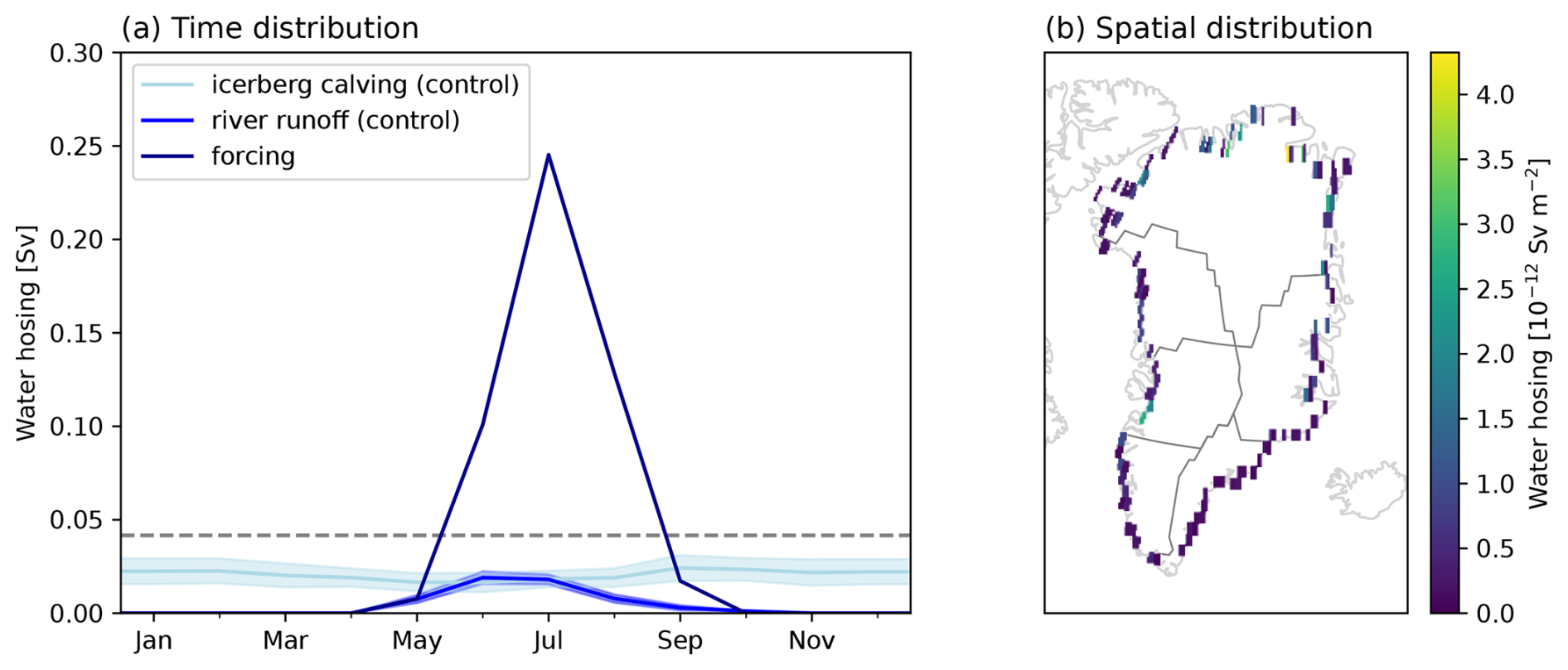
Figure B1 (a) Total monthly freshwater forcing time distribution, monthly climatologies of river runoff and monthly climatologies of iceberg calving fluxes and (b) annual averaged freshwater forcing runoff spatial distribution. Forcing values are those given to the model as an input. The dashed line in (a) indicates the annual average of the forcing. The shadow areas in (a) represent the standard deviation of monthly river runoff and iceberg calving fluxes. The grey lines in (b) indicate the separation between the six sub-drainage basins.

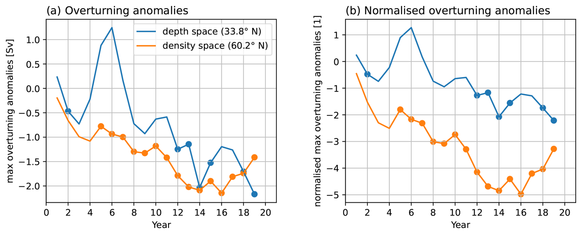
Figure B2 Maximum volume overturning streamfunction and in the Atlantic basin for (a) annual data with 3 year moving average and (b) annual data with 3 year moving average divided by the control 3 year moving average's standard deviation. The values have been computed with annual averages and filtered with a 3 year moving average. The latitudes were selected where the corresponding maximum change in the last 10 years happens, see Fig. 3. The gray dots show the annual average maximum volume of the overturning stream function in the control during the first year.

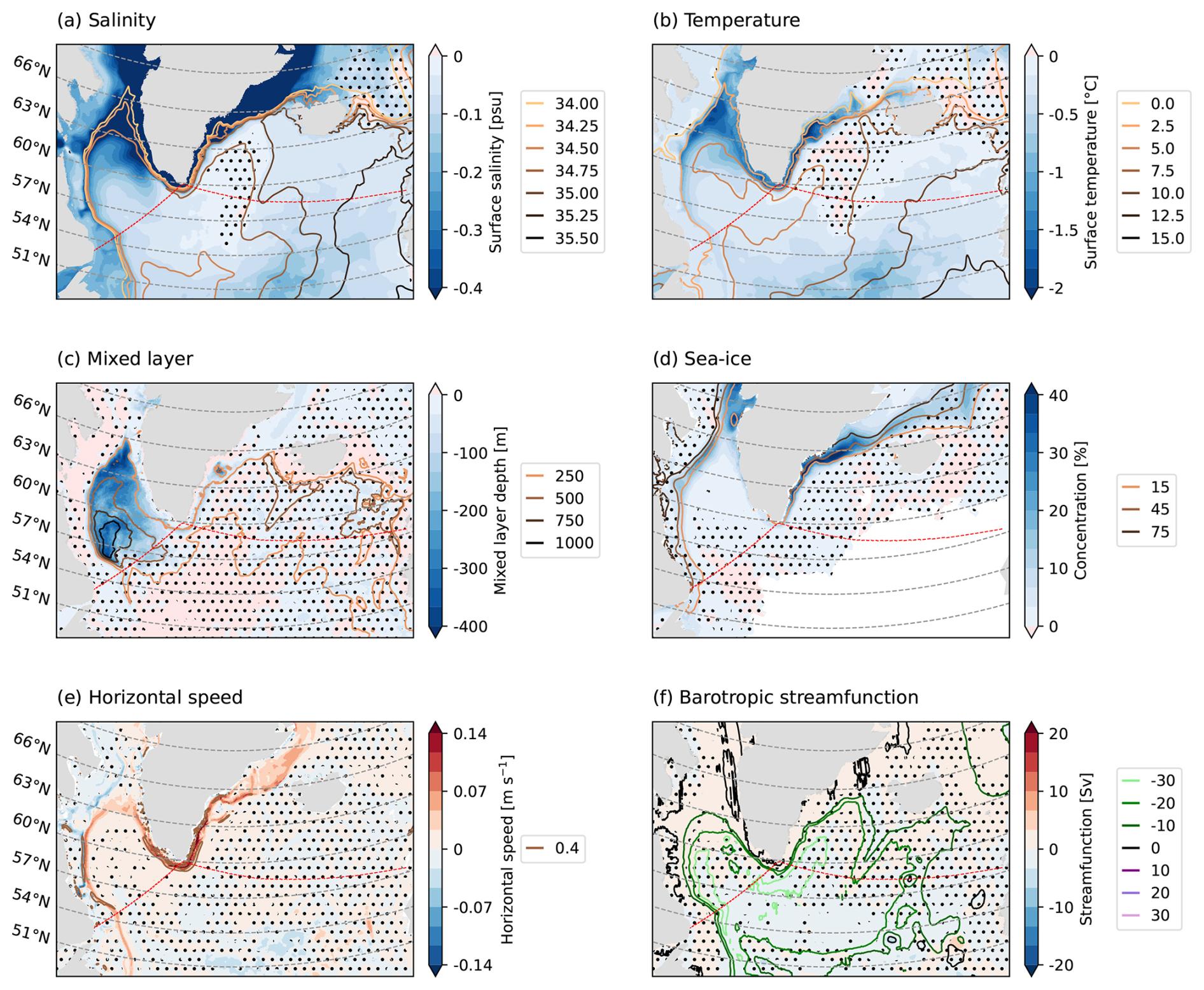
Figure B3 As Fig. 4, showing an enlarged view of the SPNA.

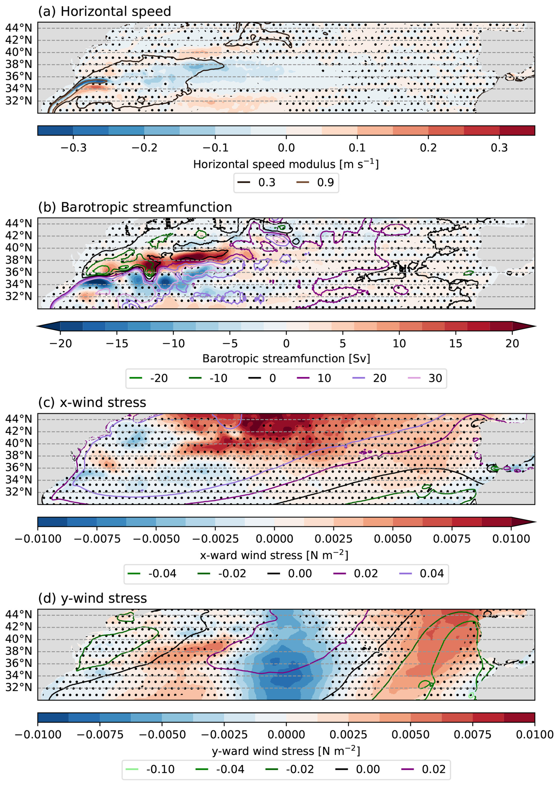
Figure B4 Response to the hosing in the last 10 simulated years for (a) surface horizontal speed modulus, (b) barotropic streamfunction, (c) x-ward wind stress, and (d) y-ward wind stress; filled coloured contours represent the ensemble-mean anomalies of the hosing with respect to the reference control and the contour lines the climatology of the control. Non-significant values as identified by the bootstrap methodology are masked with dots to improve the visibility over the significant areas.

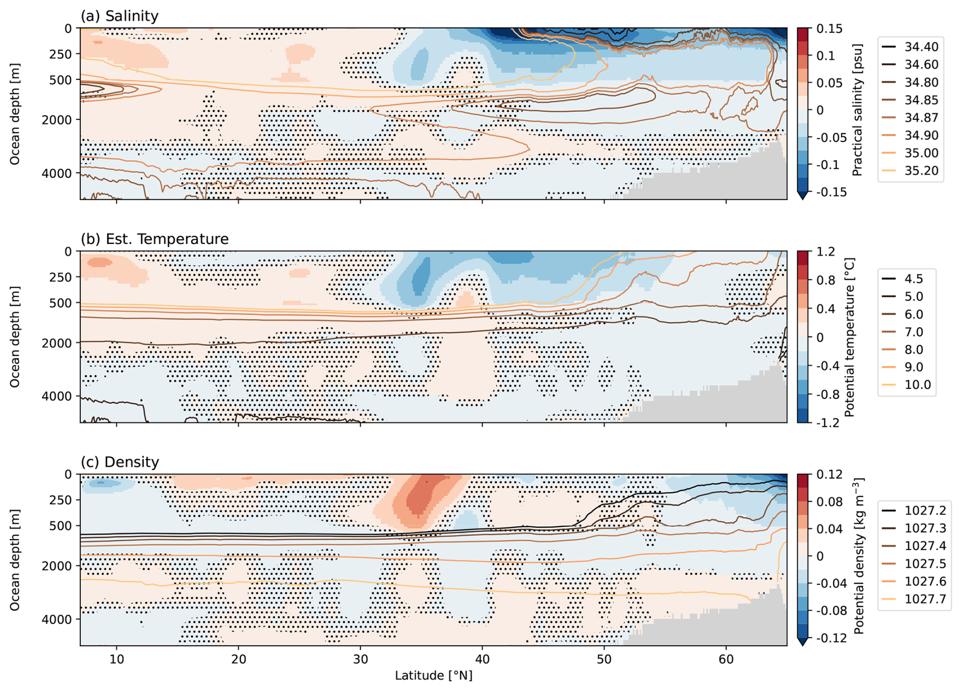
Figure B5 Response to the hosing in the last 10 simulated years for (a) salinity, (b) estimated temperature, and (c) density zonally averaged in the Atlantic basin; filled coloured contours represent the ensemble-mean anomalies of the hosing with respect to the reference control and the contour lines the climatology of the control. Non-significant values as identified by the bootstrap methodology are masked with dots to improve the visibility over the significant areas.

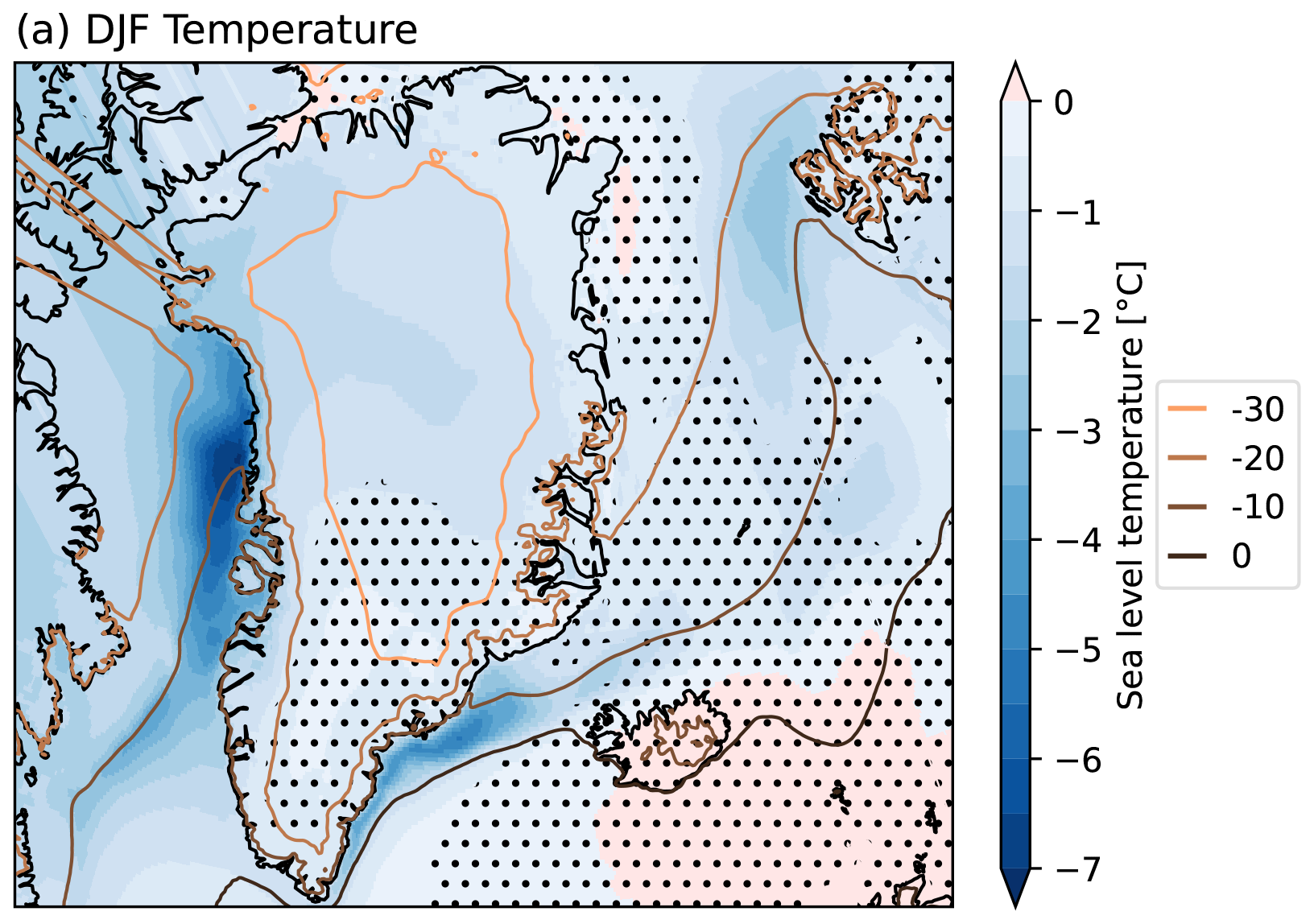
Figure B6 As Fig. 11a, showing an enlarged view around Greenland.