Bottom topography effects on the internal wave climate in the Ionian Sea

The abyssal Ionian Sea is a deep region of interest for the entire ocean circulation of the Mediterranean Sea, since it plays an important role in the ventilation processes of the whole basin. Here we investigate spatial patterns of internal wave climate over the bottom of the Ionian sub-basin. To identify regional features of the internal wave field in terms of vertical shear and strain, we analyze LADCP and CTD profiles, measured across the basin in 2007, covering various seafloor morphologies (shelf, shelf break, and abyssal plain). By introducing broadband statistical quantities derived from the shear–strain variance partition, our results show that increasing seafloor roughness reduces the absolute values of shear-to-strain ratio, a pattern also influenced by correlations between slope and roughness. Roughness appears to constrain waves toward higher frequencies, with high shear-to-strain ratios associated with lower frequencies and flatter propagation angles, and low ratios linked to higher frequencies and steeper beams. Spectral analyses indicate that rougher regions enhance strain variance at small vertical scales while reducing shear variance at larger scales, leading to flatter shear spectra in the low-wavenumber band. Together, these findings suggest that roughness redistributes energy from large-scale (low-mode, low-vertical-wavenumber internal waves with vertical scales O(10²–10³ m)) toward small-scale (high-vertical-wavenumber internal waves with vertical scales O(10–10¹ m)), fundamentally altering the balance of internal wave energy across scales. These results provide useful knowledge for ad hoc finescale parameterization based on seafloor topography.

1 Introduction

The abyssal circulation, when particularly constrained by seabed topography, can bring to the generation of internal waves (IWs) that enhance finescale shear (i.e., vertical variation of the horizontal velocity) and strain (i.e., vertical gradient of isopycnal displacements) over rough bathymetry (Polzin et al., 1997). The resulting small-scale mixing due to breaking of IWs is, therefore, likely responsible for vertical energy transport, which contributes to ocean ventilation (Munk, 1966; Osborne and Burch, 1980; Walin, 1982; Wunsch and Ferrari, 2004; Garrett and Kunze, 2007; Nikurashin and Ferrari, 2013; Ferrari, 2014; Ferrari et al., 2016; Cavaliere et al., 2021; La Forgia et al., 2021).

Despite its thorough implications in the ocean circulation, the relationship between the intensity of overturning circulation and deep, IW-induced mixing rates is not yet fully understood (Garrett and Laurent, 2002; Ferrari, 2014). Paucity of deep ocean measurements hampers our knowledge on abyssal mixing processes and, consequently, ocean heat content variability (Munk and Wunsch, 1998; Ferrari and Wunsch, 2009; Nikurashin and Ferrari, 2011; Waterhouse et al., 2014; de Lavergne et al., 2016; MacKinnon et al., 2017; Ferron et al., 2017; Artale et al., 2018). On the other hand, it is quite established by now that rough bathymetry leads to enhanced IW generation, scattering, and breaking, and thus increased levels of turbulent dissipation (Polzin et al., 1997; Ledwell et al., 2000; St. Laurent and Garrett, 2002; St. Laurent et al., 2012; Ferrari et al., 2016; Mashayek et al., 2017). The analysis of IW-field characteristics from microstructure and fine-structure observations suggests that bottom-generated IWs play a major role in determining the spatial distribution of turbulent dissipation (Sheen et al., 2013; Kunze et al., 2006; Ferron et al., 2014, 2016).

Recent observations indicate that IW field characteristics, shaped by local topography and forcing, show significant variability not only in amplitude but also in frequency composition, affecting the structure and energy distribution of the wave packets and the resulting turbulent mixing (Chinn et al., 2016). In particular, Chinn et al. (2016) explicitly investigates spatial and temporal variability of the shear-to-strain ratio using moored profilers. These authors show that the ratio varies over more than an order of magnitude (≈0.8–10), it is often controlled by either shear or strain variability (site-dependent), and is strongly influenced by local forcing and topography. These considerations inspired us to investigate the potential role of IWs in mixing processes within the eastern part of the Mediterranean basin, where synchronous Lowered Acoustic Doppler Current Profiler (LADCP) and Conductivity, Temperature, Depth (CTD) data were available.

1.1 The regional oceanographic context

The Mediterranean Sea is often considered as a “miniature ocean”, due to its morpho-bathymetric characteristics and its thermohaline cell, where cold and/or salty waters sink during winter at specific regions and, subsequently, spread to intermediate and deep, near-bottom layers (Wüst, 1961; Bergamasco and Malanotte-Rizzoli, 2010; Millot and Taupier-Letage, 2005; Somot et al., 2006; Tsimplis et al., 2006; Schroeder et al., 2016; Artale et al., 2018). Moreover, among the Mediterranean-type climates, i.e., those defined by temperate, wet winters and hot/warm, dry summers over the western edges of five continents, the Mediterranean is the only one in which the atmospheric variability produces an intense deep-water formation (Seager et al., 2019).

Several analyses of the Mediterranean overturning circulation showed that this marginal basin is well ventilated, in comparison to the world ocean (Wüst, 1961; Malanotte-Rizzoli and Hecht, 1988; Pinardi and Masetti, 2000; Theocharis et al., 2002; Artale et al., 2006; Malanotte-Rizzoli et al., 2014; Schneider et al., 2014). Negative hydrological balance and cold-dry winds, blowing during the winter season, make the Mediterranean Sea an extraordinary place of intense ocean water mass transformation (Pinardi and Masetti, 2000), and thus, an ocean laboratory to study the main processes involved in the global ocean circulation.

Surface water from the Atlantic Ocean enters the Mediterranean basin through the Strait of Gibraltar (Fig. 1a), forming a shallow overturning circulation at the upper layer. Flowing eastward, along the African coasts, this Atlantic water increases its salinity and density, then sinking in the Levantine basin in the eastern Mediterranean and forming the Levantine Intermediate Water (LIW). The LIW flows back into the opposite direction, mixing with the surrounding water mass found along its travel back and leaving the Mediterranean Sea through the Strait of Gibraltar, which works as a salt-valve (Artale et al., 2006). Deep water exchanges between the western and the eastern Mediterranean basins occur within the shallow Sicily Channel (Fig. 1a), which makes the deep-water circulation of the two sub-basins rather independent from each other (Sparnocchia et al., 1999; Napolitano et al., 2003; Béranger et al., 2004; Schroeder et al., 2006). In the eastern basin, the Eastern Mediterranean Deep Water (EMDW) is formed, alternately, in separate regions of the Eastern Mediterranean Sea (Fig. 1a), i.e., the southern Adriatic Sea and the Aegean Sea (Gačić et al., 2010). This cold and high salinity winter water, after deep convection, flows into the Ionian Sea (Wüst, 1961; Roether and Schlitzer, 1991; Schlitzer et al., 1991; Roether et al., 1996; Bensi et al., 2013a, b; Bellacicco et al., 2016), i.e., the deepest sub-basin of the Mediterranean Sea, which has a maximum depth close to the mean depth of the global ocean (Fig. 1a). Such a thermohaline circulation is, therefore, characterized by a superposition of intermediate and deep, zonal and meridional overturning cells (Bergamasco and Malanotte-Rizzoli, 2010).

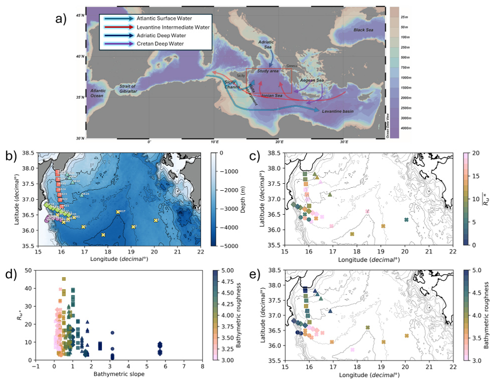
Figure 1 (a) The Mediterranean Sea bathymetry and the main regional features that are discussed within the text; the red box indicates the study area; the panel also shows the main sub-surface circulation pattern of the eastern and central basins; the map was produced in Ocean Data View (Schlitzer, 2018). (b) The Ionian Sea bathymetry and the main regional features that are discussed within the text; LADCP-CTD casts are grouped in five main hydrological transects: four shelf-to-plain transects, i.e., T1 (▴), T2 (▪), T3 (⧫), T4 (•), and one abyssal transect T5 (X). (c) Shear-to-strain ratio $R_{\mathrm{w}}^{\ast }$ at the bottom of the LADCP-CTD profiles, averaged from bins of 80 m in the layer 360–920 m distant from the bottom. (d) Bottom roughness (log10 of var(z)) at the cast sites. (e) $R_{{\mathrm{w}}^{\ast }}$ as a function of bathymetric slope (x-axis), and roughness (in color).

In the Ionian Sea boundary currents show intense downwelling due to their interaction with the topographic constraints while the deepest part of the basin is characterized by extremely weak stratification (Waldman et al., 2018), which induces a deepening and barotropization of the flow (Holte and Straneo, 2017; Send and Testor, 2017). These deep waters are characterized by IW-turbulence and mixing (van Haren and Gostiaux, 2011). Moreover, the Ionian Sea shows a semi-diurnal lunar tidal (M2) and a dominant motion that is around the inertial frequency, mainly as freely propagating IWs (Gerkema and Zimmerman, 2008). For this reason, the Ionian Sea constitutes a unique example for studying the fundamental dynamics and processes of the abyssal layers in the Mediterranean basin, also in the light of turbulent mixing due to IW breaking (Rubino et al., 2012; Artale et al., 2018; Giambenedetti et al., 2024).

1.2 Internal waves and internal tides in the Eastern Mediterranean Sea

Internal waves constitute a fundamental component of the Mediterranean Sea dynamics and play a key role in vertical energy transfer and in the long-term redistribution of heat and tracers. The semi-enclosed geometry of the Mediterranean, its mid-latitude setting, and the presence of steep and irregular bathymetry strongly shape the internal wave field, distinguishing it from that of the open ocean (Millot and Taupier-Letage, 2005; Schroeder et al., 2016).

In particular, the Eastern Mediterranean is characterized by weak deep stratification, quasi-homogeneous abyssal layers, and pronounced topographic gradients, conditions that make this sub-basin highly sensitive to internal wave processes and their variability (van Haren and Gostiaux, 2011). Despite the very low buoyancy frequencies typical of its deep layers, long-term high-resolution temperature measurements revealed intense internal wave activity in the deep Ionian Sea: vertical displacements reached several hundreds of meters, with significant vertical velocities occurring at near-inertial frequencies (van Haren and Gostiaux, 2011). These observations further showed that energetic internal waves advected through abyssal waters can generate strong vertical shear and episodic overturning, indicating that internal wave–induced mixing remains effective even under extremely weak stratification. Weak stratification does not inhibit internal wave dynamics; rather, it modifies their geometry and frequency content, allowing motions with substantial vertical components to develop in the deep basin (van Haren and Millot, 2004, 2005).

Evidence of energetic internal wave variability has also been reported in other Mediterranean sub-basins, such as the Western Mediterranean, where studies in the Tyrrhenian Sea documented active internal wave fields associated with mesoscale circulation and boundary processes (van Haren and Millot, 2004; Buffett et al., 2017). Although these studies focus on different hydrographic and dynamical settings, they support the broader view that internal waves remain dynamically relevant throughout the Mediterranean Sea, including deep environments.

In addition to broadband internal wave activity, recent studies have highlighted the importance of internal tides as a persistent and organized contribution to the Eastern and central Mediterranean internal wave climate. Barotropic tides are relatively weak in the Mediterranean Sea and deep signals are embedded in internal-wave noise (Sannino et al., 2015; van Haren, 2024). However, their interaction with steep bathymetric features, particularly in straits and along major topographic gradients, can generate energetic baroclinic internal tides (Artale et al., 1989; Oddo et al., 2023). Observational and modeling studies in the central Mediterranean have shown that diurnal internal tides, often with Kelvin-like characteristics, are generated at the transition between shallow regions of the Sicily Channel and the deep Ionian basin, propagate away from their generation sites, and contribute significantly to the internal wave energy budget while inducing strong vertical shear (Oddo et al., 2023). Direct observations in the deep Ionian Sea further indicate that baroclinic internal tides penetrate into abyssal layers, modulating temperature and velocity fields even under weak stratification (Giambenedetti et al., 2023).

This body of evidence defines a Mediterranean internal wave climate that is both spatially heterogeneous and dynamically rich, shaped by the interplay between stratification, bathymetry, and tidal forcing. Within this framework, the Ionian Sea emerges as a key region where internal wave activity intersects with large-scale circulation variability. The hydrographic structure of Atlantic Water, Levantine Intermediate Water, and deeper water masses controls internal wave propagation paths and vertical structure (Budillon et al., 2010), while variability in this structure directly affects the efficiency and vertical reach of internal wave–induced mixing, particularly along continental slopes and over irregular bathymetry. On longer timescales, decadal changes in water mass properties further modulate the background conditions for internal wave dynamics and internal redistribution of momentum and tracers (Gačić et al., 2010).

When interacting with rough topography, internal waves and internal tides have been linked to the redistribution of heat and tracers in abyssal layers, contributing to the observed variability of heat content and influencing long-term basin-scale circulation (Artale et al., 2018). This mechanism becomes particularly relevant during periods of reduced deep-water formation, when internal mixing plays an increasingly important role in controlling abyssal ventilation. Internal tides, in particular, represent a continuous source of energy that sustains mixing in deep layers, complementing episodic convective events and reinforcing the coupling between the deep Ionian interior and boundary regions (Giambenedetti et al., 2023; Oddo et al., 2023). Overall, this internal wave climate provides the dynamical background against which internal wave–driven mixing processes operate and contribute to the thermohaline structure and long-term evolution of the Ionian Sea and the broader Eastern Mediterranean basins.

1.3 The KM3NeT project and a preliminary study on seafloor-induced enhancement of isopycnal vertical strain

An intense observational activity was conducted in the Ionian Sea in the framework of the Cubic Kilometre Neutrino Telescope (KM3NeT) project, from April 2006 to May 2009 (Katz, 2006). During the KM3Net cruise (July 2007), hydrographic measurements were spread over a large area, including a section that almost synoptically spanned the central Ionian Sea, from Sicily to Greece. On the western side and up to the central abyssal plane, a marked stratification was found in the deep layers, with a warmer and saltier water on the bottom, below a fresher and slightly colder layer (located approximately at about 2750 m), probably due to deep water formation processes at different times (Sparnocchia et al., 2011). Deep current meter measurements collected in the westernmost part in the period 2007–2008 showed a quite energetic and impulsive abyssal thermohaline circulation pattern, strongly affected by the bathymetric constraints, with maximum velocities up to 15 cm s⁻¹ and cyclonic and anti-cyclonic mesoscale structures, with a period of 5-to-11 d, superimposed on the background geostrophic flow (Rubino et al., 2012; Meccia et al., 2015); these measurements confirmed that tides are “limited” even at depth (i.e., order of ∼ 1 cm s⁻¹).

Artale et al. (2018), by analyzing water column characteristics of the Ionian Sea, observed during the last three decades, focused on the hydrological processes occurring at the bottom layer. They found that the ocean circulation in this abyssal plain is strongly affected by an interplay between advection and diffusion. The progressive warming and salinification of this sub-basin produced warmer near-bottom waters, causing an anomalous heat storage of ∼ 1.6 W m⁻², i.e., a value three times larger than the equivalent climate trend occurring in the same period at global scale (Bindoff et al., 2007). The analysis of Artale et al. (2018) investigated the triggering of a diapycnal mixing due to rough bathymetry. To explore topographic-induced mixing, these authors estimated dissipation rates from the “CTD strain-based” parameterization (Kunze et al., 2006), showing the role of the sea bottom in enhancing isopycnal vertical strain. In particular, they highlighted that the turbulent kinetic energy generated by breaking internal waves is large within a few hundred meters of rough-bottom topography and decays to weaker values farther up in the water column; the bottom enhancement of turbulence reflects the generation of energetic waves, impinging over topography and breaking locally.

From the synergetic use of LADCP and CTD data, collected in the Ionian Sea during the KM3Net cruise in 2007, here we expand the analysis of Artale et al. (2018) to investigate shear variance in addition to strain variance, also exploring the role of topographic characteristics, such as bottom slope and roughness. In particular, our new analysis aims at providing a spatial distribution of shear-to-strain ratio rather than a temporal analysis carried out over a specific region (i.e., the deep area of the Ionian Sea) as in Artale et al. (2018). We explore different seafloor characteristics, in terms of bathymetric gradient and bottom roughness. LADCP profiles, synchronous with CTD casts, allowed estimation of regional values of shear-to-strain ratio R_w (Kunze et al., 2006). In the frame of the Garrett-Munk parametrization (Polzin and Lvov, 2011; See Data and methods), we explore the relation between R_w and topographic features of the Ionian Sea. This approach employs CTD profiles to determine the isopycnal vertical strain ($<{\mathit{\xi }}_z^{\mathrm{2}}{>}_{\mathrm{in}\mathrm{situ}}$), and LADCP profiles for the vertical shear of horizontal velocities ($<V_z^{\mathrm{2}}{>}_{\mathrm{in}\mathrm{situ}}$), assuming that the variance is due to the presence of IWs (see Data and methods). These variances are used to estimate the local energy's level of the IW field, to modulate a canonical value of the dissipation rate of turbulent kinetic energy ε₀ (Garrett and Munk, 1975).

2 Data and methods

2.1 CTD-LADCP casts

Our analysis is based on CTD and LADCP profiles acquired in July 2007 during a research cruise aboard the R/V Urania, conducted within the framework of the KM3NeT project (https://www.km3net.org/ (last access: 22 July 2026); Borghini et al., 2025). CTD-LADCP stations were distributed over a wide area of the northwestern Ionian Sea (Fig. 1a), including strategic sites for the KM3NeT (Neutrino Telescope) infrastructure that had been identified by the particle physics community (Katz, 2006).

CTD data were acquired from the sea surface to the bottom by using a SBE911-plus calibrated before the cruise at the NATO center in La Spezia and were processed by the SBE Sea Soft program, following the standard procedure suggested by the manufacturer. LADCP profiles were collected at a subset of stations using a dual-head system installed on the rosette made of two RDI BB/WH 300 kHz instruments looking upward and downward respectively. The instruments were set to acquire 20 bins with size 10 m and the LADCP data were processed using the LDEO LADCP software Version IX.13 (Visbeck, 2002), using CTD and respective GPS fixes as auxiliary data.

2.2 Finescale parameterization

The small spatial scales (order of centimeters) and intermittent temporal nature (from minutes to hours) involved in internal-wave-driven turbulent mixing, imply that direct measurements are difficult to achieve. Indeed, measurements resolving small-scale turbulence rely on ship-based microstructure profilers, not yet in wide use and, in any case, not on board during the 2007 KM3NeT research cruise. To fill this gap, finescale parameterizations are being used to estimate the turbulent kinetic energy dissipation rate and diapycnal diffusivity from more common instruments, such as CTDs, ADCPs, and Argo profiles (Whalen et al., 2020; Polzin et al., 2014). Finescale parameterizations aim to infer the centimeter-scale turbulent energy dissipation rate, operating on the intermediate [O(10–100) m] vertical wavelengths that are assumed to mediate energy transfer between large and small scales in the ocean (Polzin et al., 2014). Finescale parameterizations are formulated by reference to the Garrett-Munk 75 model (hereafter, GM) (Garrett and Munk, 1975; Cairns and Williams, 1976; Polzin and Lvov, 2011), which provides an empirical expression for the internal wave energy density in the spectral domain. Strain- and shear-based parameterizations allow to estimate the in-situ internal wave energy level, which serves to establish a deviation from the GM model, and to adjust its canonical value for the turbulent dissipation rate ε₀ to a more realistic estimate. In particular, the turbulent dissipation rate can be expressed through the form of the finescale parameterization proposed by Kunze et al. (2006) as:

$$\begin{array}{}\text{(1)}& {\mathit{ϵ}}_{\mathrm{iw}}={\mathit{ϵ}}_{\mathrm{0}}{\displaystyle \frac{N^{\mathrm{2}}}{N_{\mathrm{0}}^{\mathrm{2}}}}{\left({\displaystyle \frac{E}{E_{\mathrm{GM}}}}\right)}^{\mathrm{2}}F\left(R_{\mathrm{w}}\right)L\left(f,N\right)\end{array}$$

where E is the in situ internal wavefield variance and N the in-situ buoyancy frequency, while $E_{\mathrm{GM}},{\mathit{\epsilon }}_{\mathrm{0}}=\mathrm{7}\times {\mathrm{10}}^{-\mathrm{10}}Wk{g}^{-\mathrm{1}}$ and $N_{\mathrm{0}}=\mathrm{5.2}\times {\mathrm{10}}^{-\mathrm{3}}$ rad s⁻¹ are the GM internal wavefield variance, dissipation rate and Brünt-Väisälä frequency, respectively (Garrett and Munk, 1975; Munk, 1981). Depending on whether the parameterization is based on shear or strain, ${\left(E_{\text{in-situ}}/E_{\mathrm{GM}}\right)}^{\mathrm{2}}$ in Eq. (1) can be estimated from the shear variance as $<V_z^{\mathrm{2}}{>}_{\text{in-situ}}^{\mathrm{2}}/<V_z^{\mathrm{2}}{>}_{\mathrm{GM}}^{\mathrm{2}}$, or from the strain variance as $<{\mathit{\xi }}_z^{\mathrm{2}}{>}_{\text{in-situ}}^{\mathrm{2}}/<{\mathit{\xi }}_z^{\mathrm{2}}{>}_{\mathrm{GM}}^{\mathrm{2}}$.

The factor L(f,N) in Eq. (1) represents the latitude effect, calculated as $L(f,N)=f\cos h^{-\mathrm{1}}(N/f)/f_{\mathrm{0}}\cos h^{-\mathrm{1}}(N_{\mathrm{0}}/f_{\mathrm{0}}$) with f the Coriolis parameter and f₀ the Coriolis's frequency at 30°. The term R_w represents the internal wavefield's aspect ratio and the bulk frequency content, and it is defined as the ratio of the buoyancy-normalized shear variance to the strain variance:

$$\begin{array}{}\text{(2)}& R_{\mathrm{w}}=(<V_z^{\mathrm{2}}>/N^{\mathrm{2}})/<{\mathit{\xi }}_z^{\mathrm{2}}>),\end{array}$$

whose effect on dissipation rates ε_iw is modeled by the term F(R_w):

$$\begin{array}{}\text{(3a)}& {\displaystyle }& {\displaystyle }\begin{array}{rl}F\left(R_{\mathrm{w}}\right)=& h_{\mathrm{1}}\left(R_{\mathrm{w}}\right)=\mathrm{3}/\mathrm{4}\left(\mathrm{1}+\mathrm{1}/R_{\mathrm{w}}\right)\sqrt{\mathrm{2}/\left(R_{\mathrm{w}}-\mathrm{1}\right)}\\ & \text{(for shear-based parameterization)}\end{array}\text{(3b)}& {\displaystyle }& {\displaystyle }\begin{array}{rl}F\left(R_{\mathrm{w}}\right)=& h_{\mathrm{2}}\left(R_{\mathrm{w}}\right)=R_{\mathrm{w}}\left(R_{\mathrm{w}}+\mathrm{1}\right)/\left(\mathrm{6}\sqrt{\mathrm{2}{R}_{\mathrm{w}}-\mathrm{1})}\right)\\ & \text{(for strain-based parameterization)}\end{array}\end{array}$$

Equations (3a)–(3b) point out that the error associated with incorrectly assuming R_w is not symmetric (Chinn et al. 2016). For R_w=3 (i.e., the GM value), the correction functions are equal to 1 and do not affect ε_iw. When R_w>3, shear variance dominates, low-frequency internal waves contribute more strongly, and h₁ decreases (thus reducing ε_iw), while h₂ increases (thus increasing ε_iw). When R_w<3, strain variance dominates, high frequency internal waves contribute more to the ratio: h₁ increases (thus increasing ε_iw), h₂ decreases (thus reducing ε_iw). This makes the shear-based parameterizations more effective when R_w>3, and conversely the strain-based parameterizations are more effective when R_w<3 (Chinn et al. 2016).

The determination of R_w requires shear and strain variance measurements through LADCP and CTD observations, respectively. The strain ξ_z is defined as the vertical derivative of the isopycnal displacement and is generally calculated as ${\mathit{\xi }}_z=(N^{\mathrm{2}}-N_{\mathrm{fit}}^{\mathrm{2}})/{\stackrel{\mathrm{‾}}{N}}^{\mathrm{2}}$, where N² is the Brünt-Väisälä frequency, ${\stackrel{\mathrm{‾}}{N}}^{\mathrm{2}}$ a mean value over the vertical segment of water column, and $N_{\mathrm{fit}}^{\mathrm{2}}$ a polynomial quadratic fit: $N^{\mathrm{2}}-N_{\mathrm{fit}}^{\mathrm{2}}$ represents the IW's density perturbation, normalized by ${\stackrel{\mathrm{‾}}{N}}^{\mathrm{2}}$ to obtain the vertical derivative of the isopycnal displacements.

Instead of determining ξ_z, we follow the approach of Ferron et al. (2014) and we determine ξ from the density fluctuations as $\mathit{\xi }=(g/{\mathit{\rho }}_{\mathrm{0}})({\mathit{\rho }}_{\mathrm{HP}}/{\stackrel{\mathrm{‾}}{N}}^{\mathrm{2}}$), with $g/{\mathit{\rho }}_{\mathrm{0}}$ the standard gravity on the reference density, and ρ_HP density filtered by a high-pass Butterworth filter with a cutoff wavelength of 160 m to remove the density fluctuations associated with the background stratification, whose signal would contaminate the integration of the strain spectra (Kunze et al., 2006). This advantageously avoids fitting a polynomial to N² (e.g., quadratic fit in Kunze et al., 2006), that could be inconsistent with the shape of the density profile in case of strong vertical gradients. This method is a variant from Kunze et al. (2006), and follows Ferron et al. (2014). Strain variance is then calculated as the integral of the isopycnal displacement spectra between k_min and k_max:

$$\begin{array}{}\text{(4)}& <{\mathit{\xi }}_z^{\mathrm{2}}>={\int }_{k_{min}}^{k_{max}}{k}^{\mathrm{2}}S\left(\mathit{\xi }\right)\mathrm{d}k.\end{array}$$

Similarly, the shear variance $<V_z^{\mathrm{2}}>$ is obtained from the velocity spectra as

$$\begin{array}{}\text{(5)}& <V_z^{\mathrm{2}}>={\int }_{k_{min}}^{k_{max}}{k}^{\mathrm{2}}S(u,v)\mathrm{d}k.\end{array}$$

To integrate the spectra, k_min and k_max must be carefully determined, as shear and strain rely on different instrument limitations and can be sensitive to distinct phenomenological contributions. In general, k_min is fixed by the choice of the data segment length $k_{min}=\mathrm{2}\mathit{\pi }/L$ rad m⁻¹, where L is generally of 200-to-500 m, i.e., a compromise between the larger vertical wavelengths to be considered (the spectral resolution to be employed) and the desired vertical resolution. For strain, in particular, the integration is performed from $k_{min}=\mathrm{2}\mathit{\pi }/\mathrm{O}(\mathrm{150}$ m) (Kunze et al., 2006; Pollmann et al., 2017; Pollmann, 2020), to exclude contributions from larger-scale background stratification, and continues up to $k_{max}=\mathrm{2}\mathit{\pi }/\mathrm{10}$ m (the GM upper limit).

For shear, a velocity noise is expected to dominate at high wavenumber, especially in weakly stratified layers lacking turbulent microstructures or suspended material (“water-column reflectors”) (Kunze et al., 2006), which tend to reflect the acoustic signal emitted by Doppler profilers like the LADCP. Their absence reduces the quality of the acoustic return, leading to higher measurement uncertainty and potentially spurious velocity variance, especially at small vertical scales. Thus, wavenumbers larger than $k_{max}=\mathrm{2}\mathit{\pi }/\mathrm{O}(\mathrm{100}$–50 m) represent the upper limit range of usable vertical wavenumbers for integration.

An additional saturation criterion is applied to limit the integration of spectra (Gargett, 1990; Kunze et al., 2006). Specifically, the integration is stopped when reaching the saturation value of 0.66N² for the shear variance and 0.22 for strain. This threshold represents the onset of internal wave breaking or turbulence, where the linear internal wave regime breaks down. The corresponding vertical wavenumber k_c at which this value is reached is retained as the upper limit for the integration. This approach constrains the finescale parameterization to physically realistic shear and strain levels, avoiding overestimation of internal wave energy due to instrument noise or unresolved scales, particularly in regions of enhanced energy.

In our case, strain and shear are derived from CTD and LADCP measurements from the bottommost 640 m of each vertical profile. Signals are then linearly detrended and Fourier transformed with a Hamming tapering window. Strain and shear variance estimates are obtained by integrating the 640 m segments, overlapping every 10 m from the bottom to the surface, to account for non-homogeneity in the statistical distribution of the water column properties and to have a statistically robust representation of the fine-scale variability. Final variances are obtained by averaging these overlapping estimates within finite-sized vertical bins (here 80 m), which are independent from the 640 m spectral window length and chosen as a compromise between statistical stability and vertical resolution.

The shear integration upper limit is identified from the LADCP velocity uncertainty. The LDEO LADCP processing (velocity-inversion method; Visbeck, 2002) provides, for each station, a depth-dependent single-bin velocity error profile, i.e. the estimated uncertainty associated with each vertical velocity bin, which is used to constrain the usable shear wavenumber range. The average ${\stackrel{\mathrm{‾}}{V}}_{\mathrm{ERR}}=\mathrm{0.075}$ m s⁻¹ is used to estimate a velocity error by segment as $V_{\mathrm{NOISE}}={\stackrel{\mathrm{‾}}{V}}_{\mathrm{ERR}}/\sqrt{\mathrm{640}\mathrm{m}/\mathrm{10}\mathrm{m}}$. Its associated variance $V_{\mathrm{NOISE}}^{\mathrm{2}}$ is assumed to arise from white velocity noise, uncorrelated in space and therefore uniformly distributed across vertical wavenumbers. In the spectral domain, this corresponds to a flat velocity noise spectrum which, once differentiated, produces a shear noise spectrum used to identify the noise-dominated upper wavenumber limit.

The resulting spectra are then averaged by stratification bins, where we highlight their overall shape and the noise-free bandwidths we retain for integration, from 640 to 107 m (i.e., from 0.01 to 0.06 rad m⁻¹). This choice is conservative, as our lowest stratification levels are close to the $N_{\mathrm{ERR}}=\mathrm{5}\times {\mathrm{10}}^{-\mathrm{4}}$ s⁻¹ (discussed in Kunze et al., 2006), and consistent with the integration set up of Ferron et al. (2014) that stopped the integration at 107 m in the most limitative case. Additionally, this treatment combined both data from downward and upward profiles, in relatively small bin size (10 m), limiting the expected variance loss at short scales due to the various steps of data processing (Polzin et al., 2002; Thurnherr, 2012). For strain, integration is led from 128 to 10 m (i.e., from 0.05 to 0.63 rad m⁻¹; the GM upper limit).

Since shear and strain are integrated on their respective bandwidths, instead of using Eq. (2) directly, the shear-to-strain ratio is calculated as:

$$\begin{array}{}\text{(6)}& \begin{array}{rl}{R}_{\mathrm{w}}^{\ast }=R_{{\mathrm{w}}^{\ast }}^{\mathrm{GM}}& \left(<V_z^{\mathrm{2}}>/<V_z^{\mathrm{2}}{>}_{\mathrm{GM}}\right)/\\ & \left(<{\mathit{\xi }}_z^{\mathrm{2}}>/<{\mathit{\xi }}_z^{\mathrm{2}}{>}_{\mathrm{GM}}\right),\end{array}\end{array}$$

where $R_{{\mathrm{w}}^{\ast }}^{\mathrm{GM}}=\mathrm{3}$, and both shear and strain factors are divided by their corresponding GM values evaluated over the same spectral bandwidths used for each variable. Because $R_{\mathrm{w}}^{\ast }$ in Eq. (6) is derived from variance integrated over finite wavenumber bands, it does not correspond to a single-frequency quantity, but represents a broadband statistical descriptor of the internal-wave shear–strain partition (see Supplement).

2.3 Internal wave beams and impact of bathymetry on R_w

Traditional finescale parameterizations of turbulent kinetic energy dissipation rely on the assumption that the internal wave field follows a GM-like structure. In this framework, a fixed value of the shear-to-strain ratio, typically R_w≈3, is used to represent the relative contributions of vertical shear and isopycnal strain to the finescale energy budget. This fixed value implicitly assumes a broadband, statistically stationary internal wave field, with no significant spatial or temporal variability in spectral composition. However, these models sometimes fail to capture the true dynamics, for instance, near mixing hotspots where the internal wave spectra can be significantly distorted, showing bias toward higher or lower frequencies (Chinn et al., 2016; Polzin et al., 2014; Ferron et al., 2014).

Accumulating evidence from both observations and modeling (Ijichi and Hibiya, 2015, 2017; Takahashi et al., 2021; Dematteis et al., 2024) indicates that this assumption is often violated, especially in regions influenced by complex bathymetry, variable stratification, or energetic boundary currents. In these settings, the internal wave spectrum is distorted, leading to departures from the canonical balance between shear and strain. As a result, R_w can vary significantly in space and time, reflecting changes in the dominant frequency content of the wave field.

Ijichi and Hibiya (2017) used 3D eikonal equations to simulate how internal waves transfer energy across distorted spectra, including variations in the wave energy level, the local buoyancy frequency, and the inertial frequency. Their results confirm that energy transfer rates are consistent with the Henyey et al. (1986) model, which predicts dissipation from internal wave-wave interactions and highlights the importance of the spectral shear-to-strain ratio R_w. The study questions the accuracy of existing finescale parameterization models, particularly in environments with distorted spectra near boundaries or topographic features. To address these limitations, Ijichi and Hibiya (2015, 2017) propose a revised parameterization that explicitly considers both broadband and narrowband spectra. This leads to more accurate dissipation estimates by incorporating a dynamically varying R_w instead of assuming a constant value based on idealized spectral shapes. Their approach was further developed by Takahashi et al. (2021), who showed how vertical wavenumber spectra distortions (such as spectral humps) can bias traditional estimates, emphasizing the need to resolve the spatial variability of R_w.

From a physical point of view, R_w represents the ratio between the buoyancy-normalized vertical shear variance and the isopycnal strain variance. The spectral structure of the internal wave field determines whether energy is primarily stored in the shear (associated with horizontal motion) or in the strain (associated with vertical isopycnal displacement). The theoretical foundation for this lies in the internal wave dispersion relation:

$$\begin{array}{}\text{(7)}& w^{\mathrm{2}}={\displaystyle \frac{N^{\mathrm{2}}{k}_h^{\mathrm{2}}+f^{\mathrm{2}}{k}_z^{\mathrm{2}}}{k_h^{\mathrm{2}}+k_z^{\mathrm{2}}}},\end{array}$$

where w is the wave frequency, $k_h=\left(k_x,k_y\right)$ and k_z the horizontal and vertical wavenumbers, respectively.

Equation (7) shows the intrinsic relation between horizontal (vertical) wavenumber and the shear-to strain ratio. When w≈f, it follows that k_z≫k_h and that the wavefield is dominated by horizontal motion, yielding high shear $\partial u/\partial z$, i.e., the wavefield varies rapidly with depth and more slowly in the horizontal direction. This configuration results in particle motions that are predominantly horizontal but vary significantly over short vertical distances.

In observed internal wave spectra, low-frequency components (near the Coriolis frequency f) tend to concentrate energy in horizontal motions that change rapidly with depth, making shear-dominated fields a hallmark of low-frequency wave regimes (Kunze et al., 2006; Musgrave et al., 2022).

Conversely, when w≈N, k_h≫k_z and the particle motion becomes primarily vertical, enhancing isopycnal displacement and thus the strain $\partial \mathit{\xi }/\partial z$ (i.e., significant vertical displacements of isopycnals). It results that the wave propagates with a nearly vertical beam and the wave field varies slowly with depth. For this condition, although the vertical structure of the wave is broad (i.e., fewer oscillations along z), the amplitude of vertical displacements is large. As a result, the isopycnals experience stronger stretching and compression, leading to enhanced strain energy. This explains why internal waves at high frequencies, despite their low vertical wavenumber, contribute disproportionately to the strain variance. In observed internal wave spectra, higher-frequency components tend to be associated with enhanced isopycnal displacement relative to velocity shear, leading to strain-dominated regimes (Garrett and Munk, 1975; Kunze et al., 2006).

A propagation angle of an internal wave ray can be determined using the dispersion relation:

$$\begin{array}{}\text{(8)}& {\tan }^{\mathrm{2}}\mathit{\alpha }={\displaystyle \frac{N^{\mathrm{2}}-w^{\mathrm{2}}}{w^{\mathrm{2}}-f^{\mathrm{2}}}},\end{array}$$

where ${\tan }^{\mathrm{2}}\mathit{\alpha }=\frac{k_z^{\mathrm{2}}}{k_x^{\mathrm{2}}+k_y^{\mathrm{2}}}$. From Eq. (8), the angle of the wave trajectory (i.e., the beam angle α) relative to the horizontal can be determined. The angle α describes a cone of propagation that supports the wave:

$$\begin{array}{}\text{(9)}& \mathit{\alpha }={\tan }^{-\mathrm{1}}\sqrt{{\displaystyle \frac{N^{\mathrm{2}}-w^{\mathrm{2}}}{w^{\mathrm{2}}-f^{\mathrm{2}}}}}.\end{array}$$

The wave energy propagates with the group velocity c_g, perpendicular to the wave direction k, at an angle $\mathit{\beta }=\mathrm{90}\mathit{°}-\mathit{\alpha }$. For R_w it is possible to derive the following expression (see Kunze et al., 2006; Ijichi and Hibiya, 2015):

$$\begin{array}{}\text{(10)}& R_{\mathrm{w}}={\displaystyle \frac{〈V_z^{\mathrm{2}}〉}{〈{\mathit{\xi }}_z^{\mathrm{2}}〉N^{\mathrm{2}}}}={\displaystyle \frac{w^{\mathrm{2}}+f^{\mathrm{2}}}{w^{\mathrm{2}}-f^{\mathrm{2}}}}\simeq \mathrm{1}+{\displaystyle \frac{\mathrm{2}{f}^{\mathrm{2}}{k}_z^{\mathrm{2}}}{N^{\mathrm{2}}{k}_h^{\mathrm{2}}}}.\end{array}$$

From $R_{\mathrm{w}}^{\ast }$ in Eq. (6) we derive an effective mapped value w^∗ and the associated effective beam slope β^∗, using the classical internal-wave relation only as a geometric mapping. These quantities are not interpreted as the frequency or propagation angle of a single wave, but as broadband statistical diagnostics of the observed shear–strain variance partition. We then compare β^∗ with the local bathymetric slope to organize the observations with respect to bottom geometry.

Equation (9), along with the physical interpretation of Eq. (7), highlights that the wave geometry (i.e., the ratio $k_z^{\mathrm{2}}/k_h^{\mathrm{2}}$) dominates the shear–strain dynamics: for k_z≫k_h we have high shear and R_w values, and for k_h≫k_z high strain values and low R_w. In other words, high R_w values correspond to low-frequency, shear-dominated conditions, while low R_w indicates high-frequency, strain-dominated fields. The dispersion relation is used here as a mapping to define an effective propagation slope, rather than to infer a true wave frequency, following a geometric interpretation of the variance partition rather than a dynamical inference based on monochromatic wave theory. In the general case of a broadband internal wave field, this ratio (i.e., Eq. 10) represents a weighted integral over a distribution of wave components and cannot be reduced to a function of a unique frequency. To avoid confusion with the classical monochromatic internal-wave framework, we therefore introduced the notation $R_{\mathrm{w}}^{\ast }$, w^∗, and β^∗ to denote the broadband statistical quantities derived from the shear–strain variance partition used in this study.

A growing body of evidence shows that turbulent mixing is significantly enhanced in regions of rough bottom topography and sloping boundaries (Polzin et al., 1997; Ledwell et al., 2000; Kunze et al., 2006; Ferrari et al., 2016; Mashayek et al., 2017; Naveira Garabato et al., 2025). Internal wave interactions with these features can lead to reflection, scattering, and energy transfer toward higher vertical wavenumbers, increasing the likelihood of wave breaking and dissipation (Nash et al., 2004; Legg and Adcroft, 2003; Musgrave et al., 2022). In addition to tidal processes, geostrophic flows impinging on small-scale topography generate broadband internal waves that can radiate and dissipate energy locally, contributing to abyssal mixing (Nikurashin and Ferrari, 2010a, 2010b). These mechanisms, collectively, explain much of the spatial variability in observed mixing rates and highlight the importance of accurately representing topographic interactions in ocean mixing parameterizations.

When an internal wave encounters a rough topography, its propagation is disturbed, promoting scattering, reflection, or the generation of higher-frequency waves. This tends to break down low-frequency, large-scale wave structures and shift spectral energy toward higher vertical wavenumbers.

Since strain is associated with large vertical displacements, characteristic of high-frequency waves, this shift leads to a systematic decrease of the shear-to-strain variance ratio R_w in rougher regions, as documented in Kunze et al. (2006), where departures from the canonical Garrett–Munk spectrum were observed in high-roughness environments. As a result, areas of high roughness typically exhibit lower R_w, indicating increased strain. In contrast, smoother topographic regions preserve the lower-frequency shear-dominated character, yielding higher R_w.

In our investigation of the impact of bathymetry on $R_{\mathrm{w}}^{\ast }$ (as a proxy for R_w), we analyze the KM3NeT hydrological stations in relation to bathymetric features such as slope and topographic roughness, calculated using the GEBCO gridded data (https://www.gebco.net, last access: 22 July 2026) over the Ionian Sea area, at 15 arcsec intervals. In particular, slopes are estimated between the hydrological cast position and the points located apart in the eight cardinal directions around, then the average is retained. A distance of 10 km between the two points is chosen to avoid overestimation of the topographic slope, due to the presence of small bathymetric features. Topographic roughness is calculated from the variance of the bathymetry over the same neighboring area (i.e., 20-by-20 km²). $R_{\mathrm{w}}^{\ast }$ values are then compared with the local bathymetric roughness, i.e., the logarithm of the variance of seafloor elevation (Fig. 1c, d).

3 Results

To investigate the influence of bottom topography on internal wave shear-to-strain ratio from Eq. (6), the variance estimates derived from the 640 m sliding windows are subsequently bin-averaged every 80 m from bottom to surface, in order to reduce the variance of individual estimates while preserving vertical structure.

Results show that most of the near-bottom values of $R_{\mathrm{w}}^{\ast }$ are larger than the canonical value of 3, given by the GM model (Fig. 1). Small values, from 1.01 to 10, are generally observed in the shelf break regions, as well as at some deep stations (Fig. 1c), or close to the Malta escarpment (Fig. 1a, b, c). For deep, offshore casts, estimations show large values. High values of shear-to-strain ratio are evident in the western part of the abyssal plain, between 2000 and 3000 m depth, i.e., along the offshore portion of the four cross-shore transects T1, T2, T3, and T4 (Fig. 1b, c). Here, $R_{\mathrm{w}}^{\ast }$ shows values between ∼ 10 and ∼ 30 (Fig. 1c).

In general, regions with higher roughness show lower $R_{\mathrm{w}}^{\ast }$ (Fig. 1d, e), suggesting, for those regions, a shift toward higher-frequency energy and enhanced vertical displacement (i.e., strain). High values of bottom roughness are distributed along the eastern and northern shelf; a smoother bathymetry is recognized in the abyssal plain (Fig. 1e). By plotting $R_{\mathrm{w}}^{\ast }$ against bathymetric slope and roughness (Fig. 1d), we find that although a linear relationship is difficult to establish, an interesting pattern emerges: increased roughness appears to reduce $R_{\mathrm{w}}^{\ast }$. This effect could also be attributed to the bathymetric slope, as slope and roughness are correlated, with steeper zones leading to greater variance in elevation. We hypothesize that this pattern indicates waves being constrained toward higher frequency bands by the roughness.

Indeed, the increasing $R_{\mathrm{w}}^{\ast }$ corresponds to decreasing frequency and flatter beam angles (i.e., more horizontal propagation), while low $R_{\mathrm{w}}^{\ast }$ indicates steeper beams and higher frequencies (Fig. 2a). The grey vertical line and shaded area in Fig. 2a highlight the mean and observed range of $R_{\mathrm{w}}^{\ast }$ in our dataset, contextualizing the frequencies and angles involved. This framework sets the stage for comparing beam angles with local bathymetric slopes. A Δ-slope is inferred as the difference between the beam angle in Eq. (9) and the bathymetry slope. This angle controls the reflection regime: near-critical conditions (Δ-slope ≈0°) are associated with a redistribution of energy toward higher vertical wavenumbers, leading to enhanced vertical shear, while more supercritical conditions favor upward energy propagation and relatively stronger vertical displacements (strain) (Musgrave et al., 2022). $R_{\mathrm{w}}^{\ast }$ is clearly related to Δ-slope (Fig. 2b): higher $R_{\mathrm{w}}^{\ast }$ values correspond to smaller angle differences, while lower $R_{\mathrm{w}}^{\ast }$ values are associated with steeper conditions. This indicates a shift in the bulk structure of the internal wave field, illustrated by the associated w^∗ distribution (Fig. 2c), with frequencies increasing as Δ-slope grows. Additionally, roughness appears to constrain the dynamical range of $R_{\mathrm{w}}^{\ast }$ dispersion. This suggests a critical threshold where high frequencies and smaller scales begin to dominate over shear. Bottom slope and roughness are therefore interpreted here as complementary, but not equivalent, descriptors of the seafloor. Slope primarily describes the large-scale geometric relation between the internal-wave field and the boundary. Roughness, instead, describes smaller-scale bathymetric variability able to scatter the wave field and redistribute variance toward shorter vertical scales. Because both quantities covary in our study region, we do not attempt to isolate their independent causal contributions; rather, we interpret roughness as a modulation of the slope-controlled geometric framework.

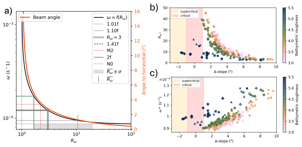
Figure 2 (a) Correspondence between R_w and w (black), and the beam angle associated with R_w (orange), computed at the average latitude of the study (36.75° N). Typical values, from high to low R_w, are reported. The average R_w value of our study is indicated with the vertical line marker, and its distribution range is indicated by the gray area. (b) Distributions of $R_{{\mathrm{w}}^{\ast }}$ and (c) w^∗ in the layer 360–920 m distant from bottom, in function of the difference between the associated beam angle and the bathymetry slope (Δ-slope). Roughness is indicated in color. Higher values on the x-axis indicate a beam angle steeper, relative to the bathymetry slope, while lower values indicate a beam aligning with the slope. The critical range where the alignment is close to be parallel to the slope is arbitrarily marked by the shaded red area from −1 to 1 degrees, out of which a supercritical range is indicated in orange.

By organizing the shear and strain spectra into bins of roughness and Δ-slope to identify whether specific bandwidths are affected, one might expect enhanced signals at larger vertical scales (≈300 m) or smaller scales (≈100 m), depending on the preferential frequency content potentially enhanced by the bathymetric features. The resulting spectra (Fig. 3c) show that strain variance increases at high vertical wavenumbers (small vertical scales) in those regions characterized by the highest roughness (bin 5.1). A tendency toward reduced shear variance at low wavenumbers is observed in rougher regions, accompanied by a flattening of the shear spectrum. Given the limited number of realizations, these differences are interpreted as systematic patterns rather than statistically significant changes. Indeed, shear spectra under rougher conditions (blue spectra in Fig. 3b) appear flatter in the lower wavenumber band compared to smoother regions. Intermediate roughness levels (green spectra in Fig. 3b) show increased energy around vertical scales of 64 m, potentially indicating enhanced energy distribution at shorter scales. Strain spectra exhibit a distinct pattern for the highest roughness, with higher energy levels compared to other bins. These increases in both shear and strain energy levels are statistically robust, as confirmed by a dedicated bootstrap and permutation-based significance analysis (see Supplement), showing coherent variability across configurations and no systematic dependence on bandwidth selection. These observations suggest that increasing roughness reduces energy distribution at larger scales (shear lower band) while enhancing strain variance contributions at smaller scales (upper band). We note that, for this analysis, although wavelengths shorter than 10 m are already excluded, an additional low-pass filtering is applied to prevent the potential inclusion of noise leaking. To isolate the influence of slope geometry, we use the beam-to-slope angle difference Δ-slope. The shear spectra in Fig. 3c shows a clear dependence on Δ-slope. Indeed, higher $R_{{\mathrm{w}}^{\ast }}$ values correspond to smaller angle differences, while lower $R_{{\mathrm{w}}^{\ast }}$ values are associated with steeper conditions. This indicates a shift in frequency content, with frequencies increasing as Δ-slope grows. Spectra in Fig. 3c are coherent with what we observed in Fig. 2 and suggest a critical threshold where high frequencies and smaller scales begin to dominate over shear: the range of $R_{{\mathrm{w}}^{\ast }}$ appears to be limited when the roughness increases. However, we do not have enough data to establish if there exists an actual “threshold value” of roughness above which the spread of $R_{{\mathrm{w}}^{\ast }}$ is limited. This interpretation is further confirmed by the patterns observed in both Figs. 3 and 4: as Δ-slope approaches 0, lower frequencies become dominant, indicating more horizontal motion. This is associated with increased shear and a higher prevalence of critical Richardson instability events (Fig. 4a, b), where the Richardson number is defined as $R_i=\frac{N^{\mathrm{2}}}{\left[{\left(\frac{\partial u}{\partial z}\right)}^{\mathrm{2}}+{\left(\frac{\partial v}{\partial z}\right)}^{\mathrm{2}}\right]}$: R_i values show their minimum values tending toward criticity with low values of delta slope (i.e., flat angles). Yet, the deviation from the GM model is evident in the shear ratio, with values exceeding 8–10 times the model (Fig. 4c, d), while the strain consistently remains below the GM model's predictions (Fig. 4e, f).

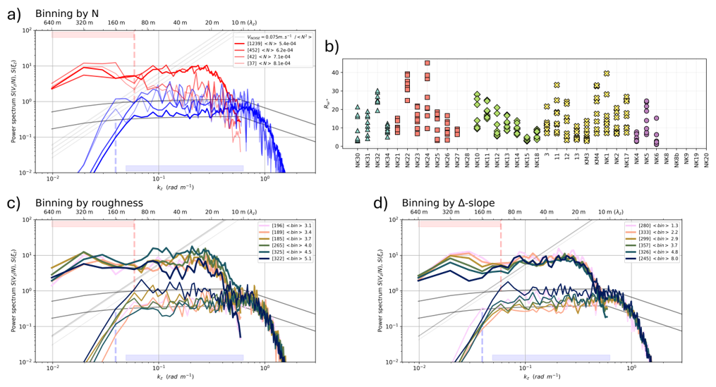
Figure 3 (a) Buoyancy-normalized shear (red) and strain (blue) wavenumber spectra, with their associated GM model (upper black line: shear; lower black line: strain). Spectra are averaged by bins of stratification (thick to thin, from weak to higher stratification). Number of spectra by bins, with the average N of the bin are reported in legend. Shear noise spectra associated with a noise velocity of 0.075 m s⁻¹ are indicated in gray (thickness indicates its association to the N bins). Instrumental wavenumber limits are indicated with the vertical dashed lines: upper limit of $\mathrm{2}\mathit{\pi }/\mathrm{128}$ rad m⁻¹ for shear due to noise contamination; lower limit of $\mathrm{2}\mathit{\pi }/\mathrm{160}$ rad m⁻¹ for strain to filter the large-scale background stratification. Retained wavenumber bandwidths for integration are indicated with the shaded ranges on top and bottom (640–107 m for shear; 128–10 m for strain). Although wavelengths shorter than 10 m are already excluded, an additional low-pass filtering is applied to prevent the potential inclusion of noise leaking. (b) Associated estimates of $R_{{\mathrm{w}}^{\ast }}$ are shown by station and by vertical bins of 80 m, within the same bottom 1000 m layer (lower panel). (c, d) Buoyancy-normalized shear (top) and strain (bottom) wavenumber spectra, with their associated GM model (upper black: shear; lower black: strain). Spectra are averaged by bins of roughness (c), and by bins of the difference between the beam angle and the bathymetry slope angle (d). For both (c) and (d) number of spectra found by bins and the average bin value are reported in legend. Shear noise spectra associated with a noise velocity of 0.075 m s⁻¹ are indicated in gray (thickness indicates its association to the N bins). Instrumental wavenumber limits are indicated with the vertical dotted lines: upper limit of $\mathrm{2}\mathit{\pi }/\mathrm{128}$ rad m⁻¹ for shear due to noise contamination; lower limit of $\mathrm{2}\mathit{\pi }/\mathrm{160}$ rad m⁻¹ for strain to filter the large-scale background stratification. Retained wavenumber bandwidths for integration are indicated with the shaded ranges on top and bottom (640–107 m for shear; 128–10 m for strain).

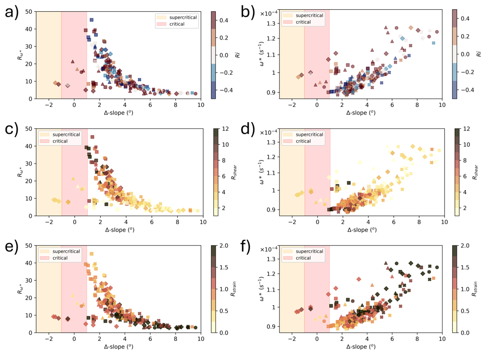
Figure 4 Distributions of $R_{{\mathrm{w}}^{\ast }}$ (left) and w (right) in the layer 360–920 m distant from the bottom, in function of the difference between the associated beam angle and the bathymetry slope angle. Colours are used to indicate (a, b) a bulk Richardson number (in logarithmic scale), (c, d) the shear-to-shear-GM ratio, (e, f) the strain-to-strain-GM ratio. Higher values on the x-axis indicate a beam angle steeper, relative to the bathymetry slope, while lower values indicate a beam aligning with the slope. The critical range where the alignment is close to be parallel to the slope is arbitrarily marked by the shaded red area from −1 to 1°, out of which a supercritical range is indicated in orange.

4 Discussions and conclusions

Our analysis in the Ionian Sea contributes to the investigation of the IW mixing, as described by Kunze et al. (2006). We focused on hydrological stations where we took advantage of synchronous LADCP and CTD profiles from which we infer regional values of the near-bottom ratio between shear and strain variances ($R_{{\mathrm{w}}^{\ast }}$). We note that our definition of $R_{{\mathrm{w}}^{\ast }}$ is meant to give a statistical representation of the classical (single-wave frequency) R_w, usually found in literature (e.g., Kunze et al., 2006; Polzin et al., 2014; Ijichi and Hibiya, 2015, 2017). The finescale parameterization is formally written in terms of the classical shear-to-strain ratio R_w. Here, $R_{{\mathrm{w}}^{\ast }}$ is used only as a broadband, band-limited observational diagnostic of the shear–strain variance partition, allowing us to investigate its spatial variability in relation to bottom topography without interpreting it as an exact monochromatic R_w. Our goal, in particular, was to quantitatively assess the spatial patterns of shear-to-strain ratio to highlight the role of morpho-bathymetric features in enhancing dissipation and diffusion rates, in terms of depth, slope, and roughness.

We found a general relationship between seafloor characteristics and the shear-to-strain variance ratio ($R_{{\mathrm{w}}^{\ast }}$). Smaller Δ-slope values, corresponding to closer alignment between the effective beam slope and the bathymetric slope, are associated with higher $R_{{\mathrm{w}}^{\ast }}$ values and a relatively more shear-dominated internal-wave field. Larger Δ-slope values are associated with lower $R_{{\mathrm{w}}^{\ast }}$ values and a relatively stronger strain contribution. Increasing roughness further organizes these distributions into distinct scatter patterns while reducing the dynamic range of $R_{{\mathrm{w}}^{\ast }}$, suggesting a roughness-induced redistribution of energy toward strain-dominated smaller vertical scales. This interpretation is supported by the spectra, which show enhanced small-scale strain variance and a tendency toward reduced large-scale shear variance over rougher topography, although individual spectral bands remain noisy. This, in turn, supports the hypothesis that gentler slopes and smoother seafloor generate lower-frequency internal waves, whereas steeper and rougher topography favors higher-frequency waves, leading to a corresponding increase in the shear (strain) contribution. In particular, for the northwest group of stations (i.e., the shelf-to-plain transects T1, T2, and T3; Fig. 1b), we found coherent trends of $R_{{\mathrm{w}}^{\ast }}$, which co-varies with depth, slope, and roughness.

Our observations suggest that, in rougher conditions, internal wave energy is redistributed toward smaller vertical scales (higher vertical wavenumbers), leading to an enhancement of strain variance relative to shear. The resulting decrease in $R_{{\mathrm{w}}^{\ast }}$ indicates a wave field that departs from shear-dominated regimes and becomes increasingly strain-dominated, consistent with enhanced spectral distortion over rough topography (Chinn et al., 2016). In abyssal waters (i.e., deeper than 3000 m), specific stations of transects T4 and T5 (e.g., from Station NK6 to Station 11; Fig. 1b) show a behavior similar to the one observed in the shelf-to-plain transects: $R_{{\mathrm{w}}^{\ast }}$ increases with distance from the shelf break, starting from $R_{{\mathrm{w}}^{\ast }}$ ∼ 10, although we are in abyssal waters. We notice, however, that those abyssal stations of Transect 4 that show low values of $R_{{\mathrm{w}}^{\ast }}$ (i.e., values we expect in rough areas) are close to the topographic constraints of the Malta Escarpment (Fig. 1a), where energetic mesoscale meandering features and vortical structures at the bottom, were observed (Rubino et al., 2012; Meccia et al., 2015). These low values of shear-to-strain ratio may be due to the eventual mesoscale eddy–internal wave coupling that could represent a sink of eddy energy and then a source of IW energy (Polzin, 2010; Takahashi et al., 2021). These abyssal stations in Transect 4 may therefore represent those particular, “nontraditional” cases (Gerkema and Shrira, 2005) where deep mesoscale activity is able to trigger diapycnal mixing by breaking of IWs. Finally, we notice that in Ferron et al. (2014) a 160 m-high-pass filter is explicitly applied on density to remove largescale density variations, that can lead to spectral shape differing from Kunze et al. (2006) for scale larger than 160 m. The overall level of our strain spectra is also closer to GM, which is consistent with the fact that our observed internal-wave field is close to GM in amplitude.

Kunze et al. (2006) suggested that the lack of reflectors in the water column at deep locations could lead to an overestimation of the shear variance, reflected ultimately in strong values of R_w. However, within the limits of our analysis, the shear spectra do not display clear indications of dominant noise contamination, given the conservative choices adopted for the integration bands.

In addition to this potential instrumental bias, we also examined whether thermohaline structure could affect the interpretation of $R_{{\mathrm{w}}^{\ast }}$. In particular, we observe that the bottom layer of several eastern abyssal stations exhibits thermohaline gradients that could be consistent with double-diffusive regimes (Miles, 1961; Ruddick, 1983; Thorpe, 2005). However, an additional analysis of Turner angles (Tu) indicates that only a few thin layers fall within active values $\left|\mathrm{Tu}\right|\mathit{>}\mathrm{75}$° (13.6 % for salt Fingering, 1.8 % for diffusive convection). These few layers do not display particularly significant density structures. We therefore consider that double-diffusive layers are only minimally represented in our dataset and are unlikely to significantly influence the overall analysis of $R_{{\mathrm{w}}^{\ast }}$.

Our analysis on shear-to-strain ratio is based on CTD-LADCP casts that were carried out during a single oceanographic cruise in 2007. Therefore, we cannot perform any analysis on the temporal variability of the spatial patterns we observe. However, we can frame our results within the interannual analysis (1977–2011) presented by Artale et al. (2018). These authors highlighted the presence of a “new” bottom Ionian water, from the 2003, resulting from the continuous entrainment of the warmer, upper waters, a process that would cause a loss of kinetic energy and gain of potential energy in the deep layer (Marotzke and Scott, 1999). Based on this analysis we can argue that the spatial pattern of shear-to-strain ratio we observe is likely depicting the particular barotropization of the bottom layer found in Artale et al. (2018), characterized by a homogeneous bottom layer between 3000 and 4000 m depth and weak horizontal gradients of potential temperature over the Ionian basin (Artale et al., 2018). Our results are consistent with previous studies (i.e., Chinn et al., 2016; Polzin et al., 2014; Ferron et al., 2014) in showing that shear–strain balance is not universal but systematically modulated by environmental conditions, here specifically seafloor roughness and slope in the Ionian Sea.

Finally, our analysis aims to provide useful insights for ocean circulation models, which are often too sensitive to vertical eddy diffusivity and are largely affected by inaccuracy at deep layers (Gargett and Holloway, 1992; Wright and Stocker, 1992). In particular, the large variability of the shear-to-strain ratio we found, may help deriving both dissipation rate of turbulent kinetic energy and diapycnal diffusivity in the finescale parameterization.