Linking large-scale climate modes to local wave climate and storm surge: insights from a weather typing approach

Understanding temporal variations in nearshore sea states is crucial, as they affect shoreline evolution and coastal hazard potential. Local sea state conditions are influenced by large-scale climate modes, yet the underlying mechanisms remain not fully understood. Previous studies have mainly established the climate–sea state links through correlation analyses or other statistical methods. This study investigates whether weather typing, a statistical downscaling method, can provide a physically interpretable link between climate modes and local wave and storm surge variability. The analysis was conducted at Hartlepool, UK, where 36 weather types were previously developed to assess the exposure to coastal hazards for a local nuclear power station. Six climate indices were examined, and we found that the North Atlantic Oscillation (NAO) and the Scandinavian pattern (SCAND) have significant correlations with local wave and storm surge variables. The analysis reveals that, in response to the phases of NAO or SCAND, storm surge distributions exhibit changes in the mean and standard deviation, peak wave period distributions shift between bimodal and near-unimodal shapes, and wind waves and swell show different dominant directions. Using weather types, these response patterns can be traced back to synoptic circulation conditions characterized by different prevailing winds, spatial patterns of storm activity, and local atmospheric pressure. NAO and SCAND modify the occurrence probabilities of these synoptic conditions, thereby providing a probabilistic link between large-scale climate modes and local sea states. This research demonstrates the potential of weather types to offer new perspectives on the impact of climate modes on local sea states.

1 Introduction

Large-scale climate modes are periodic variations in the Earth's climate system that occur over timescales ranging from years to decades. One notable example is the North Atlantic Oscillation (NAO), the leading mode of climate variability in the Euro-Atlantic region, which involves the redistribution of atmospheric mass between the Arctic and the subtropical Atlantic (Hurrell et al., 2003). Alongside NAO, the East Atlantic pattern (EA), the Scandinavian pattern (SCAND), and the Western Europe Pressure Anomaly (WEPA) are also identified as significant modes of climate variability in this region. It has long been recognized that shifts between phases of these climate modes can bring profound changes to surface temperature, precipitation, wind patterns, and other meteorological properties (Lamb and Peppler, 1987; Hurrell, 1995; Hurrell et al., 2003). More recently, studies have increasingly focused on their broader impacts beyond the climate system. Significant correlations have been identified with oceanographic variables including wave climate (e.g. Martínez-Asensio et al., 2016; Odériz et al., 2020; Scott et al., 2021) and water level/storm surge (e.g. Wakelin et al., 2003; Woodworth et al., 2007; Chafik et al., 2017). Moreover, the influence on sea state conditions has been further linked to shoreline variability (e.g. Wiggins et al., 2020; Masselink et al., 2023), flood exposure (e.g. Muis et al., 2018; Arcodia et al., 2024), and coastal vulnerability (e.g. Barnard et al., 2015).

Research into the impacts of climate modes has significant implications. A deeper understanding of how coastal environments respond to climate modes will enable the use of climate projections to identify areas vulnerable to coastal flooding and erosion driven by climate change, supporting coastal management and adaptation strategies (Barnard et al., 2015; Wiggins et al., 2020). By establishing more robust relationships between large-scale climate modes and local-scale environmental drivers, there is also the potential to utilize climate indices for improved reproduction of sea state conditions and better forecasting of coastal change. Hilton et al. (2020) demonstrated that a shoreline prediction model achieved increased accuracy when its synthetic wave generation algorithm was informed by prior knowledge of the NAO and WEPA indices. In other studies, climate indices were incorporated as predictors to represent interannual or intra-seasonal climate variability in stochastic emulators of water levels (Anderson et al., 2019) and wave climate (Cagigal et al., 2020). In addition, understanding these relationships allows for the investigation of historical coastal evolution using reconstructions of climate indices over centennial timescales, offering valuable insights into long-term coastal variability (Wiggins et al., 2020).

Numerous studies have established links between climate modes and sea state variability by analysing the temporal correlation between climate indices and specific sea state parameters, such as significant wave height and extreme sea level (e.g. Semedo et al., 2015; Morales-Márquez et al., 2020; Scott et al., 2021; Freitas et al., 2022). These relationships are usually displayed in 2D maps to reflect the spatial patterns and to identify places with robust links, often supplemented by regression coefficients as a measure of the sensitivity of sea state variability to climate indices (e.g. Wakelin et al., 2003; Woodworth et al., 2007; Hochet et al., 2021). Regression analysis has also been employed to evaluate combinations of indices in situations where a singular index fails to fully explain observed variance (e.g. Frederikse and Gerkema, 2018; Scott et al., 2021), thereby providing insights into the relative contribution from each index (Frederikse and Gerkema, 2018). More complicated statistical techniques, including Empirical Orthogonal Function, Canonical Correlation Analysis, and Redundancy Analysis, have also been applied to associate patterns of variations between atmospheric circulation and sea state parameters (e.g. Wang and Swail, 2001; Woolf et al., 2002; Chafik et al., 2017; Hochet et al., 2021).

Meanwhile, climate variability is also widely investigated through weather regimes (e.g. Hurrell et al., 2003; Cassou et al., 2004; Pohl and Fauchereau, 2012), which are recurrent (occur repeatedly), persistent (last for multiple days, e.g. 10 d), and quasi-stationary (large-scale motion is stationary in the statistical sense) atmospheric circulation patterns (Michelangeli et al., 1995). The underlying idea is that the continuously evolving weather system can be represented by a finite set of weather regimes, often obtained by clustering techniques. This concept enables the analysis of atmospheric circulation dynamics across different timescales by examining the temporal distribution of these regimes.

Beyond understanding climate dynamics, the concept of weather regimes has also influenced downscaling studies, where a similar but distinct approach, often referred to as weather typing, is used to link localized atmospheric or oceanographic information with synoptic-scale weather conditions (Wilby and Wigley, 1997). A key distinction lies in the number of patterns used: downscaling typically requires a larger set (around 30–100) to capture subtle variations in atmospheric circulation and improve the estimation of local variables, whereas studies of low-frequency climate variability focus on broader-scale features and can be effectively represented by fewer patterns (usually no more than 8 Michelangeli et al., 1995). Consequently, weather types (WTs) tend to have shorter durations and more frequent transitions, which may not fully align with the definition of a weather regime. Nevertheless, previous work showed that weather types could be associated with certain climate modes (e.g. Camus et al., 2014; Neal et al., 2016), highlighting their potential to connect the variability of large-scale climate circulation and local sea states.

While direct correlation analyses can identify whether climate indices are associated with wave or surge variability, they provide limited information on the synoptic-scale atmospheric conditions through which these associations develop. In this research, we use weather types as an intermediate layer linking interannual climate modes to daily-scale atmospheric circulation and, ultimately, to local sea state variability. The method's ability to characterize detailed, local multivariate sea state conditions while tracing back the synoptic conditions responsible for them can potentially offer new insights into the role of climate modes in affecting regional hydrodynamics. This work has three objectives: (1) identify the climate modes contributing to the sea state variability at the selected location; (2) characterize the responses of storm surge and wave climate under different phases of the identified climate modes; and (3) identify the atmospheric processes linking climate modes to the corresponding sea state responses based on weather types.

2 Data and method

This study is part of a broader project assessing coastal hazard exposure at UK nuclear power stations using a hybrid statistical-dynamical downscaling approach. We applied the weather typing method at the Hartlepool nuclear power station, which is located on the north-east coast of England (Fig. 1). A set of 36 WTs was developed to characterize the regional synoptic circulation patterns, which were then linked to the wave and storm surge conditions at an offshore location near the nuclear station. This research expands upon our previous work (Zhong et al., 2025) by incorporating large-scale climate modes into the weather type analysis.

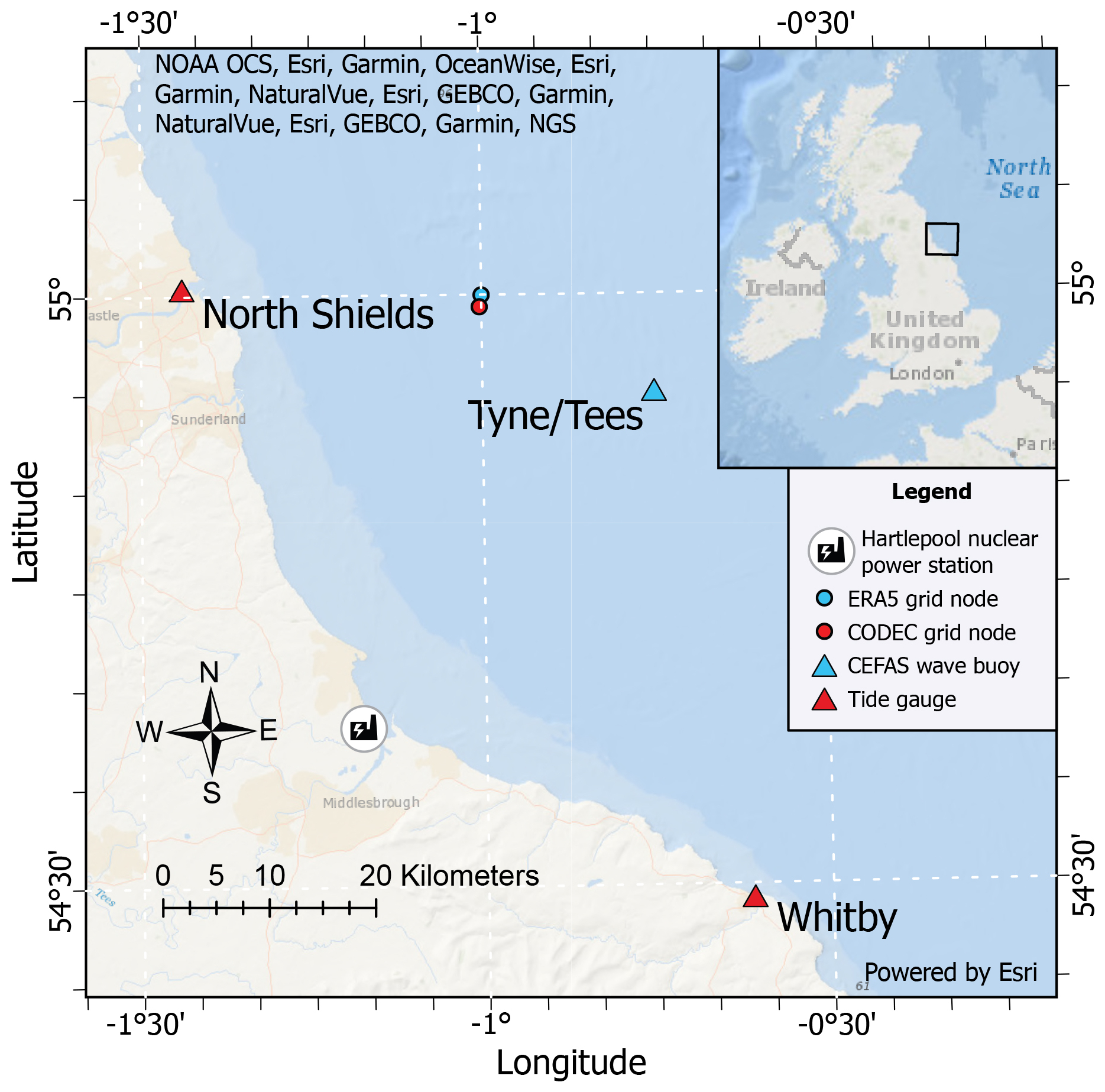
Figure 1 Locations of the nuclear station and data sources (modified from Zhong et al., 2025).

2.1 Weather typing

The weather typing method was originally developed in Camus et al. (2014) and later applied and validated in Hartlepool by Zhong et al. (2025). This statistical downscaling approach is designed to establish empirical relationships between larger-scale atmospheric conditions (predictors) and local multivariate oceanographic variables (predictands). Given a statistically robust link between the predictors and predictands, weather typing can serve as an efficient alternative to dynamical downscaling (i.e. process-based dynamical modeling) while maintaining good accuracy. This section provides a brief introduction to weather typing, outlining the datasets involved and the main procedures.

Three types of data were used to derive the WTs. Large-scale atmospheric conditions were represented by sea level pressure (SLP) from ERA5, the fifth-generation global atmospheric reanalysis produced by the European Centre for Medium-Range Weather Forecasts (ECMWF) (Hersbach et al., 2020). The local wave climate conditions were also obtained from ERA5 at an offshore grid node near Hartlepool (55° N, 1° W; see Fig. 1). The wave node is around 24 km away from the coast and at a depth of 74 m. The wave climate conditions included hourly variables characterizing both the combined wind waves and swell (including significant wave height H_s, mean wave period T_m, peak wave period T_p, and mean wave direction θ_m) as well as individual wind wave and swell components (including significant height $H_s^w$ and $H_s^s$, mean period $T_m^w$ and $T_m^s$, and mean direction ${\mathit{\theta }}_m^w$ and ${\mathit{\theta }}_m^s$, where the superscripts ^w and ^s denote wind wave and swell components, respectively). Storm surge (SS) conditions at a neighbouring location were obtained from CODEC (Muis et al., 2020), a global dataset for extreme sea levels and storm surges driven by wind and atmospheric pressure from ERA5. Validation of wave and storm surge was conducted in Zhong et al. (2025). In summary, H_s showed good agreement between ERA5 and the CEFAS wave buoy, whereas T_p displayed some discrepancies. SS from CODEC also compared well with those derived from tide gauges, although CODEC tends to slightly underestimate high surge values and overestimate low surge values. Consequently, a bias correction method was applied to SS. The weather typing analysis was conducted using data from 1979 to 2018.

The first step involved defining the atmospheric predictors in terms of variable selection, spatial domain, and temporal coverage. Here, the predictors were constructed from daily mean SLP and the squared SLP gradient (SLPG, which is closely related to the geostrophic winds) fields over a spatial domain extending from 26 to 76° N and 40° W to 30° E, with a 2° spatial resolution. The predictors were averaged over 4 d to reflect the time scale typical for extratropical storms in the North Atlantic basin (Gulev et al., 2001; Haigh et al., 2016), which are the main drivers of wave climate and sea level variability in this region. To facilitate the classification of WTs, a Principal Component Analysis (PCA) was performed to reduce the dimensionality of the predictors while preserving 95 % of the data variance.

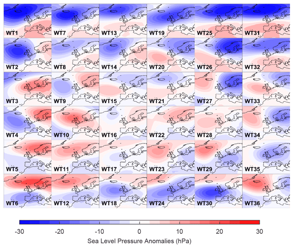
Next, a regression-guided classification (Camus et al., 2016) was implemented to categorize the predictors into a group of representative synoptic circulation patterns (i.e. weather types). This consisted of two key steps. First, a multivariate linear regression model was fitted between the predictors and a group of selected predictands (daily means of H_s, T_p, θ_m, and daily maximum storm surge). The estimates from the regression model captured the synoptic-scale influence on the local sea states while filtering out irrelevant signals. Second, a semi-supervised clustering was performed on a dataset composed of the predictors and the estimated predictands from the regression model, with a weighting parameter introduced to control the relative contributions of the two components. The k-means clustering was then implemented to partition the dataset into 36 clusters, minimizing the total variance within a cluster. The cluster centroids were subsequently projected back into the original high-dimensional space and plotted in a 6-by-6 lattice, where clusters with lower centroid distances (i.e. higher similarity) are positioned closer together. Figure 2 displays the circulation patterns for 36 WTs, represented by the anomalies of SLP, as climate variability is typically analysed in terms of deviations from the climatology (Hurrell et al., 2003).

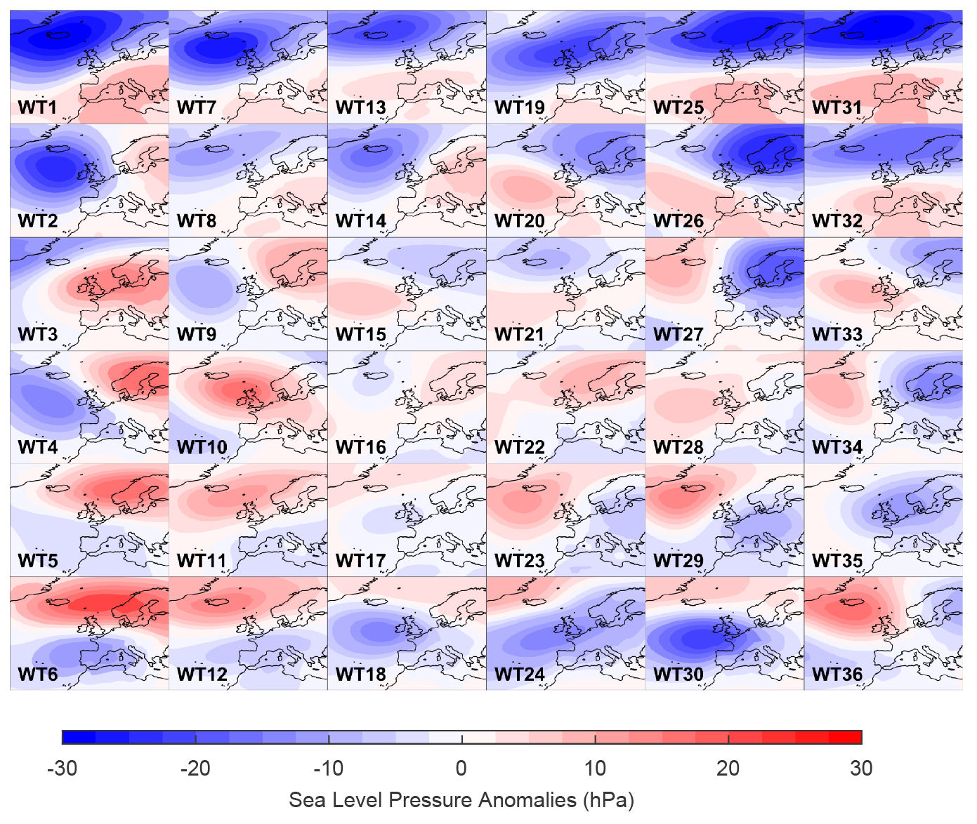
Figure 2 The synoptic circulation pattern of 36 WTs. SLP anomalies are derived using the 1979–2018 mean as the reference baseline.

Once the WTs were defined, the relationships between predictors and predictands were established by collecting the predictands recorded on all dates when a specific WT occurred. This allowed for the derivation of empirical distributions of wave and storm surge variables associated with each WT. Model validation confirmed the effectiveness of WTs and their empirical relationships in providing estimates of multivariate sea state variables with generally good accuracy, as well as their limitations in reproducing wave direction and extreme wave events (Zhong et al., 2025).

Sensitivity analysis was conducted to investigate the impact of different model configurations on the performance of sea state downscaling. The analysis considered factors such as the choice of predictor variables, the spatial domain of the model, the number of days over which the predictors were averaged, the spatial resolution of the predictors, the number of WTs, and the weighting parameter used in the semi-supervised clustering. Some of the main findings are as follows: (1) using both SLP and SLPG as predictors outperforms using either one individually; (2) model performance shows low sensitivity to the spatial domain; (3) increasing the spatial resolution of the predictors does not significantly improve model performance; (4) increasing the number of WTs improves model performance, but more WTs means the associated sea state distributions for each individual WT are less representative. A detailed discussion was provided in Zhong et al. (2025).

2.2 Climate indices and their correlation with local sea state variability

The behaviour of climate modes is widely studied through climate indices, which are numerical representations of the phase and intensity of atmospheric or oceanic variability patterns. In this study, we examined six key climate indices: NAO, EA, SCAND, Arctic Oscillation (AO), East Atlantic Western Russian pattern (EA/WR), and WEPA. These are the main modes of climate variability over the North Atlantic and European regions and have been commonly considered in previous research (e.g. Martínez-Asensio et al., 2016; Hochet et al., 2021; Scott et al., 2021).

The first five indices were obtained from the National Oceanic and Atmospheric Administration (NOAA) Climate Prediction Center. They were calculated using Rotated Principal Component Analysis (Barnston and Livezey, 1987), applied to monthly mean standardized 500 mb height anomalies in the Northern Hemisphere (20–90° N). The WEPA index, available at Scott et al. (2020), was developed in Castelle et al. (2017) to explain the variability of winter wave activity along the Atlantic coast of Europe. Its definition is based on the normalized SLP difference between the stations Valentia (Ireland) and Santa Cruz de Tenerife (Canary Islands).

A correlation analysis was conducted using these six climate indices to identify climate modes relevant to wave climate and storm surge variability at Hartlepool. The analysis focuses on the extended winter months (December to March, DJFM), which aligns with previous research (e.g. Martínez-Asensio et al., 2016; Scott et al., 2021). This is the period when the atmospheric pressure in the Northern Hemisphere exhibits the greatest variability and perturbations reach their largest amplitudes, significantly influencing local wind fields, wave climate, and sea levels (Hurrell et al., 2003; Shimura et al., 2013). By contrast, during summer, when westerlies and extratropical storms are weaker, mesoscale processes become more relevant in determining local wave characteristics, particularly in coastal areas (Semedo et al., 2015).

First, we calculated the mean climate indices, the mean wave variables (including the combined wind waves and swell as well as individual wind wave and swell components), the 99th percentile of H_s (H_s99), and the 1st, 50th, and 99th percentiles of SS (SS₁, SS₅₀, and SS₉₉) in each DJFM period. Next, Kendall's τ coefficient was calculated to measure the correlation for scalar quantities (i.e. storm surge, wave height, and wave period). We selected this measure of correlation because it does not require variables to be normally distributed (which is the assumption for the Pearson correlation) and is less sensitive to outliers than Spearman's ρ. For circular variables (wave direction), we used a circular–linear correlation method described in Berens (2009). The correlation coefficient ρ_cl between a linear variable x and a circular variable θ is defined as:

$$\begin{array}{}\text{(1)}& {\displaystyle }{\displaystyle }{\mathit{\rho }}_{cl}=\sqrt{{\displaystyle \frac{{\mathit{\rho }}_{cx}^{\mathrm{2}}+{\mathit{\rho }}_{sx}^{\mathrm{2}}-\mathrm{2}{\mathit{\rho }}_{cx}{\mathit{\rho }}_{sx}{\mathit{\rho }}_{sc}}{\mathrm{1}-{\mathit{\rho }}_{sc}^{\mathrm{2}}}}},\end{array}$$

where ${\mathit{\rho }}_{sx}=\text{corr}(\sin \mathit{\theta },x)$, ${\mathit{\rho }}_{cx}=\text{corr}(\cos \mathit{\theta },x)$, ${\mathit{\rho }}_{sc}=\text{corr}(\sin \mathit{\theta },\cos \mathit{\theta })$, and corr() denotes the Pearson correlation coefficient. The range of ρ_cl is between 0–1, with greater values indicating stronger association between x and θ.

2.3 Associating WTs with climate modes

The synoptic circulation patterns of certain WTs have similar structures to some climate modes. For example, WT31 is characterized by strong negative pressure anomalies over Iceland and the Norwegian Sea and positive pressure anomalies across mid-latitudes (Fig. 2). This pattern closely resembles the spatial structure of the positive phase of NAO, which indicates a potential link. However, not all WTs have distinct spatial patterns, and some WTs may reflect the influence of multiple overlapping climate modes.

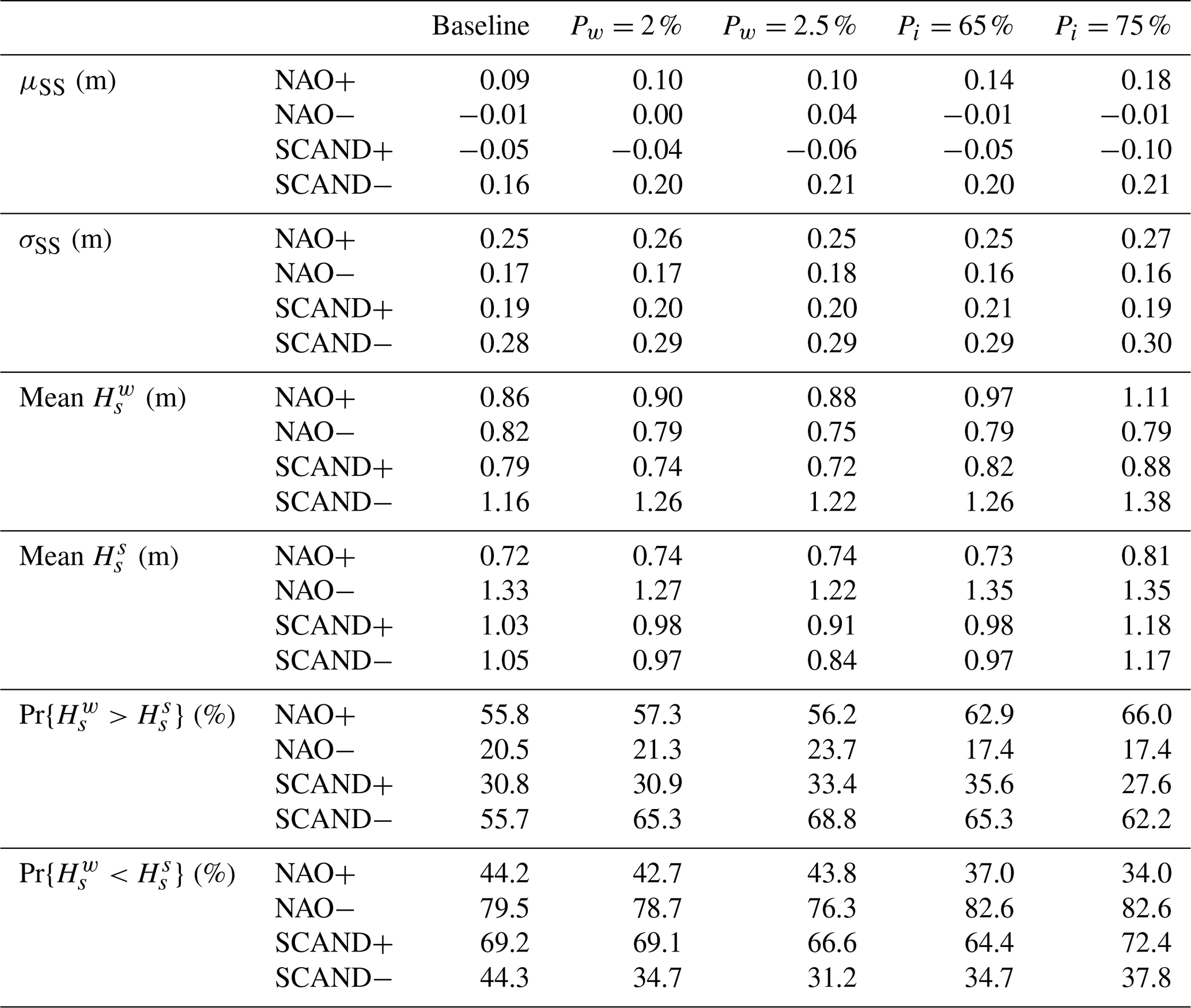
To establish a more general and robust link between WTs and climate modes, we calculated the percentage of WT occurrence under a positive or negative climate index phase during DJFM. A WT was associated with a specific index phase if its occurrence probability under that phase exceeded a threshold (P_i), which was set to 60 %. For instance, WT1 was classified under positive NAO because 89 % of its occurrence coincided with a positive NAO index, compared to just 11 % with a negative index. The occurrence percentage naturally served as an indicator of the strength of this association. The selection of this threshold was subjective, and the choice of 60 % was intentionally conservative to ensure that each climate index phase was associated with a larger set of WTs. Additionally, WTs with a low occurrence frequency during DJFM (P_w) were excluded from the categorization to maintain statistical robustness in the association. We used a threshold of 1.5 % for P_w. The results are listed in Table B1 and visualized in Fig. 3. A sensitivity analysis was conducted on the values of P_i (i.e. 60 %, 65 %, 70 %) and P_w (i.e. 1.5 %, 2 %, 2.5 %) to examine the robustness of this approach. It should be noted that the association between WTs and climate modes is probabilistic rather than deterministic. In other words, WTs associated with a given climate index phase tend to occur more frequently during that phase, but they can also occur during the opposite phase, albeit at lower probabilities.

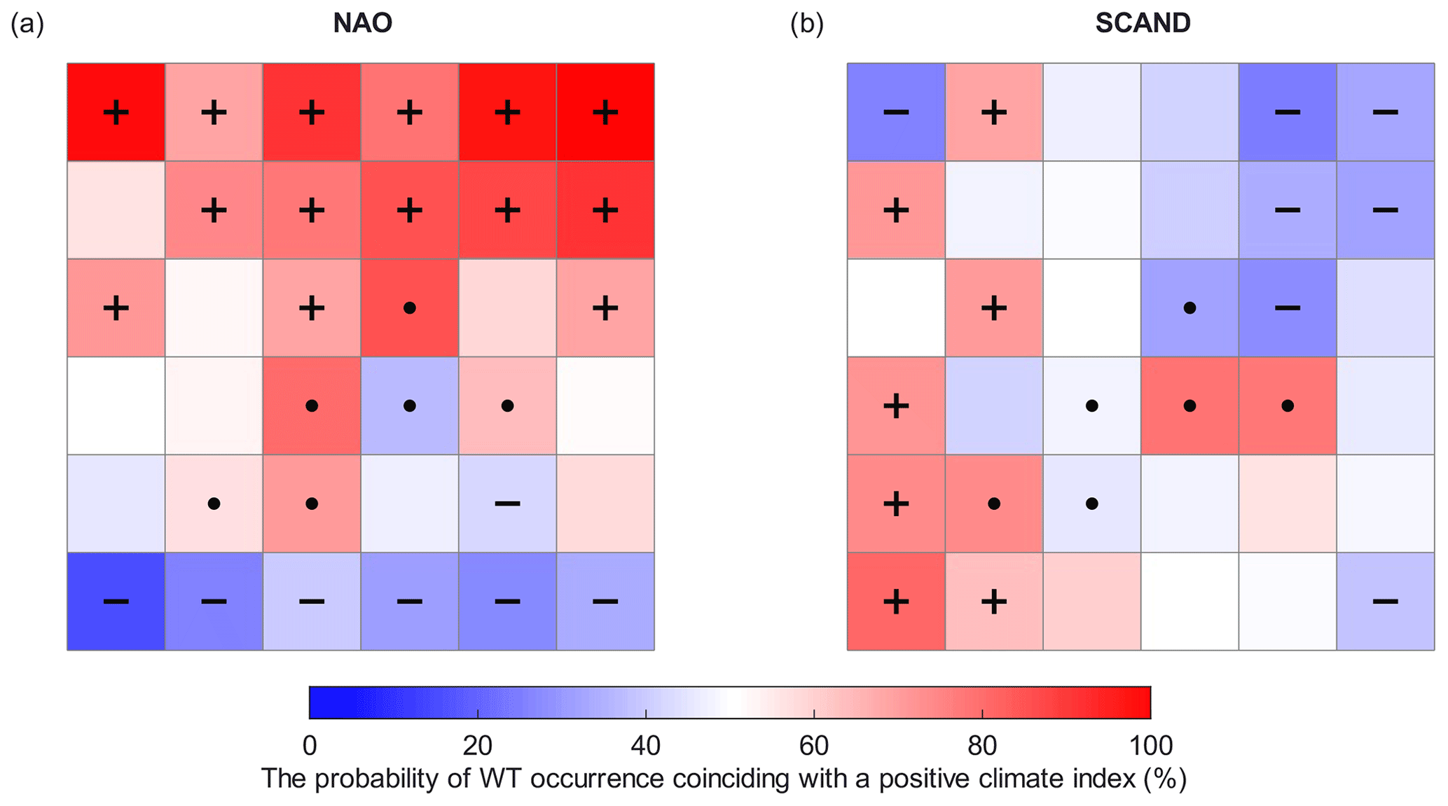
Figure 3 Percentage of WT occurrence coinciding with a positive climate index during DJFM. Each cell in the 6×6 lattice corresponds to the WT of the same location in Fig. 2. WTs are marked with a plus sign (+) if classified in the positive phase, a minus sign (−) if in the negative phase, or a dot if excluded from the classification due to low occurrence frequency during DJFM (based on the P_w threshold).

2.4 Parametrization of atmospheric processes

Climate modes influence sea states by modifying atmospheric circulation, such as wind and storm patterns. To understand the role these individual processes play in the connection between climate modes and sea state variability, we parametrized their effects on wave climate and storm surge. For each atmospheric process, we identified the key parameters that represent its intensity and related them to sea state conditions. It should be noted that the explicit physical mechanisms underlying air–sea interactions are complex and beyond the scope of this research.

The wave climate is dependent on the effects of local wind and distant storms. Gulev and Grigorieva (2006) performed a Canonical Correlation Analysis over the North Atlantic and North Pacific and found that wind wave variability is closely linked to local wind speed, whereas swell is more strongly associated with the frequency of deep (<980 hPa) cyclones. To parametrize the impact of local wind, we obtained the surface wind speed W from ERA5 using the eastward and northward 10 m wind components (U and V, respectively). The wind speed was averaged over a 0.5°×0.5° grid box centred on the study location to represent regional wind conditions. For the impact of extratropical storms on waves, we used the storm track dataset derived in Camus et al. (2024). The dataset was generated by applying a storm tracking algorithm to sea level pressure and 10 m wind speed fields at 0.25° resolution from ERA5. The algorithm calculated the vortex strength based on the U and V wind components and identified potentially significant storms by applying both a vortex strength threshold (0.5) and a sea level pressure threshold (1010 hPa) on an hourly basis. Once a storm was detected, it was tracked over consecutive time steps using a nearest neighbour detection approach within a maximum distance of 5°. The storm frequency was parametrized by the number of hours with storms detected in each 1°×1° grid box divided by the total number of hours.

Storm surges are mainly driven by changes in the atmospheric pressure and the force of wind stress (Pugh and Woodworth, 2014). The impact of atmospheric pressure is commonly known as the inverse barometer effect, which is expressed as:

$$\begin{array}{}\text{(2)}& {\displaystyle }{\displaystyle }\mathrm{\Delta }\mathit{\eta }=-\mathrm{\Delta }{P}_A/\mathit{\rho }g,\end{array}$$

where Δη is the change in sea level, ΔP_A is the local pressure anomaly relative to the global mean sea level pressure over the entire ocean (assumed to be constant at 1013.3 hPa in most applications), ρ is water density, and g is the gravitational acceleration (Pugh and Woodworth, 2014). Hence, the impact of atmospheric pressure on storm surge was parametrized by ΔP_A. Since each WT is represented by a spatial pattern of SLP, the ΔP_A at our study location (55° N, 1° W) was estimated by SLP values on the four nearest grid points. These values were averaged with a weight of the cosine of the corresponding latitude to account for the convergence of meridians at higher latitudes. Storm surge generated by wind occurs through the shear stress exerted by wind on the sea surface, which pushes water toward certain directions. In shallow waters, the storm surge caused by wind stress can be expressed in the following form:

$$\begin{array}{}\text{(3)}& {\displaystyle }{\displaystyle \frac{\partial \mathit{\eta }}{\partial x}}={\displaystyle \frac{{\mathit{\rho }}_{\text{air}}{C}_d{W}^{\mathrm{2}}}{\mathit{\rho }gD}},\end{array}$$

where $\frac{\partial \mathit{\eta }}{\partial x}$ is the gradient of sea level, ρ_air is air density, C_d is the drag coefficient (related to wind speed due to increasing roughness of sea surface with a stronger wind), W is wind speed, and D is water depth (Pugh and Woodworth, 2014). Since our focus is on representing the effect of wind stress on storm surge rather than quantifying wind-generated surge itself, we parametrized this effect using W only.

3 Results

3.1 Correlations between climate indices and local sea states

The first objective of the study is to identify climate modes contributing to the sea state variability at Hartlepool. This was achieved through a correlation analysis between six climate indices and local wave and storm surge variables, with the results given in Table 1. Significant correlations (at the 95 % confidence level) are found for NAO, AO, SCAND, and WEPA, with moderate to strong associations. NAO and AO show similar correlation patterns, particularly for storm surge and wave directions. This is not surprising considering the strong correlation between these two indices, with a Pearson coefficient of 0.80 between their winter means. Indeed, there has been ongoing debate about whether they represent distinct phenomena or different manifestations of the same underlying climate variability (e.g. Ambaum et al., 2001; Itoh, 2008). SCAND seems to have the opposite correlation compared to NAO. No significant correlation is found for either EA or EA/WR.

Table 1 Correlation coefficients between winter sea state parameters and winter mean index values. Kendall's τ coefficient was used for wave height, wave period, and storm surge variables, while a circular–linear correlation (Berens, 2009) was calculated for circular variables (θ_m, ${\mathit{\theta }}_m^w$, and ${\mathit{\theta }}_m^s$). Bold values indicate statistical significance (p-value<0.05). The analysis was conducted for the period 1979–2018.

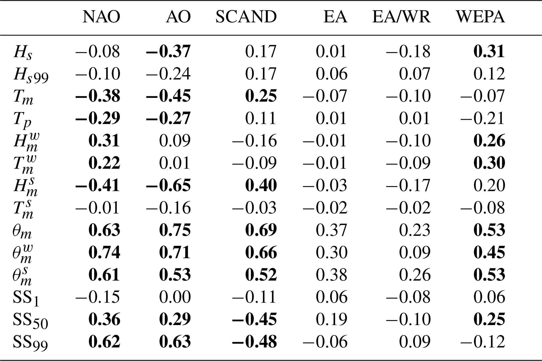
Although four indices were identified as relevant to local sea state variability, we focus on NAO and SCAND for further analysis based on the following considerations. The subtle differences between NAO and AO are unlikely to be distinguished by our WTs which only account for the Atlantic region. NAO is chosen as it has been extensively examined in previous studies and may provide a more physically meaningful interpretation of climate dynamics than AO (Ambaum et al., 2001). WEPA is not considered because it is more relevant in regions south of 52° N (Castelle et al., 2017, 2018; Scott et al., 2021).

3.2 The response of sea states to climate indices

The second objective of the study is to characterize the response patterns of wave and storm surge to the selected climate indices. The 36 WTs, along with their empirical distributions of wave climate and storm surge, were associated with the positive or negative phases of NAO (NAO+, NAO−) and SCAND (SCAND+, SCAND−) indices. The categorization of each WT is shown in Fig. 3. WTs that occur more frequently during NAO+ and NAO− are found at the top and bottom of the lattice, while those that occur more frequently during SCAND+ and SCAND− are mainly positioned on the left and right sides, respectively. It should be noted that the positioning of each WT is purely based on the centroid distances (i.e. similarity of their spatial patterns) between its neighbouring WTs and does not consider which climate index phases they are associated with. The reason that most WTs associated with the same index phase are placed together is that they share more or less the same broad-scale atmospheric circulation structure. This section focuses on identifying common response patterns linked to the same index phase and comparing the differences between the positive and negative phases.

3.2.1 Wave climate

The response of wave climate is complicated due to its multivariate nature. For the combined wind waves and swell, the distributions of H_s do not show significant differences between climate index phases (Fig. A1). In contrast, more distinct patterns emerge in T_p. For WTs occurring more frequently during NAO+ (Fig. 4a), the individual T_p distributions typically take two forms: a unimodal distribution with a high peak around 4–6 s and a long tail to the right, or a bimodal distribution with peaks at 4–6 and 10–12 s. As a result, the overall T_p distribution for all WTs that occur more frequently during NAO+ is bimodal, with the left peak being more pronounced than the right. In contrast, WTs with higher occurrence probabilities during NAO− do not exhibit two distinct modes in the overall T_p distribution, which is closer to a unimodal distribution with a broad peak spanning across 5–10 s (Fig. 4b). The pattern observed for SCAND− closely resembles that of NAO+, while the distributions related to SCAND+ are also similar to those seen for NAO− (Fig. 4c and d). These patterns are not observed in the T_m distributions (Fig. A2).

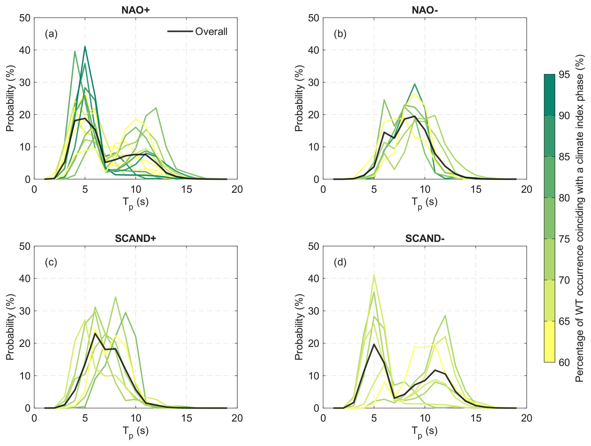
Figure 4 The empirical distributions of hourly T_p associated with WTs that occur more frequently during each climate index phase. Each coloured distribution is associated with an individual WT, with the colour representing the percentage of WT occurrence in particular NAO or SCAND phases in Table B1, thus indicating the strength of the association. The overall distributions (black) are derived from all hourly T_p values from WTs assigned to the same category of climate index phase.

The two modes in T_p likely correspond to wind waves and swell, respectively. These components display different patterns in mean direction and significant wave height in response to NAO/SCAND (Figs. 5, 6, and A3), whereas their mean periods show less pronounced differences between index phases (Fig. A4). For WTs more commonly observed during NAO+, the overall ${\mathit{\theta }}_m^w$ distribution primarily spans between south and west, with the individual distributions for each WT also generally falling within the same range (Fig. 5a). These south-westerly wind waves have similar wave height distributions, with most measuring less than 1 m (Fig. 6a). Swell waves, on the other hand, are primarily from two distinct directions: north and south-east. The northerly waves are observed with higher frequency and larger magnitudes (Figs. 5e and 6e). For WTs that occur more often during NAO−, the overall ${\mathit{\theta }}_m^w$ distribution essentially flips to the opposite side compared to the positive phase, spanning from north to east and somewhat extending into the south (Fig. 5b). The individual ${\mathit{\theta }}_m^w$ distributions exhibit more variability than those of NAO+. Unlike ${\mathit{\theta }}_m^w$, ${\mathit{\theta }}_m^s$ shows more consistency among WTs, with the overall distribution displaying two peaks between north and east (Fig. 5f). For wave heights related to NAO−, swell waves are generally larger than wind waves. In fact, most of these swell waves are also larger than those related to NAO+ (Fig. A3 and Table B2).

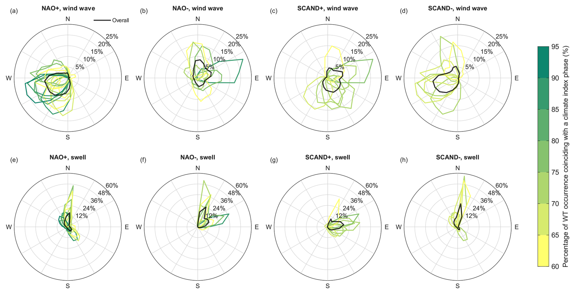
Figure 5 The empirical distributions of hourly ${\mathit{\theta }}_m^w$ and ${\mathit{\theta }}_m^s$ associated with WTs that occur more frequently during each climate index phase (similar to Fig. 4). The radial axis indicates the percentage of wave travelling from each 15° directional bin.

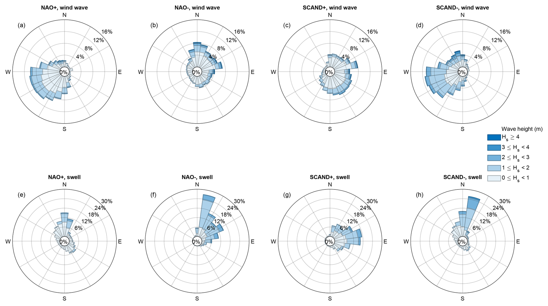
Figure 6 The wave rose diagrams for wind waves and swell associated with WTs that occur more frequently during each climate index phase. Each diagram represents the overall wave distribution of all WTs associated with the same index phase. In addition to directional distribution (as in Fig. 5), the diagrams also show the wave height distribution (indicated by the colour) in each 15° directional bin. The diagrams were generated using the toolbox by Pereira (2026).

For WTs observed more frequently during SCAND+, the overall ${\mathit{\theta }}_m^w$ distribution mainly extends from north to south, covering the eastern half of the wave rose (Fig. 5c). These wind waves are relatively small in height, averaging only 0.79 m (Table B2). In comparison, swell waves are more concentrated in the east and have greater wave heights (Figs. 5g, 6g, and A3). Regarding WTs with higher occurrence probabilities during SCAND−, we also observe a flip in the overall ${\mathit{\theta }}_m^w$ distribution (Fig. 5d) compared to that of SCAND+. Wind waves now dominate the western half of the wave rose, with the majority of them coming from the south-west. Meanwhile, most swell waves travel from a much narrower range in the north (Fig. 5h). In this case, $H_s^w$ and $H_s^s$ are more comparable, with a mean of 1.16 and 1.05 m, respectively (Table B2).

Table B2 also shows the probability of $H_s^w$ being higher or lower than $H_s^s$. Since wave energy is proportional to the square of wave height, this also indicates the likelihood of wind waves or swell dominating the wave energy spectra. Under WTs with higher occurrence probabilities during NAO+/SCAND−, wind wave dominance is slightly more frequent than swell dominance. Conversely, for NAO−/SCAND+, the wave field is more likely to be dominated by swell.

3.2.2 Storm surge

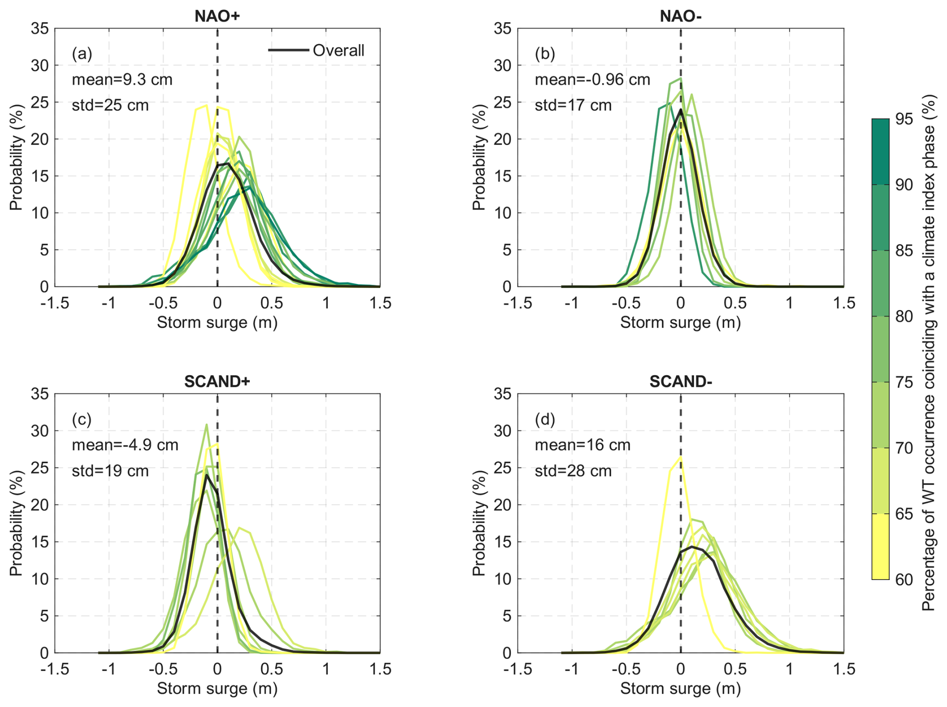
Storm surge distributions for individual WTs typically resemble a normal distribution, but their characteristics (e.g. relative position and spread) vary significantly depending on their association with NAO or SCAND index phases. For WTs with higher occurrence probabilities during NAO+ (Fig. 7a), most distributions tend to shift toward more positive values, meaning that there is a higher proportion of positive surges compared to negative ones. This positive shift is more pronounced for WTs with a higher occurrence percentage when the NAO index is positive (i.e. WTs more strongly associated with NAO+). In addition, WTs with a stronger association tend to have lower and wider peaks, indicating a greater spread in storm surge values. In contrast, for NAO− (Fig. 7b), the distributions generally have a high and narrow peak centred around 0 m. These characteristics can be parametrized by the mean (μ_SS) and standard deviation (σ_SS): the overall storm surge distribution associated with NAO+ has both a higher μ_SS and a greater σ_SS than that of NAO−. Similar patterns are also observed regarding the response to SCAND. The surge distributions related to SCAND− (Fig. 7c) tend to shift to the positive side (positive μ_SS) and have lower and broader peaks (higher σ_SS) compared to WTs occurring more often during SCAND+ (Fig. 7d). It is worth noting that, although some WTs deviate from the general pattern observed within their group, their association with the corresponding index phase is relatively weaker.

Figure 7 The empirical distributions of hourly storm surge values associated with WTs that occur more frequently during each climate index phase (similar to Fig. 4). The means and standard deviations of the overall distributions are provided.

3.2.3 Sensitivity analysis

The response patterns identified previously may be sensitive to the choice of thresholds (P_w and P_i) applied in linking WTs to climate index phases. Hence, we performed a sensitivity analysis to assess how they influence the relationships between key characteristics of sea state conditions and climate modes (Table B3). Despite the variations in statistics, the following patterns remain consistent across all tested cases: (1) mean $H_s^w$ is higher under SCAND+ than SCAND−; (2) mean $H_s^s$ is higher in NAO− than NAO+, but it remains more or less at 1 m in both phases of SCAND; (3) the wave energy spectra are more frequently dominated by wind waves during NAO+/SCAND− and by swell during NAO−/SCAND+; (4) both μ_SS and σ_SS related to NAO+/SCAND− are higher than those linked to NAO−/SCAND+. It is worth noting that as the statistical association between WTs and climate index phases strengthens (i.e. higher P_w or P_i), $H_s^w$ shows an increasing difference between the two phases of NAO (from 0.04 to 0.13 or 0.32 m, respectively).

Moreover, the sensitivity of wave direction to P_w and P_i was tested (Figs. A5 and A6). Overall, the distribution of wave direction is insensitive to these two thresholds, with the exception of the NAO− category, which exhibits noticeable variation as P_w increases.

3.3 Processes contributing to variabilities of wave climate and storm surge

The third objective of this study is to investigate the atmospheric processes linking climate modes to the corresponding sea state responses. At this stage, WTs become particularly relevant, as they provide an intermediate, physically interpretable layer for identifying the synoptic-scale atmospheric conditions through which climate modes influence local sea-state variability. These conditions are examined in terms of wind forcing, storm activity, and atmospheric pressure anomalies.

3.3.1 Wave climate

First, the link between wind forcing and wind waves is examined. We derived the wind pattern associated with WTs that occur more frequently under each climate index phase (Fig. 8). WTs with higher occurrence probabilities during NAO+/SCAND− are characterized by predominantly south-westerly local winds, which is consistent with the corresponding ${\mathit{\theta }}_m^w$ distributions (Fig. 6). In contrast, WTs occurring more frequently during NAO−/SCAND+ exhibit a broader range of wind directions, which still aligns well with the wind wave patterns. Apart from direction, the mean local wind speed W is very well correlated with the corresponding mean $H_s^w$ for each WT, irrespective of index phases, with a correlation coefficient of 0.95.

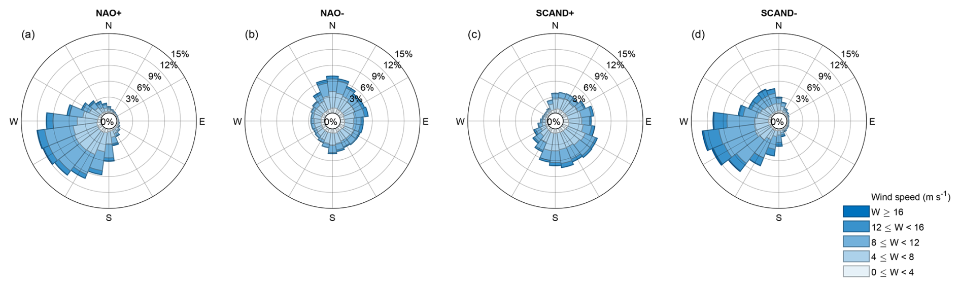
Figure 8 Wind rose diagrams associated with WTs that occur more frequently during each climate index phase, showing the distribution of wind directions (indicating where the wind blows from, consistent with the definition of wave direction) and corresponding wind speeds, similar to Fig. 6. Wind conditions are represented by the regional weighted mean over a 0.5°×0.5° grid box centred on the study location. The diagrams were generated using the toolbox by Pereira (2026).

Next, we explored the possibility of relating swell wave variability to extratropical storm activity. Figure 9 illustrates the spatial distribution of storm occurrence frequency associated with WTs occurring more frequently at different climate index phases. We only focus on the region where swell waves can propagate to our study site, which was estimated by assuming that deep water waves propagate along great circle paths (Pérez et al., 2014). Areas where these paths to the study site are clearly blocked by land were excluded. The resulting source region covers the North Sea and much of the Norwegian Sea. During NAO+/SCAND−, the Norwegian Sea experiences more frequent storms than the North Sea. This pattern is consistent with the corresponding swell wave conditions, where waves predominantly come from the north with higher wave heights. During NAO−, the storm activity shifts toward the North Sea and the southeastern Norwegian Sea. This pattern corresponds with swell waves propagating from more easterly directions. The storm frequency in SCAND+ is lower than the other three cases, but the regions with relatively higher density (the southern North Sea) generally align with the dominant swell direction.

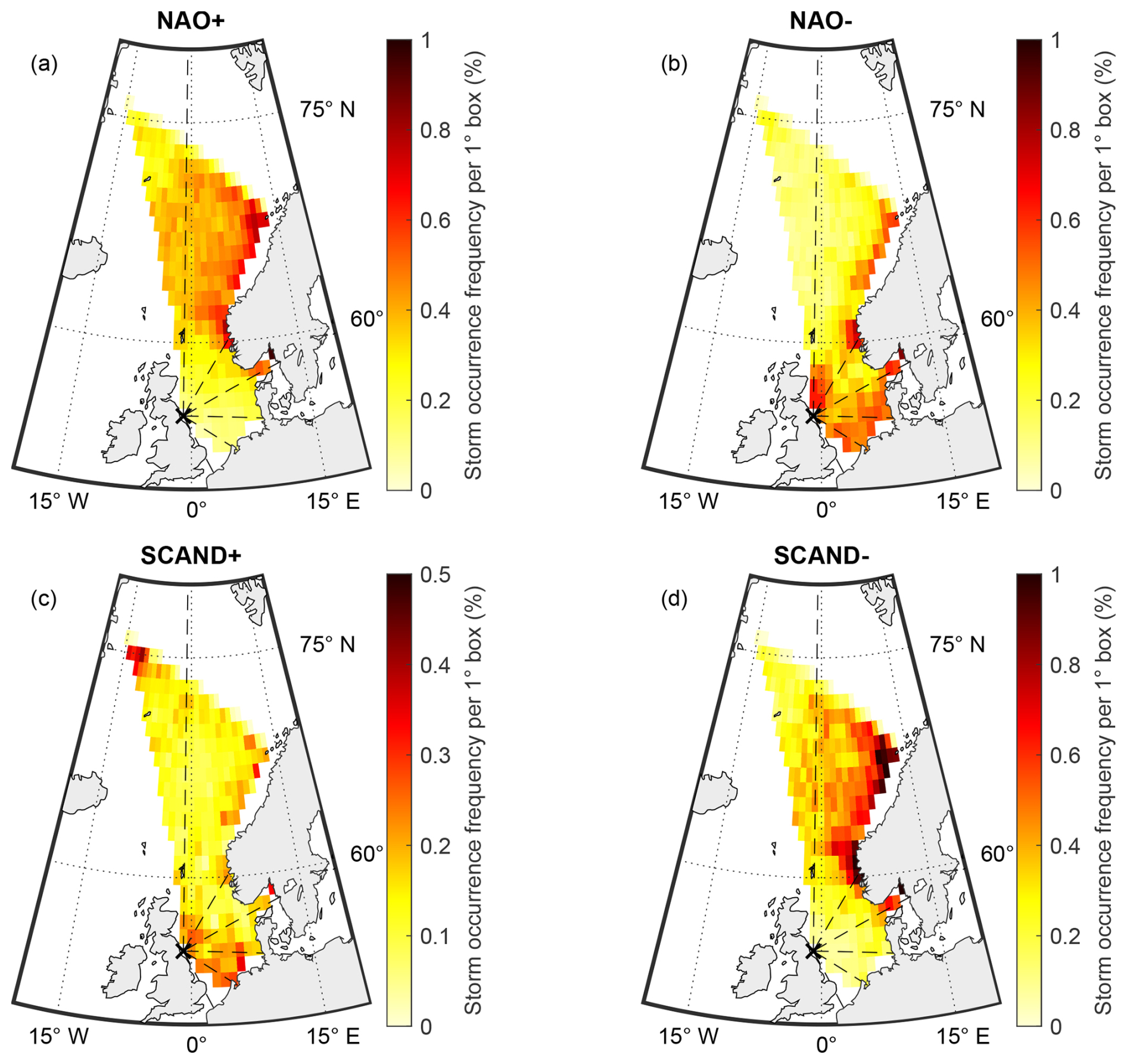
Figure 9 Spatial distribution of storm occurrence frequency associated with WTs that occur more frequently during each climate index phase. For each 1°×1° grid box, the storm frequency is calculated by the number of hours with storms detected divided by the total number of hours. The black cross indicates the study location. Radial black dashed lines originating from the study site indicate great circle paths at 30° intervals. Note that panel (c) uses a smaller colour-bar range than the others.

It is worth noting that the travel time of swell waves from their source regions to the study site is not accounted for in our analysis. As a result, the WT associated with a storm may differ from the WT associated with the resulting swell, which can arrive several days later. To assess the impact of this limitation, we also categorized the storms based on the monthly indices (i.e. independent of WTs) and calculated the spatial distribution of storm frequency for each climate index phase (Fig. A7). Months in which the index exceeded 1 standard deviation were classified as being in the positive phase, while those below −1 standard deviation were considered in the negative phase. As can be seen, no substantial differences in storm spatial patterns are observed between the two approaches across all index phases, suggesting that neglecting swell travel time does not influence our findings.

3.3.2 Storm surge

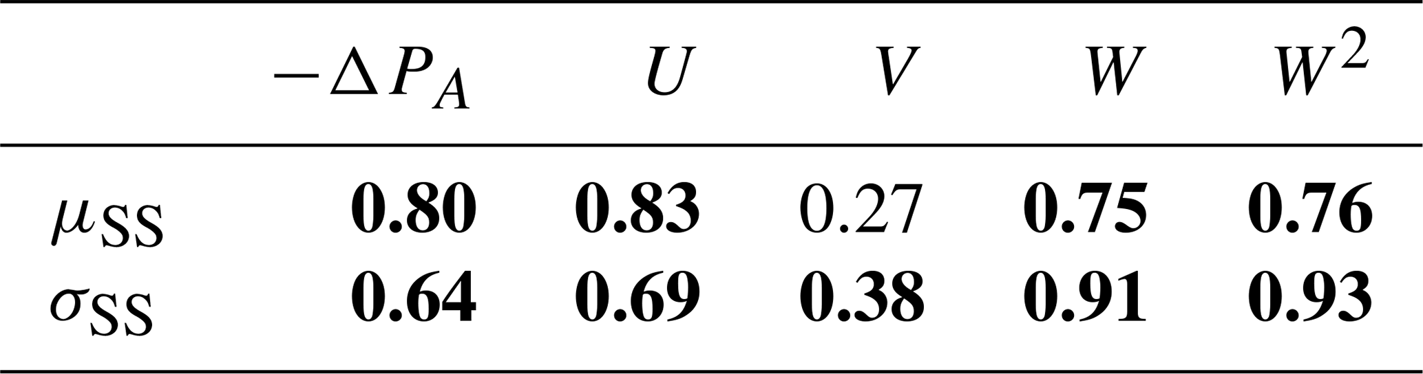
The response pattern of storm surge mainly lies in the position and shape of the storm surge distributions, which can be represented by μ_SS and σ_SS, respectively. To investigate the underlying drivers, a correlation analysis was performed between these distribution parameters and the effects of atmospheric processes (see Table 2). We found a strong correlation between μ_SS and the effects of both atmospheric pressure and wind stress. Among the wind parameters we considered, U displays the strongest correlation (0.83) while V is not significantly correlated. In addition, we calculated the storm surge caused by atmospheric pressure anomaly (Δη in Eq. 2) for each WT and compared it with the μ_SS of each storm surge distribution, with the Root Mean Square Deviation (RMSD) and BIAS provided (Fig. A8). Their definitions are given as follows:

$$\begin{array}{}\text{(4)}& {\displaystyle }& {\displaystyle }\text{RMSD}=\sqrt{{\displaystyle \frac{{\sum }_{i=\mathrm{1}}^n(x_i-y_i{)}^{\mathrm{2}}}{n}}},\text{(5)}& {\displaystyle }& {\displaystyle }\text{BIAS}={\displaystyle \frac{\mathrm{1}}{n}}\sum _{i=\mathrm{1}}^n(x_i-y_i),\end{array}$$

where x and y are a pair of random variables, n is the number of variable pair (equals the number of WTs). The result shows a good agreement, with the RMSD and BIAS being 7.19 and 1.57 cm, respectively. For σ_SS, the strongest correlation is found with W² (0.93).

Table 2 Pearson correlation coefficient between storm surge parameters related to each WT and parametrizations of atmospheric processes. Bold values indicate statistical significance (p-value<0.05).

4 Discussion

In this work, we investigated the link between large-scale climate modes and local wave climate and storm surge through WTs. We focused on two key climate indices, NAO and SCAND, as our correlation analysis identified both indices as being relevant to local sea state variability. This is consistent with previous studies, which have shown that NAO and SCAND contribute to sea level and wave climate variability in the North Sea and wider North Atlantic region (Shimura et al., 2013; Frederikse and Gerkema, 2018; Hochet et al., 2021; Casas-Prat et al., 2024). The direct correlation analysis identifies which climate indices are statistically related to local sea state variability at Hartlepool, whereas the WT analysis helps interpret how these relationships arise. In this sense, WTs are not used primarily to detect climate–sea state relationships; rather, they provide a probabilistic link between climate modes, atmospheric circulation patterns, and local wave and surge distributions.

4.1 The link between climate modes and wave climate

The relationship between ocean waves and climate modes has been widely discussed in previous studies, with a focus on H_s. A commonly observed pattern in the North Atlantic basin is that H_s tends to be positively correlated with the NAO index at higher latitudes, while showing a negative correlation at mid-latitudes (Shimura et al., 2013; Hochet et al., 2021). However, in the North Sea where the basin is more sheltered from the open ocean, the association between H_s and NAO is notably weaker, with the correlation in winter generally below 0.5 (Semedo et al., 2015). In our study, no significant link was found between H_s and NAO or SCAND through either correlation analysis (Table 1) or comparing the H_s distributions associated with each climate index phase. This does not imply that local wave climate is insensitive to these climate modes. Rather, the response is expressed more clearly through other wave characteristics.

First, we observed that local T_p distributions are bimodal during NAO+/SCAND− and near-unimodal shapes during NAO−/SCAND+. This pattern is likely attributable to the frequency of observing wind wave-dominated or swell-dominated wave spectra. During NAO+/SCAND−, the chance of the wave spectra at Hartlepool being dominated by either wind waves or swell is relatively comparable (around 56 % and 44 %, respectively), which leads to the formation of two distinct peaks in T_p distributions. On the other hand, during NAO−/SCAND+, the wave spectra are largely dominated by swell, resulting in a low probability of T_p falling in the wind wave range, which is insufficient to form a distinct secondary peak. This wave climate characteristic is different from the general pattern in the global open ocean, where the prevalence of swell is observed almost everywhere, even in mid to high latitudes along the extratropical storm tracks (Semedo et al., 2011). Our results suggest that the likelihood of wind wave dominance can exceed that of swell waves in more sheltered areas under NAO+/SCAND−. Semedo et al. (2015) also reported a lower frequency of swell-dominated wave fields in this region under NAO+, consistent with our findings.

Second, the wave directions vary between NAO/SCAND phases. The prevailing wind conditions under NAO+/SCAND− closely align with the primary wind wave directions, and this relationship remains robust throughout our sensitivity analyses. In contrast, during NAO−/SCAND+, local wind directions show greater variability and do not fully align with the corresponding wind wave directions. For swell waves, the dominant directions generally correspond to the regions with higher storm frequency in each climate index phase.

The WT analysis helps interpret why these phase-dependent wave responses arise, by showing how climate modes alter the occurrence probabilities of synoptic circulation patterns that favour different combinations of remote swell generation and local wind forcing. During NAO+/SCAND−, it is more likely to observe WTs characterized by intense low pressure systems centred near Iceland, the Norwegian Sea, or the Scandinavian Peninsula. These regions also correspond to areas of enhanced storm activity and are relatively distant from Hartlepool, allowing remotely generated waves to develop longer periods before reaching the site. Meanwhile, most of these WTs are also characterized by strong local south-westerly wind forcing across the UK, contributing to more energetic wind wave conditions. In comparison, WTs that occur more frequently during NAO−/SCAND+ are characterized by low pressure systems located at lower latitudes, mainly around the British Isles. Under these conditions, the North Sea becomes a more important source region for swell generation. Because this source region is closer to Hartlepool, the resulting swell is likely to have shorter propagation distances and therefore less time to develop into distinctly long-period waves. At the same time, the distribution of low pressure systems of these WTs is less spatially concentrated. This leads to larger variability in the orientation of pressure gradient, which favours less consistent wind wave directions.

4.2 The link between climate modes and storm surge

Storm surge characteristics in the North Sea generally display a positive correlation with the NAO index, with this association being stronger in the northeastern part of the basin, as revealed by previous research (e.g. Wakelin et al., 2003; Woodworth et al., 2007). Woodworth et al. (2007) further showed that the sensitivity to NAO differs between median and extreme storm surge conditions: SS₉₉ increases more than SS₅₀ for each unit increase in the NAO index. This difference in sensitivity can be explained by the change in the shape of storm surge distributions. Given that the storm surge associated with each WT approximately follows a normal distribution, SS₅₀ can be represented by μ_SS, whereas SS₉₉ is affected by both μ_SS and σ_SS. Since both μ_SS and σ_SS are positively correlated with NAO, a higher NAO index typically favours both a positive shift and widening of the distribution, thereby increasing SS₉₉ more significantly than SS₅₀. This may also explain the lack of significant correlation with SS₁, which is positively related to μ_SS but negatively to σ_SS. As such, the effects of μ_SS and σ_SS counteract each other, resulting in no significant change in SS₁ in response to NAO.

The response patterns of μ_SS and σ_SS are related to the effects of local atmospheric pressure and wind stress, both of which are modulated by large-scale climate modes. During NAO+/SCAND−, WTs characterized by negative pressure anomalies over Hartlepool and stronger winds occur more frequently. Similar synoptic conditions have been reported in previous studies (e.g. Gleeson et al., 2019; Scott et al., 2021). These conditions contribute to the increase in μ_SS and σ_SS, producing SS distributions that are more widely spread and shifted toward positive values. In comparison, WTs occurring more frequently during NAO−/SCAND+ are generally associated with positive pressure anomalies and weaker winds over the study region. These conditions favour lower μ_SS and reduced σ_SS, resulting in SS distributions that are more narrowly centred around zero.

4.3 Implications

The added value of this study arises from combining weather typing with a multivariate characterization of sea state conditions, including the partitioning of the wave field into wind wave and swell components. The WT framework provides a probabilistic link between climate modes, synoptic circulation patterns, and local sea state distributions, while the partitioned wave analysis reveals response features that would not be evident from the combined wave fields. A further advantage of this approach is its ability to capture response patterns through full distributions rather than correlation coefficients alone, thereby offering a complementary perspective to conventional statistical analyses. For example, the modality of T_p distribution is linked with NAO and SCAND phases, a feature that cannot be captured by a simple correlation coefficient. The sensitivity of the mean and extreme storm surge to climate indices can be interpreted through the variations of mean and standard deviation of the storm surge distributions.

The WT-based approach also allows the investigation of the joint response of multiple sea state variables to climate modes using two-dimensional distributions. In this work, we demonstrated the joint response pattern of wave height and wave direction through wave rose diagrams (Fig. 6). It would also be interesting to examine whether climate indices modulate the probability of compound wave–surge events. In addition, the local tidal range varies from around 1–5 m. Incorporating tidal variability into such an analysis might further clarify whether extreme coastal water levels during particular climate index phases arise from the concurrence of multiple drivers or from the dominance of a single component. A comprehensive compound analysis of waves, surge, and tide is, however, beyond the scope of the present study.

Our findings show that weather types, despite representing synoptic conditions over relatively short time scales (4 d in our case), can effectively link interannual climate modes with local sea states. This provides a strong rationale for the construction of WT-based stochastic emulators of sea state conditions (e.g. Anderson et al., 2019; Cagigal et al., 2020). In these emulators, the impact of climate modes is reproduced through modelling the occurrence frequencies of WTs at different climate index phases, which in turn produce sea state variations at the corresponding time scales. Such emulators are designed to generate infinitely long time series of sea state conditions for coastal risk assessments (e.g. extrapolation of extreme conditions and evaluation of long-term risk evolution). Given the role of climate modes in modulating coastal hazards, it is important to incorporate their influence into the emulator to reproduce realistic time series of sea states.

Investigating the influence of climate modes through weather types is also relevant from a predictability perspective. Individual synoptic weather systems have limited predictability beyond weather-forecast timescales, whereas slowly varying climate modes may contain predictable components on seasonal to decadal timescales (Dunstone et al., 2016; Athanasiadis et al., 2020), although the level of skill varies among prediction systems and remains sensitive to the representation of North Atlantic ocean–atmosphere interactions (Patrizio et al., 2025). Establishing how such climate modes alter the occurrence probabilities of synoptic circulation patterns and associated local sea states could therefore provide a basis for translating large-scale climate predictions into probabilistic information on coastal wave and storm surge conditions.

4.4 Regional applicability of results

The weather types developed in this study are tailored to the specific location using regression-guided classification to enhance downscaling performance. However, this also implies that caution should be exercised when transferring the results to other regions, particularly those with distinct geographic or oceanographic characteristics. To assess the broader applicability of our results, we calculated spatial correlations of sea state parameters across the North Sea relative to our study location (Fig. 10). The offshore wave and storm surge conditions along the north-east coast of England exhibit very high correlations (>0.9), which indicates similar response patterns associated with climate modes. This regional coherence in sea state variations was also reported in Scott et al. (2021). The correlations decrease with increasing distance from the study location, but the rate of decline varies among sea state parameters. Storm surge correlations remain relatively high (>0.8) across the south of the North Sea, whereas wave parameters exhibit a more rapid spatial decay. This suggests the response patterns of storm surge are transferable over a larger region than those of the wave climate.

Although the design of this research is inherently site-specific, the weather typing method itself is applicable to any location. To extend the analysis to multiple sites in a region, a single set of weather types can be developed using unsupervised classification (i.e. without tailoring to specific sites) to ensure consistency and comparability across locations. Alternatively, the weather types can be tailored to represent sea states over a larger region using the approach described by Zhao et al. (2024), which allows the investigation of the spatial variations in the impacts of climate modes.

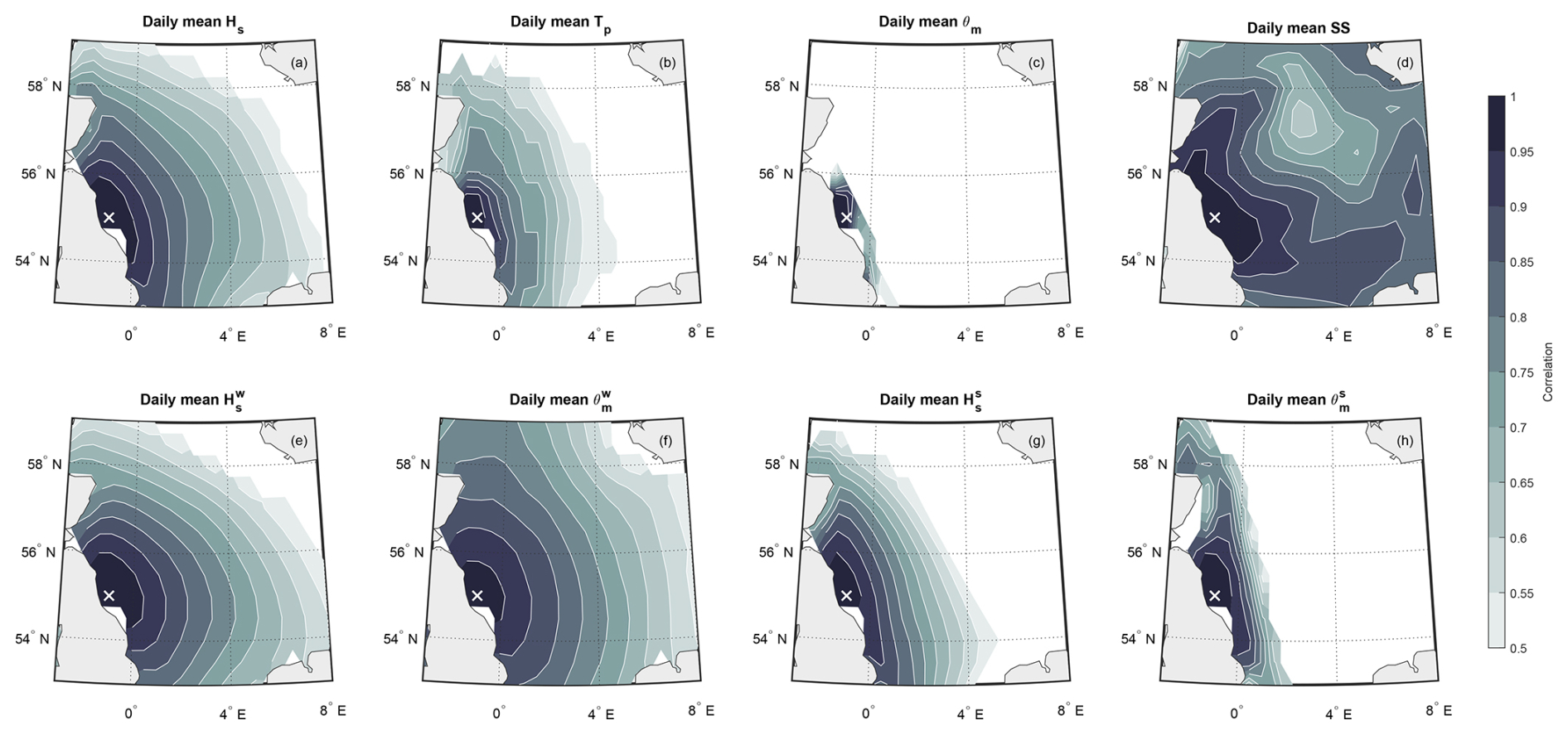
Figure 10 Spatial correlations of sea state parameters across the North Sea relative to our study location (indicated by a cross mark). Pearson correlation was calculated for scalar quantities, while a circular–circular correlation (Berens, 2009) was used for circular variables (i.e. wave directions). Daily mean parameters during DJFM for the period 1979–2018 were considered. Areas with no data or with correlations below 0.5 are not shown.

5 Conclusions

In this study, we investigate the link between climate modes and local wave climate and storm surge conditions at Hartlepool. Our first objective is to identify the climate modes contributing to the local sea state variability, which was achieved through a correlation analysis between six climate indices and wave and surge variables. Statistically significant correlations were found for NAO, SCAND, AO, and WEPA, with the first two selected for further analysis.

Our second objective focuses on characterizing the responses of wave and storm surge under the positive and negative phases of NAO/SCAND, where the WTs were introduced. WTs and their associated sea state distributions were related probabilistically to each phase of NAO/SCAND based on WT occurrence probabilities. The main findings are as follows: (1) the overall T_p distribution for WTs occurring more frequently during NAO+/SCAND− displays bimodality, while the distribution related to WTs occurring more often during NAO−/SCAND+ tends toward a unimodal pattern; (2) the wave energy spectra are more frequently dominated by wind waves during NAO+/SCAND− and by swell during NAO−/SCAND+; (3) the distributions of ${\mathit{\theta }}_m^w$ and ${\mathit{\theta }}_m^s$ show distinct patterns regarding the dominant direction between climate index phases; (4) the SS distributions for WTs occurring more frequently during NAO+/SCAND− have higher means and standard deviations than those occurring more frequently during NAO−/SCAND+.

The final objective investigates the atmospheric processes linking climate modes to the observed sea state responses. We parametrized the impacts of prevailing wind conditions, extratropical storms, and atmospheric pressure and related them to local sea state variability. Our analysis suggests that WTs that occur more frequently during NAO+/SCAND− are characterized by stronger westerly winds, enhanced storm activity at higher latitudes, and more negative local pressure anomalies. These conditions favour a combination of locally generated wind waves, remotely generated longer-period swell, and storm-surge distributions with higher means and greater variability. In contrast, WTs occurring more frequently during NAO−/SCAND+ are generally associated with weaker and more variable local winds, storm activity concentrated closer to the North Sea, and more positive pressure anomalies. These conditions favour a greater relative contribution from swell generated nearer to the site and storm surge distributions with smaller means and reduced variability.

Our research demonstrates the value of weather typing as a physically interpretable layer connecting large-scale climate modes, synoptic atmospheric circulation, and local sea-state distributions. Although this study focuses on Hartlepool, the method is widely applicable to other locations, and the findings are particularly relevant to sites along the north-east coast of England. More broadly, linking potentially predictable climate modes to the occurrence probabilities of WTs may support the translation of seasonal-to-decadal climate information into probabilistic estimates of coastal wave and storm-surge conditions for long-term planning and risk assessment.

Appendix A: Additional figures

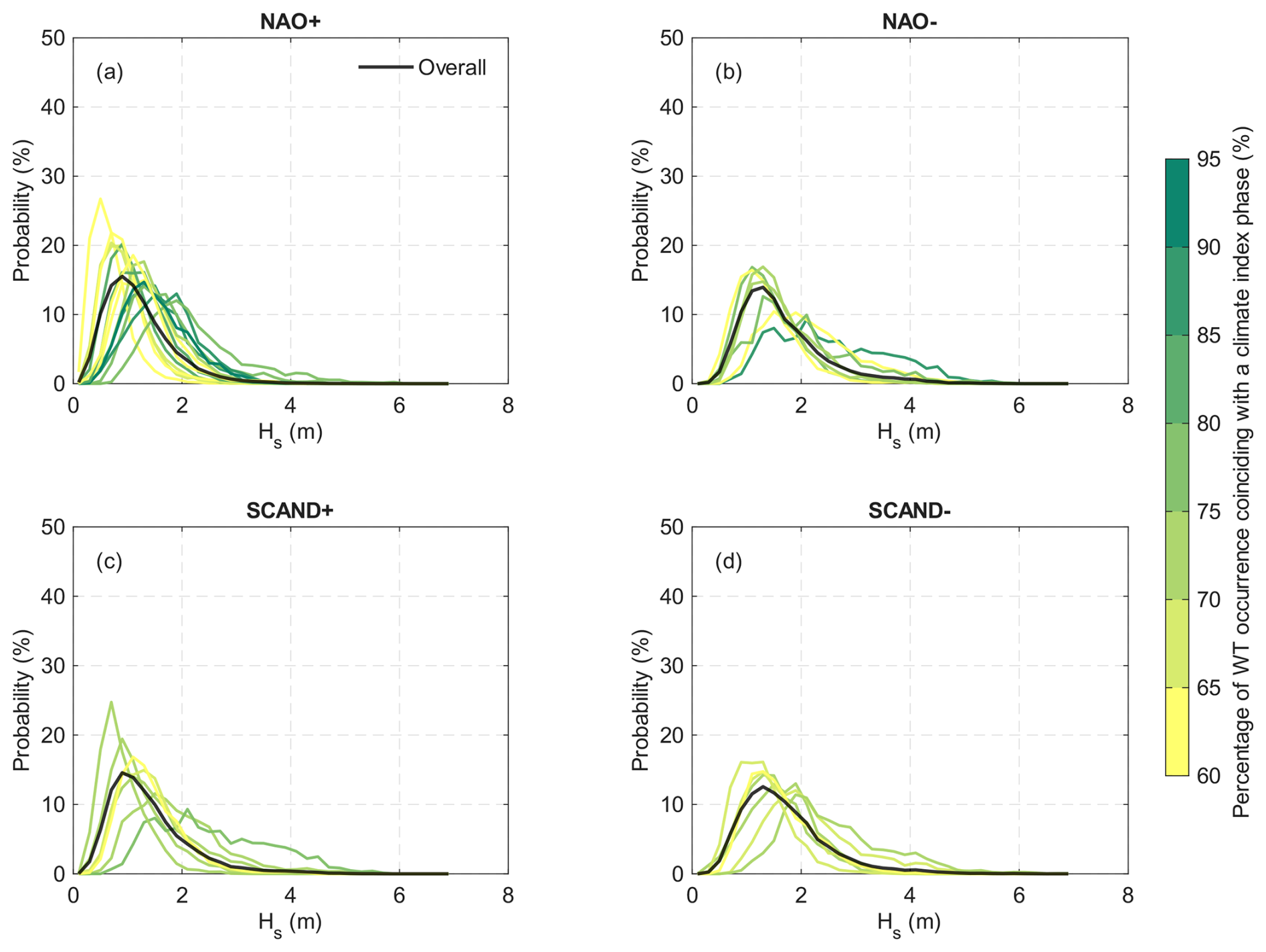
Figure A1 The empirical distributions of hourly H_s associated with WTs that occur more frequently during each climate index phase. Each coloured distribution is associated with an individual WT, with the colour representing the percentage of WT occurrence in particular NAO or SCAND phases in Table B1, thus indicating the strength of the association. The overall distributions (black) are derived from all hourly H_s values from WTs assigned to the same category of index phase.

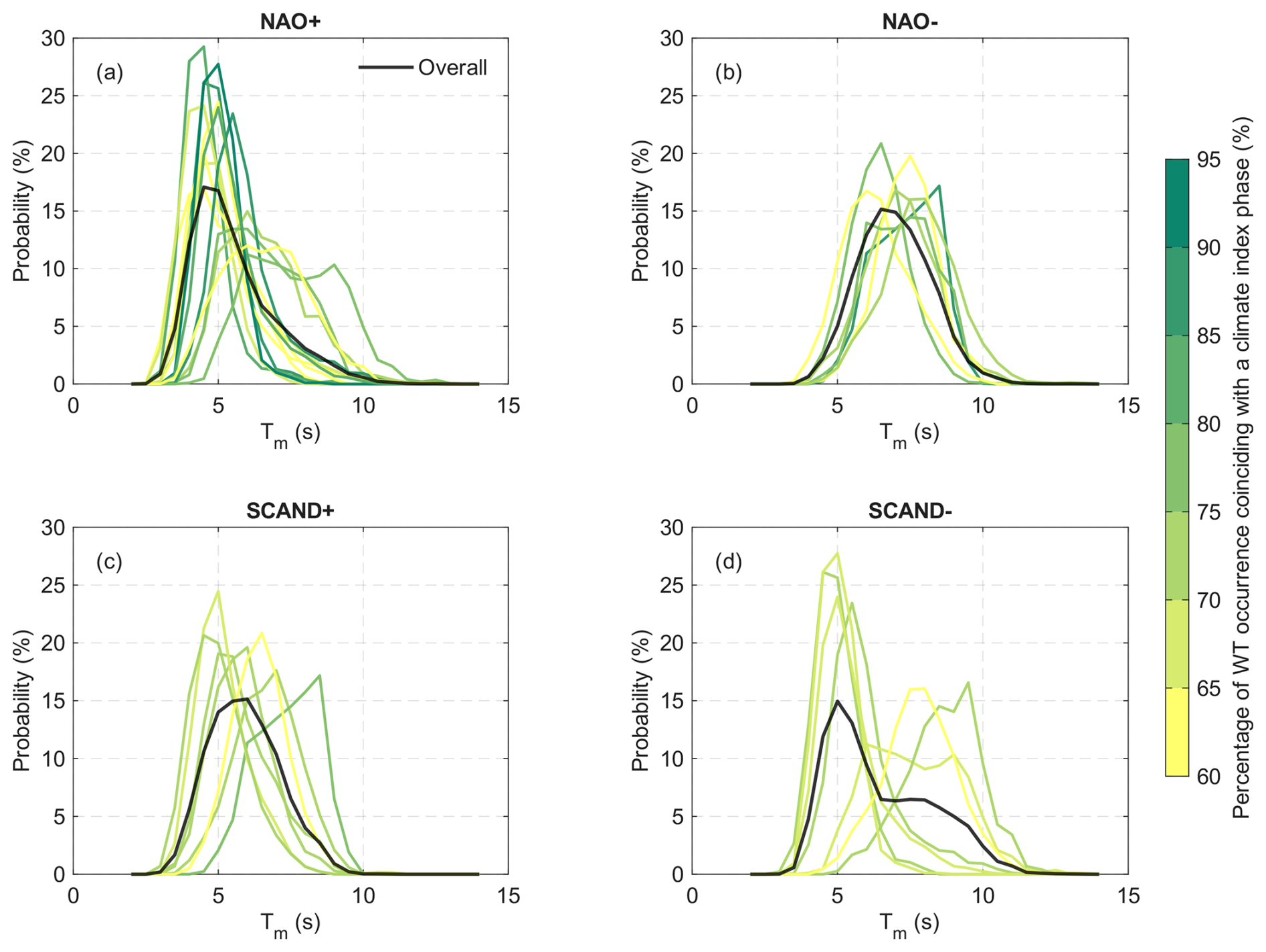
Figure A2 The empirical distributions of hourly T_m associated with WTs that occur more frequently during each climate index phase (similar to Fig. A1).

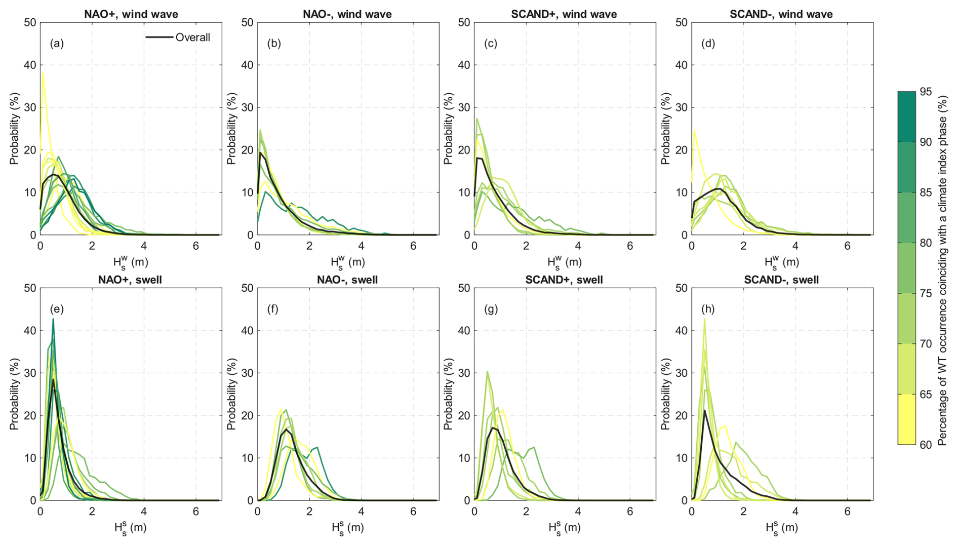
Figure A3 The empirical distributions of hourly $H_s^w$ and $H_s^s$ associated with WTs that occur more frequently during each climate index phase (similar to Fig. A1).

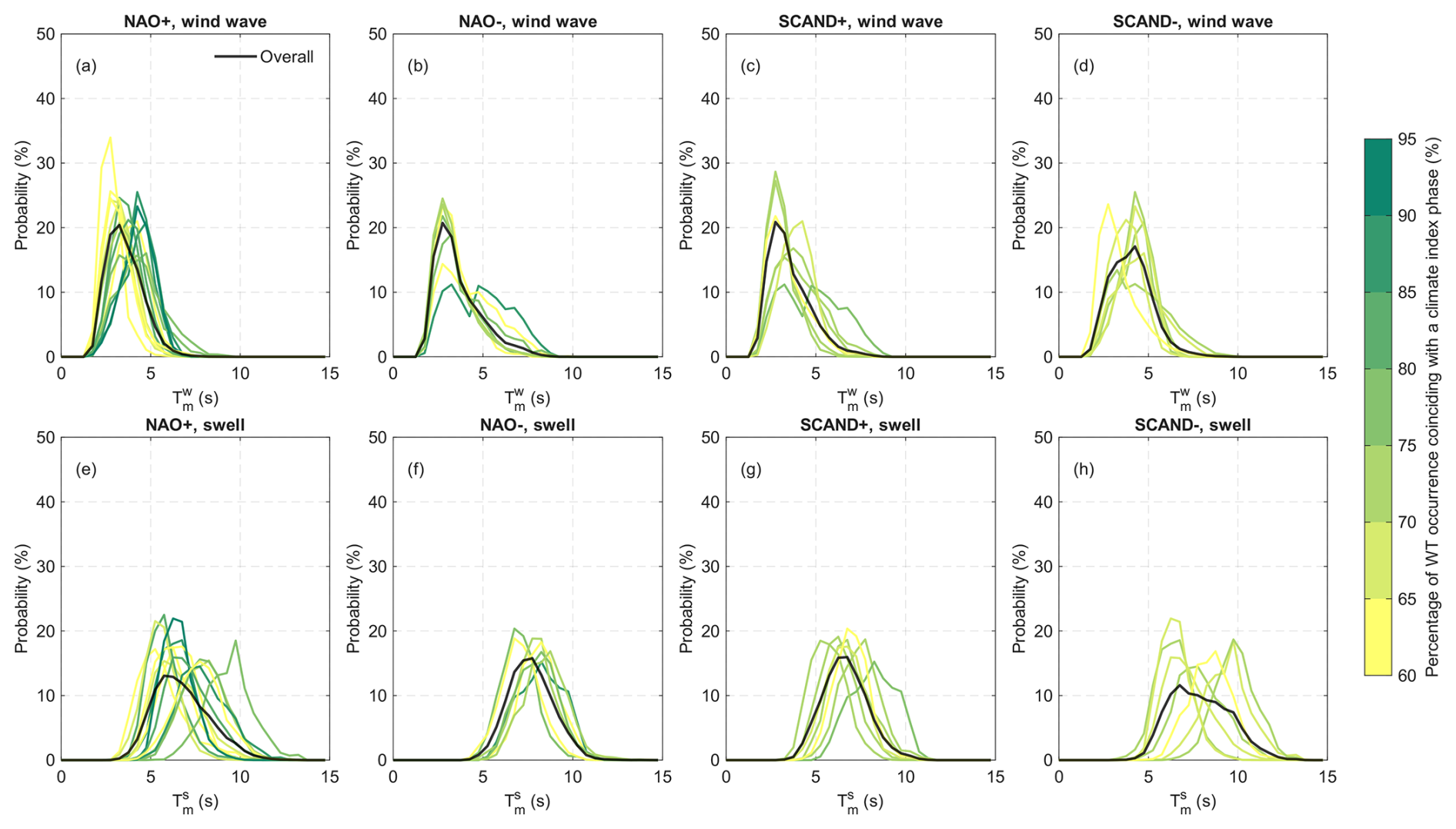
Figure A4 The empirical distributions of hourly $T_m^w$ and $T_m^s$ associated with WTs that occur more frequently during each climate index phase (similar to Fig. A1).

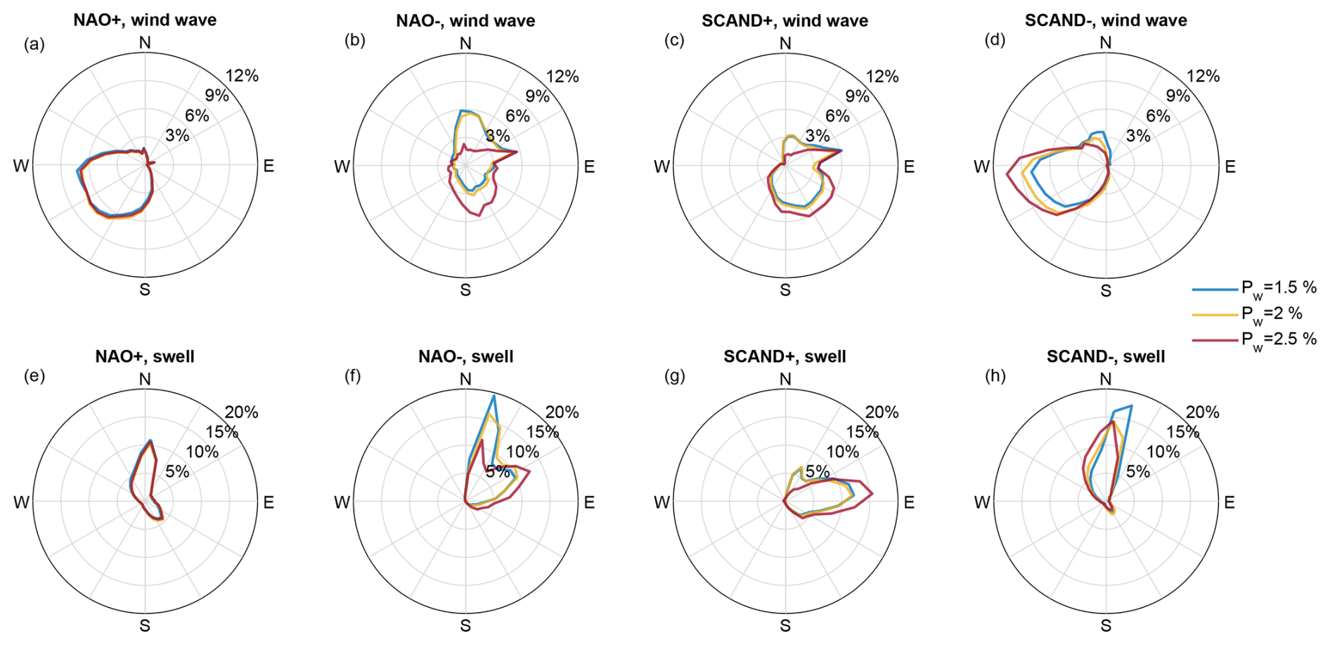
Figure A5 Sensitivity analysis of the impact of P_w in WT categorization on wave direction distributions.

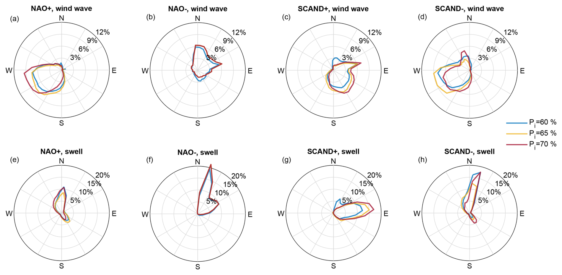
Figure A6 Sensitivity analysis of the impact of P_i in WT categorization on wave direction distributions.

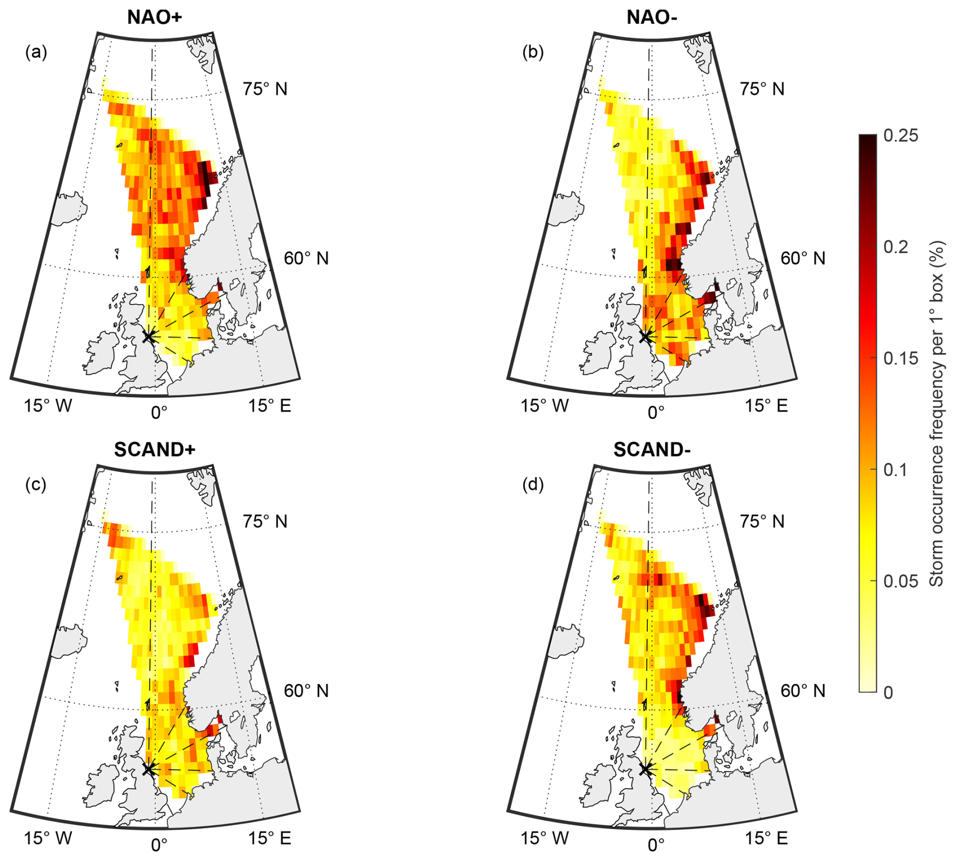
Figure A7 Spatial distribution of storm occurrence frequency associated with NAO and SCAND index phases, similar to Fig. 9. The association of storms with index phases is based on monthly climate indices, not weather types.

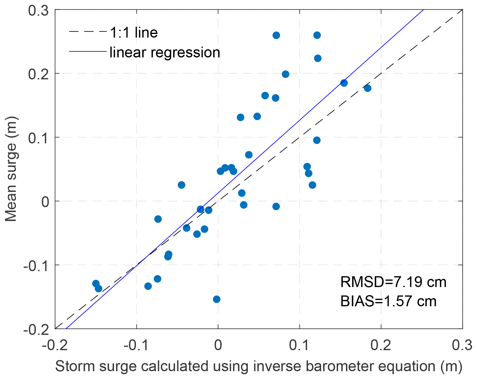
Figure A8 Comparison between estimated storm surges caused by the inverse barometer effect and the mean of storm surge distribution associated with each WT.

Appendix B: Additional tables

Table B1 WT categorization based on the percentage of occurrence coinciding with a positive or negative index during DJFM.

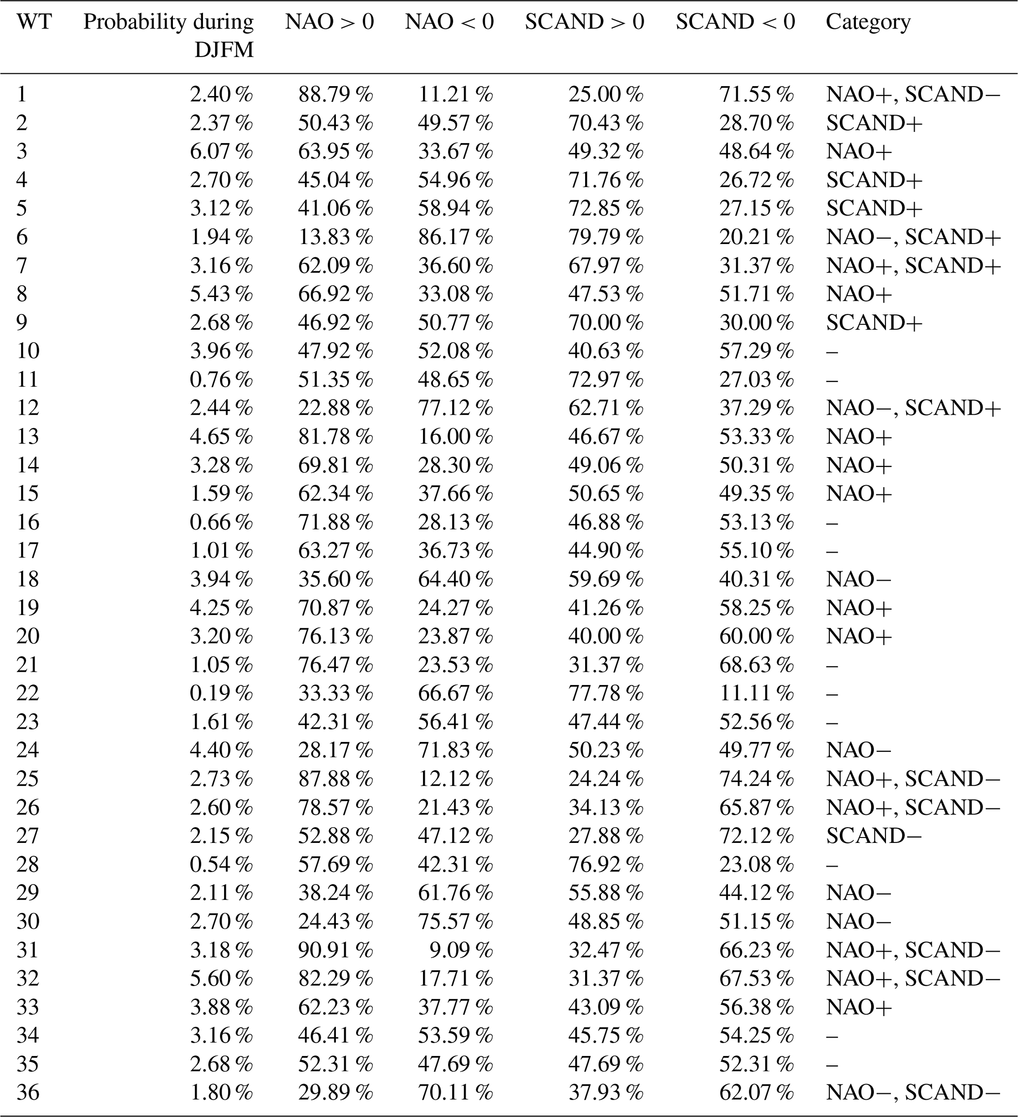
Table B2 Distributions and statistics of $H_s^w$ and $H_s^s$ associated with WTs that occur more frequently during each climate index phase. Pr{X} denotes the occurrence probability of X.

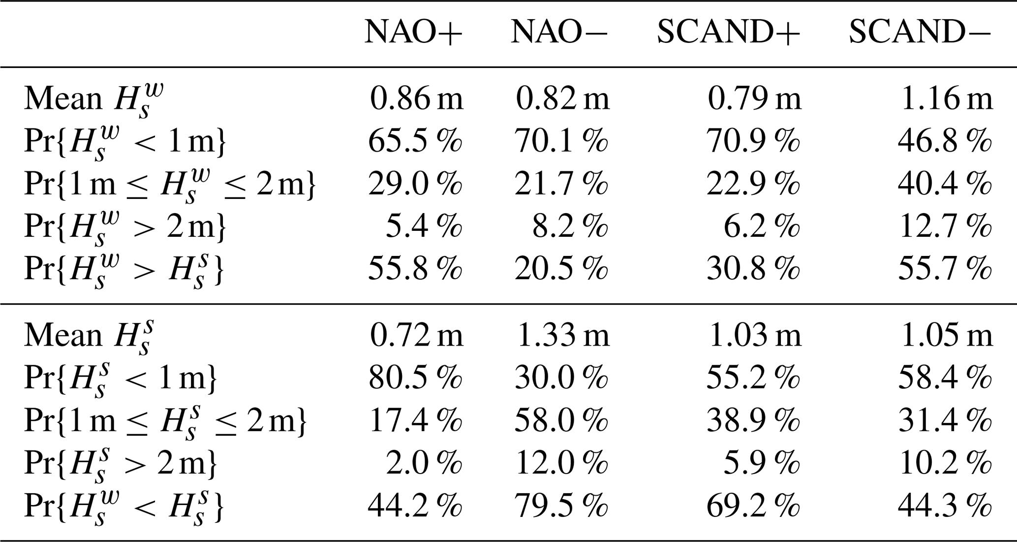
Table B3 Sensitivity analysis of the method for associating WTs with climate index phases. The influence of the two threshold values on storm surge and wave climate characteristics linked to NAO and SCAND phases was evaluated. In the baseline case, P_w and P_i are set to 1.5 % and 60 %, respectively (i.e. the values used in Table B1).