Improving ocean bottom pressure fields using space gravity data in state estimation

Ocean bottom pressure (p_b) is critical for monitoring and understanding ocean variability, yet global observations from GRACE and GRACE Follow-On suffer from limited spatiotemporal coverage. State estimation methods allow for the dynamical interpolation of sparse data by optimally combining observations with models. Here we examine the effects of assimilating GRACE data (local p_b anomalies and global mean), along with other datasets, on state estimates produced by the project for Estimating the Circulation and Climate of the Ocean (ECCO). The ECCO optimization leads to large adjustments in p_b fields at monthly and longer timescales. A substantial part of those adjustments is directly induced by GRACE constraints, with largest impacts occurring at high latitudes. Additionally, the mean ocean mass constraint is essential for mitigating large imbalances in freshwater fluxes derived from atmospheric reanalyses (used as prior forcing) and for producing a realistic barystatic sea level curve. Interpretation of remaining ECCO and GRACE differences highlights issues with non-oceanographic data signals. Our findings indicate that GRACE data contain information complementary to that available in other datasets, quantifying their value for determining p_b and associated circulation fields.

1 Introduction

Extensive knowledge and understanding of the ocean surface pressure field, as given by the difference between sea level and the geoid, has accumulated since the advent of high-quality satellite altimetry in the early 1990s (e.g., Stammer and Cazenave, 2017). Much less is known, however, about the ocean bottom pressure fields p_b. In contrast with the numerous altimeter missions flown since 1992, GRACE (Tapley et al., 2004) and GRACE Follow-On (Landerer et al., 2020), hereafter referred to simply as GRACE, are the only space-based missions delivering variable p_b fields on the global scale since 2002. Available in situ p_b measurements offer extremely limited spatial and temporal coverage and are also susceptible to long-term drift. The GRACE observations of p_b have been very useful to monitor and understand changes in sea level (e.g., WCRP Global Sea Level Budget Group, 2018), ocean heat content (e.g., Hakuba et al., 2024), ocean circulation (e.g., Landerer et al., 2015; Makowski et al., 2015), and other important climate-related issues. Nevertheless, their relatively coarse spatial resolution can be a limiting factor when trying, for example, to close regional sea level budgets (e.g., Ponte and Schindelegger, 2024) or measure changes in circulation involving narrow boundary currents (e.g., Landerer et al., 2015).

Models can provide dynamical interpolation of sparse data in both space and time. In particular, formal data assimilation methods allow for the optimal combination of observations and models to address some of the shortcomings of both. While altimeter data are routinely assimilated in most ocean analyses, relatively few efforts have used space-based p_b fields in a similar way. Early attempts by Köhl et al. (2012) used GRACE monthly data constraints for the period 2003–2007 to demonstrate their significant impact on p_b variability and related barotropic streamfunction and transports, particularly in subtropical gyres, near boundary currents, and also in polar latitudes. Their findings indicated that GRACE data can contain information not otherwise available in altimetry and hydrography data, in part because of the vastly different eddy “noise” affecting the various datasets. Saynisch et al. (2015) focused on daily GRACE data and a slightly longer period (2003–2009) and confirmed the substantial effects of p_b constraints in the high latitudes, primarily associated with induced changes in barotropic wind-driven dynamics. Their ensemble Kalman filter was also able to filter out the correlated data errors (“striping”) that plagued many of the early spherical harmonic GRACE data products (Swenson and Wahr, 2006).

Despite these early findings, most widely used ocean reanalyses still do not assimilate any GRACE data (Storto et al., 2024). A notable exception is the project for Estimating the Circulation and Climate of the Ocean (ECCO; Wunsch et al., 2009). In addition to using local p_b anomalies, ECCO also uses GRACE-based estimates of global ocean mean mass to constrain the net freshwater flux into the oceans and associated changes in barystatic sea level (Gregory et al., 2019). The latest publicly released ECCO solution (Fukumori et al., 2019) assimilates the whole GRACE record, along with many other ocean datasets. Such estimates provide an excellent opportunity to reexamine the value of space-based p_b data for improving our grasp of the global p_b fields, in the broader context of the variable ocean circulation.

In this study, we first determine the effects of the comprehensive ECCO optimization on the p_b fields by comparing a recent ECCO solution to its corresponding forward-model run that is not constrained by any data. We examine separately local p_b anomalies relative to the spatial means, which are relevant for the study of the ocean circulation and dynamics (Sect. 3), and the spatial means themselves associated with barystatic sea level (Sect. 4). Comparisons with GRACE establish the positive effects of the optimization in reducing differences with the data, which are discussed in the context of assumed data errors (Sect. 3.1). After analyzing the spatiotemporal characteristics of the adjustments to the p_b fields resulting from the full optimization (Sect. 3.2), the direct influence of GRACE data constraints on the ECCO solution is ascertained by contrasting p_b adjustments during periods with and without GRACE data (Sect. 3.3). The importance of GRACE constraints on barystatic sea level are discussed in Sect. 4. Interpretation of GRACE misfits remaining after the optimization is offered in Sect. 5. A section with a summary of results and brief discussion of some future implications concludes the paper.

2 Model, data and methods

We deal primarily with p_b fields in this work. For convenience, throughout the rest of the paper we express p_b values in terms of manometric sea level (Gregory et al., 2019), in units of length (equivalent water thickness). The conversion involves division of pressure values by a mean seawater density (1029 kg m⁻³) and the acceleration of gravity (9.81 m s⁻²) (Gregory et al., 2019).

2.1 ECCO solution

Forget et al. (2015) provide a comprehensive treatment of ECCO Version 4 as a framework for global ocean state estimation. The ECCO Version 4 system combines the Massachusetts Institute of Technology general circulation model with a variety of ocean observations to produce estimates of the global ocean and sea ice state that are both a “best” fit to the data and an exact solution of the model equations. The non-linear optimization procedure is based on the method of Lagrange multipliers (aka adjoint method) and involves iterations of forward and adjoint model runs to minimize a cost function representing misfits of all observations and the model. The minimization is achieved through adjustments in control parameters, which in the case of ECCO Version 4 include atmospheric forcing fields, initial conditions, and internal mixing coefficients. For full details on the ECCO Version 4 assimilation platform, please refer to Forget et al. (2015).

In the minimization procedure, the cost function terms are based on the variance of the model-data differences divided by the square of the data errors. The latter, aside from instrument noise, include representation errors – “true” signals in the data that cannot be represented by the model (e.g., mesoscale eddies missing in coarse resolution models). In the particular case of the GRACE data relevant to our analysis, the estimated error standard deviation used in the optimization, shown in Fig. 1a, was derived by comparing the GRACE data against previous ECCO solutions following the methods detailed in Quinn and Ponte (2008) and Fukumori et al. (2018). Errors vary from a minimum of 1 cm, explicitly set to match typical GRACE error estimates (e.g., Quinn and Ponte, 2008; Watkins et al., 2015), to a few centimeters. Large values in the eastern tropical Indian Ocean, Gulf of Thailand, and near Japan, are the imprints of the strong Sumatra-Andaman and Tohoku earthquakes that are not fully corrected in the GRACE inversions and thus leak into the p_b fields – a clear example of representation error. Another example of such errors is the enhanced values in regions such as the Argentine Basin and the Agulhas Retroflection, which seem to be affected by ocean intrinsic variability associated with eddies and other nonlinear processes that cannot be represented in the coarse grids (nominally 1°) of the model used in the ECCO estimates (Zhao et al., 2021). Enhanced values in other areas (Red Sea, Gulf of Carpentaria, Baffin Bay, Kara Sea) may reflect higher data noise related to similarly enhanced p_b variability (Fig. 1b) or other representation issues as discussed in Sect. 5.

Figure 1 Standard deviation of (a) estimated GRACE error, and p_b fields for (b) GRACE data, (c) control run and (d) ECCOv4r5, based on their overlapping period, all in units of cm. Global spatial means have been removed from all the fields prior to the calculation of standard deviations.

The present analyses are based on the ECCO Version 4 Release 5 (ECCOv4r5) product – a basic extension of the publicly available Release 4 described in detail by Fukumori et al. (2019). Major differences in ECCOv4r5 include: an extended analysis period (January 1992–December 2019; Release 4 ends in December 2017); atmospheric forcing fields optimized from the Modern-Era Retrospective Analysis for Research and Applications Version 2 (MERRA-2; Gelaro et al., 2017) as the first guess; an adjointable sea ice thermodynamics model; Antarctica iceberg melting; and explicit treatment of ice shelf cavities (Nakayama et al., 2024). The ECCOv4r5 solution is constrained by most available observations listed in Fukumori et al. (2019). Aside from sea level, sea surface temperature and salinity data from satellites, and extensive use of in situ observations from Argo and other platforms, ECCOv4r5 includes p_b fields derived from GRACE and also GRACE Follow-On, which launched in May 2018. The p_b data, processed as detailed in Fukumori et al. (2018), were assimilated as monthly fields with respective global spatial means removed but otherwise retaining full temporal variability including trends. In the ECCO estimate, the effective spatial resolution of the GRACE data is approximately 300 km, achieved through the method described in Appendix E of Forget et al. (2015). All GRACE data, including those near coastal regions, are used to constrain the estimate. In addition to the GRACE and other datasets documented in Fukumori et al. (2019), ECCOv4r5 is also constrained by estimates of Antarctic ice-shelf melt (Rignot et al., 2013; Nilsson et al., 2022) by adjusting the heat transfer coefficient between ice-shelf and ocean (Nakayama et al., 2024); these adjustments affect the freshwater flux (and heat flux) associated with the ice-shelf melt, but not salt flux because the salinity of ice-shelves is assumed to be zero.

For comparison with the optimized ECCOv4r5 solution, we also consider output from the respective control run (ECCOctrl), which consists of a forward model simulation using prior (unadjusted) estimates of the control parameters. Differences between ECCOv4r5 and ECCOctrl quantify the impact of the data constraints and optimization procedures on the estimated fields. In the same manner, we use Version 4 Release 1 and its control run, described in detail by Forget et al. (2015), to examine p_b adjustments in an optimization that involved most of the data constraints applied in ECCOv4r5 but excluded the GRACE data.

2.2 Bottom pressure data

We use global p_b estimates from GRACE mass concentration (mascons) fields provided by the Jet Propulsion Laboratory (JPL; Version RL06Mv02V; filename GRCTellus.JPL.200204_202001.GLO.RL06M.MSCNv02CRI.nc; Watkins et al., 2015; Wiese et al., 2019). These data were used to constrain ECCOv4r5 and are thus most appropriate for our analyses. We note that version RL06Mv02V has since been retired and replaced by more recent versions, but changes between different versions are relatively small and calculations using more recent versions did not lead to any meaningful differences in our findings. In this context, because the barystatic sea-level curve corresponding to the RL06Mv02V mascon fields could not be found in the GRACE Tellus archives, we chose to use one from the Wiese et al. (2024) dataset, which is a more recent version of JPL mascon fields but similar to the RL06Mv02V dataset. The global ocean mass is computed by summing up mass anomalies over the ocean and removing the mass of the atmosphere.

Variability in p_b estimates derived from GRACE can be related to non-oceanographic geophysical processes, such as those due to changes in gravity, rotation and deformation (GRD) effects defined in Gregory et al. (2019) and associated with variable mass loads (air, water and ice) over land. To evaluate the impact of these processes on our ECCOv4r5 and GRACE analyses, we take advantage of recent estimates of GRD effects by Landerer and Wiese (2025). The product provides global, monthly gridded solutions to the sea level equation (GRD components), derived from JPL CRI-filtered GRACE mascon surface mass anomalies from April 2002 to present. (These GRD corrections were not available at the time ECCOv4r5 solution was derived. Thus, uncorrected GRACE data was used in the ECCOv4r5 optimization.)

3 Analysis of local p_b fields

In this section, we examine gridded p_b anomalies defined relative to the respective global means discussed in Sect. 4. The anomalies are used as separate constraints on ECCOv4r5 and represent the dynamically relevant p_b variability associated with changes in ocean circulation.

3.1 Basic effects of optimization on p_b fields

The standard deviations of the local p_b anomalies for GRACE, ECCOctrl and ECCOv4r5 fields (Fig. 1b–d) are mostly consistent, in terms of spatial patterns and amplitudes. Maxima occur in shallow coastal regions, along the Southern Ocean (particularly in the Bellingshausen and Australian-Antarctic Basins) and in the Arctic, and minima are present over most of the tropics. There are, however, visible differences in variability between ECCOv4r5 and ECCOctrl over many regions (e.g., weaker ECCOv4r5 variability in the Barents Sea, Hudson Bay, Australian-Antarctic Basin, stronger in the Beaufort Gyre, Indian Ocean). Many of these differences make ECCOv4r5 amplitudes more consistent with those of GRACE, but the opposite can also be true (e.g., relatively large variability near the Weddell Sea).

In areas of western boundary currents (e.g., Agulhas retroflection, Gulf Stream extension, Argentine Basin), GRACE fields look more energetic than both ECCOv4r5 and ECCOctrl, consistent with the presence in GRACE of the effects of intrinsic variability (Zhao et al., 2021). The imprint of eddies on p_b variability in these regions has been documented in studies based on in situ p_b observations (e.g., Hughes et al., 2007; Na et al., 2016; Androsov et al., 2020). Such intrinsic signals occur on a variety of spatiotemporal scales and can affect the GRACE data even if not fully resolved by the measurements. They cannot be represented in either ECCOv4r5 or ECCOctrl, however, and thus constitute representation errors that (1) partly contribute to the enhanced data errors in regions of strong unstable currents noted in Fig. 1a and (2) effectively down-weight the GRACE data in those areas during the optimization.

Apart from boundary current regions, strongest amplitude differences between GRACE and ECCO fields are found in the eastern tropical Indian Ocean and near Japan, however. The large GRACE variability, absent in both ECCOv4r5 or ECCOctrl, is the imprint of the large Sumatra-Andaman and Tohoku earthquakes discussed in relation to Fig. 1a.¹

Results in Fig. 1 hint at the impact of the optimization on the p_b anomaly fields, but a more quantitative assessment can be gleaned from the root-mean-square difference (RMSD; based on demeaned time series here and throughout the paper) between GRACE, ECCOctrl and ECCOv4r5 (Fig. 2). Differences between ECCOv4r5 and ECCOctrl (Fig. 2c) are not negligible compared to their variability in most of the global oceans (cf. Fig. 1c and d). Largest changes are seen in the Mediterranean Sea, Arctic Ocean and various sectors of the Southern Ocean, as well as several shallow, enclosed seas and gulfs. These regions also correspond to some of the largest decreases in RMSD in GRACE − ECCOv4r5 compared to GRACE − ECCOctrl (Fig. 2d). More generally, the mostly negative values in Fig. 2d (∼88 % of all the grid points) imply that RMSD values for GRACE − ECCOv4r5 are smaller than those for GRACE − ECCOctrl, i.e., ECCOv4r5 is for the most part closer to the GRACE data than ECCOctrl. Values $<-\mathrm{0.5}$ cm amount to 27 % of the grid points in Fig. 2d, and values over the Arctic and Southern Ocean average to −1.6 and −0.5 cm, respectively. The correlations of GRACE with ECCOv4r5 (not shown) are also higher on average by ∼0.1 than those with ECCOctrl. Thus, the RMSD and correlation analyses reveal relatively large changes in p_b fields and a closer fit to GRACE data brought about by the ECCO optimization.

Figure 2 Standard deviation of the difference p_b fields (a) GRACE − ECCOv4r5, (b) GRACE − ECCOctrl and (c) ECCOctrl − ECCOv4r5, based on their overlapping period. Global spatial means have been removed from all the fields. The difference (a) minus (b) is shown in (d). Negative values imply ECCOv4r5 is closer to the GRACE data than ECCOctrl. Units are cm.

Focusing on the RMSD for GRACE − ECCOv4r5 (Fig. 2a), largest values of ∼5 cm coincide with areas of large variability (e.g., Bay of Bengal/Andaman Sea, around Japan, Arctic coastal regions) and smallest values (<1 cm) occur over most of the tropics where variability is weakest (Fig. 1). These RMSD values are not small compared to the variability in either GRACE or ECCOv4r5, but they are for the most part comparable to the data errors used to weight the gravity data in the ECCOv4r5 optimization (Fig. 1a).

The costs, i.e., the normalized quadratic misfits that constitute the cost function described in Sect. 2.1, calculated as

$$\begin{array}{}\text{(1)}& {\displaystyle \frac{\mathrm{variance}(\mathrm{GRACE}-\mathrm{ECCO})}{(\mathrm{GRACE}\mathrm{error}{)}^{\mathrm{2}}}}\end{array}$$

(i.e., the square of the ratio of values in Fig. 2b and c to those in Fig. 1a) and shown in Fig. 3, provide a quantitative measure of how the optimization has consistently reduced differences to the data within respective data uncertainties. The relatively large costs (>2) in ECCOctrl observed at polar and subpolar latitudes, coastal areas and marginal seas are substantially reduced in ECCOv4r5 to values closer to 1, as expected in a converged optimized solution. There are, however, several areas with ECCOv4r5 costs considerably >1 (e.g., Siberian Shelf, Bering and Chukchi Seas, Hudson Bay, North Sea) that may suggest only partial convergence and/or underestimated data errors. The latter is plausibly the case for the large ECCOv4r5 cost values seen in the areas affected by the Sumatra-Andaman and Tohoku earthquakes. In contrast, there are many ECCOv4r5 and ECCOctrl cost values < 1 (histograms display peaks at values of ∼0.45 and 0.65, respectively; not shown) and particularly in tropical latitudes. This points to the possibility of overestimated data errors, which were set to a minimum of 1 cm (Fig. 1a).

Figure 3 Costs calculated as the variance of the differences between GRACE and (a) ECCOctrl and (b) ECCOv4r5 (i.e., values in Fig. 2a and b squared) divided by the square of the data error (values in Fig. 1a squared).

3.2 Nature of p_b adjustments

A more detailed examination of the changes in p_b fields brought about by the ECCO optimization can provide useful insight on the characteristics of some of the major errors in the ECCOctrl estimate and elucidate various important aspects of the optimization. We first examine separately the linear trends and mean seasonal cycle as two major components of the p_b variability.

Trends in Fig. 4 exhibit for the most part basin-scale patterns of the same sign but are considerably different among the three fields. In particular, ECCOctrl has largest trends in the Arctic, the Mediterranean, and several shallow seas and coastal regions (e.g., Hudson Bay and a substantial part of the eastern North American and Patagonian shelves), which are not present in the GRACE data. There are also relatively large trends tightly trapped to some coastal regions (e.g., southern Africa and southern Australia; Fig. 4c) that appear to be too small scale to be representable in GRACE. All these large ECCOctrl trends are mostly adjusted by the optimization, with ECCOv4r5 considerably closer to GRACE than ECCOctrl in those regions (cf. Fig. 4d and e). Strong large-scale adjustments can also be seen in the Atlantic sector of the Southern Ocean, where the mostly negative trends in ECCOctrl become positive in ECCOv4r5, mimicking more of the trend pattern seen in GRACE.

Figure 4 Trends of p_b fields for (a) GRACE, (b) ECCOv4r5, and (c) ECCOctrl, and respective differences (d) GRACE − ECCOv4r5, (e) GRACE − ECCOctrl, and (f) ECCOctrl − ECCOv4r5, all in units of cm yr⁻¹ and based on the ECCO and GRACE overlapping period.

In contrast, relatively large GRACE trends in the eastern tropical Indian Ocean and near Japan are not present in either ECCOctrl or ECCOv4r5. The apparent rejection of these GRACE trends in the optimization is consistent with the data weights in Fig. 1a and the non-oceanographic, earthquake-related nature of these signals, as already discussed. Similar rejection of GRACE trends occurs in other areas such as Baffin Bay and the eastern North Atlantic. These trends are partly related to GRD effects discussed in Sect. 5, which are present in the data but not physically modeled in ECCO. Yet other areas show trend changes from ECCOctrl to ECCOv4r5 that increase (rather than decrease) the differences with GRACE (e.g., shift from negative to positive trends in the Argentine Basin). Thus, observational constraints other than those from GRACE can also have an impact on the p_b trends, which is not necessarily consistent with the GRACE data.

The seasonal cycle is a main component of p_b variability (e.g., Ponte, 1999, Fig. 3). The mean seasonal cycle is defined as the average of all values for each calendar month from January to December. The standard deviations of the resulting 12-month mean series are similar among GRACE, ECCOctrl and ECCOv4r5 (Fig. 5a–c). Values range from <1 cm over most of the oceans to higher values (typically 1–3 cm) in subtropical and subpolar gyres, the Arctic and the Southern Oceans, and many coastal regions. The optimization produces sizable changes in the mean seasonal cycle (Fig. 5f)², particularly in those higher variability regions, with ECCOv4r5 considerably closer to GRACE than ECCOctrl (Fig. 5d and e). The improved data fit for ECCOv4r5 implies both stronger (e.g., Beaufort Gyre) and weaker (e.g., Australia-Antarctic basin) seasonal cycles produced by the optimization.

Figure 5 Standard deviations of the mean seasonal cycle in p_b fields for (a) GRACE, (b) ECCOv4r5, and (c) ECCOctrl, and of their respective differences (d) GRACE − ECCOv4r5, (e) GRACE − ECCOctrl, and (f) ECCOctrl − ECCOv4r5, all in units of cm and based on the ECCO and GRACE overlapping period.

Similar findings arise when examining the residual p_b variability upon removal of linear trends and mean seasonal cycles (Fig. 6). Again adjustments to ECCOctrl (Fig. 6f) are comparable in magnitude to the variability (Fig. 6b and c) and ECCOv4r5 is for the most part a better fit to GRACE (cf. Fig. 6d and e). Large differences in variability seen in the eastern tropical Indian Ocean and near Japan indicate remaining earthquake signals, which as expected are not removed by simply detrending over the full length of the GRACE record.

Figure 6 Standard deviations of the residual p_b time series obtained by removing the trends and the mean seasonal cycle for (a) GRACE, (b) ECCOv4r5, and (c) ECCOctrl, and of their respective differences (d) GRACE − ECCOv4r5, (e) GRACE − ECCOctrl, and (f) ECCOctrl − ECCOv4r5, all in units of cm and based on the ECCO and GRACE overlapping period.

Taken together, Figs. 4–6 indicate that adjustments in p_b occur over the full range of timescales contained in the records. Empirical ortoghonal function (EOF) analysis provides a concise description of not only the temporal but also the spatial nature of the p_b adjustments. Here, we use Python package “eofs v2.0.0” (Dawson, 2016) to calculate EOFs for the full ECCOctrl − ECCOv4r5 fields (extending over 1992–2019) for completeness, but an analysis restricted to the GRACE period, as in Figs. 4-6, yields similar results. When using the raw ECCOctrl − ECCOv4r5 fields, the first EOF basically reproduces the long-term trend pattern in Fig. 4f and accounts for $\sim \mathrm{2}/\mathrm{3}$ of the total variance (not shown). To focus on the remaining variability, the EOFs calculated using detrended fields are shown in Fig. 7. The seasonal cycle is dominant in modes 1 and 2, which contribute ∼38 % of the total variance; modes 3 through 5 account for another ∼20 % of the variance, with their principal components containing more mixed seasonal and nonseasonal variability compared to modes 1 and 2. In particular, mode 3 shows a strong loading in the Atlantic sector of the Southern Ocean and a change in trend around 2002, reflecting in part the effects of GRACE constraints on the trends in that region, discussed in relation to Fig. 4.

Figure 7 First five empirical orthogonal functions of the detrended ECCOctrl − ECCOv4r5 p_b fields based on the full 28-year record (1992–2019). Time series of principal components (PC) are in units of cm.

In terms of spatial structure, all EOFs in Fig. 7 exhibit basin-scale, same-sign patterns. For example, mode 1 consists mostly of an out-of-phase pattern between high latitudes and low and mid latitudes, and similarly for mode 2 between the Southern and Indian Oceans and the rest of the ocean. Similar large scale patterns are present in modes 3 through 5. The Arctic and Southern Oceans as well as some coastal regions feature prominently in the modes, with the loadings generally consistent with the magnitudes of the p_b adjustments in Figs. 5f and 6f.

3.3 Impact of GRACE data on optimization

Whether the p_b adjustments described in Figs. 4–7 can be associated with the impact of GRACE data constraints remains an important question. Common methods to examine such questions include data withdrawal experiments, where one might compare solutions optimized with and without GRACE constraints (e.g., Köhl et al., 2012). In this study, we do not use such specific experiments but instead take advantage of the fact that GRACE record only starts in 2002 and contains several gaps since its inception. This allows us to evaluate the p_b adjustments during periods when GRACE data is available versus when it is not. Notably, the principal components of all the EOFs in Fig. 7 generally show different and enhanced variability after around 2002 (e.g., larger seasonal adjustments in mode 1, marked change in trend in mode 3), which coincides with the beginning of GRACE observations.

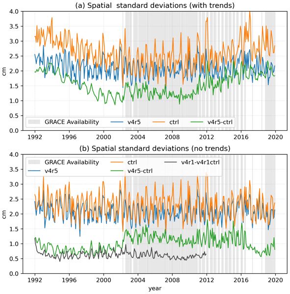
To ascertain the effect of the GRACE constraints, we calculate the spatial standard deviations of the ECCOctrl − ECCOv4r5 fields as a function of time (Fig. 8). Results based on the raw fields over the global ocean (Fig. 8a) show a bowl-shaped pattern of larger adjustments at the end points and minimum values in the middle of the record. This shape coincides with the behavior of the standard deviation of ECCOctrl p_b fields, also shown in Fig. 8a, in contrast with the rather flat nature of the standard deviation of ECCOv4r5 fields. Results based on detrended fields (Fig. 8b) show no bowl-shape characteristics for any curves. The changes to the linear trends in ECCOctrl brought about by the optimization (Fig. 4) are thus the main reason behind the larger adjustments at the end points for ECCOctrl − ECCOv4r5 curve in Fig. 8a.

Figure 8 Time series of the spatial standard deviation (cm) of the ECCOctrl − ECCOv4r5 p_b fields (green), calculated based on (a) full values and (b) detrended values. Black curve in (b) denotes the standard deviation of differences between ECCOv4r1 and respective control run for comparison. Shaded areas denote periods with GRACE data availability. Standard deviations of the corresponding p_b fields for ECCOctrl (orange) and ECCOv4r5 (blue) are also shown for context.

Once ECCOctrl − ECCOv4r5 fields are detrended, there is a clear tendency for larger p_b adjustments after GRACE data becomes available (Fig. 8b). The average value over months with GRACE data is 1.20 cm compared to 0.85 cm for months without it. Values over the ∼1-year gap between GRACE and GRACE-FO average to 0.72 cm, similar to levels prior to the onset of GRACE in 2002. Moreover, local minima tend to coincide with multiple shorter data gaps that occur particularly after 2011 until the demise of the GRACE mission in 2017. The consistently lower p_b adjustments over most data gaps, including that between GRACE and GRACE-FO, are strong evidence of the impact of the gravity data in ECCOv4r5. Calculations restricted to various latitude bands (not shown) yielded similar results, pointing to the effects of GRACE constraints over most regions.

Apart from the introduction of GRACE data in 2002, a major change in the observing system was the deployment of Argo floats, which started in the early 2000s and reached maturity during the second half of the decade. To assess whether such development could also contribute to the enhanced p_b adjustments after 2002, Fig. 8b shows the spatial standard deviations of the p_b adjustments based on the earlier Version 4 Release 1 fields, which included all the Argo data but not the GRACE data. The p_b adjustments for Release 1 show no visible enhanced values after the onset of Argo deployments and typical values similar to those associated with ECCOv4r5 results for periods without GRACE data. Thus impact of Argo data constraints on p_b are deemed not essential for explaining the behavior observed in the ECCOv4r5 results.

For a complementary analysis detailing regional influences, we calculate the difference in the temporal standard deviations of detrended ECCOctrl − ECCOv4r5 fields for periods with and without GRACE observations (Fig. 9). Again larger p_b adjustments are observed over most of the global ocean (∼87 % of the grid points) for periods with available GRACE data. Differences in adjustments > 0.5 cm are seen for ∼13 % of values, with largest differences occurring in the Arctic (near Franz Josef Land and in Beaufort Sea) and Southern Oceans and some marginal seas and coastal regions (e.g., Siberian Shelf, Bering and Chukchi Seas, Hudson Bay, North Sea, Japan/East Sea, Gulf of Thailand/South China Sea).

Figure 9 Difference in the temporal standard deviations of detrended ECCOctrl − ECCOv4r5 p_b fields, calculated for periods with and without GRACE observations. Positive values indicate larger p_b adjustments for periods with GRACE data.

The behavior of p_b adjustments implied in Figs. 8 and 9 (and also Fig. 7) is thus consistent with a direct impact of the GRACE data on the optimization of the ECCOv4r5 p_b fields. The differences in GRACE − ECCOv4r5 variability between periods with and without GRACE data are sizable compared to that of the p_b adjustments (cf. Figs. 9, 5f and 6f). While the influence of GRACE data on constraining long-term trends in p_b cannot be elucidated by our analysis, the impact on timescales ranging from monthly to interannual seems clear.

4 Global ocean mean mass analysis

The spatial mean of the p_b fields derived from GRACE provides an estimate of the changes in the global ocean mass including floating ice and snow, once effects of atmospheric mass over the ocean and other known geophysical effects like glacial isostatic adjustment are accounted for. In ECCOv4r5, total ocean mass is directly tied to precipitation, evaporation and runoff forcing, including exchange with icebergs and ice shelf cavities. The model employs the Greatbatch (1994) correction to ensure mass conservation. In the ECCOv4r5 optimization, global mean ocean mass and sea level were simultaneously brought into agreement with GRACE and altimetry estimates by adjusting the precipitation fields with a time-varying, spatially constant factor, while ensuring that such modified forcing did not incur any substantially larger costs for all the other data constraints in the system.

The spatial means representing total ocean mass estimated from GRACE, ECCOv4r5 and ECCOctrl are shown in Fig. 10, expressed in terms of the corresponding changes in barystatic sea level (Gregory et al., 2019). The ECCOctrl series exhibits a very different behavior from GRACE series, which reflects large imbalances in the net freshwater flux into the ocean, as estimated from the forcing fields provided by MERRA-2 reanalysis. The large negative trend in ECCOctrl series implies an ocean mass loss equivalent to a barystatic sea level drop of ∼30 cm over less than 2 decades, which is unrealistic in both sign and amplitude when compared to GRACE.

Figure 10 Global spatial means of raw p_b fields for GRACE data (blue), ECCOv4r5 (orange) and ECCOctrl (green), expressed as values of barystatic sea level (Gregory et al., 2019) in units of cm. The ECCO spatial means have been corrected for spurious changes resulting from the Boussinesq model physics and reflect the true net mass change due to net freshwater fluxes from evaporation, precipitation and river runoff, as well as from ice shelf cavities and icebergs.

In contrast, the ECCOv4r5 estimate of ocean mass is much more consistent with the observations, implying a barystatic sea level rise of ∼5 cm over the period examined (Fig. 10). There is also good agreement in their respective annual cycles. The RMSD between ECCOv4r5 and GRACE is ∼3 mm, similar to the estimated errors in GRACE of ∼2 mm (Quinn and Ponte, 2008; Fukumori et al., 2018). Thus, ECCOv4r5 provides a reasonable fit to the GRACE series within its expected uncertainty.

5 Interpretation of GRACE misfits

The focus in previous sections has been on contrasting ECCOv4r5 and ECCOctrl results to evaluate the impact of GRACE and all other data constraints on the ECCO optimization of p_b fields. Here we turn to exploring the nature of the GRACE − ECCOv4r5 differences (Fig. 2a), which is important to better understand remaining data and model issues and improve future GRACE-constrained ECCO solutions. In principle, the misfits in Figs. 2a, 4d, 5d and 6d can be due to data noise, representation errors or model errors resulting from an incomplete optimization. Ponte et al. (2024) discussed ECCOv4r5 and GRACE misfits in the context of the mean seasonal cycle in p_b, which were partly attributed to: (1) data noise, particularly related to resolution and leakage issues that tend to contribute to larger misfits around the boundaries (cf. Fig. 5d); (2) representation errors associated with GRD effects (Gregory et al., 2019) and intrinsic ocean variability (Zhao et al., 2021). We revisit these issues here expanding the analysis to include trends and nonseasonal variability.

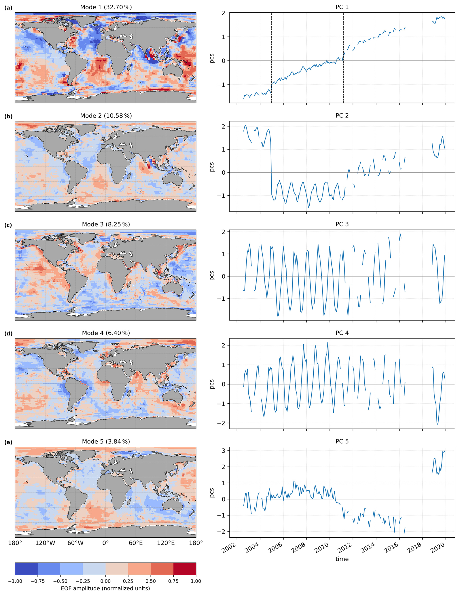
Figure 11 First five empirical orthogonal functions of the GRACE − ECCOv4r5 p_b fields. Time series of principal components (PC) are in units of cm.

Figure 12 (a) Trends (cm yr⁻¹) and (b) standard deviations (cm) of the GRD fields, and (c, d) the percentage of variance in GRACE − ECCOv4r5 p_b fields explained by GRD, based on full fields (c) and detrended fields (d).

Using an EOF decomposition of the GRACE − ECCOv4r5 fields, the first five modes (Fig. 11) account for $\sim \mathrm{2}/\mathrm{3}$ of the total variance, and nearly $\mathrm{1}/\mathrm{3}$ of the variance is associated with mode 1, mostly related to long-term trends in the fields. Mode 1 is clearly affected by the great Sumatra-Andaman and Tohoku earthquakes, with changes in behavior of its principal component evident in 2004 and 2011, but there are strong loadings in other places (e.g., Arctic, North Atlantic, near Antarctica). The Sumatra-Andaman earthquake and to a lesser extent the Tohoku earthquake seem to affect also mode 2, which includes more of the seasonal component that is predominant in modes 3 and 4. More mixed monthly to interannual variability relates to mode 5, with an apparent large change across the GRACE and GRACE-FO gap. Loading patterns in modes 3–5 are mostly basin scale, with enhanced magnitudes near some continental boundaries (e.g., around South America in mode 4).

The long-term trends highlighted by the EOFs in Fig. 11 can be partly due to representation errors associated with geophysical processes of non-oceanographic origin. Earthquakes typically involve large step-like, co-seismic jumps and post-seismic nonlinear temporal behavior (e.g., Han et al., 2013). These signals can be modeled empirically and removed from the GRACE fields, as done for several products recently made available (e.g., Dahle et al., 2025; Bonin et al., 2026). Although not available for the GRACE product employed in this work, such an earthquake correction, based on the model of Han et al. (2013), is currently being developed and is planned for inclusion in the next release of the JPL mascon solutions (David Wiese, personal communication, 2025). Given a focus on p_b and ocean dynamics, future GRACE data constraints might make use of fields that have been corrected for all major earthquake signals.

Other geophysical factors that can contribute to GRACE − ECCOv4r5 fields include GRD effects and glacial isostatic adjustment (GIA; Whitehouse, 2018). Expanding on the treatment of the mean seasonal cycle discussed by Ponte et al. (2024), here we make use of the recent GRD estimates by Landerer and Wiese (2025) to examine their possible effects on GRACE − ECCOv4r5 fields. Trends in GRD fields (Fig. 12a) are relatively large around Greenland and west Antarctica and related to the melting of ice sheets and glaciers. Other GRD variability (Fig. 12b) is also seen around many continental boundaries (e.g., western North America, South America, Southeast Asia), which is mostly related to the seasonal cycle in land hydrology.³ The percentage of variance in GRACE − ECCOv4r5 misfits explained by GRD effects (Fig. 12c), calculated as

$$\begin{array}{}\text{(2)}& \left[\mathrm{1}-{\displaystyle \frac{\mathrm{variance}(\mathrm{GRACE}-\mathrm{ECCOv}\mathrm{4}\mathrm{r}\mathrm{5}-\mathrm{GRD})}{\mathrm{variance}(\mathrm{GRACE}-\mathrm{ECCOv}\mathrm{4}\mathrm{r}\mathrm{5})}}\right]\times \mathrm{100}\mathit{\%},\end{array}$$

is substantial in some of these areas. Differences between results using full versus detrended fields (Fig. 12c and d) indicate the importance of trends in Baffin Bay, eastern subpolar North Atlantic, and the Amundsen/Bellingshausen Sea sectors of coastal Antarctica, where values of percentage variance explained are largest (>50 %). Aside from trends, GRD variability mostly associated with the seasonal hydrological cycle in the Amazon can also explain >50 % of the variance in detrended misfits around South America (Fig. 12d). Similar results apply to other coastal regions like western North America. These latter findings are consistent with those in Ponte et al. (2024).

Unlike GRD effects, GIA is solely related to long-term trends (Whitehouse, 2018). Although such trends are modeled and removed from GRACE fields (Watkins et al., 2015), uncertainties in the models (Caron et al., 2018) can also contribute to differences between ECCOv4r5 and GRACE. Estimates of GIA trend errors by Caron et al. (2018), on the order of 1 mm yr⁻¹ away from the main glaciation regions, are not negligible compared to differences in GRACE, ECCOv4r5 trends in Fig. 4d. Moreover, enhanced GIA errors in parts of the Arctic (Kara, Barents and Beaufort Seas) and in coastal Antarctica (cf. Fig. 3, Caron et al., 2018) coincide with regions of relatively large differences between ECCOv4r5 and GRACE. Although estimated uncertainties in GIA trends can depend on the methodologies used to derive them (e.g., Simon and Riva, 2020), both the pattern and magnitudes of GIA trends and their uncertainties (cf. Fig. 3, Caron et al., 2018) suggest that errors in modeled GIA trends can contribute to the results in Figs. 2 and 4d, particularly near the glaciation regions and in the Arctic.

All the geophysical signals discussed so far can be regarded as representation errors that are best removed from the GRACE observations, if suitable corrections are available. Other representation errors implicit in the ocean model should also be noted. We have already mentioned the effects of intrinsic variability associated with eddies and other nonlinear dynamics, which arise at scales not resolved by the ECCOv4r5 setup but can affect p_b variability at the scales observed by GRACE (Zhao et al., 2021, 2023). The studies of Zhao et al. (2021) and Ponte et al. (2024) are consistent with the influence of intrinsic signals on the enhanced misfits in regions such as the Argentine Basin and the Agulhas Retroflection (Figs. 2a, 5d and 6d). Similar effects may be active in other regions of large eddy activity (e.g., near the Gulf Stream and Kuroshio). Issues of resolution can also lead to representation errors in coastal regions where relatively small-scale boundary geometry and bathymetry features are important. For example, poorly resolved connections between the Gulf of Carpentaria and the Pacifc or Hudson Bay and the Atlantic are likely to hamper the ability to faithfully represent p_b variability in those regions.

6 Summary and concluding remarks

Ocean bottom pressure (p_b) is a key variable for tracking changes in the state of the oceans and climate, but space gravity data from GRACE provides relatively limited resolution in space and time. Ocean models can help fill data gaps but are prone to errors. This study uses the ECCO state estimation framework to assess the impact of data constraints, in particular those provided by both local and global mean GRACE data, on optimizing model-based solutions and determining “best estimates” of p_b fields. Based on comparisons of ECCOv4r5 and ECCOctrl fields (Sect. 3.1), the full data constraints lead to substantial adjustments of local p_b fields. Largest changes occur at polar/subpolar and coastal regions, where p_b variability is also largest. The optimized p_b fields in ECCOv4r5 are mostly closer to the GRACE data, within expected uncertainties. Modifications to the p_b fields occur over all timescales, from monthly to multi-decadal, and tend to have large, basin scales (Sect. 3.2).

The p_b adjustments for periods with GRACE constraints are notably larger than those for periods without GRACE data (Sect. 3.3). Differences in their respective standard deviations of order 1 cm (Fig. 9) are equivalent to changes in the barotropic streamfunction of a few Sverdrups (1 Sv = 10⁶ m³ s⁻¹) over the deep ocean (e.g., Gill and Niller, 1973). Larger differences of a few centimeters in many coastal regions also imply substantial changes in circulation. Our results indicate the importance of GRACE constraints in the ECCO optimizations for determining local p_b variations and associated circulations and extend previous findings by Köhl et al. (2012) and Saynisch et al. (2015), which were inherently limited by the shortness and relatively higher noise of the early GRACE data records. What is more, the novel GRACE constraint on global mean p_b described in this study helps correct freshwater flux errors in the MERRA-2 atmospheric reanalysis, leading to more realistic barystatic sea level estimates in ECCOv4r5 (Sect. 4).

The remaining differences between ECCOv4r5 and GRACE point to potential issues with geophysical (non-oceanographic) signals present in GRACE data used in our study (Sect. 5). Recent derivation of “corrections” for effects of earthquakes and GRD (Landerer and Wiese, 2025; Dahle et al., 2025; Bonin et al., 2026) and continued developments in GIA modeling (Whitehouse, 2018) shall prove crucial in improving the quality of GRACE data for p_b estimation. In addition to GRD, GIA and earthquakes, other geophysical signals of more speculative origin, having to do with deep gravity anomalies associated with core and mantle dynamics, may also play a role in the GRACE − ECCOv4r5 residuals (e.g., Gouranton et al., 2025, and references therein). Such signals are not well understood, however, and thus not ripe for forward modeling as with GRD and GIA.

From a broader geophysical perspective, insofar as ECCOv4r5 yields a valid estimate of p_b variability related to ocean dynamics, the GRACE − ECCOv4r5 fields can serve as a refined estimate of non-oceanographic gravity anomalies, which can then be studied in further detail (e.g., Gouranton et al., 2025). A more advanced possibility would involve the joint estimation of p_b and other geophysical parameters by bringing together models of the different components (solid Earth, hydrology, cryosphere, ocean) and other relevant datasets (e.g., laser altimetry of the ice sheets).

Estimation of “best” p_b fields can also benefit from developments on the modeling and estimation side. Some of our results suggest that GRACE errors used in ECCOv4r5 might have been both underestimated (e.g., in the regions of the large earthquakes) and overestimated (e.g., in the low and mid latitudes). Continuous refinement of GRACE data weights will be needed, as non-oceanographic signals and more generally data noise are removed in future data releases. More advanced data weighing involving non-diagonal covariance terms is also possible, although their estimation is challenging. On the modeling side, increased resolution should help with representation of bathymetric features such as continental slopes and connections to marginal seas (e.g., Bab el-Mandeb, Gibraltar, and Hudson Straits), which are important in modulating p_b variability in such regions. Shallow coastal domains (e.g., Arctic shelves) may also benefit from finer resolution as well as modified parameterizations of bottom friction (future optimizations could include bottom friction parameters as part of the “controls”). Note, however, that higher resolutions that allow realistic eddy fields will present other challenges in estimating large-scale p_b fields, particularly where non-negligible intrinsic p_b variability is expected (Zhao et al., 2021, 2023; Ponte et al., 2024).

Our analyses are based on the ECCO framework, with specific estimation methodogy, model settings, and data products. Storto et al. (2024) highlight the substantial differences in p_b estimates produced by several available data assimilation systems, none of which consider the use of GRACE constraints. Hopefully, this study can stimulate the inclusion of GRACE data in future ocean reanalysis and state estimation efforts and serve as a baseline for exploring the influence of such data on the behavior of p_b and associated circulation fields. The use of dedicated data withholding experiments (e.g., Köhl et al., 2012) would help to further quantify the impact of GRACE data constraints in p_b estimation. Such analyses are relatively easy to implement in an ECCO framework but can be computationally slow and expensive and are left for future study.