High-latitude eddy statistics from SWOT compared with in situ observations

Mesoscale eddies play a key role in the transport of heat, salt, and momentum in the ocean, yet their statistical characterization at high latitudes has remained elusive due to the coarse resolution of conventional satellite altimetry. Here we present a statistical description of the mesoscale eddies in the Labrador Sea at an unprecedented resolution, using observations from the Surface Water and Ocean Topography (SWOT) mission, significantly extending previous estimates derived from lower-resolution altimetry products. We apply an eddy-detection algorithm directly to the native 2 km SWOT swaths, without gridding or assimilation, and validate the detections against in situ measurements from shipboard current profiler data from one cruise in 2024, as well as against a statistically derived shipboard current-profiler-based eddy census. The comparison demonstrates good agreement in eddy size and intensity, confirming SWOT's ability to resolve high-latitude mesoscale structures previously undetectable or distorted in gridded altimetry. The SWOT-derived eddy census based on two full calendar years reveals a predominance of energetic anticyclones (Irminger Rings) in the basin interior and smaller cyclones along the continental slopes, with clear seasonal variability linked to boundary current instability. These findings provide the first observational benchmark for mesoscale activity in the Labrador Sea and illustrate SWOT’s potential to extend eddy statistics to high-latitude and ice-influenced regions, opening the way for a global assessment of mesoscale variability.

1 Introduction

Mesoscale eddies are ubiquitous features of the world ocean, playing a fundamental role in the transport of heat, salt, and nutrients, as well as in the redistribution of momentum and energy across spatial scales (Chelton et al., 2011; Zhang et al., 2014; Dong et al., 2014). Given their widespread influence, detecting and characterizing mesoscale eddies at the global scale has long been a key objective of physical oceanography.

Over the past two decades, global automatic eddy detection has been made possible through the availability of gridded sea level anomaly (SLA) products derived from conventional nadir altimetry (see all literature from Chelton et al., 2007). These datasets have allowed systematic eddy tracking and the construction of global eddy atlases. However, these products are fundamentally limited by their spatial resolution, usually 1/4 or 1/8°, which constrains their ability to resolve eddies smaller than ∼50 km in diameter (Ballarotta et al., 2019). The ability of gridded SLA fields to represent the eddy field has previously been questioned, as they have largely distorted eddy characteristics (Amores et al., 2018). This is linked to the spatio-temporal interpolation during the mapping procedure which compromises the scales to be resolved, and sampling capabilities (Le Traon et al., 1998; Pujol et al., 2016). Validation of such large-scale eddy datasets remains sparse, as direct in situ observations suitable for comparison are rare and spatially limited. Furthermore, a major blind spot persists at high latitudes (>50° N/S), where the first baroclinic Rossby radius of deformation (R_D) is only a few tens of kilometers (de Marez et al., 2025b), well below the resolving capacity of conventional altimetry (Amores et al., 2018).

Yet, mesoscale dynamics at high latitudes play a critical role in shaping water mass transformation and air–sea heat exchange, notably within subpolar gyres and regions of deep convection (Beaird et al., 2016). Eddies mediate restratification after winter convection, influence deep-water formation, and contribute to the variability of boundary currents (Rieck et al., 2019; Du Plessis et al., 2019; Zhang et al., 2022). They are particularly abundant in two dynamical environments: the marginal ice zone (MIZ) and the unstable coastal currents that border subpolar basins. In the MIZ, sea-ice melt generates sharp density gradients that trigger geophysical instabilities and lead to intense eddy formation; these eddies, often organized as dipoles, actively disperse sea-ice floes and contribute to the widening of the ice edge region (Manucharyan and Thompson, 2017; Manucharyan et al., 2022). Their associated heat fluxes also accelerate sea-ice melt by transporting warm, saline waters toward the surface and poleward (Thompson et al., 2014; Si et al., 2023). This results in a positive feedback between eddy activity and sea-ice retreat: the more eddies, the more sea ice melts (Manucharyan and Thompson, 2022). Furthermore, even in the absence of sea-ice, regions located near the MIZ remain dynamically influenced by freshwater input and stratification associated with ice melt (de Marez et al., 2025b). In the boundary currents, mesoscale eddies are frequently generated through barotropic/baroclinic instability and can detach as coherent vortices – such as Irminger Rings from the West Greenland Current (de Jong et al., 2014) – playing a key role in the lateral transport of heat, freshwater, and biogeochemical tracers into the basin interior. However, because of their small spatial scales and the scarcity of in situ observations, the statistical properties of high-latitude eddies remain poorly constrained, leaving a major gap in our understanding of polar and subpolar ocean dynamics.

Here, we take advantage of the unprecedented capabilities of the Surface Water and Ocean Topography (SWOT) wide-swath altimeter to bridge this gap. For the first time, SWOT allows us to resolve and characterize mesoscale eddies at high latitudes with a resolution fine enough to capture the relevant spatial scales. Using SWOT 2 km sea level anomaly swaths, we develop and apply an eddy-detection methodology specifically designed to preserve small-scale variability and to quantify eddy statistics. We focus on the Labrador Sea, where SWOT-derived eddy characteristics can be validated against independent and statistically robust in situ measurements from the shipboard surveys described in Bendinger et al. (2025). This latter study provides a uniquely comprehensive, ship-based census of mesoscale and submesoscale eddies in the central Labrador Sea, offering an ideal reference for assessing SWOT's performance. In parallel, recent work by Jensen et al. (2025) has demonstrated SWOT’s ability to reveal mesoscale features at such high latitudes (in another region, the East Greenland Shelf). While their study focuses on the detailed characterization of SLA snapshots and relies primarily on SST for validation, our approach extends this capability toward a quantitative and statistically grounded assessment of the eddy field at high latitude, supported by a dedicated in situ reference dataset.

This study presents a statistical description of mesoscale eddies at high latitudes in the Labrador Sea, using wide-swath satellite observations, significantly extending previous estimates derived from lower-resolution altimetry products. Section 2 describes the data. Section 3 presents the methodology of the SWOT-based detections and its validation against in situ observations. Section 4 discusses the spatial and temporal variability of eddy characteristics in the Labrador Sea, and Sect. 5 discusses and summarizes the main findings of the study.

2 Data

2.1 SWOT data

We leverage SWOT satellite data (see e.g., Morrow et al., 2019, for some background). We use the latest release (v3.0) of Level-3 SWOT data, namely the SWOT_L3_SSH “Basic” (2 km resolution) product, derived from the L3 SWOT Ka-band Radar Interferometer (KaRIn) Low rate ocean data products provided by NASA/JPL and CNES. The Level-3 processing removes SWOT's systematic errors, and has been extensively validated using other altimeters, numerical models, and in situ data, in the global ocean (Dibarboure et al., 2025). These datasets are produced and freely distributed by the AVISO and DUACS teams as part of the DESMOS Science Team project (AVISO/DUACS, 2023b).

Here, we use the “filtered” Sea Level Anomaly (SLA) variable. The filtering procedure is described in Tréboutte et al. (2023). It is based on a U-Net-based convolutional neural network, trained on simulated North Atlantic data, and shown to outperform classical filtering methods. The method reduces significantly the noise (by a factor of 2), while preserving the balanced part of the signal at spatial scales down to 10 km (Demol et al., 2026). This method allows extraction of most of the balanced signal from the full Sea Surface Height (SSH) field, but it also reduces the overall energy, which can complicate interpretation at small scales where signal levels approach the noise floor (see e.g., Callies and Wu, 2019). This effect primarily impacts the high-wavenumber part of the spectrum, where reduced energy can become comparable to instrumental noise. However, this limitation does not affect our analysis, as we focus on mesoscale structures whose signal amplitude remains well above the noise level (Chelton, 2024). Recent studies have indeed demonstrated SWOT's ability to robustly resolve mesoscale variability that was previously undetected in gridded products (Zhang et al., 2025b, 2024; Verger-Miralles et al., 2025; Du and Jing, 2024; Damerell et al., 2025; Carli et al., 2025; Dibarboure et al., 2025; Zhang et al., 2025a; de Marez et al., 2025b; Archer et al., 2025).

We consider data during the “science phase” (with a 21 d repeat orbit), from cycle #6 to cycle #41, covering the period from 11 November 2023 to 17 November 2025, thus two whole seasonal cycles. We extract SWOT measurement in the Labrador Sea area, which represents 74 SWOT passes in total (see one cycle of measurement in the area of interest in Fig. 1).

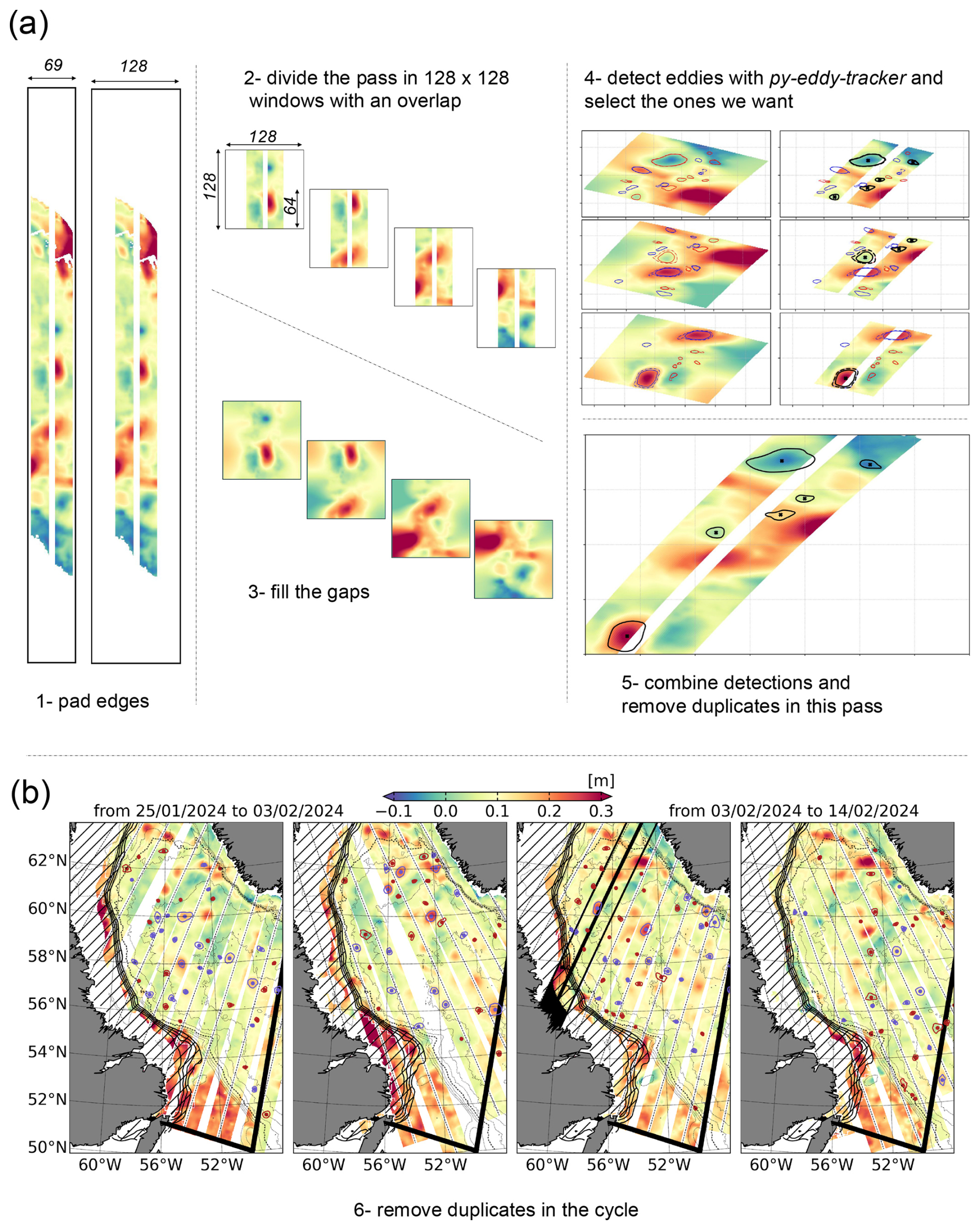
Figure 1 (a) Example of the detection methodology in pass #563, and cycle 10. (b) Mesoscale eddy detection in the Labrador Sea from non-interpolated SWOT data for cycle 10; blue (resp. red) contours (resp. dots) indicate anticyclonic (resp. cyclonic) eddy contours of maximum velocity (resp. centers); thin contours indicate isobaths every 500 m (dotted line highlights isobath 2000 m); thick contours indicate the average sea ice concentration in the period of the map every 10 % (the >10 % area is hatched); the pass #563 shown in panel a is highlighted in the third panel.

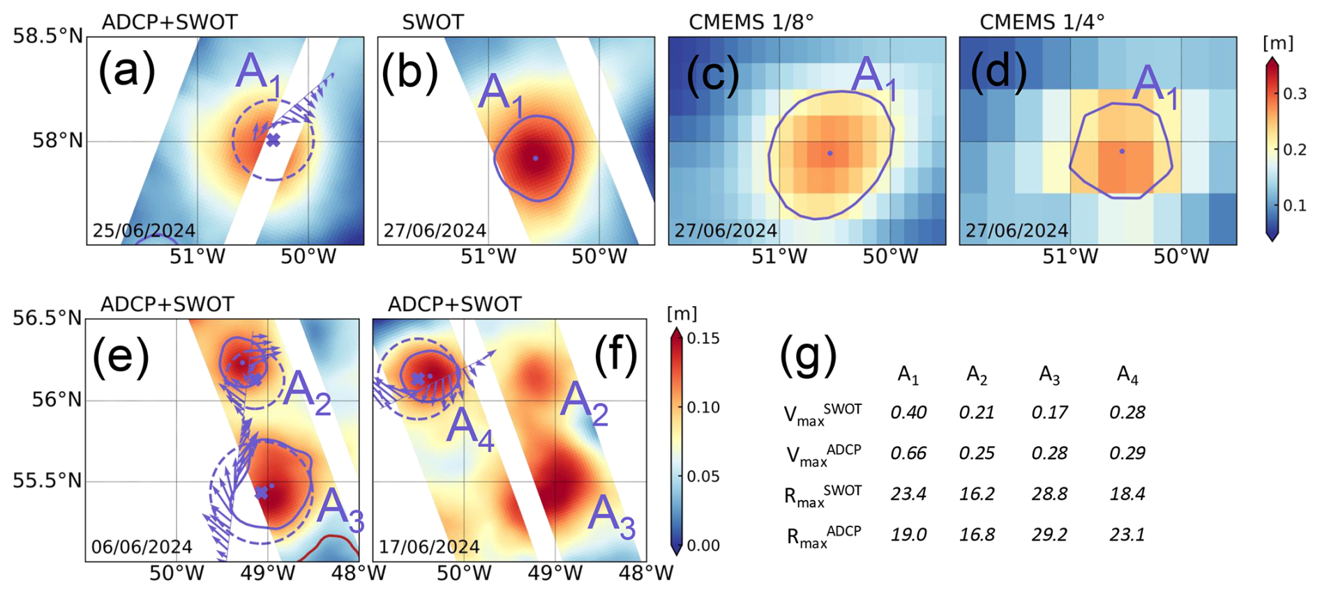
Figure 2 Comparison between eddy detections in SWOT altimetry data, CMEMS data, and the eddy identification method of Bendinger et al. (2025) applied to observations from the 2024 MSM129 cruise in the Labrador Sea, where four eddies were observed. Panels (a), (b), (e) and (f) show the sea level anomaly (SLA) from SWOT, over which detected eddies are mapped. In panels (b), (e) and (f), solid lines indicate the maximum azimuthal velocity contours of SWOT-detected eddies, and dots mark their centers. In panels (a), (e) and (f), crosses indicate the centers of eddies identified during MSM129, with circles marking their radii; arrows show the surface velocity from the SADCP, used for the in situ eddy identification along the ship’s trajectory. Eddies A_1–4 correspond to the four observed structures. Their maximum velocity (in m s⁻¹) and radius (in km) are summarized in panel (g) for both SWOT detections and SADCP identifications. Panels (c) and (d) show the detection of eddy A₁ from CMEMS 1/8 and 1/4° SLA, using py-eddy-tracker.

2.2 SADCP data

We complement the SWOT satellite observations with ship-based velocity measurements obtained from Shipboard Acoustic Doppler Current Profilers (SADCPs). SADCPs provide high-resolution profiles of horizontal current velocity along the ship track by measuring the Doppler shift of acoustic signals reflected by waterborne scatterers. The instruments operated at frequencies between 38 and 150 kHz, providing near-surface velocity estimates at an along-track resolution of roughly 200–300 m. SADCP data collected during MSM129 in June–July 2024 aboard the RV Maria S. Merian is used, with the instrument operating at 75 kHz, and providing near-surface velocity estimates at an along-track resolution of roughly 200–300 m. The data were processed following the same procedure as for MSM74, as detailed in Bendinger et al. (2025). The processed ship-based velocity measurements were then used to fit idealized eddy solutions along the SADCP transects, allowing reconstructions of eddy centers and key dynamical properties (see Bendinger et al., 2025 for methodological details). These reconstructions provide a robust in situ “truth” against which we can directly assess the performance and reliability of the SWOT-based eddy detection, enabling a direct comparison of mesoscale eddy structures between SWOT and MSM129 (Fig. 2). In addition, we compare the statistical results of Bendinger et al. (2025), which are based on SADCP observations from the MSM40, MSM54, and MSM74 cruises and comprise 40 well-resolved eddies with radii of 3–39 km and azimuthal velocities of 7–58 cm s⁻¹, with the SWOT-based statistics, as shown in the histograms in Fig. 3.

Eddy detection statistics from a classical 1/4° satellite altimetry are also used for comparison purpose. The detection was performed by Bendinger et al. (2025) using the AMEDA algorithm (Angular Momentum Eddy Detection and Tracking Algorithm; Le Vu et al., 2018), and is referred to as “CMEMS” for Copernicus Marine Environment Monitoring Service in e.g., Fig. 3b and d. Note that these eddy statistics are only representative of eddies along or close to the ship tracks of MSM40, MSM54, and MSM74 campaigns. Also, note that higher-resolution products such as the DUACS DT2024 1/8° fields are now available and could improve the representation of smaller-scale structures (see e.g., Figs. 2c and d). Nevertheless, we do not expect that increasing the resolution from 1/4 to 1/8° would qualitatively alter the main conclusions presented in Fig. 3b and d.

2.3 Other datasets

We use the sea ice concentration from the OSI SAF dataset (CMEMS, 2026), and the ETOPO Global Relief Model dataset (NOAA National Centers for Environmental Information, 2022) to assess respectively the sea ice concentration, and the depth at each eddy location.

3 Eddy detection from non-interpolated SWOT data

3.1 The methodology

Each SWOT pass consists of two adjacent swaths, each approximately 50 km wide, resulting in a combined swath width of about 120 km. These swaths are separated by a nadir gap of approximately 20 km, where no KaRIn measurements are collected. See for example the “raw” pass #563 of cycle #10 in the top left of Fig. 1. The swaths are oriented along the satellite's ground track, providing detailed across-track coverage. Within each pass, the measurement grid is composed of 69 across-track pixels, and N along-track pixels, with each pixel representing a 2 km by 2 km area on the Earth's surface. Measurement gaps can occur within the swaths due to various factors, including rain cells which can attenuate the radar signal and lead to missing data in certain regions, or sea ice for example.

We apply an eddy-detection procedure directly on the 2 km resolution swath product of SWOT, without performing any subsequent gridded assimilation, in contrast to classical gridded altimetric product based eddy detection approaches, that now include SWOT measurements (see e.g., Gómez-Navarro et al., 2025, who used MIOST, the Experimental multimission gridded L4 sea level heights and velocities with SWOT KaRIn data). Working in the native swath geometry maximizes our ability to identify small‐scale features that might otherwise be lost in the smoothing and gridding stages of standard products. Additionally, the mesoscale eddies in our high-latitude study region are smaller than this swath width, hence an eddy can typically wholly be contained within a single swath pass – enabling reliable detection and sizing. The procedure is as follows (see also Fig. 1 for an example):

We use the native 2 km resolution SWOT swaths, which are 69 pixels wide in the across-track direction. To enable efficient processing, each swath is first extended by padding its lateral edges with NaNs values (step #1 in Fig. 1a), leading to 128-pixel wide swaths. The padded swath is then subdivided into overlapping 128×128 pixel windows, with an overlap of 64 pixels between adjacent tiles (step #2 in Fig. 1a). Each tile therefore contains the original data along with regions of missing values (NaNs), including the nadir gap. These gaps are then filled independently within each tile using a biharmonic inpainting method, resulting in complete 128×128 SLA images (step #3 in Fig. 1a). Specifically, we use the inpaint_biharmonic function from the skimage.restoration Python module, which reconstructs missing values by solving the biharmonic equation (∇⁴u=0) inside the gaps. Note that the tiling procedure is needed to make the inpainting method computationally tractable.

This inpainting method ensures a smooth interpolation by minimizing the Laplacian of the interpolated field, producing a physically consistent and continuous surface that preserves the mesoscale eddies structure and allows closed contours to form even across the gap between the two swaths. Note that the gap-filling methodology may lead to misdetections, particularly for larger eddies, as these structures more frequently intersect gap regions; however, eddies with radii ≲15 km remain largely constrained by observations, so the inpainting does not significantly bias the statistics in the size range considered here (see Appendix A for details).

Eddies are then identified in each sub-image using the py-eddy-tracker package (Mason et al., 2014). We relied on this eddy detection method with standard parameter choices, ensuring robustness, reproducibility, and consistency with existing studies. Note that sensitivity to the shape error parameter used in py-eddy-tracker was conducted, and it was shown to not bias the statistical properties of the eddy population, we therefore used the value of 85 % to maximize the number of detections.

Eddies are assumed to be predominantly geostrophic, and although ageostrophic (cyclostrophic) corrections may become relevant for the most intense structures (e.g., Ioannou et al., 2019), they are neglected here as a first-order approximation, following standard practice for mesoscale structures in altimetric data.

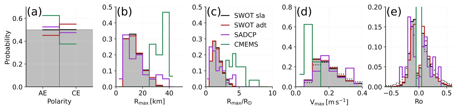
Figure 3 Probability distribution of eddy statistics detected by SWOT using SLA (gray bars, solid black lines) or ADT (red lines), in comparison with ADCP (purple) and CMEMS (green). (a) Polarity of detected eddies, expressed as the proportion of anticyclonic (AE) and cyclonic (CE) structures. (b) Distribution of radius of maximum azimuthal velocity R_max. (c) Distribution of R_max normalized by the first baroclinic deformation radius R_D. (d) Distribution of maximum azimuthal velocity V_max. (e) Distribution of the Rossby number $Ro=\frac{V_{\max }}{f_{\mathrm{0}}{R}_{\max }}$ of detected eddies; for CMEMS, the probability reaches 0.6 for $-\mathrm{0.05}<Ro<\mathrm{0}$ and 0.4 for $\mathrm{0}<Ro<\mathrm{0.05}$. In panels (c) and (d), dotted lines are distributions including all detections prior to depth filtering (i.e., <2000 including eddies on shelves).

We sort detected eddies using a set of predefined criteria to ensure robustness (step #4 in Fig. 1a). First, a maximum of 40 % of the eddy contour (defined by the region of maximum azimuthal velocity) is allowed to overlap with gaps in the SLA field, preventing spurious features generated by the inpainting procedure. This condition is suppressed when the eddy center lies near the middle of the pass (in the gap between swaths) and a tolerance of 60 % of gaps is then allowed. Finally, only eddies exceeding a minimum radius of 5 km and a minimum amplitude of 0.01 m are retained. We chose relatively conservative thresholds to ensure robust detection of balanced structures in the filtered SWOT SSH fields, minimizing spurious detections due to noise or residual unbalanced motions; while this choice may exclude the weakest eddies, it does not significantly affect the statistical distributions and ensures the reliability of the analysis. Note that sensitivity tests to all these parameters were performed to choose their values – low variability of probability distributions was obtained from these sensitivity tests.

The remaining eddy arrays from all sub-images are merged, with duplicates in the overlapping regions removed, providing a complete set of eddy detections for each SWOT pass (step #5 in Fig. 1a).

Finally, for each cycle, duplicates are removed by identifying eddies whose centers are separated by a distance shorter than their radius of maximum velocity (hereafter radius or R_max for conciseness) and a distance threshold of 10 km. This threshold corresponds to the typical displacement of an eddy advected by Rossby wave propagation over one SWOT repeat cycle. When duplicates are identified, one of the two eddies is retained without preferential selection – specifically, the first occurrence in the sequence of passes is kept. This ensures that the procedure does not introduce systematic biases in eddy characteristics. As an example, the anticyclonic eddy located at 60° N, 54° W (left panel in Fig. 1b) is detected in multiple passes during the cycle but retained only once after merging.

Eddies detected at a position where sea ice concentration is larger than 15 % are removed. Further, for the comparison with ship-derived eddy characteristics (see Sects. 2.2 and 3.2), we only consider eddy detections at depths larger than 2000 m to solely focus on eddies in the central Labrador Sea, similarly to Bendinger et al. (2025).

This methodology therefore gives for each SWOT cycle all detected eddies in the area of interest (see Fig. 1b). It is important to note that an eddy may be re-detected in successive cycles; therefore, this methodology does not provide the absolute number of eddies, but rather a detection probability per cycle. The method may also detect a few submesoscale vortices where R_D is large, but these cases fall near the mesoscale–submesoscale transition ($R/R_{\mathrm{D}}\sim \mathrm{1}$; see Fig. 3). We therefore treat all detections as mesoscale eddies in this study.

Detection consistency using this methodology was qualitatively assessed using SWOT Cal/Val data in the Labrador Sea (notably pass #20). The analysis of consecutive daily detections shows overall good temporal consistency despite occasional, expected misdetections due to evolving structures and sampling variability. No quantitative metric was applied at this stage.

Detection was performed using both Sea Level Anomaly (SLA) and Absolute Dynamic Topography (ADT) fields. In the Labrador Sea, the resulting eddy statistics and validation against in situ observations are very similar for the two approaches. In the main manuscript, we nevertheless present the SLA-based detections, as most recent studies investigating eddies from SWOT observations have relied on SLA fields (e.g., Zhang et al., 2025a; Zhu et al., 2026; Han et al., 2026; Fu et al., 2026). For comparison purposes, ADT-based results are additionally shown in Fig. 3 and in Appendix B. A detailed assessment of the impact of the Mean Dynamic Topography (MDT) provided in SWOT product and of the relative performance of SLA versus ADT for SWOT-based eddy detection is beyond the scope of the present study and is left for future work.

3.2 Validation of the method using in situ data

Validating the eddy detection method requires comparing the eddy characteristics obtained from SWOT data with independent in situ observations of eddies in the same region: this comparison must rely on another source of measurement, with eddy statistics derived from an alternative detection approach. However, establishing a suitable ground truth is not straightforward. On one hand, classical gridded altimetry products cannot serve as a reference, since their coarse resolution and interpolation algorithm prevent them from resolving mesoscale eddies in high-latitude regions (Amores et al., 2018; Bendinger et al., 2025). On the other hand, one could consider using eddies detected from high-resolution numerical simulations or reanalyses, either directly on their native grid or by simulating SWOT-like tracks and applying the same detection algorithm. Yet, such an approach would implicitly assume that the model perfectly represents the mesoscale dynamics of the region – an assumption that has not itself been validated, leading to a circular argument.

During the MSM129 cruise conducted in spring 2024 in the Labrador Sea, four anticyclonic mesoscale eddies (hereafter A_1–4) were sampled with the SADCP. The specific tracks crossing the eddies, as well as their associated surface velocity fields (averaged between 22 and 102 m depth), are shown in Fig. 2a, e and f. We take advantage of the method developed by Bendinger et al. (2025) and applied it to this specific dataset, from which the main dynamical properties of the eddies are retrieved to validate the outcome of our SWOT-eddy detection method. The findings are summarized in the table in Fig. 2g.

All four eddies were successfully captured in coincident SWOT passes and detected by our SWOT-based eddy detection method. The eddies identified in SWOT exhibit radii and maximum azimuthal velocities that are in good agreement with those measured during the MSM129 cruise. It is important to note that the SWOT detections and the in situ observations were not made at the same time. For instance, A₁ was observed in situ on 24 June 2024, while its SWOT counterpart was detected on 27 June 2024 (it was also identified on 25 June and 6 July but duplicate detections across cycles were automatically removed; see Fig. 2a–c). The slight reduction in velocity amplitude seen in the SWOT data can be attributed to the instrument's spatial smoothing, which tends to dampen kinetic energy. Also, SWOT altimetry measures an integrated quantity, which tends to be weaker than directly measured surface velocity from SADCP directly. Nevertheless, the close spatial coincidence between eddy centers and contours identified by the two independent approaches, together with their comparable dynamical characteristics, confirms the robustness and reliability of our detection algorithm when applied to the native 2 km SWOT swath data. Note that given the limited number of colocated cases, this agreement should be interpreted qualitatively. Also, note that this in situ validation is based solely on anticyclonic cases; cyclonic eddy properties are validated statistically in the following.

For comparison with standard gridded altimetry, we extracted SLA from the CMEMS 1/4 and 1/8° products on the same date as the SWOT observation of A₁, and applied the same py-eddy-tracker detection parameters (see Fig. 2c and d). This yields velocity for A₁ of V_max=0.29 m s⁻¹ in both datasets, and radii of R_max=33.4 and 25.6 km for the 1/8 and 1/4° products, respectively. This example clearly illustrates the improved effective resolution of SWOT compared to conventional altimetry.

To assess the robustness of our detection method at the statistical level, we use the comprehensive in situ dataset published by Bendinger et al. (2025), which provides a unique reference for eddy statistics in the Labrador Sea. Using their in situ methodology, a large number of mesoscale and submesoscale eddies were identified and characterized, allowing the construction of histograms of the main eddy dynamical properties – including radius, maximum azimuthal velocity, and Rossby number. This dataset thus represents an unprecedented “ground truth” for the eddy field in this high-latitude region, against which we can directly compare the SWOT-based results. The distributions obtained from SWOT (SLA- or ADT-based) detections show remarkable agreement with the in situ statistics, both in terms of typical eddy scales and dynamical intensity, see Fig. 3. When including eddies detected above depth < 2000 m, we find an increased number of small-radius eddies, consistent with the reduced Rossby deformation radius on the continental shelf, but reaching the limitations of SWOT capabilities. Quantitatively, SADCP eddies have a radius between 3 an 39 km (mean 15 km, std 9 km), and azimuthal velocity between 7 and 58 cm s⁻¹ (mean 26 cm s⁻¹, std 13 cm s⁻¹); this compares favorably with SWOT eddies, with radius between 5 and 39 km (mean 14 km, std 6 km), and azimuthal velocity between 5 and 89 cm s⁻¹ (mean 20 cm s⁻¹, std 10 cm s⁻¹). In contrast, the eddy statistics derived from CMEMS gridded altimetry display much larger radii and weaker velocities, reflecting the well-known smoothing and scale limitations of mapped altimetry products at these latitudes; CMEMS eddies have a radius between 25 an 68 km (mean 42 km, std 11 km), and azimuthal velocity between 3 and 12 cm s⁻¹ (mean 8 cm s⁻¹, std 3 cm s⁻¹)

Note that using the recently released v3.0 of SWOT data instead of v2.0.1 improves eddy detection, in particular by (1) reducing the number of spurious small eddies and (2) rebalancing the number of cyclonic and anticyclonic detections (with more cyclones than anticyclones in v2 and approximately equal proportions in v3). This improvement likely results from enhanced noise filtering, i.e., an improved version of the filtered SLA product, and the adoption of the new Mean Sea Surface which significantly reduces the imprint of geodetic structures in the resulting SSH data. A detailed assessment of differences between versions is beyond the scope of this study.

With the in situ validation confirming the reliability and robustness of our detection approach, we can confidently apply it and analyze eddies detected using SWOT in the Labrador Sea. In the following section, we examine the eddy field observed in the Labrador Sea throughout 2024–2025, focusing on the spatial distribution and dynamical characteristics of the detected eddies. This provides a spatial statistical description of the regional mesoscale activity at such high latitude at an unprecedented resolution, significantly extending previous estimates derived from lower-resolution altimetry products.

4 Eddy characteristics in the Labrador Sea during years 2024–2025

The spatial distribution and dynamical characteristics of eddies detected in the Labrador Sea during 2024-2025 are shown in Fig. 4. Anticyclonic eddies (AEs, Fig. 4a–d) are widespread across the basin. They are detected both along the continental slopes and within the deep interior. Their distribution is relatively homogeneous in the central and western Labrador Sea, with enhanced activity near the 3000–3500 m isobaths where mesoscale instabilities of the boundary currents are expected. In contrast, cyclonic eddies (CEs, Fig. 4e–h) are more frequently observed along the continental slopes, particularly in regions influenced by the West Greenland and Labrador Currents, where intense shear and topographic steering promote cyclonic vorticity generation (Chanut et al., 2008; Thomsen et al., 2014; Pacini and Pickart, 2022). This pattern is also found in Fu et al. (2025): they also detected cyclonic eddies in the eastern Labrador Sea from conventional altimetry.

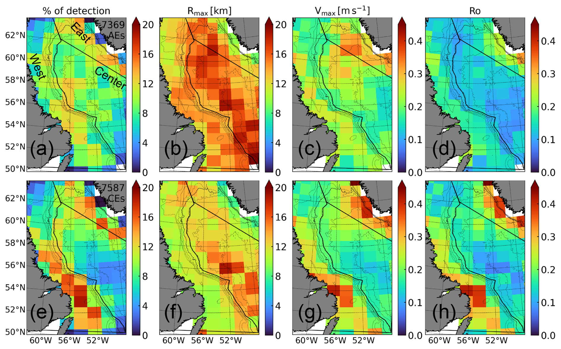
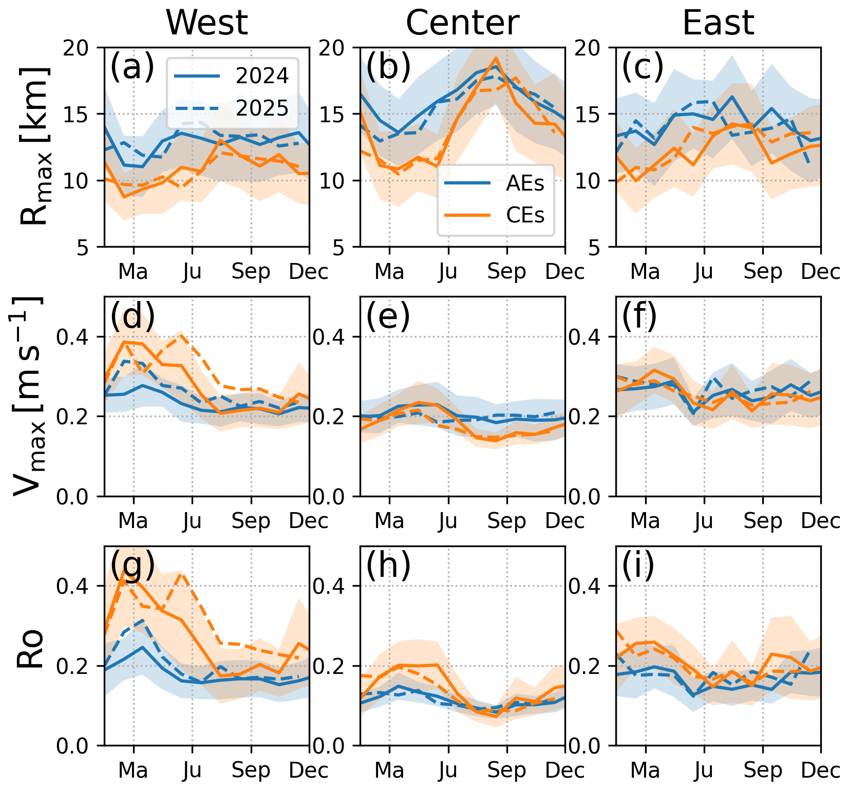
Figure 4 a) Number of detected anticyclonic eddies (AEs) in ${\mathrm{2}}^{\circ }\times {\mathrm{1}}^{\circ }$ boxes during years 2024-2025; each eddy is unique within the cycle it is detected in, but can be re-detected the next cycle as no tracking is performed. b,c,d) Bin-averaged radius of maximum velocity R_max, maximum velocity V_max, and Rossby number Ro of detected AEs. e,f,g,h) Same as panels a,b,c,d but for cyclonic eddies (CEs). Black solid lines indicate the delimitation of areas for the computation of timeseries shown in Fig. 5. Same isobaths as in Fig. 1b are shown.

The observed AE/CE asymmetry likely reflects the greater propagation range of anticyclones. AEs are less susceptible to steering by background currents and less prone to instability-driven decay (Polvani et al., 1994; Arai and Yamagata, 1994; Koszalka et al., 2009; Roullet and Klein, 2010), enabling them to travel farther into the basin interior compared to the more rapidly disrupted CEs.

Eddies exhibit radii of maximum velocity (R_max) ranging between 5 and 34 km, with an average (standard deviation) value of 15(6) km for AEs, and 11(5) km for CEs. The prevalence of large, energetic AEs in the basin interior is consistent with the presence of Irminger Rings (de Jong et al., 2014), which detach from the boundary current system and propagate westward into the convective region. Along the continental slopes, both cyclonic and anticyclonic eddies exhibit higher maximum velocities and elevated Rossby numbers. The enhanced intensity near the slopes likely reflects both active generation processes and stronger strain and frictional interactions with the underlying topography. In these regions, the flow can locally depart from geostrophic balance (Ro∼1), challenging the assumptions made in our methodology.

The delineated boxes in Fig. 4 (black contours) show the sub-regions used to compute the time series of eddy occurrence and mean properties shown in Fig. 5.

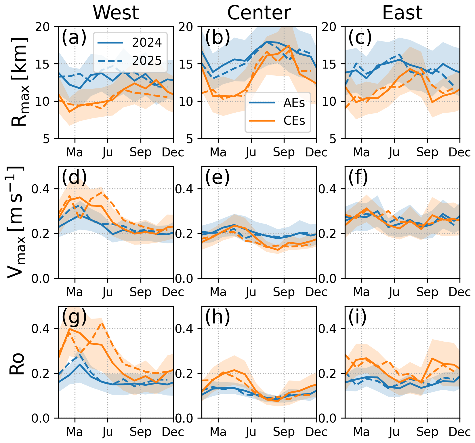
Figure 5 (a–c) Monthly-averaged R_max in the West, Center, and East areas, respectively, for AEs (blue) and CEs (orange) during year 2024 (solid) and 2025 (dashed); areas are defined in Fig. 4; envelopes show the standard deviation. (d–f) Same as panels (a)–(c) but for V_max. (g–i) Same as panels (a)–(c) but for Ro.

In the western area, both eddy types exhibit fairly constant radii of maximum velocity R_max∼10 km, but with noticeably higher velocities (V_max∼0.3–0.4 m s⁻¹) and Rossby numbers (Ro∼0.3) in late winter and spring. This period coincides with the peak of baroclinic instability due to a deepen mixed-layer, which favors the generation of energetic boundary eddies (with slightly smaller R_max).

In the central Labrador Sea, R_max and V_max for AEs increase markedly from spring to early autumn, reaching values near 18–20 km and 0.3 m s⁻¹, respectively. This seasonal strengthening reflects the westward propagation and growth of Irminger Rings as they move into the convective basin, leading to eddy-induced re-stratification after winter deep mixing. Cyclonic eddies, by contrast, remain weaker and smaller throughout the year, consistent with their local generation by shear and topographic interactions.

In the eastern area, eddy properties show larger variability and weaker seasonality. Both AE and CE radii remain around 10–15 km, while velocities seldom exceed 0.25 m s⁻¹. This pattern likely reflects the dominance of small, topographically trapped vortices and the limited mesoscale energy input in the eastern basin.

Overall, throughout 2024–2025, clear regional and temporal contrasts emerge between AEs and CEs. The time series reveal a pronounced seasonal cycle of mesoscale activity: eddies are more energetic during late winter–spring, when baroclinic instability and boundary current variability peak there (see Rieck et al., 2019), and weaken toward autumn, following the re-stratification. The evolution of AE properties in particular highlights the continuous formation, detachment, and westward spreading of Irminger Rings across the Labrador Sea – a process now observed synoptically for the first time with SWOT.

5 Discussion

In the last two decades, a broad range of eddy types have been identified in the Labrador Sea: Irminger Rings, convective lenses, and boundary current eddies, that feature radii in the range of 5–35 km. These observations mostly relied on mooring observations (e.g., Lilly and Rhines, 2002), conventional altimetry (Fu et al., 2025), numerical models (Rieck et al., 2019) or sparse hydrographic sections, which limited the ability to assess eddy statistics or their variability. Here, we provide the first statistically robust description of mesoscale eddies (in the 5–35 km radius range) in the Labrador Sea derived solely from satellite observations. Our SWOT-based detection offers a continuous and quantitative view of the mesoscale field, resolving structures that conventional gridded altimetry could not capture.

The observed eddy characteristics are consistent with previous regional studies describing the prevalence of anticyclonic Irminger Rings and the smaller, topographically constrained cyclones along the continental slopes (de Jong et al., 2014; Pacini and Pickart, 2022). SWOT reveals their full spatial extent and intensity, showing that the mesoscale field is more energetic and heterogeneous than inferred from existing products. By resolving eddies down to scales of a few kilometers, SWOT bridges the gap between in situ observations and large-scale altimetric analyses, offering a new framework to evaluate eddy–convection coupling and boundary current instabilities in subpolar regions. The strong consistency between SWOT and in situ eddy properties validates the approach and provides an observational benchmark for future modelling and reanalysis efforts.

Beyond the Labrador Sea, these results highlight SWOT's transformative potential for observing mesoscale and submesoscale dynamics in high-latitude and coastal environments. Its fine spatial resolution and direct swath observations overcome the scale limitations of conventional altimetry, allowing the detection of eddies of size comparable to the local Rossby radius of deformation with reliable estimates of radius, velocity, and amplitude.

These findings set the stage for the construction of global SWOT-based eddy climatologies, extending into subpolar and seasonally ice covered zones where altimetric data were previously unusable. The Labrador Sea serves as a prototype of such regions, combining strong boundary current variability, deep convection, and seasonal sea-ice influence. Ultimately, SWOT provides a means to quantify how mesoscale turbulence contributes to poleward heat transport and sea-ice variability – a key component of ocean–climate feedbacks.

Appendix A: Gap-filling methodology validation insights from high resolution realistic simulation

To assess the impact of the gap-filling procedure on eddy detection, we conducted a controlled experiment using high-resolution numerical simulations, allowing direct comparison between fully resolved fields and their inpainted SWOT-like degraded counterparts.

We use outputs from a realistic numerical simulation conducted as part of the GIGATL set of Atlantic Ocean simulations (Gula et al., 2021), using the Coastal and Regional Ocean COmmunity model (CROCO), a version of the ROMS model (Shchepetkin and McWilliams, 2005). Specifically, we use one year of the GIGATL1 version with a horizontal resolution of 1 km and 100 terrain-following levels, which allows resolution of mesoscale dynamics in the subpolar Atlantic. We refer the reader to Sect. 2.2 of de Marez et al. (2025a) for a full description of the model setup. We considered simulation outputs in the Labrador Sea.

We use the GIGATL1 SSH field, interpolated onto a 2 km grid to match the effective resolution of SWOT observations. From this interpolated field, we extracted an N×128 domain (see Fig. A1b), which we refer to as the truth field.

We then constructed synthetic SWOT-like swaths by introducing gaps corresponding to the nadir region and the swath edges (see Fig. A1b). This reproduces the exact data geometry encountered in real SWOT observations, with the same grid and missing-data structure as those used in our detection method.

We then applied the same method as presented in Fig. 1: the fields were decomposed into square domains of size 128×128 pixels, and the gaps were filled using the biharmonic inpainting procedure, yielding what we refer to as the SWOT-like fields (see Fig. A1c). This step ensures that the validation framework is fully consistent with the processing applied to the observations in our study.

Eddy detection was then applied independently, to both the truth and the SWOT-like SSH fields, using identical detection parameters. This allows a direct comparison of eddy detection and associated properties between the original and reconstructed datasets (see Fig. A1d). This procedure was repeated on a weekly basis over one year, providing a statistically robust assessment of the impact of the inpainting step on eddy detection.

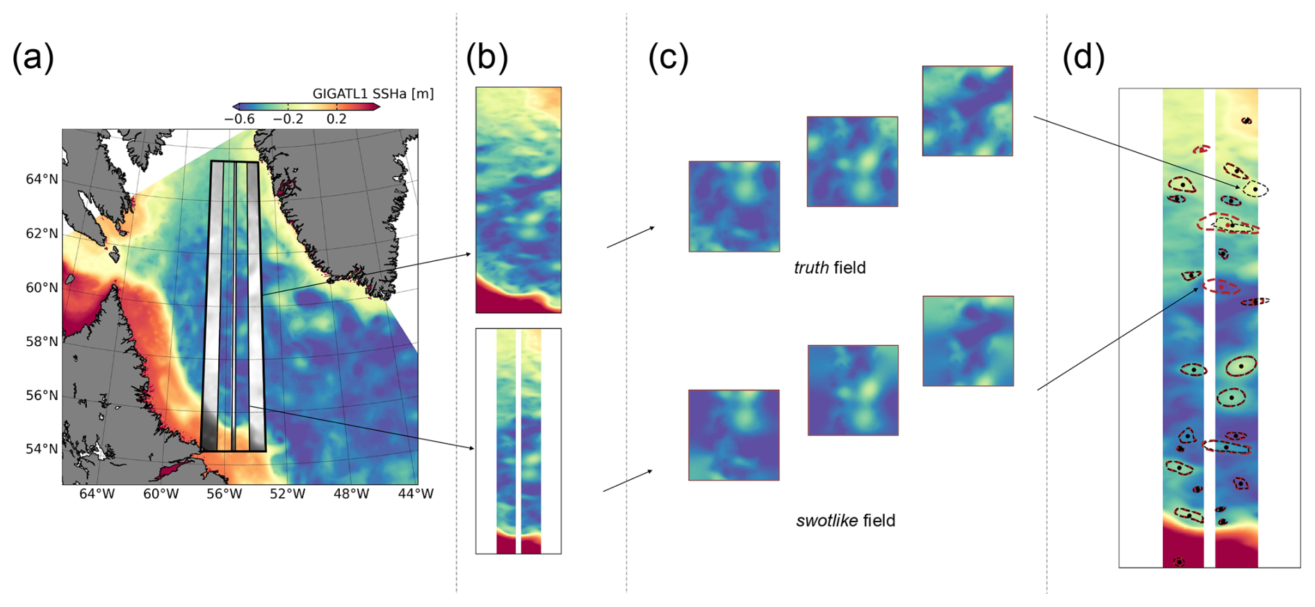
Figure A1 (a) SSH snapshot in the GIGATL1 simulation; the extracted SWOT-like domain is delimited by the thick black lines. (b) Truth and “gapped” SSH field. (c) Truth and SWOT-like SSH fields used for the detection inter-comparison after decomposition into square domain and gap-filling, following the method described in Sect. 3.1. (d) Comparison between eddy centers and contours for detection using either truth (black) or SWOT-like (red) fields.

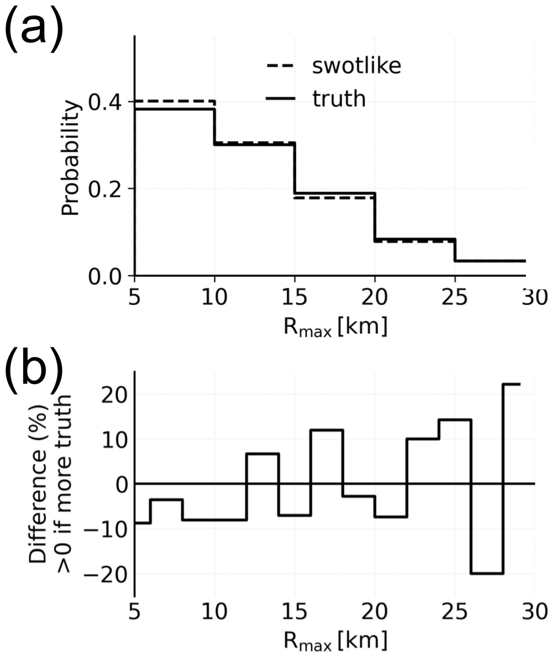
Figure A2 (a) Distribution of radius of maximum azimuthal velocity R_max for eddies detected in truth or SWOT-like SSH fields. (b) Difference (in percentage) of misdetection between the truth or SWOT-like SSH fields as a function of detected eddy radii.

The distributions of eddy amplitude and radius obtained from the truth and swotlike datasets are similar (see Fig. A2a). The misdetection rate on individual passes is ∼5 % over individual passes (∼2 misdetections per pass). Therefore, over annual sampling, the statistical distributions of eddy properties are not significantly altered by the inpainting procedure.

A trend nevertheless appears: discrepancies (difference of the number of detected eddies using the two arrays) increase for eddy radii R_max>20 km (see Fig. A2b). This behavior is physically expected. Large eddies have a broad spatial imprint and therefore intersect the gapped regions more frequently than small eddies, making their reconstruction more sensitive to the inpainting. In contrast, eddies with radii smaller than ∼15 km (i.e., diameters smaller than approximately half the swath width) remain mostly constrained by observed data and are only weakly affected by the extrapolation.

Therefore, the biharmonic inpainting does not significantly bias the eddy statistics in the size range primarily analyzed in this study. The method is robust for eddies whose characteristic scale is smaller than half the swath width, 𝒪(15 km), which corresponds precisely to the population of eddies that SWOT allows us to observe and that are the focus of this paper.

Future work could explore alternative gap-filling strategies, including more advanced approaches such as variational methods or data-driven techniques (e.g., U-Net-based reconstructions), which may further improve the representation of eddies with radii larger than 20 km, or more complex structures. However, the present results demonstrate that a simple, physically constrained inpainting method is sufficient to ensure robust eddy detection at the mesoscale.

Appendix B: Eddy characteristics from detection using ADT

As stated in the manuscript, eddy detection was performed using both SLA and ADT fields. Figures 4 and 5 in the main text correspond to the SLA-based detection. For comparison purposes, we show below the equivalent results obtained using ADT-based detection. Overall, the spatial distributions, eddy statistics, and validation against in situ observations remain very similar between the two approaches. Differences primarily affected the smallest eddies and regions close to energetic boundary currents, where more cyclonic than anticyclonic eddies were detected from the ADT than from the SLA, yielding the polarity asymmetry seen in Fig. 3a for ADT-based detection.

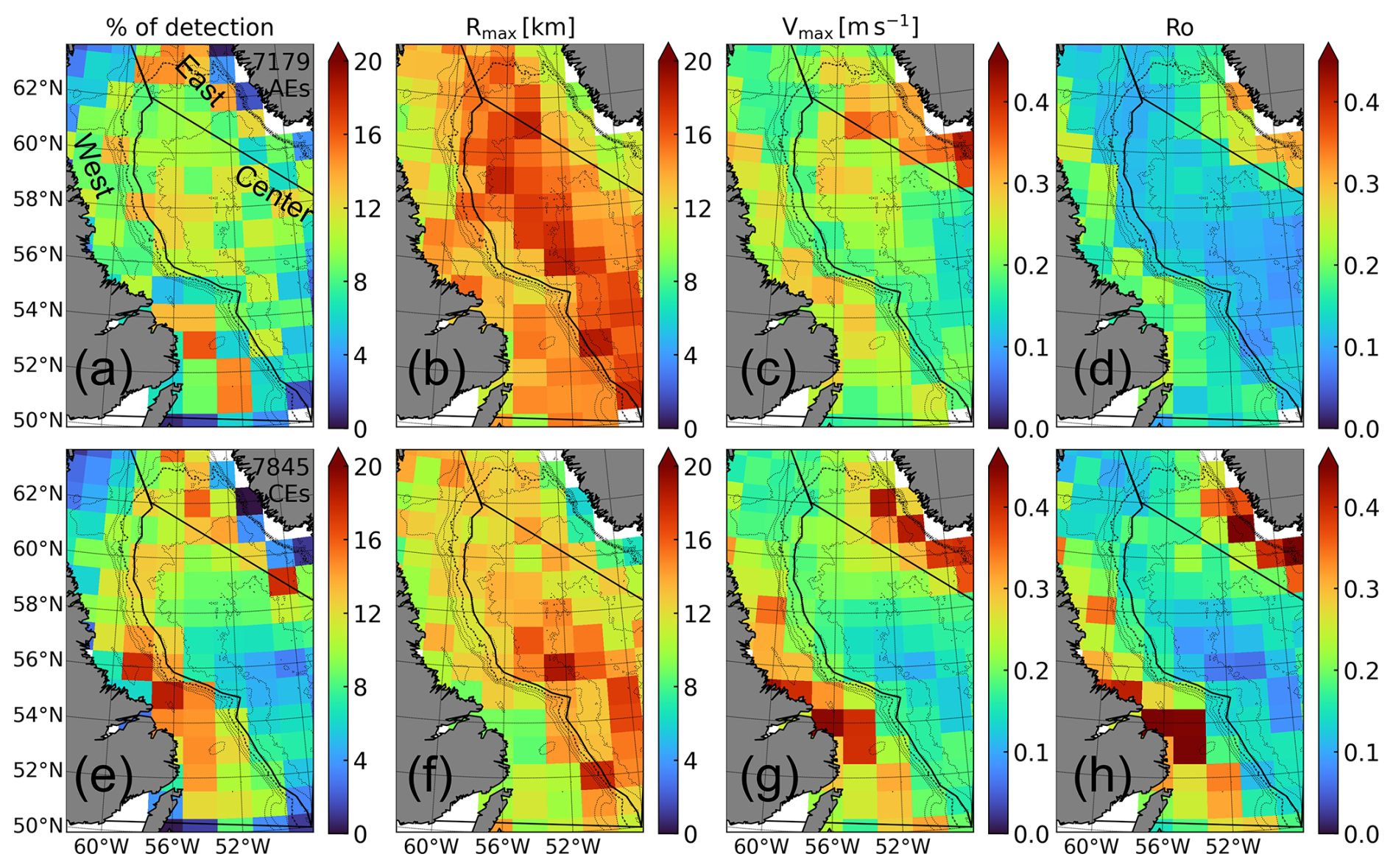
Figure B1 Same as Fig. 4 but using ADT for eddy detection.

Figure B2 Same as Fig. 5 but using ADT for eddy detection.