Process-based modelling of nonharmonic internal tides using adjoint, statistical, and stochastic approaches – Part 1: Statistical model and analysis of observational data

A substantial fraction of internal tides cannot be explained by (deterministic) harmonic analysis. The remaining nonharmonic part is considered to be caused by random oceanic variability, which modulates wave amplitudes and phases. The statistical aspects of this stochastic process have not been analysed in detail, although statistical models for similar situations are available in other fields of physics and engineering. This paper aims to develop a statistical model of the nonharmonic, incoherent (or nonstationary) component of internal tides observed at a fixed location and to check the model's applicability using observations. The model shows that the envelope-amplitude distribution approaches a universal form given by a generalization of the Rayleigh distribution, when waves with non-uniformly and non-identically distributed amplitudes and phases from many independent sources are superimposed. Mooring observations on the Australian North West Shelf show the applicability of the generalized Rayleigh distribution to nonharmonic vertical-mode-one to mode-four internal tides in the diurnal, semidiurnal, and quarter-diurnal frequency bands, provided that the power spectra show the corresponding tidal peaks clearly. These results demonstrate the importance of viewing nonharmonic internal tides as the superposition of many random waves. The proposed distribution can be used for many purposes in the future, such as investigating the statistical relationship between random internal-tide amplitude and the occurrence of nonlinear internal waves, as well as assessing the risk of infrequent strong waves for offshore operations. The proposed statistical model also provides the basis for investigating processes and parameters controlling nonharmonic internal-tide variance in Part 2.

1 Introduction

A substantial fraction of internal tides cannot be explained by harmonic analysis (based on the superposition of sinusoids at tidal frequencies with constant amplitudes and phases). The remaining nonharmonic component is considered to be caused by the random variability of stratification and background currents, which modulate the amplitudes and phases of remotely generated internal tides. In other fields of physics and engineering, statistical models for similar situations – the superposition of waves with constant frequency modulated by a random medium – have been developed. However, the previous studies of nonharmonic, incoherent, or nonstationary internal tides have focused on the temporal aspects of the stochastic process, and the probabilistic or statistical aspects have not been considered in detail. This paper develops a statistical model of nonharmonic internal tides observed at a fixed location by adapting previous statistical models in other fields and then checks the model's applicability to nonharmonic vertical-mode-one to mode-four internal tides in the diurnal, semidiurnal, and quarter-diurnal frequency bands on a continental shelf.

Internal tides are internal waves with tidal frequencies, primarily in the diurnal (≈24 h period) and semidiurnal (≈12 h period) bands. They have different vertical structures, or modes, and lower modes have larger propagation speeds and usually larger energies. (The internal-tide modes are referred to as “baroclinic” modes to distinguish them from the usual tides, or the “barotropic” mode. It is customary to count the first baroclinic mode as vertical mode one, or VM1.) Internal tides are generated by the interaction of tidal currents with topographic slopes, which implies their coherence with the tide-generating forces at the generation sites. However, they gradually become incoherent (or non-phase-locked) as they propagate away from the generation sites (e.g. Rainville and Pinkel, 2006; Buijsman et al., 2017; Alford et al., 2019). This process is considered to be caused primarily by phase modulation through the variability of the wave propagation speed (Park and Watts, 2006; Rainville and Pinkel, 2006), which is in turn caused by temporally and spatially varying pycnocline heaving and advection (Zaron and Egbert, 2014; Buijsman et al., 2017). Higher modes are more susceptible to this phase modulation because their lower propagation speeds increase the relative importance of background currents (Rainville and Pinkel, 2006; Zaron and Egbert, 2014). Although the variability of internal-tide generation can be substantial (Kerry et al., 2016), the amplitude modulation is overall considered to be less important than the phase modulation (Colosi and Munk, 2006; Zaron and Egbert, 2014). However, the generation variability could be more important for higher modes and quarter-diurnal (≈6 h period) internal tides on continental shelves because they can be excited directly by the topographic conversion and nonlinear interaction of incoherent VM1 internal tides, respectively.

Several terms are used to refer to internal tides not explained by harmonic analysis, including nonstationary internal tides (Ray and Zaron, 2011; Shriver et al., 2014; Waterhouse et al., 2018; Nelson et al., 2019; Geoffroy and Nycander, 2022), incoherent internal tides (Kerry et al., 2016; Buijsman et al., 2017), and non-phase-locked internal tides (Zaron, 2022; Kachelein et al., 2024). The term “nonstationary” internal tides appears to be the most popular, but it is problematic in this study because we aim to develop a model for a time-independent (i.e. stationary) probability distribution of random internal tides at one location, although the randomness of internal tides increases (i.e. nonstationary) following the wave propagation. The terms “incoherent” and “non-phase-locked” internal tides are not preferred in this study for two reasons. First, the scope of this paper includes cases with random amplitude and constant phase, although it is not the main focus. Second, these terms assume forcing or a reference state with fixed frequency and phase; however, it may not be applicable to quarter-diurnal and higher-mode internal tides considered in this paper because they can be directly excited by incoherent VM1 internal tides without the modulation process. Accordingly, the term “nonharmonic” internal tides is used in this study because it describes how the random part of internal tides has been defined based on in situ observations (Waterhouse et al., 2018; Geoffroy and Nycander, 2022; Kachelein et al., 2024) and numerical modelling (Kerry et al., 2016; Buijsman et al., 2017; Savage et al., 2020) – by subtracting harmonic internal tides from the total. (Note that satellite altimetry studies have relied on different methodologies because of the coarse temporal sampling. See Nelson et al., 2019, for details.)

Previous studies on nonharmonic internal tides have focused on the temporal aspects assuming a wave with Gaussian-distributed amplitude and phase (Colosi and Munk, 2006; Zaron, 2015; Geoffroy and Nycander, 2022) but, to my knowledge, not on the probabilistic or statistical aspects. For example, the probability density functions (PDFs) of nonharmonic internal tides have not been derived, although the PDF of wave amplitude provides an important basis for many purposes, as seen in the example of surface waves for engineering applications (e.g. Horikawa, 1978). (After preparing the original manuscript of this paper and presenting the selected results at the Ocean Sciences Meeting 2024 – Shimizu, K., Developing a statistical model of incoherent internal tides, 19–23 February 2024 – I became aware of Kachelein et al., 2024, who showed the PDF of non-phase-locked internal tides from high-frequency radar observations.) Furthermore, it appears that the importance of the superposition of multiple waves has not been taken into account. Since it is well-known that internal tides at an observation location can consist of waves arriving from multiple sources (e.g. Rainville et al., 2010) and remote sources (e.g. Ponte and Cornuelle, 2013), it is expected from the central limit theorem in statistics that the process becomes Gaussian as the number of wave sources increases. However, this Gaussian limit is different from the Gaussian process assumed in previous studies, as shown in this paper. This matters because the difference can affect parameters for nonharmonic internal tides estimated from observations. Also, the requirements for convergence to the Gaussian limit have not been investigated for nonharmonic internal tides.

Situations similar to nonharmonic internal tides arise in other fields of physics and engineering, such as acoustics, optics, and communications, in which an observed wave signal consists of multiple wave components with the same frequency but with random phase shifts (e.g. see the summary by Abdi et al., 2000). Surface waves are treated differently to include the random frequency variability (e.g. Longuet-Higgins, 1983), although early studies assumed a fixed frequency (e.g. Longuet-Higgins, 1952). For constant amplitude and uniformly distributed phase, the problem becomes equivalent to a random walk on the two-dimensional plane (e.g. Bennett, 1948; Abdi et al., 2000). Previous studies in these fields have developed statistical models applicable to a wave signal consisting of a few to many wave components with random phases (Bennett, 1948; Beckmann, 1964; Simon, 1985; Barakat, 1988) and also with random amplitudes (Barakat, 1974; Abdi et al., 2000).

This paper aims to develop a statistical model of nonharmonic internal tides observed at a fixed location by adapting models developed in other fields of physics and engineering and then to check the model's applicability to nonharmonic internal tides. An important aspect of the model is to consider non-uniform and non-identical probability distributions for individual waves because the amplitude and phase randomness of internal tides are expected to vary with the spatial distribution of the sources and their distances to the observation location. Although the model is developed by adapting previous models to nonharmonic internal tides, the model development is not trivial because there are relatively few and scattered studies that consider wave components with non-uniformly and non-identically distributed phases. The statistical model is then used to show that the envelope-amplitude distribution approaches a generalization of the Rayleigh distribution as the number of independent sources increases. The model PDFs are compared to the observed PDFs at a mooring site on the Australian North West Shelf to demonstrate the applicability of the proposed model. The model is also used to revise the common simple (or “toy”) model of internal tides that has been used for observational data analysis so that it is applicable to cases with many wave sources.

This paper is organized as follows. Section 2 describes the simplified version of the proposed statistical model in the limit of many wave sources. Computational methods and the processing of observed data are described in Sect. 3, and the results are shown in Sect. 4. Implications of the results are discussed in Sect. 5. This paper ends with brief conclusions in Sect. 6. Appendix A describes the general version of the proposed statistical model applicable to an arbitrary number of wave sources, and Appendix B provides a brief summary of the coordinate transformation and Fourier and Hankel transform pairs used in this paper.

2 Statistical model

As a theoretical model of internal tides observed at a fixed location, we consider a sinusoidal time series that has the deterministic angular frequency ω, a random amplitude A, and a random phase lag Θ. Furthermore, we assume that this signal results from the superposition of independent and non-identically distributed N sinusoidal components, each of which has a random amplitude A_j and a random phase lag Θ_j. Then, the signal can be expressed as

$$\begin{array}{}\text{(1)}& \begin{array}{rl}A{\mathrm{e}}^{-i\mathrm{\Theta }}{\mathrm{e}}^{i\mathit{\omega }t}& =\sum _{j=\mathrm{1}}^N{A}_j{\mathrm{e}}^{-i{\mathrm{\Theta }}_j}{e}^{i\mathit{\omega }t}\\ & =(X+iY){\mathrm{e}}^{i\mathit{\omega }t}=\sum _{j=\mathrm{1}}^N\left(X_j+i{Y}_j\right){\mathrm{e}}^{i\mathit{\omega }t},\end{array}\end{array}$$

where t is time. The Cartesian form of the complex-valued amplitude (X, Y) is introduced because both polar and Cartesian forms are necessary later. Following the convention in statistics (e.g. von Storch and Zwiers, 1999), random variables are written in uppercase letters, and the corresponding lowercase letter is used for its realization, unless otherwise stated.

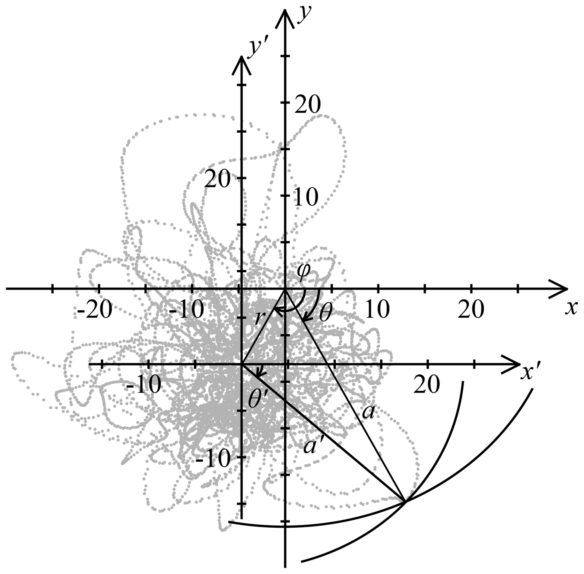
Figure 1 Schematics of relationships among variables used in this paper on the complex plane. x+iy is the total complex-valued amplitude, and $x^{\prime }+i{y}^{\prime }$ is that with zero mean. Grey dots show samples taken from nonharmonic vertical-mode-one semidiurnal internal tide at the PIL200 location (described in the Methods section). For illustration purposes, r=9 m (≈1.5 times the standard deviation of harmonic semidiurnal internal tide) and φ=120° are chosen arbitrarily.

Following previous studies cited in the Introduction, nonharmonic internal tides are defined by subtracting harmonic internal tides estimated by harmonic analysis (i.e. least-squares fitting of sinusoids at the tidal frequencies). So, we consider the statistics of

$$\begin{array}{}\text{(2)}& \begin{array}{rl}{X}^{\prime }+i{Y}^{\prime }& =(X+iY)-\left(\mathrm{E}\right(X)+i\mathrm{E}(Y\left)\right)\\ & =\sum _{j=\mathrm{1}}^N\left\{X_j+i{Y}_j-\left(\mathrm{E}\left(X_j\right)+i\mathrm{E}\left(Y_j\right)\right)\right\}\end{array}\end{array}$$

in this study. Hereafter, E(⋅) denotes the expected value of the argument. We write the above expression in polar form as

$$\begin{array}{}\text{(3)}& \begin{array}{rl}{A}^{\prime }{e}^{-i{\mathrm{\Theta }}^{\prime }}& =A{\mathrm{e}}^{-i\mathrm{\Theta }}-r{e}^{-i\mathit{\phi }}\\ & =\sum _{j=\mathrm{1}}^N\left\{A_j{e}^{-i{\mathrm{\Theta }}_j}-r_j{e}^{-i{\mathit{\phi }}_j}\right\},\end{array}\end{array}$$

where $\mathrm{E}\left(X\right)+i\mathrm{E}\left(Y\right)=r{e}^{-i\mathit{\phi }}$. Note that r is the distance to the expected value of the complex vector X+iY on the complex plane. Because of this, $\mathrm{E}\left(A{{}^{\prime }}^{\mathrm{2}}\right)$ is not Var(A), and r and φ are not E(A) and E(Θ), respectively. Hereafter, Var(⋅) denotes the variance of the argument. Relationships among the variables are illustrated in Fig. 1.

A particular variable of interest in this study is $A{{}^{\prime }}^{\mathrm{2}}$, which corresponds to the squared envelope amplitude of a nonharmonic internal tide. It may not be obvious in the polar form, but provided that the individual sinusoidal components are independent, the use of Cartesian components shows that the following relationship generally holds for non-identically distributed components, without assuming the independence of $A_j^{\prime }$ and ${\mathrm{\Theta }}_j^{\prime }$:

$$\begin{array}{}\text{(4)}& \begin{array}{rl}E\left(A{{}^{\prime }}^{\mathrm{2}}\right)& =E\left(X{{}^{\prime }}^{\mathrm{2}}+Y{{}^{\prime }}^{\mathrm{2}}\right)\\ & =\sum _{j=\mathrm{1}}^{N}E\left(X{{}_j^{\prime }}^{\mathrm{2}}\right)+\sum _{j=\mathrm{1}}^{N}E\left(Y{{}_j^{\prime }}^{\mathrm{2}}\right)\\ & =\sum _{j=\mathrm{1}}^{N}E\left(A{{}_j^{\prime }}^{\mathrm{2}}\right).\end{array}\end{array}$$

In this study, we refer to the second moment of A^′ as the “total variance”, and write ${\mathit{\sigma }}_{A^{\prime }}^{\mathrm{2}}=\mathrm{E}\left({A^{\prime }}^{\mathrm{2}}\right)$ because it is the sum of Var(X) and Var(Y), although it is not Var(A).

2.1 Probability distribution functions in the many source limit

Since we consider a sum of random variables, the central limit theorem in statistics suggests the existence of a universal PDF in the limit of large N, which is applicable regardless of the PDFs of the individual wave components. Hereafter, the limit of large N is referred to as the “many source limit“ because individual components in Eqs. (1)–(4) require wave sources. We derive a statistical model in the many source limit in this section because only the many source limit is considered in the majority of this paper. The model is a simplified version of the general model applicable to arbitrary N, which is required to investigate the rate of convergence to the many source limit with increasing N. Since this general model requires mathematics rather specific to statistics, the derivation is presented in Appendix A. The relationships in this section are applicable to general PDFs of the individual wave components, and specific PDFs are introduced in the following section.

Before deriving the statistical model in the many source limit, it is necessary to note one detailed point in statistics, which is required to derive PDFs in the many source limit. If we write the joint PDF in Cartesian coordinates as f_XY and in polar coordinates as f_AΘ, the two are related as

$$\begin{array}{}\text{(5)}& f_{XY}(x,y)\mathrm{d}x\mathrm{d}y=f_{A\mathrm{\Theta }}(a,\mathit{\theta })\mathrm{d}a\mathrm{d}\mathit{\theta }\end{array}$$

in the convention in statistics (Hoyt, 1947). Note that the Jacobian of the coordinate transformation (i.e. a) is included in f_AΘ so that $f_{XY}=a^{-\mathrm{1}}{f}_{A\mathrm{\Theta }}$ (Hoyt, 1947). This is necessary to make the integral of f_AΘ over the whole domain unity and to retain the properties of PDFs (e.g. marginal and conditional probability); however, it is unfortunately a potential source of confusion because they do not follow the standard rule of coordinate transformation.

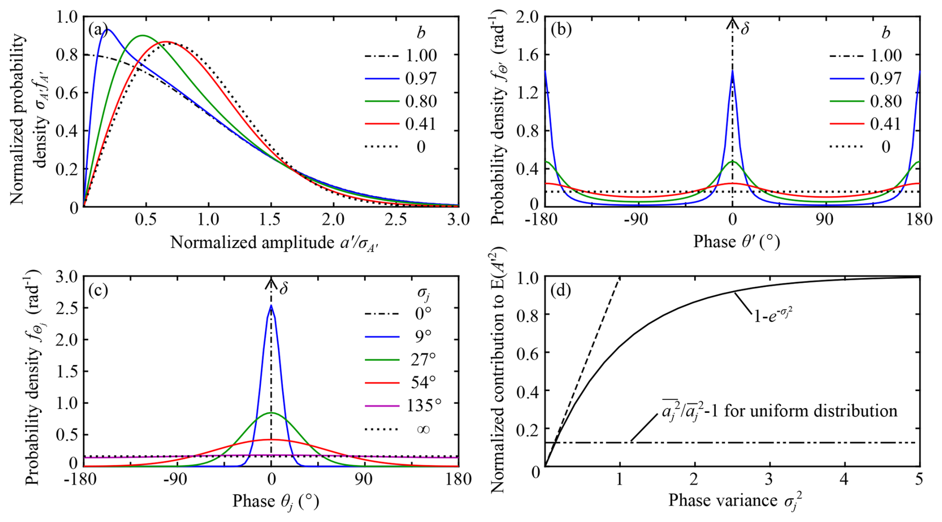
Figure 2 Analytic probability density functions (PDFs) used in this paper and their properties. (a) Generalized Rayleigh distribution in Eq. (9a), (b) phase distribution of joint Gaussian distribution in Eq. (9b) plotted with ${\mathit{\phi }}_{\mathrm{P}}^{\prime }=\mathrm{0}$, (c) wrapped normal phase distribution in Eq. (12) plotted with φ_j=0, and (d) normalized contributions to $\mathrm{E}\left({A^{\prime }}^{\mathrm{2}}\right)$ (the dashed double-dotted line and solid line show the first and second terms of Eq. 14b, respectively). In (a), amplitude and PDFs are normalized by envelope-amplitude standard deviation ${\mathit{\sigma }}_{A{}^{\prime }}$. In (b) and (c), lines with an upward arrow indicate the Dirac delta function. For sinusoidal components with equal amplitude and phase lag, distributions in (a) and (b) are limiting distributions for large N under the phase distribution in (c) with the same line style.

We now proceed to deriving the statistical model in the many source limit. When N is sufficiently large, and Var(X_j)≪Var(X) and Var(Y_j)≪Var(Y) for all j indices in Eq. (4) (i.e. none of the components dominate the variance), the central limit theorem states that X^′ and Y^′ are asymptotically normally distributed (Beckmann, 1964). Then, the joint probability distribution of X^′ and Y^′ approaches the joint Gaussian distribution. To simplify the mathematical expression, it is convenient to rotate the (x^′, y^′) axes on the complex plane to the so-called principal axes ($x_{\mathrm{P}}^{\prime }$, $y_{\mathrm{P}}^{\prime }$) so that $X_{\mathrm{P}}^{\prime }$ and $Y_{\mathrm{P}}^{\prime }$ are uncorrelated. The direction of the principal axes is found from the covariance matrix

$$\begin{array}{}\text{(6)}& \mathbf{C}=\left[\begin{array}{cc}{\mathit{\sigma }}_X^{\mathrm{2}}& {\mathit{\rho }}_{XY}{\mathit{\sigma }}_X{\mathit{\sigma }}_Y\\ {\mathit{\rho }}_{XY}{\mathit{\sigma }}_X{\mathit{\sigma }}_Y& {\mathit{\sigma }}_Y^{\mathrm{2}}\end{array}\right],\end{array}$$

where σ_X and σ_Y are the standard deviation of X^′ and Y^′, respectively, and ρ_XY is the correlation coefficient of X^′ and Y^′. The eigenvalues of C provide the variance in the major and minor principal directions, ${\mathit{\sigma }}_{X_{\mathrm{P}}}^{\mathrm{2}}$ and ${\mathit{\sigma }}_{Y_{\mathrm{P}}}^{\mathrm{2}}(\le {\mathit{\sigma }}_{X_{\mathrm{P}}}^{\mathrm{2}})$, and the eigenvector provides the direction of the major principal axis, φ_P. Using the principal axes, the joint PDF $f_{X{}_{\mathrm{P}}^{\prime }Y{}_{\mathrm{P}}^{\prime }}$ approaches the joint Gaussian distribution:

$$\begin{array}{}\text{(7)}& f_{X{}_{\mathrm{P}}^{\prime }Y{}_{\mathrm{P}}^{\prime }}\left(x_{\mathrm{P}}^{\prime },y_{\mathrm{P}}^{\prime }\right)\sim {\displaystyle \frac{\mathrm{1}}{\mathrm{2}\mathit{\pi }{\mathit{\sigma }}_{X_{\mathrm{P}}}{\mathit{\sigma }}_{Y_{\mathrm{P}}}}}\exp \left(-{\displaystyle \frac{\mathrm{1}}{\mathrm{2}}}\left({\displaystyle \frac{x{{}_{\mathrm{P}}^{\prime }}^{\mathrm{2}}}{{\mathit{\sigma }}_{X_{\mathrm{P}}}^{\mathrm{2}}}}+{\displaystyle \frac{y{{}_{\mathrm{P}}^{\prime }}^{\mathrm{2}}}{{\mathit{\sigma }}_{Y_{\mathrm{P}}}^{\mathrm{2}}}}\right)\right).\end{array}$$

This can be written in polar coordinates as

$$\begin{array}{}\text{(8)}& \begin{array}{rl}& f_{A^{\prime }{\mathrm{\Theta }}^{\prime }}(a,\mathit{\theta })\sim {\displaystyle \frac{a}{\mathrm{2}\mathit{\pi }{\mathit{\sigma }}_{X_{\mathrm{P}}}{\mathit{\sigma }}_{Y_{\mathrm{P}}}}}\\ & \times \exp \left(-{\displaystyle \frac{a^{\mathrm{2}}}{\mathrm{4}}}\left({\displaystyle \frac{\mathrm{1}+\cos \mathrm{2}\left(\mathit{\theta }-{\mathit{\phi }}_{\mathrm{P}}\right)}{{\mathit{\sigma }}_{X_{\mathrm{P}}}^{\mathrm{2}}}}\right.\right.\left.\left.+{\displaystyle \frac{\mathrm{1}-\cos \mathrm{2}\left(\mathit{\theta }-{\mathit{\phi }}_{\mathrm{P}}\right)}{{\mathit{\sigma }}_{Y_{\mathrm{P}}}^{\mathrm{2}}}}\right)\right),\end{array}\end{array}$$

where $(x_{\mathrm{P}}^{\prime },y_{\mathrm{P}}^{\prime })=a\left(\cos \right(\mathit{\theta }-{\mathit{\phi }}_{\mathrm{P}}),\sin (\mathit{\theta }-{\mathit{\phi }}_{\mathrm{P}}\left)\right)$. (The prime is omitted from a and θ for brevity.) Note that a is multiplied to impose Eq. (5). The corresponding amplitude and phase distributions can be obtained by integrating $f_{A^{\prime }\mathrm{\Theta }{{}^{\prime }}_{\mathrm{P}}}$ over θ and a, respectively (i.e. marginal distributions). The integrations yield

$$\begin{array}{}\text{(9a)}& {\displaystyle }\begin{array}{rl}{f}_{A^{\prime }}\left(a\right)\sim & {\displaystyle \frac{\mathrm{2}a}{{\mathit{\sigma }}_{A^{\prime }}^{\mathrm{2}}\sqrt{\mathrm{1}-b^{\mathrm{2}}}}}\exp \left(-{\displaystyle \frac{a^{\mathrm{2}}}{\left(\mathrm{1}-b^{\mathrm{2}}\right){\mathit{\sigma }}_{A^{\prime }}^{\mathrm{2}}}}\right)\\ & \times I_{\mathrm{0}}\left({\displaystyle \frac{b{a}^{\mathrm{2}}}{\left(\mathrm{1}-b^{\mathrm{2}}\right){\mathit{\sigma }}_{A^{\prime }}^{\mathrm{2}}}}\right),\end{array}\text{(9b)}& {\displaystyle }\begin{array}{rl}& f_{{\mathrm{\Theta }}^{\prime }}\left(\mathit{\theta }\right)\sim {\displaystyle \frac{\mathrm{1}}{\mathrm{2}\mathit{\pi }}}{\displaystyle \frac{\sqrt{\mathrm{1}-b^{\mathrm{2}}}}{\mathrm{1}-b\cos \mathrm{2}\left(\mathit{\theta }-{\mathit{\phi }}_{\mathrm{P}}\right)}},\end{array}\text{(9c)}& {\displaystyle }\begin{array}{rl}& {\mathit{\sigma }}_{A^{\prime }}^{\mathrm{2}}={\mathit{\sigma }}_{X_{\mathrm{P}}}^{\mathrm{2}}+{\mathit{\sigma }}_{Y_{\mathrm{P}}}^{\mathrm{2}},\end{array}\text{(9d)}& {\displaystyle }\begin{array}{rl}& b={\mathit{\sigma }}_{A^{\prime }}^{-\mathrm{2}}\left({\mathit{\sigma }}_{X_{\mathrm{P}}}^{\mathrm{2}}-{\mathit{\sigma }}_{Y_{\mathrm{P}}}^{\mathrm{2}}\right).\end{array}\end{array}$$

Here, I₀ is the modified Bessel function of the first kind of the order 0, and the integral over θ is evaluated using

$$\begin{array}{}\text{(10)}& \underset{-\mathit{\pi }}{\overset{\mathit{\pi }}{\int }}{e}^{a\cos \mathit{\theta }}\mathrm{d}\mathit{\theta }=\mathrm{2}\mathit{\pi }{I}_{\mathrm{0}}\left(a\right),\end{array}$$

which comes from the so-called Jacobi–Anger expansion (Abramowitz and Stegun, 1972, Eq. 9.6.34 or DLMF, 2025, Eq. 10.35.2). As shown by Hoyt (1947), the radial distribution function is a generalization of the Rayleigh distribution (see also Nakagami, 1960; Beckmann, 1964). The distribution becomes the standard Rayleigh distribution when b=0 and approaches a one-sided Gaussian distribution when b→1 (Fig. 2a). The phase distribution is bimodal and becomes uniform when b=0 and two sharp peaks when b→1 (Fig. 2b). Note that ${\mathit{\sigma }}_{A^{\prime }}^{\mathrm{2}}=\mathrm{Var}\left(X\right)+\mathrm{Var}\left(Y\right)=\mathrm{E}\left({A^{\prime }}^{\mathrm{2}}\right)$ from the property of eigenvalues and Eq. (4) or Eqs. (A13a)–(A13b).

2.2 Specific probability distribution functions

To apply the above general relationships to nonharmonic internal tides, we assume specific amplitude and phase distributions. First, we assume that the amplitude and phase variability of each sinusoidal component are independent:

$$\begin{array}{}\text{(11)}& f_{A_j{\mathrm{\Theta }}_j}\left(a_j,{\mathit{\theta }}_j\right)=f_{A_j}\left(a_j\right)f_{{\mathrm{\Theta }}_j}\left({\mathit{\theta }}_j\right).\end{array}$$

Second, we assume that $f_{{\mathrm{\Theta }}_j}$ is given by the wrapped normal (or Gaussian) distribution (Mardia, 1972, p. 55)

$$\begin{array}{}\text{(12)}& f_{{\mathrm{\Theta }}_j}\left({\mathit{\theta }}_j\right)={\displaystyle \frac{\mathrm{1}}{\sqrt{\mathrm{2}\mathit{\pi }}{\mathit{\sigma }}_j}}\sum _{k=-\mathrm{\infty }}^{\mathrm{\infty }}\exp \left(-{\displaystyle \frac{{\left({\mathit{\theta }}_j-{\mathit{\phi }}_j+\mathrm{2}\mathit{\pi }k\right)}^{\mathrm{2}}}{\mathrm{2}{\mathit{\sigma }}_j^{\mathrm{2}}}}\right),\end{array}$$

where σ_j is the standard deviation of the phase and is shorthand notation for $\mathit{\sigma }{}_{{\mathrm{\Theta }}_j^{\prime }}$. The wrapped normal distribution is a circular analogue of the Gaussian distribution and defined for any one period of 2π. It approaches the Gaussian distribution in the limit σ_j→0 but approaches the uniform distribution in the limit σ_j→∞ (Fig. 2c). Note that we consider non-identical phase distribution (i.e. φ_j and σ_j are not necessary the same for different j indices). Then, the mean and second moments under Eq. (12) are given by

$$\begin{array}{}\text{(13a)}& {\displaystyle }& {\displaystyle }E\left(X_j+i{Y}_j\right)=r_j{e}^{-i{\mathit{\phi }}_j},\text{(13b)}& {\displaystyle }& {\displaystyle }E\left(A{{}_j^{\prime }}^{\mathrm{2}}\right)=\stackrel{\mathrm{‾}}{a_j^{\mathrm{2}}}-r_j^{\mathrm{2}}={\stackrel{\mathrm{‾}}{a}}_j^{\mathrm{2}}{\mathit{\varsigma }}_j^{\mathrm{2}},\text{(13c)}& {\displaystyle }& {\displaystyle }E\left(X{{}_j^{\prime }}^{\mathrm{2}}\right)={\displaystyle \frac{\mathrm{1}}{\mathrm{2}}}{\stackrel{\mathrm{‾}}{a}}_j^{\mathrm{2}}{\mathit{\varsigma }}_j^{\mathrm{2}}+{\displaystyle \frac{\mathrm{1}}{\mathrm{2}}}\left(\stackrel{\mathrm{‾}}{a_j^{\mathrm{2}}}{e}^{-\mathrm{2}{\mathit{\sigma }}_j^{\mathrm{2}}}-r_j^{\mathrm{2}}\right)\cos \mathrm{2}{\mathit{\phi }}_j,\text{(13d)}& {\displaystyle }& {\displaystyle }E\left(Y{{}_j^{\prime }}^{\mathrm{2}}\right)={\displaystyle \frac{\mathrm{1}}{\mathrm{2}}}{\stackrel{\mathrm{‾}}{a}}_j^{\mathrm{2}}{\mathit{\varsigma }}_j^{\mathrm{2}}-{\displaystyle \frac{\mathrm{1}}{\mathrm{2}}}\left(\stackrel{\mathrm{‾}}{a_j^{\mathrm{2}}}{e}^{-\mathrm{2}{\mathit{\sigma }}_j^{\mathrm{2}}}-r_j^{\mathrm{2}}\right)\cos \mathrm{2}{\mathit{\phi }}_j,\text{(13e)}& {\displaystyle }& {\displaystyle }E\left(X{}_j^{\prime }Y{}_j^{\prime }\right)=-{\displaystyle \frac{\mathrm{1}}{\mathrm{2}}}\left(\stackrel{\mathrm{‾}}{a_j^{\mathrm{2}}}{e}^{-\mathrm{2}{\mathit{\sigma }}_j^{\mathrm{2}}}-r_j^{\mathrm{2}}\right)\sin \mathrm{2}{\mathit{\phi }}_j,\end{array}$$

where

$$\begin{array}{}\text{(14a)}& {\displaystyle }& {\displaystyle }{r}_j={\stackrel{\mathrm{‾}}{a}}_j{e}^{-{\mathit{\sigma }}_j^{\mathrm{2}}/\mathrm{2}},\text{(14b)}& {\displaystyle }& {\displaystyle }{\mathit{\varsigma }}_j^{\mathrm{2}}=\left({\displaystyle \frac{\stackrel{\mathrm{‾}}{a_j^{\mathrm{2}}}}{{\stackrel{\mathrm{‾}}{a}}_j^{\mathrm{2}}}}-\mathrm{1}\right)+\left(\mathrm{1}-e^{-{\mathit{\sigma }}_j^{\mathrm{2}}}\right),\end{array}$$

and ${\stackrel{\mathrm{‾}}{a}}_j=\mathrm{E}\left(A_j\right)$ and $\stackrel{\mathrm{‾}}{a_j^{\mathrm{2}}}=E\left(A_j^{\mathrm{2}}\right)$. As seen in these relationships, and as shown before by Colosi and Munk (2006), the phase spread σ_j provides a convenient way to separate the variance of each sinusoid ($\stackrel{\mathrm{‾}}{a_j^{\mathrm{2}}}$) into the deterministic (mean) component ($r_j^{\mathrm{2}}$) and the random (deviation) component (${\stackrel{\mathrm{‾}}{a}}_j^{\mathrm{2}}{\mathit{\varsigma }}_j^{\mathrm{2}}$). It is also convenient that the random component is separated into the contributions from random amplitude (the first term in ${\mathit{\varsigma }}_j^{\mathrm{2}}$) and random phase (the second term).

We also need the amplitude distribution $f_{A_j}$ to solve the problem, and we consider two contrasting amplitude PDFs. The first amplitude PDF is the constant (deterministic) distribution:

$$\begin{array}{}\text{(15)}& f_{A_j}\left(a_j\right)=\mathit{\delta }\left(a_j-{\mathit{\sigma }}_{A_j}\right),\end{array}$$

where ${\mathit{\sigma }}_{A_j}$ is the constant amplitude (and $\mathrm{E}(A_j^{\mathrm{2}}{)}^{\mathrm{1}/\mathrm{2}}$), and δ(⋅) denotes the Dirac delta function. In this case, ${\stackrel{\mathrm{‾}}{a}}_j={\mathit{\sigma }}_{A_j}$ and $\stackrel{\mathrm{‾}}{a_j^{\mathrm{2}}}={\mathit{\sigma }}_{A_j}^{\mathrm{2}}$. The second amplitude PDF is the uniform distribution:

$$\begin{array}{}\text{(16)}& f_{A_j}\left(a_j\right)=\left\{\begin{array}{ll}\frac{a_j}{{\mathit{\sigma }}_{A_j}^{\mathrm{2}}}& \mathrm{for}{a}_j\le \sqrt{\mathrm{2}}{\mathit{\sigma }}_{A_j}\\ \mathrm{0}& \mathrm{for}{a}_j>\sqrt{\mathrm{2}}{\mathit{\sigma }}_{A_j}\end{array}\right..\end{array}$$

This distribution is referred to as “uniform” because it corresponds to uniform probability in the radial direction between 0 and $\sqrt{\mathrm{2}}{\mathit{\sigma }}_{A_j}$ on the x_j–y_j plane. (Note that the factor a_j comes from the requirement in Eq. 5.) The distribution is normalized to have $\stackrel{\mathrm{‾}}{a_j^{\mathrm{2}}}={\mathit{\sigma }}_{A_j}^{\mathrm{2}}$, as in the constant-amplitude PDF. The mean amplitude is given by ${\stackrel{\mathrm{‾}}{a}}_j=\mathrm{2}\sqrt{\mathrm{2}}{\mathit{\sigma }}_{A_j}/\mathrm{3}$.

The specific phase and amplitude distributions allow the evaluation of the second moments in Eqs. (13b)–(13e). Then, because of Eq. (4), ${\mathit{\sigma }}_{A^{\prime }}$ in the limiting distribution (Eqs. 9a and 9b) is given by the square root of the sum of $\mathrm{E}\left(A{{}_j^{\prime }}^{\mathrm{2}}\right)$. The b parameter in the limiting distribution can be calculated from the eigenvalues of the covariance matrix (Eq. 6), whose components are given by the sum of $\mathrm{E}\left(X{{}_j^{\prime }}^{\mathrm{2}}\right)$, $\mathrm{E}\left(Y{{}_j^{\prime }}^{\mathrm{2}}\right)$, and $\mathrm{E}\left(X{}_j^{\prime }Y{}_j^{\prime }\right)$.

It is worth noting here that the relationships under the wrapped normal distribution suggest relatively small effects of amplitude distribution on the total amplitude A^′ for two reasons. The first reason is that the contribution of random amplitude to the total variance is relatively small. The first term in Eq. (14b) is 0 (constant) and $\mathrm{1}/\mathrm{8}$ (uniform) for these very different amplitude distributions. In comparison, the second term can be as large as 1 (Fig. 2d) without requiring a large phase spread, as pointed out by Zaron and Egbert (2014). For example, the e-folding variance (where the dashed line reaches 1 in Fig. 2d) is about 1, or 16 % of the full phase 2π in terms of standard deviation. The second reason is that the general version of the statistical model in Appendix A suggests that random amplitude (or smooth $f_{A_j}$) tends to smooth the Fourier transform of the PDF (i.e. characteristic function) ϕ_j compared to the constant-amplitude case (Eq. A14). This means that random amplitude tends to make the total-amplitude PDF $f_{A^{\prime }}$ smoother and to make the convergence to the limiting distributions (Eqs. 9a and 9b) faster. For these reasons, we consider rather contrasting amplitude distributions $f_{A_j}$ in this paper.

It is also worth noting that the wrapped normal distribution is similar to the von Mises distribution used, for example, by Barakat (1988), and both distributions yield similar results within the scope of this paper. However, the two distributions are different in that the phase spread parameter in the von Mises distribution is not the standard deviation and lacks clear meaning when the distribution deviates significantly from the Gaussian distribution, whereas the phase spread parameter of the wrapped normal distribution is the standard deviation and could be estimated by various means. The wrapped normal distribution is chosen in this paper so that a stochastic model can be used to estimate the phase spread parameter in Part 2 of this study (Shimizu, 2025).

3 Methods

3.1 Calculation of theoretical probability density function

We investigated the convergence rate of the PDFs to the limiting distributions (Eqs. 9a and 9b) by calculating PDFs and covariance matrices using the general version of the statistical model in Appendix A under the specific phase and amplitude distributions in Sect. 2.2 and varying N. The details of the computation are provided in Appendix A.

3.2 PIL200 observations

We investigated the applicability of the proposed statistical model to nonharmonic internal tides by comparing the statistical model with measurements at the PIL200 location on the Australian North West Shelf (115.915° E, 19.435° S; water depth ≈200 m). A mooring consisting of CTDs, thermistors, and an acoustic Doppler current profiler (ADCP) was deployed from 20 February 2012 to 18 August 2014 as part of the Australian Integrated Marine Observing System (IMOS). The measurements consisted of five half-yearly deployments. Although the number and heights of instruments as well as instrument settings varied over the whole measurement period, temperature and salinity were overall measured at approximately 10 and 20–30 m intervals, respectively, over the whole water column except in the upper 20–30 m. Typical sampling intervals of the CTDs and thermistors were either 60 or 120 s. Current velocity was measured at 10 m vertical intervals, and the sampling intervals varied between 300 and 1200 s among the five deployments. Pressure was measured by the ADCP located at 8–9 m above the seabed.

The PIL200 data were processed as follows. We retained only data flagged as “Good_data” and “Probably_good_data” and removed suspicious salinity records. Then, we interpolated salinity to the thermistor depths, removed high-frequency variability by low-pass-filtering temperature and salinity with a cut-off period of ≈1 h, subsampled them at 15 min intervals, and calculated isopycnal elevation. When vertical salinity interpolation was difficult because of bad or missing data at multiple levels, we did not attempt to calculate isopycnal elevation. We used isopycnal densities from 1021.00 to 1026.25 kg m⁻³ at 0.25 kg m⁻³ intervals, which resulted in roughly one isopycnal every 10 m. Surface elevation was calculated from the pressure measurements and then low-pass-filtered and subsampled in the same way. Then, we calculated surface and isopycnal displacements by subtracting the corresponding background elevation, calculated by low-pass-filtering the isopycnal elevation with a cut-off period of ≈62 h to remove tidal and inertial variability. Current velocity was processed similarly by removing high-frequency variability, by subsampling, and then by subtracting the background (low-frequency) currents.

3.3 Vertical-mode amplitude estimation

We considered vertical-mode-one (VM1) to mode-four (VM4) internal tides, whose amplitudes and energetics were estimated as follows.

We calculated the first five modes (${\widehat{\mathit{\varphi }}}_n$ for $n=\mathrm{0},\mathrm{1},\mathrm{2},\mathrm{3},\mathrm{4}$) and the associated celerities (c_n) as a function of time (at 15 min intervals) using the low-pass-filtered (background) isopycnal elevation and the formulation of vertical modes in Shimizu (2017, 2019). (In this study, the term “celerity” is deliberately used for the propagation speed of non-rotating, long, linear gravity waves with one of the vertical-mode structures, which differs from the phase speed of internal tides.) Hereafter, the subscript n denotes mode index, which is 0 for the barotropic mode, 1 for VM1 (the first baroclinic mode), etc. The most common normalization of vertical modes is to set the maximum value to 1; however, for numerically computed vertical modes, this normalization can introduce discontinuous changes as the stratification varies over time. In this paper, the vertical modes were normalized by setting the arbitrary norm for the barotropic mode (${\widehat{h}}_{\mathrm{0}}$) to the water depth (201 m) and the norms for VM1 (${\widehat{h}}_{\mathrm{1}}$), VM2 (${\widehat{h}}_{\mathrm{2}}$), VM3 (${\widehat{h}}_{\mathrm{3}}$), and VM4 (${\widehat{h}}_{\mathrm{4}}$) to 1$/$5, 1$/$17, 1$/$38, and 1$/$63 of the water depth, respectively. The celerities of baroclinic modes showed clear seasonal variation, but the above normalization of the vertical modes kept the extreme (minimum or maximum) value of ${\widehat{\mathit{\varphi }}}_n$ at about 1 (black line in Fig. 3a and b). (However, note that the depths of the extreme varied seasonally.)

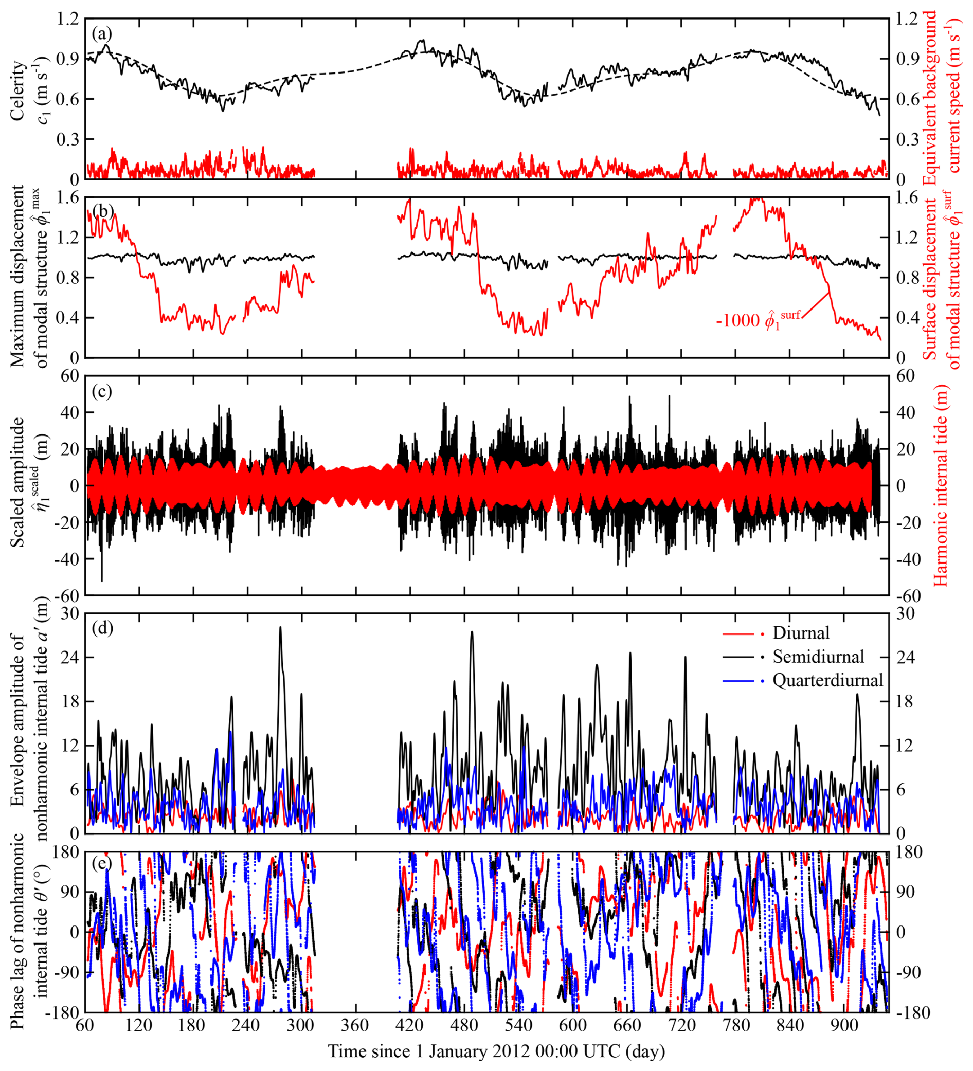
Figure 3 Time series of variables related to vertical-mode-one (VM1) internal tides from PIL200 observations. (a) Celerity and low-pass-filtered (subtidal) background VM1 current speed, (b) maximum and surface values of VM1 structure function, (c) scaled isopycnal displacement amplitude and its harmonic component, and (d, e) envelope amplitudes and Greenwich phase lags of diurnal, semidiurnal, and quarter-diurnal components of nonharmonic internal tides. In (a), the dashed line shows least-squares fit of annual and semi-annual cycles to celerity.

Using the vertical modes, we estimated vertical-mode amplitudes of isopycnal displacement (${\widehat{\mathit{\eta }}}_n$) and the horizontal velocity vector (${\widehat{\overrightarrow{v}}}_n$) based on the Gauss–Markov estimation (Wunsch, 1997). (The units of ${\widehat{\mathit{\eta }}}_n$ and ${\widehat{\overrightarrow{v}}}_n$ are metres and m s⁻¹, respectively.) This method required estimates of the error covariance, as well as the covariance of vertical-mode amplitudes. Following Wunsch (1997), we assumed diagonal covariance matrices. From the high-frequency end of the power spectra of the unfiltered time series, the standard deviations of surface displacement, isopycnal displacement, and horizontal velocity errors were estimated to be ≈0.03 m, ≈3 m, and ≈0.04 m s⁻¹, respectively. The prior estimates of vertically integrated available potential or kinetic energies contained in the first five modes were set to 1000, 1000, 500, 250, and 125 J m⁻² (the energy ratio was taken from Wunsch, 1997). Since the extreme values of ${\widehat{\mathit{\varphi }}}_n$ are about 1, ${\widehat{\mathit{\eta }}}_n$ corresponds to the maximum or minimum isopycnal displacement within the water column.

Since the measurements were made on the continental shelf, the seasonal variability of stratification affected vertical modes and related variables substantially (e.g. the black line in Fig. 3a), including ${\widehat{\mathit{\eta }}}_n\left(t\right)$ (not shown). Although harmonic analysis with multi-year-long records can determine seasonally variable harmonic internal tides, non-random seasonal variation of nonharmonic internal tides, which is not considered in the statistical model, would make comparisons with the proposed statistical model more difficult. Therefore, to suppress the seasonal variability, we scaled the VM1 isopycnal displacement amplitude as

$$\begin{array}{}\text{(17)}& {\widehat{\mathit{\eta }}}_n^{\mathrm{scaled}}\left(t\right)={\displaystyle \frac{c_n\left(t\right)}{c_n^{\mathrm{ref}}}}{\widehat{\mathit{\eta }}}_n\left(t\right),\end{array}$$

where $c_n^{\mathrm{ref}}$ (0.79 and 0.38 m s⁻¹ for VM1 and VM2, respectively) is the root mean square of c_n(t).

The vertically integrated available potential energy, kinetic energy, and energy flux are given by (Shimizu, 2011)

$$\begin{array}{}\text{(18a)}& {\displaystyle }& {\displaystyle }{P}_n\left(t\right)={\displaystyle \frac{\mathrm{1}}{\mathrm{2}}}\widehat{\mathit{\rho }}{\displaystyle \frac{c_n(t{)}^{\mathrm{2}}}{{\widehat{h}}_n}}{\widehat{\mathit{\eta }}}_n(t{)}^{\mathrm{2}},\text{(18b)}& {\displaystyle }& {\displaystyle }{K}_n\left(t\right)={\displaystyle \frac{\mathrm{1}}{\mathrm{2}}}\widehat{\mathit{\rho }}{\widehat{h}}_n\left|{\widehat{\overrightarrow{v}}}_n\right(t){|}^{\mathrm{2}},\text{(18c)}& {\displaystyle }& {\displaystyle }{\overrightarrow{J}}_n\left(t\right)=\widehat{\mathit{\rho }}{c}_n\left(t{)}^{\mathrm{2}}{\widehat{\mathit{\eta }}}_n\right(t\left){\widehat{\overrightarrow{v}}}_n\right(t),\end{array}$$

where $\widehat{\mathit{\rho }}$ is the constant reference density used in vertical-mode calculation (1025 kg m⁻³). Since P_n is given by Eq. (18a), the scaled amplitude in Eq. (17) is proportional to the square root of the available potential energy, rather than the vertical displacement of isopycnals.

Please note that the scaling in Eq. (17) suppresses seasonal variability in the following analyses but does not remove the seasonality in any way. It merely uses the fact that available potential energy showed less seasonality than isopycnal displacements. Since the product ${\widehat{\mathit{\varphi }}}_n{\widehat{\mathit{\eta }}}_n$ is a physically meaningful quantity that has to remain the same regardless of the scaling of vertical modes, the scaling in Eq. (17) makes the scaled vertical mode (i.e. ${\widehat{\mathit{\varphi }}}_n^{\mathrm{scaled}}=c_n^{-\mathrm{1}}{c}_n^{\mathrm{ref}}{\widehat{\mathit{\varphi }}}_n$) more seasonally variable. Also, note that the surface expression of internal tides showed seasonal variability with or without the scaling (Fig. 3b), which might be relevant for satellite altimetry but is not the focus of this paper.

The scaled isopycnal displacement amplitudes ${\widehat{\mathit{\eta }}}_n^{\mathrm{scaled}}\left(t\right)$ are the main variables analysed in this paper. The horizontal velocity amplitudes ${\widehat{\overrightarrow{v}}}_n\left(t\right)$ are used only for obtaining some diagnostics and for some discussion.

3.4 Harmonic analysis

The T_TIDE package (Pawlowicz et al., 2002) was used for the traditional harmonic analysis (Foreman, 1977) to estimate harmonic internal tides. The whole record of ${\widehat{\mathit{\eta }}}_n^{\mathrm{scaled}}\left(t\right)$ was used to estimate one set of harmonic constants. For consistency, we opted to use the common constituents used in the previous studies of nonharmonic internal tides (i.e. M₂, S₂, N₂, K₂, K₁, O₁, P₁, Q₁), although the multi-year record length allowed the determination of more constituents. There were two exceptions to this. The first exception was that we included the seasonal cycle of M₂ and S₂ constituents (which are represented by the H₁, H₂, R₂, and T₂ constituents in the T_TIDE package) because a small seasonal cycle remained after the scaling in Eq. (17). The second exception was that we included M₄, MS₄, and S₄ quarter-diurnal tides (or shallow-water tides, which are overtides and compound tides of semidiurnal constituents) because the PIL200 location was on the continental shelf and the spectral analysis, described below, showed clear quarter-diurnal peaks.

3.5 Nonharmonic internal tides

Nonharmonic internal tides were determined by subtracting the harmonic internal tides from ${\widehat{\mathit{\eta }}}_n^{\mathrm{scaled}}\left(t\right)$. We analysed the diurnal, semidiurnal, and quarter-diurnal components. They were calculated by bandpass-filtering the time series in the 21–28, 11–15, and 5.8–6.7 h bands, respectively. These bands were determined by the widths of the corresponding spectral peaks of nonharmonic internal tides. The envelope amplitude a^′(t) of each component was estimated by first low-pass-filtering the squared time series and then multiplying the results by 2, which comes from the mean square of the sinusoidal “carrier” wave. Then, the phase lag θ^′(t) was found by local least-squares fitting of a sinusoid to the time series normalized by the envelope amplitude over one period. (This method appeared to be more robust than the Hilbert transform.) The phase lag of each component was calculated as a Greenwich phase lag with respect to the dominant constituent (K₁, M₂, and M₄ for the diurnal, semidiurnal, and quarter-diurnal components, respectively). The record length of the PIL200 observations (>2 years) was considered to be sufficiently long to analyse the statistics of nonharmonic internal tides on a continental shelf, although the uncertainties are relatively large as shown later.

3.6 Spectral analysis and estimation of cusp parameters

The power spectral densities (PSDs) of the total and nonharmonic internal tides were estimated by calculating the periodogram of half-overlapping ≈85 d records (2¹³ data points) of the corresponding time series with the Hamming window, averaging them, and then converting the results to PSD. Throughout this study, PSD is defined as one-sided, defined for $\mathrm{0}\le \mathit{\omega }<\mathrm{\infty }$, to be consistent with harmonic analysis.

For the goodness-of-fit test described below, the equivalent degrees of freedom (e.g. von Storch and Zwiers, 1999, chap. 17.1) of the nonharmonic internal-tide time series were required. The most straightforward way to estimate them was to use e-folding decorrelation times from the shapes of so-called “cusps” in the estimated PSD, following Colosi and Munk (2006) and Zaron (2022). These studies fit one Lorentzian spectrum above a constant background level to a frequency band containing a cusp; however, two Lorentzian spectra were used in this paper because a cusp covered multiple major tidal constituents, and their frequency differences were not always negligible compared to the cusp width. This double Lorentzian spectral model is

$$\begin{array}{}\text{(19)}& \begin{array}{rl}& g\left(\mathit{\omega };{\mathit{\sigma }}_{A^{\prime }}^{\mathrm{2}},T_{\mathit{\eta }},\mathit{\beta },S_{\mathrm{0}}\right)={\displaystyle \frac{{\mathit{\sigma }}_{A^{\prime }}^{\mathrm{2}}}{\mathrm{2}\mathit{\pi }{T}_{\mathit{\eta }}}}\\ & \times \left({\displaystyle \frac{\mathit{\beta }}{{\left(\mathit{\omega }-{\mathit{\omega }}_{\mathrm{1}}\right)}^{\mathrm{2}}+T_{\mathit{\eta }}^{-\mathrm{2}}}}\right.\left.+{\displaystyle \frac{(\mathrm{1}-\mathit{\beta })}{{\left(\mathit{\omega }-{\mathit{\omega }}_{\mathrm{2}}\right)}^{\mathrm{2}}+T_{\mathit{\eta }}^{-\mathrm{2}}}}\right)+S_{\mathrm{0}},\end{array}\end{array}$$

where ${\mathit{\sigma }}_{A^{\prime }}^{\mathrm{2}}$ is the total variance of envelope amplitude in a cusp, T_η is the e-folding decorrelation time, ω₁ and ω₂ are the angular frequencies of two tidal constituents, β is the fraction of variance associated with the first constituent, and S₀ is the background spectral level. (There are additional terms for one-sided spectra, but they are negligible for ω₁T_η≫1 and ω₂T_η≫1.) For the diurnal, semidiurnal, and quarter-diurnal bands, the sets of (O₁, K₁), (M₂, S₂), and (M₄, MS₄) constituents were used, respectively.

For cusps with an approximately Lorentzian form, the parameters ${\mathit{\sigma }}_{A^{\prime }}^{\mathrm{2}}$, T_η, β, and S₀ were estimated by least-squares fitting as follows. The most straightforward least-squares fitting turned out to be unsatisfactory because the background level S₀ could become unrealistically low or negative. So, we used a variant of the weighted and tapered least squares (Wunsch, 2006, chap. 2.4.2), with a cost function similar to that used in data assimilation (Wunsch, 2006; Bennett, 2002):

$$\begin{array}{}\text{(20)}& \begin{array}{rl}{\displaystyle \frac{\mathrm{1}}{N_y}}& (\mathit{y}-g(\mathit{x};\mathit{p}\left){)}^T{\mathbf{R}}_{nn}^{-\mathrm{1}}\right(\mathit{y}-g(\mathit{x};\mathit{p}))\\ & +{\displaystyle \frac{\mathrm{1}}{N_p}}{\left(\mathit{p}-{\mathit{p}}_{\mathrm{init}}\right)}^T{\mathbf{R}}_{pp}^{-\mathrm{1}}\left(\mathit{p}-{\mathit{p}}_{\mathrm{init}}\right).\end{array}\end{array}$$

Here, the vector y contains the estimated PSD, the vector x contains ω where the PSDs are estimated, and the vector p contains the model parameters ${\mathit{\sigma }}_{A^{\prime }}^{\mathrm{2}}$, $T_{\mathit{\eta }}^{-\mathrm{1}}$, β, and S₀. The vector p_init is the initial guess of p, and R_nn and R_pp are the error covariance matrices of ($\mathit{y}-g(\mathit{x};\mathit{p})$) and (p−p_init), respectively. Diagonal R_nn and R_pp were assumed. The two terms were normalized by the number of respective vector elements N_y and N_p so that varying N_y for different frequency bands did not change the relative weight of the two terms. The initial guesses of T_η and S₀ were obtained by visual inspection of the estimated PSD. Visual guesses of $T_{\mathit{\eta }}^{-\mathrm{1}}$ were uncertain, and 1$/$14, 1$/$7, and 1$/$3.5 d⁻¹ were used as rough estimates for the diurnal, semidiurnal, and quarter-diurnal bands, respectively. The error of $T_{\mathit{\eta }}^{-\mathrm{1}}$ was assumed to be 50 %. The errors of the estimated PSD and S₀ were taken from half of the 95 % confidence intervals of the spectral estimate. The initial ${\mathit{\sigma }}_{A^{\prime }}^{\mathrm{2}}$ was taken from the variance of bandpass-filtered nonharmonic internal-tide time series. Since this estimate included the background level but ${\mathit{\sigma }}_{A^{\prime }}^{\mathrm{2}}$ does not, the initial guess of the background level was used for its error estimate. The initial β was taken from the variance ratio of harmonic internal tides in the two constituents, and the error of β was assumed to be 0.25. The minimum of Eq. (20) was searched for numerically.

3.7 Estimation of model parameters

To compare the statistical model with the PIL200 observations, we applied the statistical model in Sect. 2 to the diurnal, semidiurnal, and quarter-diurnal frequency bands rather than to each constituent. This is because it was impractical to separate nonharmonic internal tides into individual constituents. Although this means that the mean components, (r, φ), vary with time due to the existence of multiple constituents, it did not cause any difficulty because harmonic tides were subtracted before analysing nonharmonic internal tides.

For the comparisons, the parameters of the PDFs in the “many source” limit (Eqs. 9a and 9b) were estimated from each frequency component of nonharmonic internal tides as follows. From the envelope amplitude a^′(t) and phase θ^′(t), we first calculated the Cartesian counterparts, x^′(t) and y^′(t), and then estimated the covariance matrix C in Eq. (6). The parameters ${\mathit{\sigma }}_{A^{\prime }}$, b, and ${\mathit{\phi }}_{\mathrm{p}}^{\prime }$ were calculated from the eigenvalues and eigenvectors of C. This method appeared to be more robust than estimating the b parameter from the skewness of the envelope-amplitude distribution $f_{A^{\prime }}$.

Note that the variance of envelope amplitude ${\mathit{\sigma }}_{A^{\prime }}^{\mathrm{2}}$ is twice the variance of the original time series because the sinusoidal carrier wave was removed to calculate the envelope amplitude a^′(t). Note also that the background level in the PSD is included in ${\mathit{\sigma }}_{A^{\prime }}^{\mathrm{2}}$ estimated in this way but excluded in ${\mathit{\sigma }}_{A^{\prime }}^{\mathrm{2}}$ estimated by fitting the double Lorentzian model.

3.8 Goodness-of-fit test

The Pearson's χ² goodness-of-fit test was used to quantitatively compare the observed PDFs with the distributions in the many source limit because it is nonparametric and can be used with estimated parameters. To increase the reliability, the envelope amplitudes were binned with variable bin widths that correspond to equal probability under the standard Rayleigh distribution. The phases were binned with a constant bin width. The equivalent sample size (or degrees of freedom) was calculated by dividing the record length by twice the e-folding decorrelation time T_η (von Storch and Zwiers, 1999), estimated by the least-squares fitting of the double Lorentzian model to cusps in the PSD.

Note that the results of the goodness-of-fit test need to be interpreted with caution because the statistical model for a fixed frequency is compared to the observations in the diurnal, semidiurnal, and quarter-diurnal frequency bands.

4 Results

4.1 Convergence rate to the generalized Rayleigh distribution

Figure 4 illustrates that the convergence rate of envelope-amplitude PDFs to the generalized Rayleigh distribution at the “many source” limit is faster with increasing phase spread σ_j and more even distribution of harmonic phase lags φ_j. Considering cases with equal (constant) amplitude and harmonic phase lag (φ_j=0), the N=10 case practically reaches the limiting distribution for σ_j=135°, but N≈30 is required for σ_j=27° and 9° (Fig. 4a–c). To see the effects of non-identical phase distribution, non-identical σ_j and φ_j are considered separately. If ${\mathit{\sigma }}_j^{\mathrm{2}}$ is distributed linearly, the results are overall similar to the case with constant σ_j given by the root mean of linear ${\mathit{\sigma }}_j^{\mathrm{2}}$, although the results are not identical (not shown). If φ_j is evenly distributed over 72°(e.g. at intervals of 7.2° for N=10), the N=10 case practically reaches the limiting distribution for σ_j=9° (Fig. 4d). For the same σ_j but with φ_j evenly distributed over 360°, N=3 is sufficient to yield a PDF that is practically the limiting distribution (not shown). If the amplitudes are uniformly distributed with equal variance, the N=3 case is reasonably close to the limiting distribution in all the σ_j and φ_j cases considered above (Fig. 4e–h). Also, the uniform amplitude distribution reduces the b parameter or makes the PDFs on the x^′–y^′ plane more circular (see text in the panels). This shows that the amplitude variation tends to make the resulting PDF smoother and convergence to the limiting distribution faster, as expected in Sect. 2.2. Overall, the convergence rate is relatively fast.

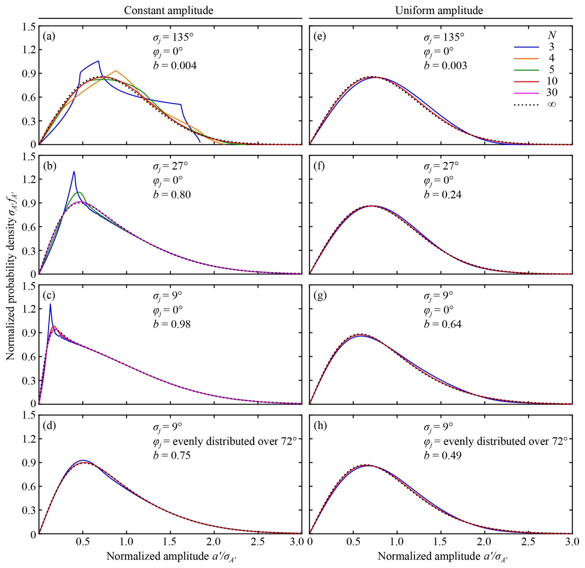
Figure 4 Convergence of the envelope-amplitude probability density function (PDF) $f_{A{}^{\prime }}$ with an increasing number of superimposed waves N. Amplitude variances of individual waves ${\mathit{\sigma }}_{A_j}$ are assumed to be equal. Left and right columns show PDFs under constant and uniform amplitude distributions, respectively. (a, e) PDFs for phase spread σ_j=135° and harmonic phase lag φ_j=0, (b, f) σ_j=27° and φ_j=0, (c, g) σ_j=9° and φ_j=0, and (d, h) σ_j=9° and φ_j distributed evenly over 72°. The b parameter of the generalized Rayleigh distribution, calculated from Eqs. (6) and (9d), is shown in each panel. Although not shown, the N=3 case with σ_j=9° and φ_j distributed evenly over 360° is practically given by the generalized Rayleigh distribution. In (a), distributions have maximum amplitudes of $a^{\prime }/{\mathit{\sigma }}_{A{}^{\prime }}\approx \mathrm{1.9}$, 2.2, and 2.4 for N=3, 4, and 5, respectively.

The results here suggest that, unless observed internal tides are dominantly generated at a few generation sites, nonharmonic internal tides are likely to have PDFs close to the limiting distributions in Eqs. (9a) and (9b) for the following three reasons: (i) it is unlikely that harmonic phase lags φ_j are close to each other because they depend, for example, on the distance and propagation speed between the sources and the observation location, (ii) relatively small phase spread is sufficient to approach the limiting distributions, and (iii) amplitude variability tends to increase the rate of convergence to the limiting distributions. If this is the case, the universality of the total PDFs would provide a convenient basis for observational data analysis and numerical modelling; however, it would also make the analysis of the underlying processes difficult because the total variance does not distinguish the separate contributions of individual wave components, and the total PDF (and the associated higher-order statistics) does not depend on the details of individual waves.

4.2 Observed time series, spectra, and energetics

The time series of harmonic and nonharmonic internal tides are shown in Fig. 3c–e. The VM1 isopycnal displacement amplitude ${\widehat{\mathit{\eta }}}_{\mathrm{1}}^{\mathrm{scaled}}\left(t\right)$ shows that the contributions of harmonic and nonharmonic internal tides are comparable at the PIL200 location (Fig. 3c). The harmonic internal tides show the spring–neap tidal cycle, but it is not clear in the nonharmonic counterpart. The envelope amplitudes of nonharmonic internal tides in the diurnal, semidiurnal, and quarter-diurnal frequency bands vary a lot without a stable mean, and the phases appear to be random (Fig. 3d and e). These features are consistent with the PDFs at the many source limit (Eqs. 9a and 9b) with a small b parameter. The results for the higher modes are similar, except that amplitudes decrease as the mode number increases, and the harmonic internal tides are substantially smaller than the nonharmonic counterpart (not shown).

Since the PIL200 location is on the continental shelf, there is a possibility that the local topographic excitation of higher modes by the barotropic mode or VM1 may lead to a similar behaviour of different modes. The visual inspection of the time series indeed showed intermittent periods when ${\widehat{\mathit{\eta }}}_n^{\mathrm{scaled}}\left(t\right)$ values for different modes were highly correlated. To check the influence of such correlation on nonharmonic internal-tide variance (the most important statistics considered in this study), the squared correlation coefficient matrix of the four modes of nonharmonic internal tides was calculated in the three frequency bands. The result shows that the off-diagonal components were mostly less than 5 %, except between semidiurnal VM2 and VM3 (20 %), semidiurnal VM2 and VM4 (10 %), semidiurnal VM3 and VM4 (21 %), and quarter-diurnal VM3 and VM4 (8 %). Therefore, the influence of the correlation is considered to be small overall, and the four modes are analysed separately in the following analyses.

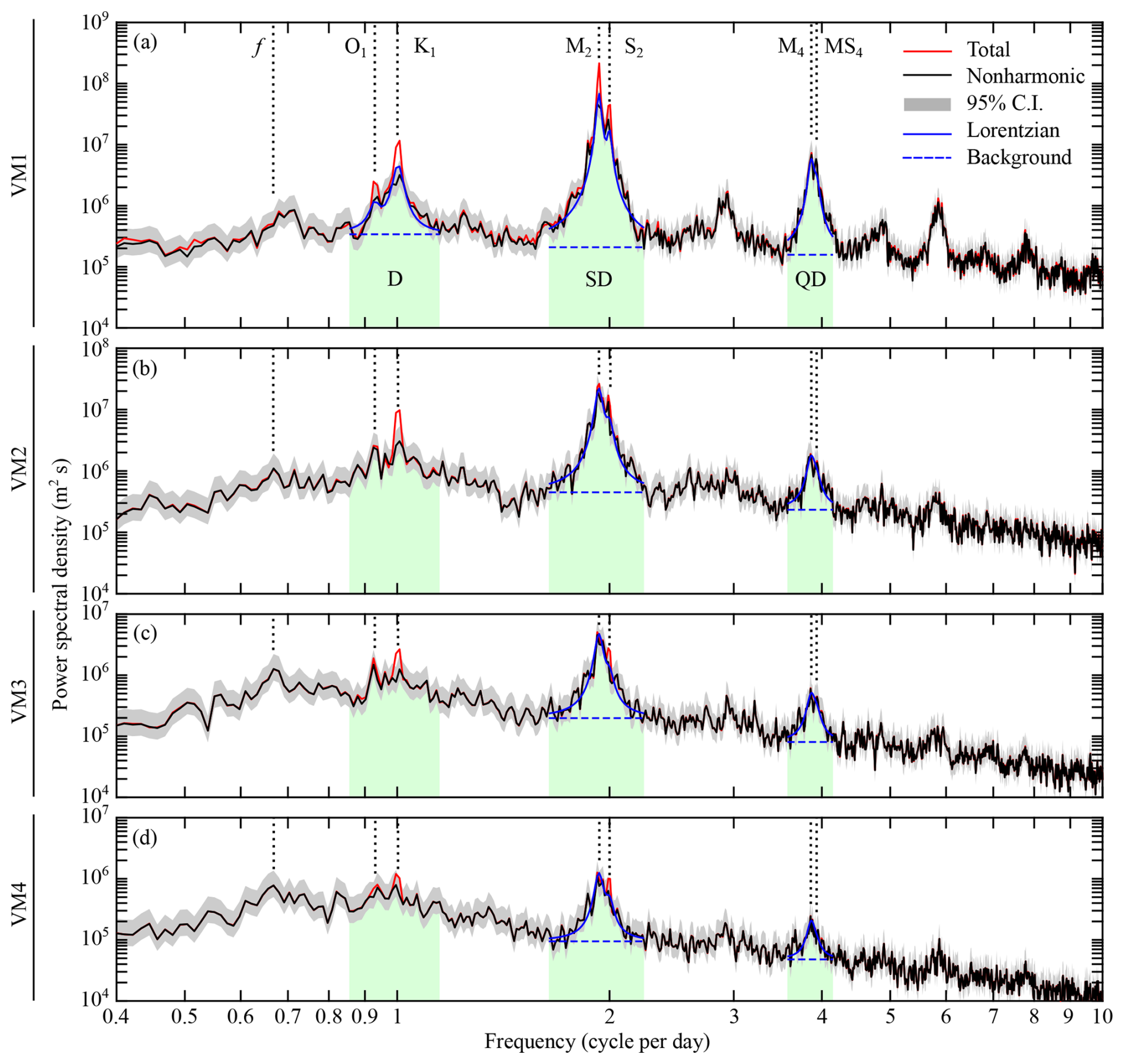
Figure 5 Power spectral density of the (scaled) isopycnal displacement amplitude of first four baroclinic modes. Grey shading shows the 95 % CI (confidence interval), and green shading shows frequency bands used to define the diurnal (D), semidiurnal (SD), and quarter-diurnal (QD) components, respectively. The blue solid and dashed lines show double Lorentzian spectra as in Eq. (19) and their background levels, respectively, from least-squares fitting.

The power spectral densities of the total and nonharmonic internal tides are shown in Fig. 5. The VM1 spectrum shows clear peaks at the diurnal, semidiurnal, and quarter-diurnal frequencies (Fig. 5a). The semidiurnal peak is tallest with M₂ being the dominant constituent. Since the PIL200 location is on the continental shelf, the quarter-diurnal (shallow water) internal tide is stronger than the diurnal internal tide. The subtraction of the harmonic tides reduces the heights of the peaks at the M₂, S₂, K₁, and O₁ frequencies but otherwise makes relatively small changes to the spectrum (compare red and black lines in Fig. 5a). The spectra of the higher-mode nonharmonic internal tides show clear peaks at the semidiurnal and quarter-diurnal frequencies, but the diurnal frequency band shows either an unclear peak or no peak (Fig. 5b–d).

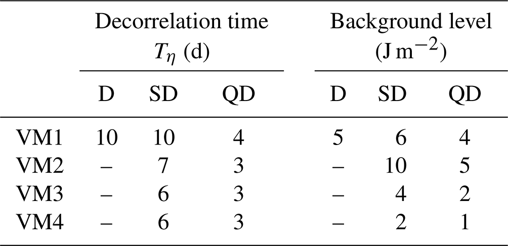
The spectra show the so-called “cusp” structure around the peaks. The bandpass filters used to separate the diurnal, semidiurnal, and quarter-diurnal components were chosen based on the widths of the corresponding cusps (green shading in Fig. 5). The spectral resolution is not high enough to resolve cusps around individual tidal constituents; however, it would be difficult to separate individual cusps in any case because the cusps are broader than the frequency differences among different constituents in the same frequency band. This provides the justification to use the diurnal, semidiurnal, and quarter-diurnal components in our analyses. The parameters associated with the cusps are shown in Table 1, and the results of least-squares fitting are shown in Fig. 5. The e-folding decorrelation times are 10, 6–10, and 3–4 d for the diurnal, semidiurnal, and quarter-diurnal band, respectively. These numbers are substantially smaller than those from satellite altimetry in the deep ocean (Zaron, 2022), but the causes are beyond the scope of this study. The decorrelation times were used to calculate the equivalent degrees of freedom of the nonharmonic internal-tide time series.

Table 1 Parameters estimated by least-squares fitting of the double Lorentzian model (Eq. 19) to cusps in power spectral density (Fig. 5). The background level S₀ in Eq. (19) is integrated over each frequency band so that the numbers can be directly compared to potential energies in Table 2. Abbreviations are as follows. VM: vertical mode, D: diurnal, SD: semidiurnal, and QD: quarter-diurnal.

The energetics in Table 2 show the following results. The nonharmonic-to-harmonic variance (or potential energy) ratio is about 1.1–1.2 for the VM1 diurnal and semidiurnal components (Table 2). The VM1 quarter-diurnal component is stronger than the diurnal component and dominantly nonharmonic. This is partly expected because the nonlinear interaction of harmonic–nonharmonic or nonharmonic–nonharmonic semidiurnal internal tides can generate a nonharmonic quarter-diurnal internal tide without the modulation processes. The VM2 semidiurnal internal tide has a nonharmonic-to-harmonic variance ratio of 6, and the topographic conversion of a nonharmonic VM1 semidiurnal internal tide would contribute to this large ratio. (These additional generation mechanisms are one of the major reasons why the terms “incoherent” or “non-phase-locked” tides are not used in this study.) Although the background variability seen in the PSD (Fig. 5) is included in these statistics, the comparisons of the background levels in Table 1 and the potential energies in Table 2 show that the errors are relatively small. The energy fluxes of nonharmonic VM1 and VM2 internal tides show propagation towards ESE–SE. The ratio of the total energy and energy flux suggests that roughly half of the energy is associated with directional waves for VM1 and VM2. Note that the uncertainties of the above mean values are relatively large for nonharmonic internal tides (about ±20 %–30 % for 95 % confidence intervals after more than 2 years of observations) because of the highly variable nature of nonharmonic internal tides.

Table 2 Vertically integrated energies (in J m⁻²) and energy fluxes (in W m⁻¹) of vertical-mode-one (VM1) and mode-two (VM2) internal tides in three frequency bands. The harmonic (H) components and mean (M) and standard deviation (SD) of nonharmonic (NH) components are calculated from harmonic analysis and bandpass-filtered time series, respectively.

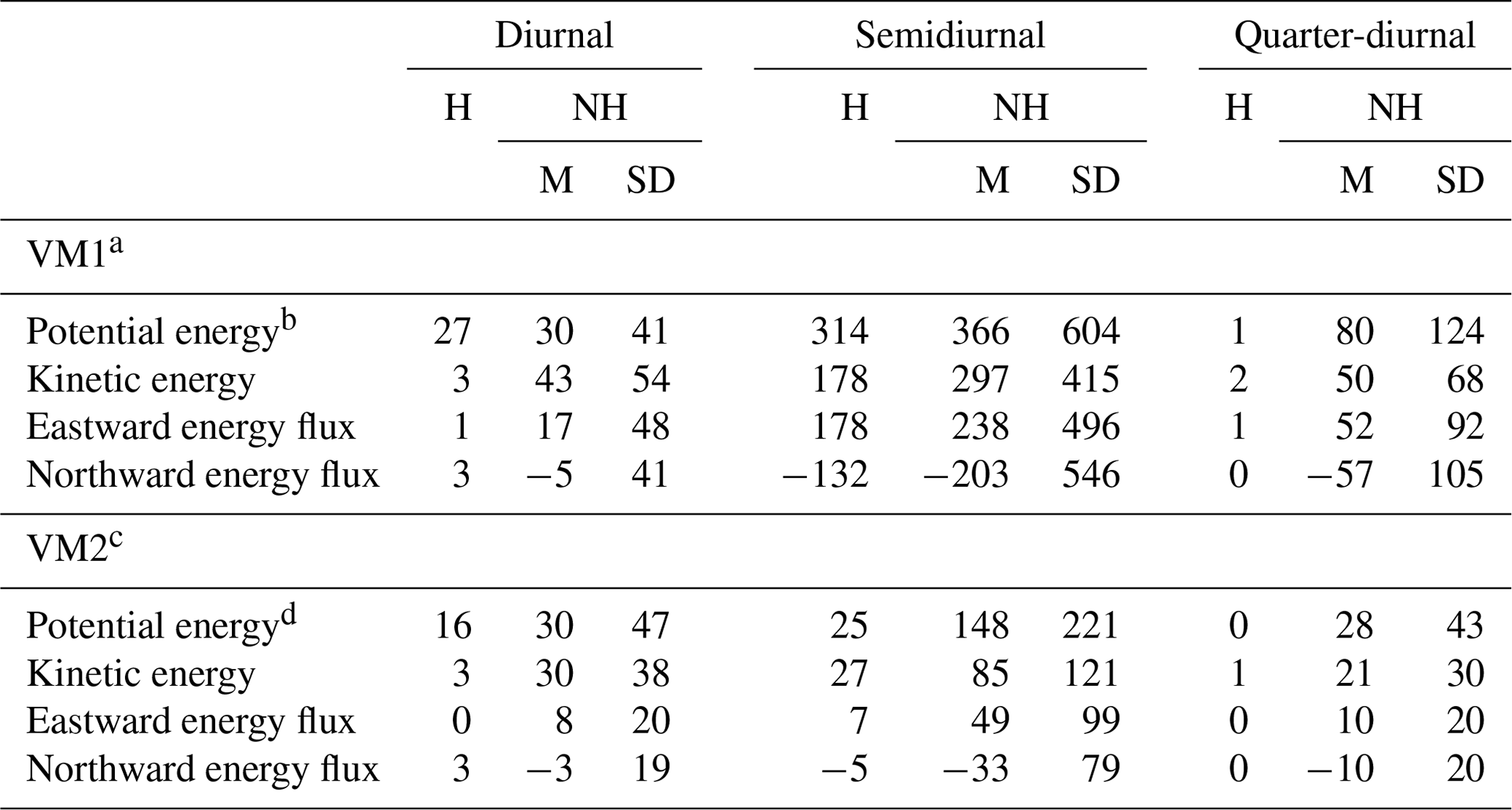
^a To calculate standard error, divide SD for diurnal, semidiurnal, and quarter-diurnal components by 8.7, 8.5, and 14, respectively. ^b Multiply by 0.12 to convert to variance of maximum isopycnal displacement within the water column and by $\mathrm{8.6}\times {\mathrm{10}}^{-\mathrm{8}}$ to that of surface displacement (neglecting seasonal cycle) (m²). ^c To calculate standard error, divide SD of semidiurnal and quarter-diurnal components by 11 and 16, respectively. ^d Multiply by 0.16 to convert to variance of extreme (minimum or maximum) isopycnal displacement within the water column (neglecting seasonal cycle) (m²).

4.3 Comparisons of observed and model probability density functions

The PDFs of the envelope amplitudes and phases of nonharmonic internal tides were calculated from the corresponding time series (Fig. 3d and e for VM1).

The comparisons of the observed and (fitted) model PDFs show that the limiting distributions (Eqs. 9a and 9b) provide a reasonable description of the amplitude and phase PDFs of the individual components of nonharmonic internal tides (Figs. 6 and 7). The estimated parameters are shown in the figure panels. Although the amplitude PDFs show some skewness, the phase PDFs suggest that the b parameter is small. The observed and model phase PDFs may appear to disagree in some cases because the observed phase PDFs were calculated as the marginal PDFs without amplitude weighting, but the model parameters were estimated based on the covariance matrix (Eq. 6), which takes amplitudes into account. However, the phase is roughly uniformly distributed (small b parameters) despite this difference. For more quantitative comparisons of the PDFs, the Pearson's χ² goodness-of-fit test shows that the observed distributions are not different from the limiting distributions at the 5 % significance level in all the cases in which the decorrelation time could be estimated from the cusp shapes (Figs. 6 and 7). These results show the applicability of the proposed statistical model to nonharmonic internal tides in the many source limit, at least for the available record length. Although the applicability is shown only at one location in this study, the convergence rate of the PDFs, shown in the previous section, suggests that the proposed statistical model has wide applicability to nonharmonic internal tides, regardless of the details of underlying physical processes. The applicability to different frequency bands and different modes, which are likely to have different generation processes, supports this speculation. (The six cases in Figs. 6 and 7 are shown to demonstrate this point, although the results look rather similar.)

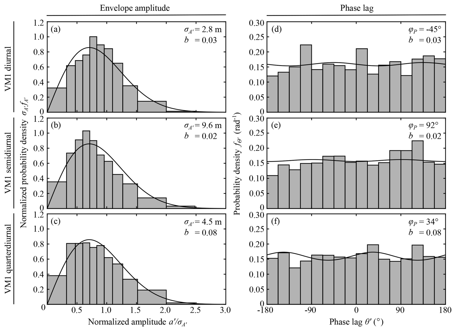
Figure 6 Comparisons of envelope-amplitude and phase probability density functions from the statistical model and PIL200 observations for nonharmonic vertical-mode-one internal tides. (a–c) Envelope amplitude, (d–f) phase lag. Upper, middle, and bottom rows show diurnal, semidiurnal, and quarter-diurnal components, respectively. Solid lines show distributions in the “many source” limit, with estimated model parameters shown in each panel.

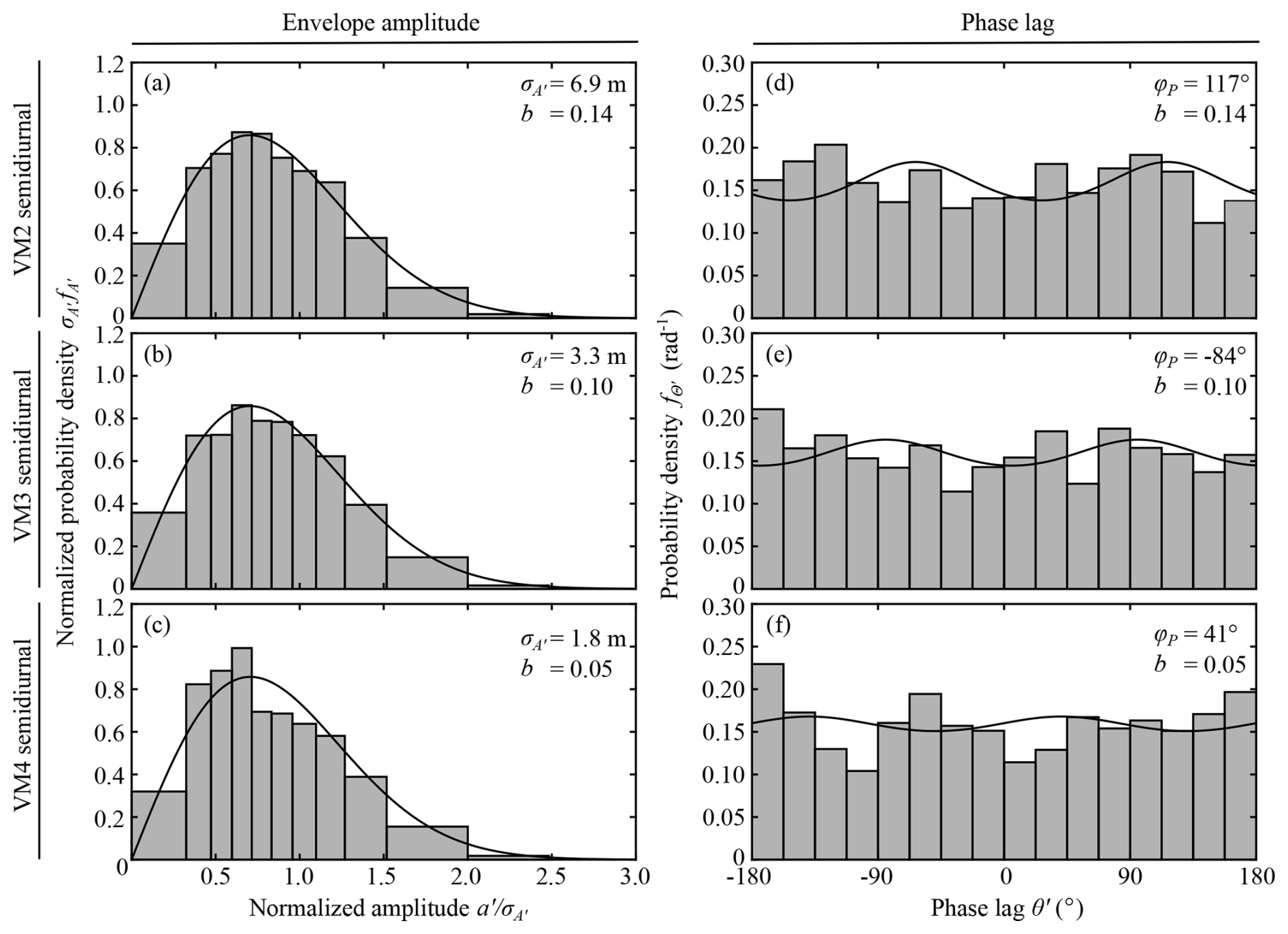
Figure 7 Comparisons of envelope-amplitude and phase probability density functions from the statistical model and PIL200 observations for semidiurnal frequency band. (a–c) Envelope amplitude, (d–f) phase lag. Upper, middle, and bottom rows: vertical mode two (VM2), mode three (VM3), and mode four (VM4), respectively. Solid lines show distributions in the “many source” limit, with estimated model parameters shown in each panel.

5 Discussion

The major novel contributions of this paper are deriving the PDFs of nonharmonic internal tides, observationally showing their applicability, and demonstrating the importance of viewing nonharmonic internal tides as the superposition of many random waves. These contributions were made by developing a statistical model of nonharmonic or incoherent internal tides observed at a fixed location from similar models developed in other fields of physics and engineering (e.g. Barakat, 1974, 1988; Abdi et al., 2000) and by comparing the results with the PIL200 observations. An important aspect of the statistical model is allowing non-uniform and non-identical probability distributions for individual wave components, which enables application to spatially distributed sources and increasing phase randomness with distance from the observation location.

Once the above view is adopted, some of the results of this paper might appear trivial because it follows from the central limit theorem in statistics; however, the above view was not adopted in the previous studies of nonharmonic internal tides in a quantitative manner. A demonstration of this is the following simple model for internal tides, used by Colosi and Munk (2006), Zaron (2015), Geoffroy and Nycander (2022), and Kachelein et al. (2024):

$$\begin{array}{}\text{(21)}& {\widehat{\mathit{\eta }}}_{\mathrm{1}}=(r+A^{\prime })e^{i\left({\mathit{\omega }}_{\mathrm{0}}t-\mathrm{\Theta }\right)}.\end{array}$$

Here, the subscript 0 is added to ω to emphasize that it is the fixed angular frequency of a harmonic tide, r is the amplitude of the harmonic internal tide, and A^′ and Θ are random amplitude and phase, respectively, which are assumed to be Gaussian. (Although ${\widehat{\mathit{\eta }}}_{\mathrm{1}}$ is hereafter a random variable, it is written in lowercase.) This model essentially assumes a single sinusoidal wave whose amplitude and phase are modulated by random processes, as the proposed statistical model assumes for individual wave components. However, when a nonharmonic internal tide results from the superposition of many random waves, the PDF becomes joint Gaussian in Cartesian coordinates (see Fig. 8a or grey dots in Fig. 1 for samples from the PIL200 observations), which can be quite different from the PDF associated with the above model (i.e. A^′ and Θ are joint Gaussian in polar coordinates). The difference could be relatively minor when Var(A^′) and Var(Θ) are small (Fig. 8b) but substantial when Var(Θ) is not small (Fig. 8c). In particular, the above model has two awkward features when the peak of the PDF is located within a few standard deviations of the origin. First, the phase of a nonharmonic internal tide can be almost uniformly distributed as seen in the right column of Figs. 6 and 7; however, the above model becomes awkward when Var(Θ) is larger than about 1 because the “wrapping” of phase is not included when the phase spread is beyond the full period 2π. Second, when the PDF is seen in Cartesian coordinates, the PDF has a peak near the origin because the radial Gaussian distribution must be divided by the radius upon conversion to Cartesian coordinates to impose Eq. (5). The peak near the origin becomes wider as Var(A^′) increases. Since such a peak is unrealistic for a nonharmonic internal tide, Var(A^′) effectively has a relatively small upper limit of roughly 0.1r. Figure 8c shows the PDF as broad as possible under these constraints. It is worth noting that Var(A^′) and Var(Θ) estimated from observations in the previous studies (Colosi and Munk, 2006; Geoffroy and Nycander, 2022) are almost at these upper limits, and the observed distributions in Fig. 11 of Colosi and Munk (2006) appear closer to Fig. 8a than Fig. 8c.

Figure 8 Comparison of probability density functions (PDFs) under simple (or “toy”) models. (a) PDF under Eq. (22), (b) PDF under Eq. (21) with relatively small Var(A^′) and Var(Θ), and (c) that under relatively large Var(A^′) and Var(Θ). The parameters used are shown in each panel.

The results of this paper suggest that the many source limit is common in nonharmonic internal tides, and hence it is important to construct an alternative simple model that is applicable to the joint Gaussian distribution in Cartesian coordinates. This can be done easily. Since the complex amplitude $X^{\prime }+i{Y}^{\prime }$ has the joint Gaussian distribution, it appears most convenient to rotate the coordinates so that the resultant amplitudes $X{}_{\mathrm{P}}^{\prime }$ and $Y{}_{\mathrm{P}}^{\prime }$ are uncorrelated. Then, the most straightforward simple model is

$$\begin{array}{}\text{(22)}& {\widehat{\mathit{\eta }}}_{\mathrm{1}}=r{e}^{i\left({\mathit{\omega }}_{\mathrm{0}}t-\mathit{\phi }\right)}+\left(X{}_{\mathrm{P}}^{\prime }+iY{}_{\mathrm{P}}^{\prime }\right)e^{i\left({\mathit{\omega }}_{\mathrm{0}}t-\mathit{\phi }{}_{\mathrm{P}}^{\prime }\right)},\end{array}$$

where $\mathit{\phi }{}_{\mathrm{P}}^{\prime }$ is the angle of the rotated $x_{\mathrm{P}}^{\prime }$ axis on the complex plane. This model is convenient because $X_{\mathrm{P}}^{\prime }$ and $Y_{\mathrm{P}}^{\prime }$ are independent Gaussian variables with zero mean, and it can deal with uniform phase distribution within the Gaussian assumption. Considering the real part of the above expression, the auto-covariance function is

$$\begin{array}{}\text{(23)}& C_{\mathit{\eta }}\left(\mathit{\tau }\right)={\displaystyle \frac{\mathrm{1}}{\mathrm{2}}}\left\{r^{\mathrm{2}}+\left(C_{X{}_{\mathrm{P}}^{\prime }}\left(\mathit{\tau }\right)+C_{Y{}_{\mathrm{P}}^{\prime }}\left(\mathit{\tau }\right)\right)\right\}\cos {\mathit{\omega }}_{\mathrm{0}}\mathit{\tau },\end{array}$$

where τ is the time lag, and $C_{X{}_{\mathrm{P}}^{\prime }}$ and $C_{Y{}_{\mathrm{P}}^{\prime }}$ are the auto-covariance functions of $X_{\mathrm{P}}^{\prime }$ and $Y_{\mathrm{P}}^{\prime }$, respectively. Following the previous studies (Colosi and Munk, 2006; Geoffroy and Nycander, 2022), we assume $C_{X{}_{\mathrm{P}}^{\prime }}\left(\mathit{\tau }\right)={\mathit{\sigma }}_{X_{\mathrm{P}}}^{\mathrm{2}}{e}^{-\left|\mathit{\tau }\right|/T_{\mathit{\eta }}}$ and $C_{Y{}_{\mathrm{P}}^{\prime }}\left(\mathit{\tau }\right)={\mathit{\sigma }}_{Y_{\mathrm{P}}}^{\mathrm{2}}{e}^{-\left|\mathit{\tau }\right|/T_{\mathit{\eta }}}$, where T_η is the e-folding decorrelation time. Then, the Fourier transform of C_η and appropriate scaling yield the (one-sided) power spectral density:

$$\begin{array}{}\text{(24)}& \begin{array}{rl}& S_{\mathit{\eta }}\left(\mathit{\omega }\right)={\displaystyle \frac{\mathrm{1}}{\mathrm{2}}}{r}^{\mathrm{2}}\mathit{\delta }\left(\mathit{\omega }-{\mathit{\omega }}_{\mathrm{0}}\right)+{\displaystyle \frac{{\mathit{\sigma }}_{A^{\prime }}^{\mathrm{2}}}{\mathrm{2}\mathit{\pi }{T}_{\mathit{\eta }}}}\\ & \times \left({\displaystyle \frac{\mathrm{1}}{{\left(\mathit{\omega }-{\mathit{\omega }}_{\mathrm{0}}\right)}^{\mathrm{2}}+T_{\mathit{\eta }}^{-\mathrm{2}}}}+{\displaystyle \frac{\mathrm{1}}{{\left(\mathit{\omega }+{\mathit{\omega }}_{\mathrm{0}}\right)}^{\mathrm{2}}+T_{\mathit{\eta }}^{-\mathrm{2}}}}\right),\end{array}\end{array}$$

where Eq. (9c) is used. The last term is often omitted assuming ω₀T_η≫1 but is mathematically required for one-sided spectra (i.e. only positive ω is considered). As seen in these expressions, Eq. (22) leads to a much simpler formula of power spectral density than Eq. (21) (see the derivation in Colosi and Munk, 2006).

Some readers may think that simple models such as Eqs. (21) and (22) are merely a toy model; however, the details can be important because Eq. (21) has been used for the quantitative estimation of parameters associated with nonharmonic internal tides. For example, Geoffroy and Nycander (2022) used the auto-covariance function of Eq. (21) to estimate the variance of nonharmonic internal tides from global Argo data. Another example is the estimates of the decorrelation time T_η from satellite altimetry by Zaron (2015, 2022). Zaron (2022) fitted the Lorentzian spectrum in Eq. (24) to the power spectrum of the sea level anomaly, although he assumed a Gaussian phase variation that does not yield the Lorentzian spectrum in general (see Colosi and Munk, 2006). If the observed nonharmonic internal tides are approximately in the many source limit, the proposed simple model and Eq. (24) would provide justification for his choice. These parameters provide important bases for distinguishing quasi-geostrophic (or “balanced”) currents and internal tides in wide-swath altimeter data, such as those from the Surface Water and Ocean Topography (SWOT) mission (Morrow et al., 2019).

Note that the proposed statistical model is also applicable to a small number of wave sources (see Appendix A), although this paper focused on the many source limit. It would be interesting to make comparisons in regions affected by a few strong sources in the future, such as around Hawaii and the French Polynesian Islands (e.g. Zaron and Egbert, 2014; Buijsman et al., 2017).

Since a PDF is basic information that characterize a stochastic process, the PDFs proposed in this study can be used for many purposes in the future. For example, for surface waves, the PDF of wave amplitude is used for many engineering applications (e.g. Horikawa, 1978). Similarly, the proposed PDF can be used to assess the risk of infrequent strong waves for offshore operations. Another example would be the occurrence of nonlinear internal bores and solitary waves, which develop from internal tides. On the shallow continental shelf off California where these nonlinear waves occur regularly, Colosi et al. (2018) reported that the energy flux of internal bores and solitary waves follows the exponential distribution. If the proposed envelope-amplitude PDF is applicable to a deeper location before these nonlinear waves develop, it would allow us to investigate the statistical relationship between these nonlinear waves and the underlying internal tides.

If the many source limit is common for nonharmonic internal tides as suggested in this paper, one of the most important problems would be to understand what controls the variance of nonharmonic internal tides because the covariance matrix in Eq. (6) determines the PDF (and the associated higher-order statistics). Although the proposed statistical model includes some parameters pertaining to this point, such as the strengths of the sources and the phase spread, the comparisons with the PIL200 observations unfortunately did not provide such information. This is actually expected for any cases in which the observed PDF is close to the limiting distribution because the total variance does not distinguish the separate contributions of individual wave components, and the PDF does not depend on the details of the individual waves or the underlying physical processes. For example, the phase of observed nonharmonic internal tides can be nearly uniformly distributed when the phases of individual wave components vary less than 5 % (of the total 2π), and the observed amplitude tends to show large variability when the amplitudes of individual components do not vary at all. More broadly, this situation appears to be common for a system with large degrees of freedom, as statistical mechanics show that statistical principles make a macroscopic quantity not necessarily sensitive to the details of microscopic processes (e.g. Reif, 1965). For process-based understanding, Part 2 of this study (Shimizu, 2025) combines the proposed statistical model with adjoint and stochastic models, which provide spatially distributed source strengths and phase spread, respectively. Then, the model suite enables us to investigate important processes and parameters controlling nonharmonic internal-tide variance.

6 Conclusions

This paper developed a statistical model of nonharmonic or incoherent internal tides and compared the model probability density functions (PDFs) with the observed PDFs at the PIL200 location on the Australian North West Shelf. To my knowledge, this is the first study that focused on the statistical aspects of nonharmonic internal tides and considered the importance of viewing nonharmonic internal tides as the superposition of many random waves. The major new findings of this paper are as follows.

• The PDF of complex-valued nonharmonic internal-tide amplitude approaches the joint Gaussian distribution on the complex plane as the number of independent wave sources increases. The corresponding envelope-amplitude PDF is a generalization of the Rayleigh distribution.

• Under conditions that are likely for nonharmonic internal tides, the convergence to the “many source” limit is relatively fast. It requires about 10 independent sources in most situations and as few as three in favourable situations. This implies that nonharmonic internal tides tend to have universal PDFs.

• The observed PDFs were not different from the limiting distributions for nonharmonic vertical-mode-one to mode-four internal tides in the diurnal, semidiurnal, and quarter-diurnal frequency bands at the 5 % significance level, provided that the power spectra show the corresponding tidal peaks clearly. This observationally shows the applicability of the proposed PDFs in the many source limit.

• The convergence to the universal PDFs unfortunately makes process investigation based on observations more difficult because the total variance does not distinguish the separate contributions of individual wave sources, and the PDFs become insensitive to the details of individual waves or the underlying physical processes.

Also, the statistical model was used to revise the common simple (or “toy”) model of internal tides that has been used for observational data analysis so that it is applicable to the many source limit. Since the last point above makes process investigation difficult, Part 2 of this study (Shimizu, 2025) develops a new modelling framework and model suite to investigate important processes and parameters controlling nonharmonic internal-tide variance based on the proposed statistical model.

Appendix A: Calculation of probability density function for an arbitrary number of wave sources

This Appendix describes the general version of the statistical model in Sect. 2.1 applicable to arbitrary N. The standard approach in statistics to derive the PDF of a sum of random variables consists of (i) considering the joint probability density function (PDF) of individual components, (ii) calculating the characteristic function (i.e. the Fourier transform of the PDF) of each component, (iii) taking the product of the characteristic functions, and (iv) calculating the total PDF as the inverse Fourier transform of the total characteristic function. Because there are some pitfalls to deal with PDFs in polar coordinates, such as Eq. (5), the derivation below starts from the expression in Cartesian coordinates, although the results are written in polar coordinates. Please refer to Appendix B for a brief summary of the coordinate transformation and Fourier and Hankel transform pairs in Cartesian and polar coordinates used in this paper.

The derivation of PDFs proceeds as follows. To calculate the characteristic function ϕ_j, we consider the PDF of ($X_j^{\prime }$, $Y_j^{\prime }$), define ϕ_j as the two-dimensional (2D) Fourier transform of $f_{X{}_j^{\prime }Y{}_j^{\prime }}$, and then convert the expression to its polar counterpart (A_j, Θ_j). The characteristic function in Cartesian coordinates is

$$\begin{array}{}\text{(A1a)}& {\displaystyle }\begin{array}{rl}{\mathit{\varphi }}_j& \left({\mathit{\kappa }}_x,{\mathit{\kappa }}_y\right)=\underset{-\mathrm{\infty }}{\overset{\mathrm{\infty }}{\int }}\underset{-\mathrm{\infty }}{\overset{\mathrm{\infty }}{\int }}{f}_{X{}_j^{\prime }Y{}_j^{\prime }}\left(x_j^{\prime },y_j^{\prime }\right)e^{i\left({\mathit{\kappa }}_x{x}_j^{\prime }+{\mathit{\kappa }}_y{y}_j^{\prime }\right)}\mathrm{d}{x}_j^{\prime }\mathrm{d}{y}_j^{\prime }\\ & =e^{-i{\mathrm{\Delta }}_j}\underset{-\mathrm{\infty }}{\overset{\mathrm{\infty }}{\int }}\underset{-\mathrm{\infty }}{\overset{\mathrm{\infty }}{\int }}{f}_{X_j{Y}_j}\left(x_j,y_j\right)e^{i\left({\mathit{\kappa }}_x{x}_j+{\mathit{\kappa }}_y{y}_j\right)}\mathrm{d}{x}_j\mathrm{d}{y}_j,\end{array}\text{(A1b)}& {\displaystyle }\begin{array}{rl}& {\mathrm{\Delta }}_j={\mathit{\kappa }}_x{\stackrel{\mathrm{‾}}{x}}_j+{\mathit{\kappa }}_y{\stackrel{\mathrm{‾}}{y}}_j,\end{array}\end{array}$$

where (${\stackrel{\mathrm{‾}}{x}}_j,{\stackrel{\mathrm{‾}}{y}}_j)=(\mathrm{E}\left(x_j\right),\mathrm{E}\left(y_j\right)$), (κ_x, κ_y) is the “wavenumber” vector used in Fourier transform, Δ_j is the phase shift originating from the subtraction of the mean in Eq. (2), and $f_{X_j^{\prime }{Y}_j^{\prime }}(x_j^{\prime },y_j^{\prime })=f_{X_j^{\prime }{Y}_j^{\prime }}(x_j-{\stackrel{\mathrm{‾}}{x}}_j,y_j-{\stackrel{\mathrm{‾}}{y}}_j)=f_{X_j{Y}_j}(x_j,y_j)$ is used. The conversion to polar coordinates is done using Eq. (1) and $({\mathit{\kappa }}_x,{\mathit{\kappa }}_y)=\mathit{\kappa }(\cos \mathit{\lambda },\sin \mathit{\lambda })$. Then, Eqs. (A1a) and (A1b) become

$$\begin{array}{}\text{(A2a)}& {\displaystyle }& {\displaystyle }{\mathit{\varphi }}_j(\mathit{\kappa },\mathit{\lambda })=e^{-i{\mathrm{\Delta }}_j}\underset{-\mathit{\pi }}{\overset{\mathit{\pi }}{\int }}\underset{\mathrm{0}}{\overset{\mathrm{\infty }}{\int }}{f}_{A_j{\mathrm{\Theta }}_j}\left(a_j,{\mathit{\theta }}_j\right)e^{i\mathit{\kappa }{a}_j\cos \left(\mathit{\lambda }+{\mathit{\theta }}_j\right)}\mathrm{d}{a}_j\mathrm{d}{\mathit{\theta }}_j,\text{(A2b)}& {\displaystyle }& {\displaystyle }{\mathrm{\Delta }}_j=\mathit{\kappa }{r}_j\cos \left(\mathit{\lambda }+{\mathit{\phi }}_j\right).\end{array}$$

Although the PDF including the mean ($f_{A_j{\mathrm{\Theta }}_j}$) appears in this equation, the characteristic function is defined for deviation from the mean, as in the original expression in Eqs. (A1a) and (A1b) because of the phase shift operator $e^{-i{\mathrm{\Delta }}_j}$. The total characteristic function is given by

$$\begin{array}{}\text{(A3)}& \mathit{\varphi }=\prod _{j=\mathrm{1}}^N{\mathit{\varphi }}_j.\end{array}$$

The total PDF is given by the inverse Fourier transform of ϕ. We consider the inverse 2D Fourier transform in Cartesian coordinates first and then transform the coordinates to polar coordinates. The expression in Cartesian coordinates is given by Eq. (B1b) but with f_XY and (x, y) replaced by $f_{X^{\prime }{Y}^{\prime }}$ and (x^′, y^′), respectively. The corresponding expression in polar coordinates is

$$\begin{array}{}\text{(A4)}& \begin{array}{rl}{f}_{A^{\prime }{\mathrm{\Theta }}^{\prime }}(a,\mathit{\theta })& ={\displaystyle \frac{a}{(\mathrm{2}\mathit{\pi }{)}^{\mathrm{2}}}}\underset{-\mathit{\pi }}{\overset{\mathit{\pi }}{\int }}\underset{\mathrm{0}}{\overset{\mathrm{\infty }}{\int }}\mathit{\varphi }(\mathit{\kappa },\mathit{\lambda })e^{-i\mathit{\kappa }a\cos (\mathit{\lambda }+\mathit{\theta })}\mathit{\kappa }\mathrm{d}\mathit{\kappa }\mathrm{d}\mathit{\lambda },\\ & ={\displaystyle \frac{a}{\mathrm{2}\mathit{\pi }}}\sum _{k=-\mathrm{\infty }}^{\mathrm{\infty }}(-i{)}^k{e}^{-ik\mathit{\theta }}\underset{\mathrm{0}}{\overset{\mathrm{\infty }}{\int }}{\mathit{\varphi }}^{\left(k\right)}(\mathit{\kappa }\left)J_k\right(\mathit{\kappa }a)\mathit{\kappa }\mathrm{d}\mathit{\kappa },\end{array}\end{array}$$

where J_k is the Bessel function of the first kind of the order k, and the factor a is multiplied to impose Eq. (5) upon conversion to polar coordinates. The second expression is obtained using the azimuthal Fourier series in Eq. (B4a) (with ϕ^(k) being the Fourier coefficients) and the properties of the Bessel function (Abramowitz and Stegun, 1972, Eqs. 9.1.5, 21, and 35 or DLMF, 2025, Eqs. 10.4.1, 10.9.2, and 10.11.1). Note that this total PDF is for the deviation from the mean as in Eq. (3), although the PDFs of each component $f_{A_j{\mathrm{\Theta }}_j}$ in Eq. (A2a) include the mean. The radial (or envelope-amplitude) PDF is given by the marginal probability:

$$\begin{array}{}\text{(A5)}& \begin{array}{rl}{f}_{A^{\prime }}\left(a\right)& =\underset{-\mathit{\pi }}{\overset{\mathit{\pi }}{\int }}{f}_{A^{\prime }{\mathrm{\Theta }}^{\prime }}(a,\mathit{\theta })\mathrm{d}\mathit{\theta }\\ & =a\underset{\mathrm{0}}{\overset{\mathrm{\infty }}{\int }}{\mathit{\varphi }}^{\left(\mathrm{0}\right)}\left(\mathit{\kappa }\right)J_{\mathrm{0}}\left(\mathit{\kappa }a\right)\mathit{\kappa }\mathrm{d}\mathit{\kappa }.\end{array}\end{array}$$

If A_j has an upper limit α_j, the computational load of the Hankel transform in Eq. (A4) and the subsequent moments can be reduced (Bennett, 1948; Barakat, 1974, 1988). This is because A^′ has the maximum value (see Fig. 1):

$$\begin{array}{}\text{(A6)}& R=\sum _{j=\mathrm{1}}^N|{\mathit{\alpha }}_j+r_j|.\end{array}$$

Since the PDF is zero for a>R, the Hankel transform in Eq. (A4) can be replaced by the Fourier–Bessel series of the form

$$\begin{array}{}\text{(A7)}& f_{A^{\prime }{\mathrm{\Theta }}^{\prime }}(a,\mathit{\theta })={\displaystyle \frac{a}{\mathrm{2}\mathit{\pi }R}}\sum _{k=-\mathrm{\infty }}^{\mathrm{\infty }}{e}^{-ik\mathit{\theta }}\sum _{l=\mathrm{1}}^{\mathrm{\infty }}{\mathit{\alpha }}_{k,l}{J}_k\left({\displaystyle \frac{j_{k,l}a}{R}}\right),\end{array}$$

where j_k,l is the lth root of J_k, and α_k,l represents the amplitudes of individual components (to be determined). The Fourier–Bessel series is a generalized Fourier series using Bessel functions as the basis functions (instead of trigonometric functions). It often appears as a part of two-dimensional Fourier transform in polar coordinates. Assuming azimuthal Fourier series,

$$\begin{array}{}\text{(A8)}& f_{A^{\prime }{\mathrm{\Theta }}^{\prime }}(a,\mathit{\theta })={\displaystyle \frac{\mathrm{1}}{\mathrm{2}\mathit{\pi }}}\sum _{k=-\mathrm{\infty }}^{\mathrm{\infty }}{f}_{A^{\prime }}^{\left(k\right)}\left(a\right)e^{-ik\mathit{\theta }},\end{array}$$

the amplitudes α_k,l are obtained using the orthogonality of the Bessel function over a fixed interval (Abramowitz and Stegun, 1972, Eq. 11.4.5 or DLMF, 2025, Eq. 10.22.37):

$$\begin{array}{}\text{(A9)}& \underset{\mathrm{0}}{\overset{R}{\int }}a{J}_k\left(j_{k,l}{\displaystyle \frac{a}{R}}\right)J_k\left(j_{k,m}{\displaystyle \frac{a}{R}}\right)\mathrm{d}a={\displaystyle \frac{R^{\mathrm{2}}}{\mathrm{2}}}{J}_{k+\mathrm{1}}{\left(j_{k,l}\right)}^{\mathrm{2}}{\mathit{\delta }}_{l,m},\end{array}$$

where δ_l,m is the Kronecker delta. The resultant amplitudes are

$$\begin{array}{}\text{(A10)}& {\mathit{\alpha }}_{k,l}={\displaystyle \frac{\mathrm{2}}{R{J}_{k+\mathrm{1}}^{\mathrm{2}}\left(j_{k,l}\right)}}\underset{\mathrm{0}}{\overset{R}{\int }}{f}_{A^{\prime }}^{\left(k\right)}\left(a\right)J_k\left(j_{k,l}{\displaystyle \frac{a}{R}}\right)\mathrm{d}a.\end{array}$$

However, since $f_{A^{\prime }}^{\left(k\right)}\left(a\right)$ is zero for a>R, the integral can be related to ϕ^(k) through the Hankel transform of $f_{A^{\prime }}^{\left(k\right)}\left(a\right)$ (compare the above integral with Eq. B6 in Appendix B). So, α_k,l can be written as

$$\begin{array}{}\text{(A11)}& {\mathit{\alpha }}_{k,l}=(-i{)}^k{\displaystyle \frac{\mathrm{2}}{R{J}_{k+\mathrm{1}}^{\mathrm{2}}\left(j_{k,l}\right)}}{\mathit{\varphi }}^{\left(k\right)}\left({\displaystyle \frac{j_{k,l}}{R}}\right).\end{array}$$

Substituting this into Eq. (A7) yields the Fourier–Bessel version of Eq. (A4). The advantage of the Fourier–Bessel solution is that, unlike Eq. (A4), Eq. (A7) requires the evaluation of ϕ^(k) only at discrete points. Then, the mean square amplitude is given by

$$\begin{array}{}\text{(A12)}& \begin{array}{rl}E\left(A{{}^{\prime }}^{\mathrm{2}}\right)& =\underset{\mathrm{0}}{\overset{\mathrm{\infty }}{\int }}{a}^{\mathrm{2}}{f}_{A^{\prime }}\left(a\right)\mathrm{d}a=\mathrm{4}{R}^{\mathrm{2}}\sum _{l=\mathrm{1}}^{\mathrm{\infty }}{\displaystyle \frac{\mathrm{1}}{j_{\mathrm{0},l}^{\mathrm{2}}{J}_{\mathrm{1}}{\left(j_{\mathrm{0},l}\right)}^{\mathrm{2}}}}\\ & \times \left(J_{\mathrm{0}}\left(j_{\mathrm{0},l}\right)+\left({\displaystyle \frac{j_{\mathrm{0},l}}{\mathrm{2}}}-{\displaystyle \frac{\mathrm{2}}{j_{\mathrm{0},l}}}\right)J_{\mathrm{1}}\left(j_{\mathrm{0},l}\right)\right){\mathit{\varphi }}^{\left(\mathrm{0}\right)}\left({\displaystyle \frac{j_{\mathrm{0},l}}{R}}\right).\end{array}\end{array}$$

The components of the covariance matrix Eq. (6) are given by

$$\begin{array}{}\text{(A13a)}& {\displaystyle }& {\displaystyle }{\mathit{\sigma }}_X^{\mathrm{2}}={\displaystyle \frac{\mathrm{1}}{\mathrm{2}}}E\left(A{{}^{\prime }}^{\mathrm{2}}\right)-Re\left(B\right),\text{(A13b)}& {\displaystyle }& {\displaystyle }{\mathit{\sigma }}_Y^{\mathrm{2}}={\displaystyle \frac{\mathrm{1}}{\mathrm{2}}}E\left(A{{}^{\prime }}^{\mathrm{2}}\right)+Re\left(B\right),\text{(A13c)}& {\displaystyle }& {\displaystyle }{\mathit{\rho }}_{XY}={\displaystyle \frac{\mathrm{1}}{{\mathit{\sigma }}_X{\mathit{\sigma }}_Y}}\mathrm{Im}\left(B\right),\text{(A13d)}& {\displaystyle }& {\displaystyle }B=R^{\mathrm{2}}\sum _{l=\mathrm{1}}^{\mathrm{\infty }}{\displaystyle \frac{\mathrm{1}}{j_{\mathrm{2},l}{J}_{\mathrm{3}}\left(j_{\mathrm{2},l}\right)}}{\mathit{\varphi }}^{\left(\mathrm{2}\right)}\left({\displaystyle \frac{j_{\mathrm{2},l}}{R}}\right).\end{array}$$

To calculate the PDF and covariance under the wrapped normal phase distribution in Eq. (12), the characteristic function of each component is needed. It is given by substituting Eqs. (11) and (12) into Eq. (A2a) and evaluating the integral. The result is

$$\begin{array}{}\text{(A14)}& \begin{array}{rl}{\mathit{\varphi }}_j(\mathit{\kappa },\mathit{\lambda })=& e^{-i{\mathrm{\Delta }}_j}\sum _{k=-\mathrm{\infty }}^{\mathrm{\infty }}{i}^k{e}^{-k^{\mathrm{2}}{\mathit{\sigma }}_j^{\mathrm{2}}/\mathrm{2}}{e}^{ik\left(\mathit{\lambda }+{\mathit{\phi }}_j\right)}\\ & \times \underset{\mathrm{0}}{\overset{\mathrm{\infty }}{\int }}{f}_{A_j}\left(a_j\right)J_k\left(\mathit{\kappa }{a}_j\right)\mathrm{d}{a}_j,\end{array}\end{array}$$

where Δ_j is defined in Eq. (A2b). This is substituted into Eq. (A3) to calculate PDFs and moments.

Using the above theory, the PDFs in Fig. 4 were calculated as follows. The azimuthal Fourier coefficients ϕ^(k) in Eqs. (A12) and (A13d) for k=0, 2 and radial integration in Eq. (A14) were calculated numerically. The PDFs and covariance matrices were calculated in the Fourier–Bessel series using Eqs. (A7)–(A13a–A13d). It is worth noting that, for large N, the majority of $f_{A^{\prime }{\mathrm{\Theta }}^{\prime }}$ values tend to be located in a much smaller area near the origin compared to the whole non-zero area. For example, the PDF of the generalized Rayleigh distribution becomes small for $a>\mathrm{3}{\mathit{\sigma }}_{A^{\prime }}$. In such cases, $f_{A^{\prime }{\mathrm{\Theta }}^{\prime }}$ excluding the tail can be evaluated with reduced R from Eq. (A6), which can provide substantial reduction of the computational cost with a relatively small loss of accuracy. In this paper, $R=\mathrm{4}{\mathit{\sigma }}_{A^{\prime }}$ is used for computational efficiency.

It is also worth noting that the convergence of the Fourier–Bessel series solution was slow when the PDF contained singularities, peaks, or edges. With the above choice of R, about 10 terms of the Fourier–Bessel series were sufficient when the resulting PDF was close to the standard Rayleigh distribution; however, more than 1000 terms could be required when the resulting PDF had sharp peaks or edges or the b parameter in Eqs. (9a) and (9b) was small. The Fourier–Bessel series was extremely inefficient when the resulting PDF had singular points or the b parameter was very close to 1. Fortunately, these difficulties appear to occur only for small N or almost the same φ_j. For example, for constant A_j and uniformly distributed phase, singularity occurs up to N=4 (Simon, 1985). In this paper, we used 1000 and 100 terms for constant and uniform amplitude cases, respectively. Cases with singularities are not considered.

Appendix B: Fourier and Hankel transform pairs in Cartesian and polar coordinates

This Appendix briefly summarizes the coordinate transformation and the definition of Fourier and Hankel transform pairs in Cartesian and polar coordinates used in this paper.

The two-dimensional Fourier transform pair in Cartesian coordinates is defined as

$$\begin{array}{}\text{(B1a)}& {\displaystyle }& {\displaystyle }\mathit{\varphi }\left({\mathit{\kappa }}_x,{\mathit{\kappa }}_y\right)=\underset{-\mathrm{\infty }}{\overset{\mathrm{\infty }}{\int }}\underset{-\mathrm{\infty }}{\overset{\mathrm{\infty }}{\int }}{f}_{XY}(x,y)e^{i\left({\mathit{\kappa }}_{x}x+{\mathit{\kappa }}_{y}y\right)}\mathrm{d}x\mathrm{d}y,\text{(B1b)}& {\displaystyle }& {\displaystyle }{f}_{XY}(x,y)={\displaystyle \frac{\mathrm{1}}{(\mathrm{2}\mathit{\pi }{)}^{\mathrm{2}}}}\underset{-\mathrm{\infty }}{\overset{\mathrm{\infty }}{\int }}\underset{-\mathrm{\infty }}{\overset{\mathrm{\infty }}{\int }}\mathit{\varphi }\left({\mathit{\kappa }}_x,{\mathit{\kappa }}_y\right)e^{-i\left({\mathit{\kappa }}_{x}x+{\mathit{\kappa }}_{y}y\right)}\mathrm{d}{\mathit{\kappa }}_x\mathrm{d}{\mathit{\kappa }}_y,\end{array}$$

where f_XY is a PDF in Cartesian coordinates, ϕ is its Fourier transform (i.e. characteristic function), and (κ_x, κ_y) is the “wavenumber” vector used in Fourier transform. The signs of the exponents follow the statistical convention, which are different from the common definition (e.g. in physics and engineering). The coordinate transformation to polar coordinates is done using

$$\begin{array}{}\text{(B2a)}& {\displaystyle }& {\displaystyle }(x,y)=a(\cos \mathit{\theta },-\sin \mathit{\theta }),\text{(B2b)}& {\displaystyle }& {\displaystyle }\left({\mathit{\kappa }}_x,{\mathit{\kappa }}_y\right)=\mathit{\kappa }(\cos \mathit{\lambda },\sin \mathit{\lambda }).\end{array}$$

Note that θ is positive clockwise on the (x, y) plane to make θ the phase lag used in the traditional harmonic analysis, but λ is the standard angle (positive counter-clockwise). Then, the Fourier transform pair in polar coordinates is

$$\begin{array}{}\text{(B3a)}& {\displaystyle }& {\displaystyle }\mathit{\varphi }(\mathit{\kappa },\mathit{\lambda })=\underset{-\mathit{\pi }}{\overset{\mathit{\pi }}{\int }}\underset{\mathrm{0}}{\overset{\mathrm{\infty }}{\int }}{f}_{A\mathrm{\Theta }}(a,\mathit{\theta })e^{i\mathit{\kappa }a\cos (\mathit{\theta }+\mathit{\lambda })}\mathrm{d}a\mathrm{d}\mathit{\theta },\text{(B3b)}& {\displaystyle }& {\displaystyle }{f}_{A\mathrm{\Theta }}(a,\mathit{\theta })={\displaystyle \frac{a}{(\mathrm{2}\mathit{\pi }{)}^{\mathrm{2}}}}\underset{-\mathit{\pi }}{\overset{\mathit{\pi }}{\int }}\underset{\mathrm{0}}{\overset{\mathrm{\infty }}{\int }}\mathit{\varphi }(\mathit{\kappa },\mathit{\lambda })e^{-i\mathit{\kappa }a\cos (\mathit{\theta }+\mathit{\lambda })}\mathit{\kappa }\mathrm{d}\mathit{\kappa }\mathrm{d}\mathit{\lambda },\end{array}$$

where f_AΘ is the PDF in polar coordinates corresponding to f_XY. Note that $f_{XY}(x,y)=a^{-\mathrm{1}}{f}_{A\mathrm{\Theta }}(a,\mathit{\theta })$ is used to impose Eq. (5). Note also that, unlike the PDF, we do not distinguish ϕ in Cartesian and polar coordinates, and the “wavenumber” vector follows the standard rule of coordinate transformation. To evaluate these transforms, it is convenient to introduce the following azimuthal Fourier series:

$$\begin{array}{}\text{(B4a)}& {\displaystyle }& {\displaystyle }\mathit{\varphi }(\mathit{\kappa },\mathit{\lambda })=\sum _{k=-\mathrm{\infty }}^{\mathrm{\infty }}{\mathit{\varphi }}^{\left(k\right)}\left(\mathit{\kappa }\right)e^{ik\mathit{\lambda }},\text{(B4b)}& {\displaystyle }& {\displaystyle }{f}_{A\mathrm{\Theta }}(a,\mathit{\theta })={\displaystyle \frac{\mathrm{1}}{\mathrm{2}\mathit{\pi }}}\sum _{k=-\mathrm{\infty }}^{\mathrm{\infty }}{f}_A^{\left(k\right)}\left(a\right)e^{-ik\mathit{\theta }}.\end{array}$$

Although they are both Fourier series, they are defined as a pair because they are part of the Fourier–Hankel transform pair of a two-dimensional function. Using these azimuthal Fourier series and the so-called Jacobi–Anger expansion (Abramowitz and Stegun, 1972, Eqs. 9.1.44 and 45 or DLMF, 2025, Eqs. 10.12.2 and 3),

$$\begin{array}{}\text{(B5)}& e^{ia\cos \mathit{\theta }}=\sum _{k=-\mathrm{\infty }}^{\mathrm{\infty }}{i}^k{J}_k\left(a\right)e^{ik\mathit{\theta }},\end{array}$$

in Eqs. (B3a) and (B3b), we get the Hankel transform pair:

$$\begin{array}{}\text{(B6a)}& {\displaystyle }& {\displaystyle }{\mathit{\varphi }}^{\left(k\right)}\left(\mathit{\kappa }\right)=i^k\underset{\mathrm{0}}{\overset{\mathrm{\infty }}{\int }}{f}_A^{\left(k\right)}\left(a\right)J_k\left(\mathit{\kappa }a\right)\mathrm{d}a,\text{(B6b)}& {\displaystyle }& {\displaystyle }{f}_A^{\left(k\right)}\left(a\right)=(-i{)}^{k}a\underset{\mathrm{0}}{\overset{\mathrm{\infty }}{\int }}{\mathit{\varphi }}^{\left(k\right)}(\mathit{\kappa }\left)J_k\right(\mathit{\kappa }a)\mathit{\kappa }\mathrm{d}\mathit{\kappa }.\end{array}$$

To see the standard relationships without the statistical requirement in Eq. (5), substitute $f_{XY}=a^{-\mathrm{1}}{f}_{A\mathrm{\Theta }}=f$, $a^{-\mathrm{1}}{f}_A^{\left(k\right)}=f^{\left(k\right)}$, ϕ=F, and ϕ^(k)=F^(k), where F is the Fourier transform of an arbitrary two-dimensional function f.