The signature of NAO and EA climate patterns on the vertical structure of the Canary Current upwelling system

The current study aims to analyse the vertical structure of the ocean during upwelling events using in situ and modelled data. Additionally, the influence of climate patterns, namely the North Atlantic Oscillation (NAO) and the East Atlantic (EA) pattern, on the vertical structure and their impact on the upwelling activity are assessed for a period of 25 years (1993–2017). The study focuses on the central part of the Canary Current (25–35^∘ N) with persistent upwelling throughout the year, with an annual cycle and the strongest events from June to September.

Upwelling is determined using two different approaches: one index is calculated based on temperature differences between the coastal and the offshore area, and the other is calculated based on wind data and the resulting Ekman transport. Different datasets were chosen according to the indices.

Stable coastal upwelling can be observed in the study area for the analysed time span, with differences throughout the latitudes. A deepening of the isothermal layer depth and a cooling of temperatures are observed in the vertical structure of coastal waters, representing a deeper mixing of the ocean and the rise of cooler, denser water towards the surface.

During years of a positive NAO, corresponding to a strengthening of the Azores High and the Icelandic Low, stronger winds lead to an intensification of the upwelling activity, an enhanced mixing of the upper ocean, and a deeper (shallower) isothermal layer along the coast (offshore). The opposite is observed in years of negative NAO. Both effects are enhanced in years with a coupled, opposite phase of the EA pattern and are mainly visible during winter months, where the effect of both indices is the greatest. The study therefore suggests that upwelling activities are stronger in winters of positive North Atlantic Oscillation coupled with a negative East Atlantic pattern and emphasizes the importance of interactions between the climate patterns and upwelling.

1 Introduction

The upwelling regime of the eastern boundary currents (EBCs) has a great impact on the primary production of the ocean and its ecosystem (i.e. Arístegui et al., 2009; Carr and Kearns, 2003; Gruber et al., 2011; Messié and Chavez, 2015; Santos et al., 2005; Troupin et al., 2010). As the Canary Current upwelling system (CCUS) along with the California Current, the Humboldt Current, and the Benguela Current cover about 1 % of the ocean but make up for 5 % of the primary production and more than 20 % of the fish catch, the economic and scientific importance of these systems is evident (Bonino et al., 2019; Carr and Kearns, 2003; Chavez and Messié, 2009; Cropper et al., 2014).

Upwelling activity along the coastal area is dependent on the direction, strength, and persistency of the winds; the coast as a solid boundary; and the rotation of the Earth (Coriolis force). In the Canary Current, northeast trade winds lead to an Ekman transport away from the coast and upwelling of cooler and denser subsurface water in order to maintain mass balance (Ekman mechanism). Changes in the wind pattern with a changing climate will affect upwelling along the EBCs. However, a controversy exists regarding its extent. An intensification of the trade winds due to an increased onshore–offshore pressure gradient would lead to an intensification of upwelling (Bakun, 1990; McGregor et al., 2007; Polonsky and Serebrennikov, 2018; Siemer et al., 2021). However, this intensification is not consensual, since conflicting results based on the used dataset were found (Narayan et al., 2010); this is also the case for the time and space of the upwelling activity along the Canary Current, where the northern parts are influenced by the trade winds and where the southern parts (below 20^∘ N) are influenced by the southwest West African monsoon in summer (Cropper et al., 2014). Conversely, several studies found decreasing upwelling intensity for the Canary Current, with strong seasonal differences, along with an increase in the sea surface temperature (SST) (Barton et al., 2013; Bonino et al., 2019; Pardo et al., 2011). Studies on the net primary production, which is closely linked to upwelling activity, reveal stable to decreasing trends in the past years (Gómez-Letona et al., 2017; Siemer et al., 2021). As studies have also found a weakening of the trade winds for the Canary Current and an intensification for other EBCs (IPCC, 2019; Sydeman et al., 2014), the impacts of climate change should be assessed for each EBC separately.

In the Canary Current region, the wind patterns and, therefore, the upwelling activity along the coast are mainly influenced by climate patterns like the North Atlantic Oscillation (NAO), the East Atlantic pattern (EA), and the Atlantic Multidecadal Oscillation (AMO). The NAO and its impact on upwelling and ocean dynamics has been investigated by several studies that showed mostly significant correlations (Benazzouz et al., 2014; Bonino et al., 2019; McGregor et al., 2007; Narayan et al., 2010). In its biennial to decadal frequency of occurrence (Hurrell et al., 2001, 2003), the NAO is characterized by the pressure differences of the Icelandic Low and the Azores High, which are well defined in the positive phase of the NAO (NAO+) and weak in its negative phase (NAO−). During years of NAO+, an enhancement of westerly winds, the trade winds, and storms can be observed, and during NAO− years, a deceleration and a southerly shift of the westerly winds can be observed (Angell and Korshover, 1974; Luo et al., 2007; Visbeck et al., 2003). Additionally, a strengthening of the Atlantic Multidecadal Oscillation (AMOC) and a deepening of the ocean's mixed layer have been detected in models for years of NAO+ (Delworth and Zeng, 2016; Yamamoto et al., 2020). The EA is a dipole shifted to the southeast with a low-pressure system propagating from the North Atlantic to the western United Kingdom in its positive phase (EA+, Barnston and Livezey, 1987). Coupled, opposite phases of the NAO and the EA displace the NAO centre of action towards the southwest, causing alteration of the Azores High and more extreme weather conditions throughout Europe and the Atlantic Ocean (Bastos et al., 2016; Comas-Bru and McDermott, 2014; Häkkinen, 1999; Kalimeris et al., 2017; Yamamoto et al., 2020; Yan et al., 2004). Even though the AMO has been identified as a driver for upwelling, its low-frequency mode of 30–90 years makes it incompatible for the time span of the current study (Bonino et al., 2019; Gallego et al., 2022; Schlesinger and Ramankutty, 1994; Wang et al., 2017; Yamamoto et al., 2020); therefore, this study will focus on the impact of the NAO and EA.

While the impact of climate patterns on the ocean surface and the weather across Europe has been subject to several studies, little is known about their impact on the vertical structure of the upper ocean. In recent studies, extremes in variables such as precipitation, global land carbon sink, or aquifer levels have been detected during periods of synchronization amongst climate patterns (Bastos et al., 2016; Cleverly et al., 2016; Neves et al., 2019). Besides analysing the vertical structure and the ocean stratification during upwelling events, this study aims to identify the role of the climate patterns, especially the coupling between the NAO and EA, in the CCUS.

2 Data and processing

A flowchart summarizing the data sources and methods is shown in Fig. 1. All datasets have a time span of 25 years (1993–2017) and a monthly sampling rate. Since the data of the available in situ measurements for the study area are scarce, we used data from the Global Ocean Ensemble Physics Reanalysis dataset (PHY_001_026) obtained from the Global Reanalysis Ensemble Product (GREP) and provided by the Copernicus Monitoring Environment Marine Service (2020: https://resources.marine.copernicus.eu, last access: 2 May 2020) to analyse the vertical structure of the ocean. The GREP data are produced using a numerical model (NEMO model on ORCA025 grid; Bernard et al., 2006) with a surface forcing by ERA-Interim and data assimilation using satellite and in situ data. The data are provided as a 3D grid with a $\mathrm{1}{}^{\circ }\times \mathrm{1}{}^{\circ }$ horizontal resolution, divided into 75 depth levels from the surface down to a depth of 5500 m, with a vertical resolution varying from 10 m at 0–100 m depth to 200 m at the ocean bottom. The variables considered are the monthly mean values of salinity and the seawater temperature (θ). Additionally, ERA5 horizontal components of the surface wind were used to create plots of the wind fields in the Atlantic Ocean during different states of climate patterns (Fig. 2). The data are available at a $\mathrm{0.25}{}^{\circ }\times \mathrm{0.25}{}^{\circ }$ horizontal resolution from the Copernicus Climate Data Store (ECMWF Copernicus, 2019: https://cds.climate.copernicus.eu/, last access: 12 September 2020). ERA5 is the fifth-generation ECMWF reanalysis for the global climate and weather, combining modelled data with observations from across the world.

In order to characterize upwelling, the variables obtained from GREP are split into two regions, defined as near- and offshore areas (Fig. 3). The nearshore area includes all grid cells between the coastline and the 200 m isobath (bounded by red lines), while the offshore area comprises all locations that are more than 500 km away from the coastline (to the west of the 500 km offshore line). Locations around the Canary and Madeira islands have been excluded to reduce their possible influence on the vertical structure of the ocean.

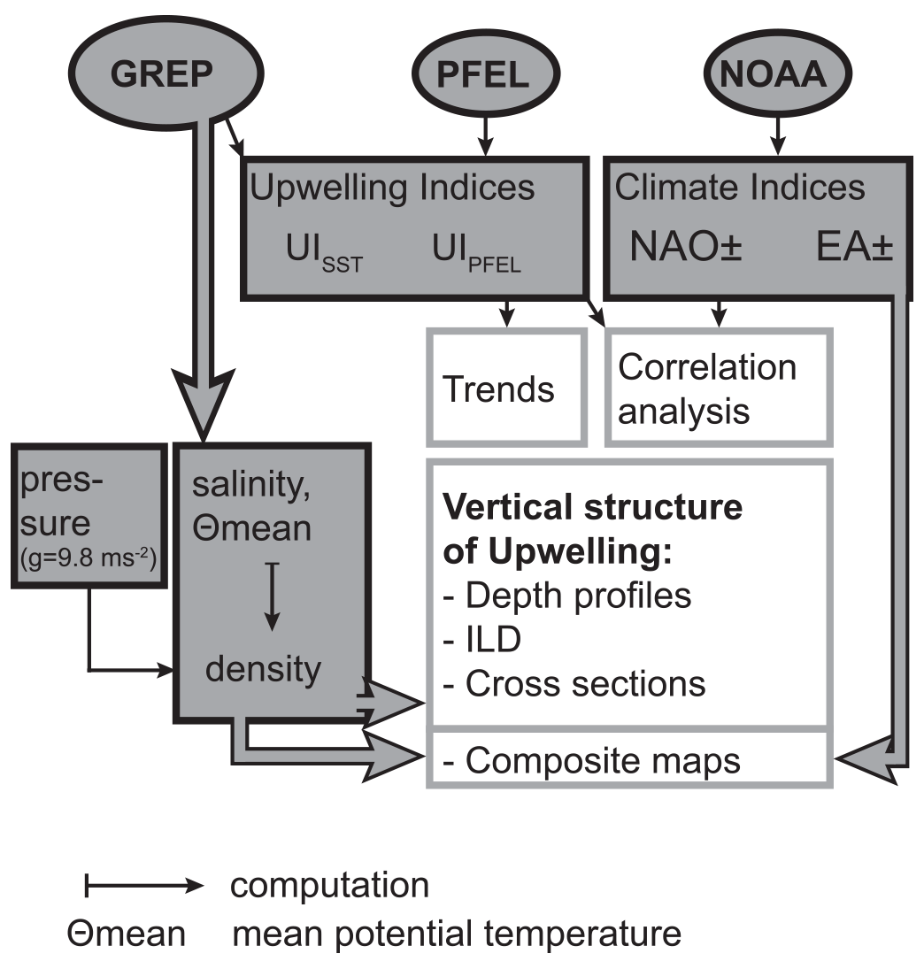
Figure 1 Flow chart of the data sources for the vertical structure of the ocean (GREP: Global Reanalysis Ensemble Product data by Copernicus), the upwelling indices (UI; PFEL: Pacific Fisheries Environmental Laboratory by NOAA), the climate patterns (NOAA: National Oceanic and Atmospheric Administration; NAO: North Atlantic Oscillation; EA: East Atlantic pattern), and the processing sequence (ILD: isothermal depth layer).

The occurrence of upwelling is dependent on the direction and strength of the Ekman transport. The latter is a result of the prevailing wind conditions and the local bathymetry, as well as the coastline geometry and the Coriolis force (i.e. Cropper et al., 2014; Gómez-Gesteira et al., 2008). Upwelling is determined using two different approaches: upwelling based on the sea surface temperature (UI_SST) and based on wind data (UI_PFEL).

The UI_SST is computed using the mean temperature at the shallowest depth (0.50576 m) available in the GREP dataset and is equal to the thermal difference between the offshore (SST_offshore) and coastal (SST_coast) areas at a given latitude and time (Eq. 1):

$$\begin{array}{}\text{(1)}& {\text{UI}}_{\text{SST}}={\text{SST}}_{\text{offshore(lat,time)}}-{\text{SST}}_{\text{coast(lat,time)}}.\end{array}$$

The SST_coast and SST_offshore contain all grid cells in the near- and offshore areas, respectively. A positive UI_SST indicates cooler temperatures near the coast. Upwelling events are recognized when the UI_SST exceeds the 5 ^∘C threshold. This is an upper bound to the thermal upwelling thresholds (varying between 2 and 5 ^∘C) used in other studies of the CCUS (Benazzouz et al., 2014; Cropper et al., 2014; Nykjær and Van Camp, 1994).

The data for the wind-driven upwelling index (UI_PFEL) have been downloaded from the global monthly upwelling index database provided by the Pacific Fisheries Environmental Laboratory (PFEL) from the US National Oceanic and Atmospheric Administration (NOAA; NOAA Fisheries, 2019: https://oceanview.pfeg.noaa.gov/services, last access: 23 July 2020). The dataset provides the results for the zonal and meridional components of the Ekman transport (Bakun, 1990; Bakun and Nelson, 1991) and allows the computation of the upwelling index in consideration of the prevailing coastline geometry using a function for Python which is also provided by NOAA.

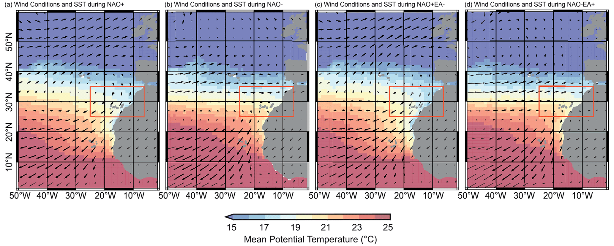
Figure 2 Wind conditions and SST during positive and negative NAO and during combined opposite phases of the NAO and EA. Wind data obtained from ERA5; SST data obtained from Copernicus (for detailed information on NAO+, NAO−, NAO+EA−, and NAO−EA+, see Table 1 and Fig. 4).

The NAO and EA climate indices were retrieved from NOAA's Climate Prediction Center (NOAA, 2020a, b: https://psl.noaa.gov/data/climateindices, last access: 5 July 2020) at a monthly temporal resolution and were aggregated for the winter months, from December to March (DJFM). NOAA calculates these indices by rotated PCA (principal component analysis) of monthly means of the 500 mb geopotential height anomaly over the Northern Hemisphere. Positive and negative phases of the NAO and EA indices are defined by winter index values above 0.5 and below −0.5, respectively (Table 1, Fig. 4; Trigo et al., 2004).

Table 1 Phases of NAO+ and NAO− with the corresponding phases of the EA. Combined opposite phases are marked in bold.

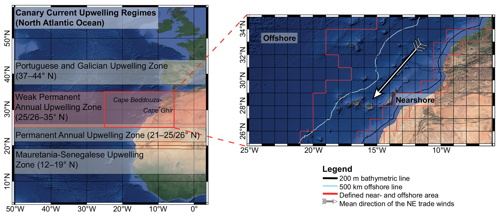
Figure 3 Upwelling regimes in the Canary Current upwelling systems and the nearshore area of the study region (modified after Arístegui et al., 2009; Cropper et al., 2014; © Google Earth 2022).

The vertical structure of the ocean is inferred from variations of the seawater's density and temperature throughout depth. Assuming a constant change of pressure with depth and the use of the gravitational acceleration of the Earth (g=9.8 ms⁻²), the density is computed from the salinity, pressure, and mean temperature (GREP data) using the Gibbs Seawater (GSW) toolbox for the Thermodynamic Equation of Seawater 2012 (TEOS-10; McDougall and Barker, 2011). Subsequently, vertical profiles of density and temperature have been extracted and plotted from the GREP grid at times (months) corresponding to detected upwelling events. The extraction has been carried out separately for the coast and offshore areas for each latitude between 25.5 and 34.5^∘ N at 1^∘ latitude steps.

In the upper ocean, changes in the kinetic energy from radiation, winds, waves, or horizontal advection by currents, among other factors, lead to mixing of the water up to a certain depth. The isothermal layer depth (ILD) corresponds to the maximum depth of ocean mixing and, therefore, to the thickness of the physical properties (temperature) of the ocean being quasi-homogeneous. In this study, the ILD is defined as the depth where the temperature differs by less than 0.8 ^∘C from the temperature at the reference depth of 9.82 m (Chu and Fan, 2010, 2011; Kara et al., 2000). The ILD has been computed for each upwelling event. In addition, to examine the impact of climate patterns on the ocean stratification, the mean ILD has also been computed for positive and negative phases of the NAO, the combined opposite phases of the EA, and for their neutral phases.

The upwelling indices have been correlated with each other and related to the coast and offshore mean ILD. Additionally, these variables (upwelling indices (UIs) and ILD) were correlated with the climate patterns (NAO and EA). The relationships have been tested using the Pearson's correlation coefficient at a significance level of 0.05. The analysis of trends in the time series has been assessed using a linear regression model. Finally, composite maps have been created to explore the links between upwelling indices, the vertical structure of the ocean, and the climate patterns. The composite plots of upwelling are obtained by summing and averaging the temperature of each grid cell for all months with a positive and negative NAO, as well as for months with combined opposite phases of NAO and EA (average computed for the winter months (DJFM) of the years listed in Table 1).

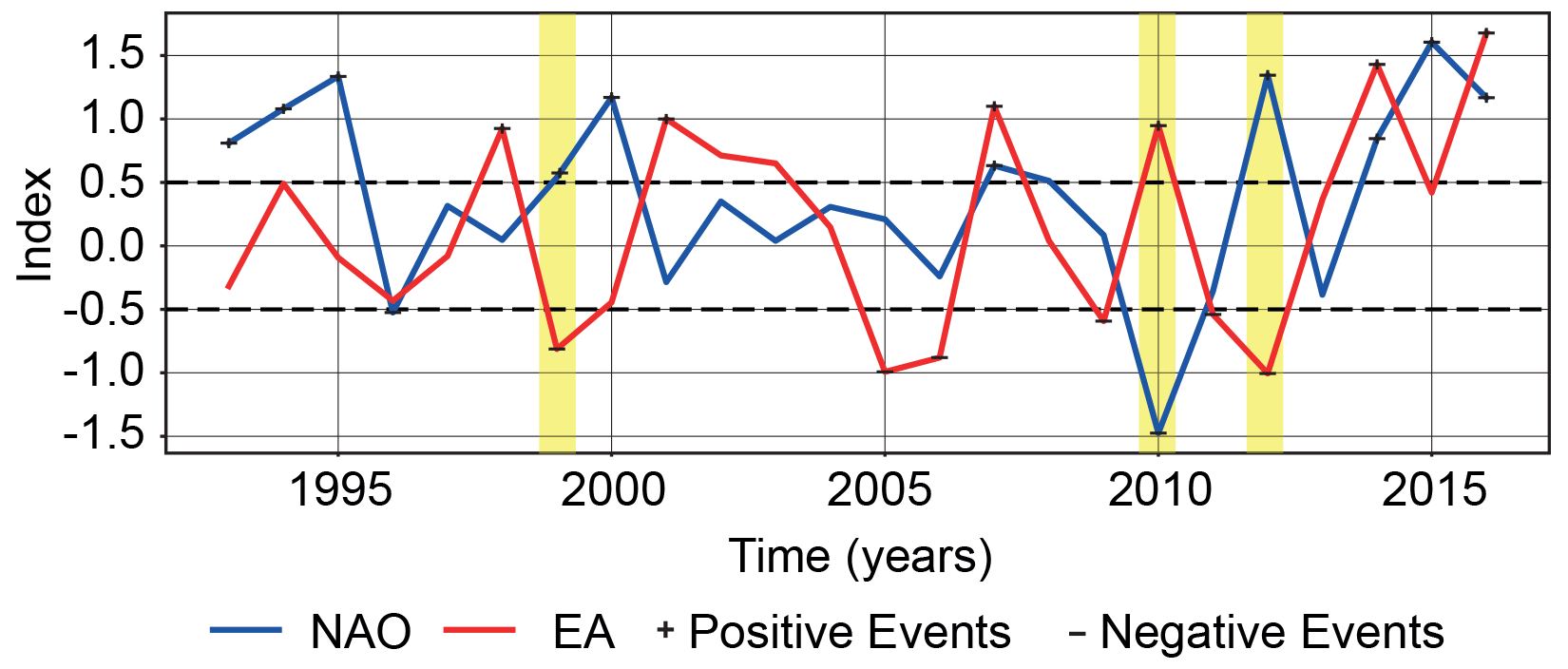
Figure 4 Winter means of NAO and EA. Positive and negative phases are marked with + and −, respectively; combined opposite phases are marked in yellow.

3 Results and discussion

3.1 Upwelling indices and climate patterns: trends and correlations

The normalized upwelling indices have been plotted in a grouped boxplot showing their distribution per latitude (Fig. 5a). All UIs reveal uni-modal distributions, with the UI_SST data being spread widest and UI_PFEL data being slightly negatively skewed. The highest UI_SST occurs around 27.5^∘ N, followed by decreasing values with increasing latitude. The UI_PFEL shows a similar decreasing tendency with increasing latitude. When analysed as a function of time, the time series of the UI_SST and UI_PFEL (1993–2017) reveal mostly positive values and a predominant occurrence of upwelling with a clear annual cycle (Fig. 5b, c). The highest values of the indices corresponding to the exceedance of the upwelling thresholds occur in summer and early autumn, especially in July and September. Besides the variation on the temporal scale, the strength of the upwelling events and their spatial extent differ among indices. Overall, the results of the current study are in accordance with Narayan et al. (2010) and underline the issue of upwelling indices being very dependent on the used datasets and processing methods. The results show the importance of studying upwelling using several methodologies and of adapting the calculation of indices to each geographical location in order to make adequate predictions of their variability in the future.

The impact of the climate patterns on the upwelling indices is well illustrated in Fig. 5, which displays UI_SST (Fig. 5b) and UI_PFEL (Fig. 5c) averaged over years of positive and negative phases (e.g. UI_SST for NAO+ corresponds to monthly values averaged over NAO+ years). Averages over all the years (1993–2017) and averages over years of coupled phases (marked in bold in Table 1) are also shown for comparison. More differentiated and consistent relationships can be inferred for UI_SST than for UI_PFEL, particularly from December to July (Fig. 5c). Larger values of UI_SST are associated with positive phases of the winter NAO, as expected due to the strengthening of the alongshore winds during NAO+ (Fig. 2). However, Fig. 5 also shows that maximum upwelling indices occur in years of NAO+EA− combinations, while minimum values occur during either NAO− years or NAO−EA+ combinations. Additionally, the time lag between the UI_SST and UI_PFEL differs with the phases of the climate pattern. During years of NAO+EA−, the time lag of maximum index values is reduced to 1 month, while during the other phases and throughout the whole period of the study, a greater time lag of 2 months becomes visible, as found in previous studies (Benazzouz et al., 2014; Nykjær and Van Camp, 1994). This time lag has been ascribed to the influence of the bottom topography (Nykjær and Van Camp, 1994), differences in the inertia of atmosphere and ocean, and advection processes (Benazzouz et al., 2014). Additionally, other factors such as wind stress curl, stratification, and onshore geostrophic flow may contribute to the time lag, as they interfere with the upwelling process and condition the upper-ocean response to the wind forcing (Marchesiello and Estrade, 2010).

Due to the limited number of years (only 2) in which coupled NAO+EA− conditions occur (Table 1), caution is required in generalizing this result. Nonetheless, these results are qualitatively similar to a recent analysis of the impact of opposing NAO and EA phases during winter on precipitation, groundwater levels, and wind power generation in Portugal (Neves et al., 2019, 2021).

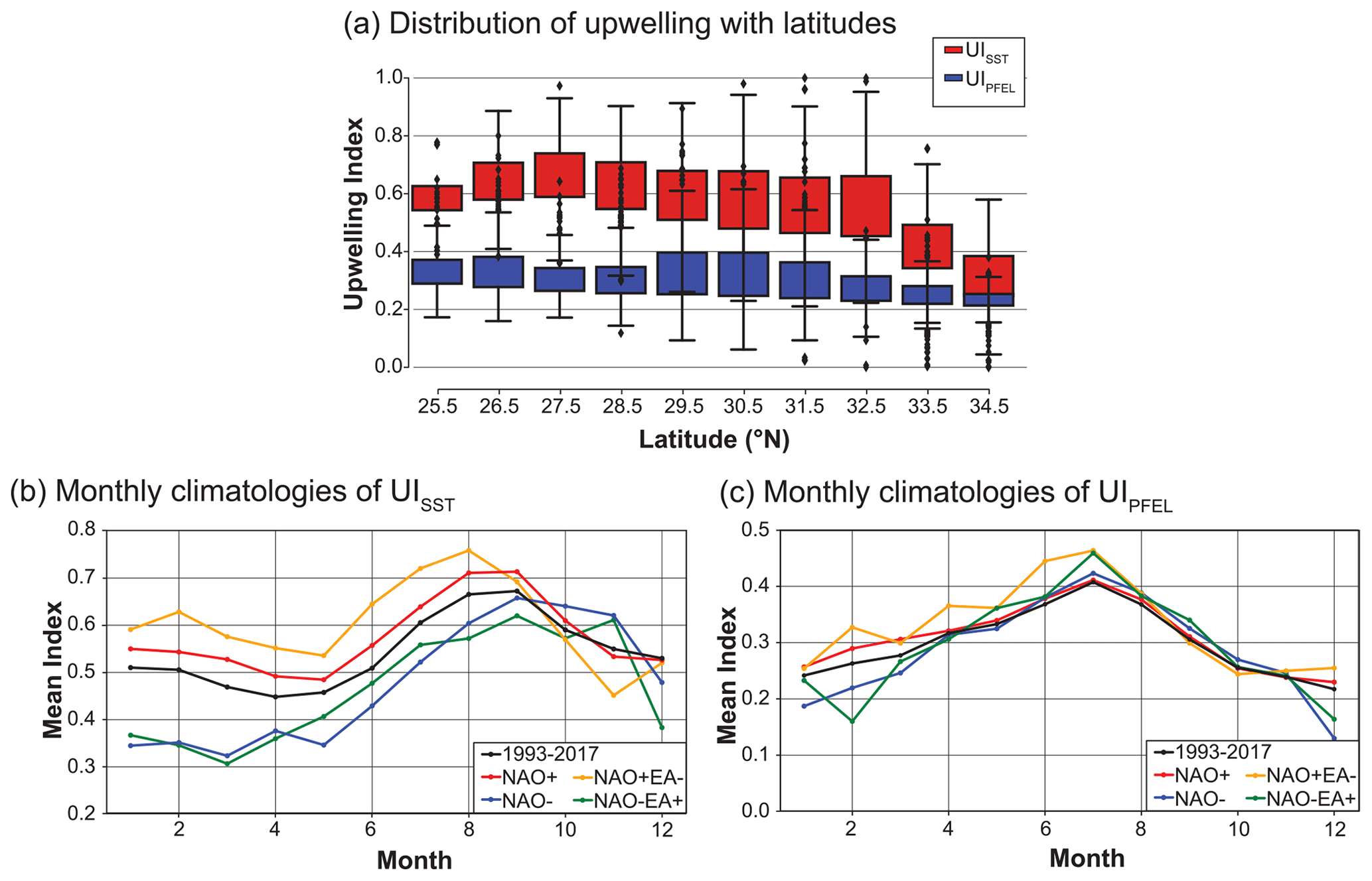
Figure 5 Boxplot of normalized upwelling indices as a function of latitude (a) and monthly climatology of normalized UI_SST (b) and UI_PFEL (c) during different phases of the climate patterns and throughout the study period (1993–2017).

Calculated trends for the whole period of the study are small and show mixed negative (−0.0008, UI_SST) and positive (0.1, UI_PFEL) tendencies in all upwelling indices, with differences depending on the latitudes. Therefore, no consistent trend has been detected in either of the UIs during the selected timeframe of 25 years. These results rather indicate a stable coastal upwelling during the past decades and give no support to previous contradictory findings of either an intensification or weakening of upwelling in the CCUS. Previous studies leading to the controversy (Bakun, 1990; Cropper et al., 2014; McGregor et al., 2007; Narayan et al., 2010; Polonsky and Serebrennikov, 2018) considered time spans of 30–60 years; hence, differing results can also be due to the temporal scale, and the short time period used for this study should be used with caution when an assessment of long-term changes is done (Abrahams et al., 2021). Additionally, the usage of different datasets and defined study areas and thresholds makes a comparison less robust.

The correlations of the UI_SST and the UI_PFEL are all significant, with a moderate correlation between the indices (UI_SST versus UI_PFEL: 0.437). Average winter upwelling indices show moderate to good correlations with climate indices, especially the wind-based upwelling index and NAO. Good correlations between the winter NAO, wind intensity along the CCUS, and upwelling had already been observed in previous studies (Cropper et al., 2014; Marrero-Betancort et al., 2020).

3.2 Vertical structure of upwelling

The vertical structure of the upper ocean during upwelling is the same regardless of the upwelling index used (wind-based or SST-based). The cross-sections in Fig. 6 are examples of composite maps showing the temperature at two particular latitudes. The first corresponds to the sum of 3 upwelling events detected at 26.5^∘ N, while the second corresponds to the sum of 14 events detected at 30.5^∘ N. Higher temperatures at the surface are clearly seen offshore to the west of 30^∘ W, while cooler temperatures near the coast indicate active upwelling. The cold-water plume with temperatures of less than 18 ^∘C ascends from depths of more than 200 m and distances of more than 1500 km from the coast. At the surface, the vertical flow narrows and is focused at less than 100 km from the coastline, but the precision of its detection is limited by the resolution of the dataset. The isotherms are closer to each other at the surface in the offshore area, with an increasing space between them with depth and towards the coast. The cooler temperatures along the continental shelf and the gradient of the isotherms sloping towards the surface clearly indicate the vertical flux of subsurface water towards the surface (Ekman suction) in order to replace the offshore Ekman transport of surface water. With depth, the stratification increases, and the differences between the near- and offshore area decrease. Extracted vertical profiles (not shown) confirm these findings, with surface temperatures of around 20 ^∘C for upwelled waters along the coast and 25 ^∘C for surface water offshore, whereas salinity values are higher at the coast compared to the offshore area. The longitudinal thermal and haline differences decrease with depth and vanish below a depth of 100–150 m.

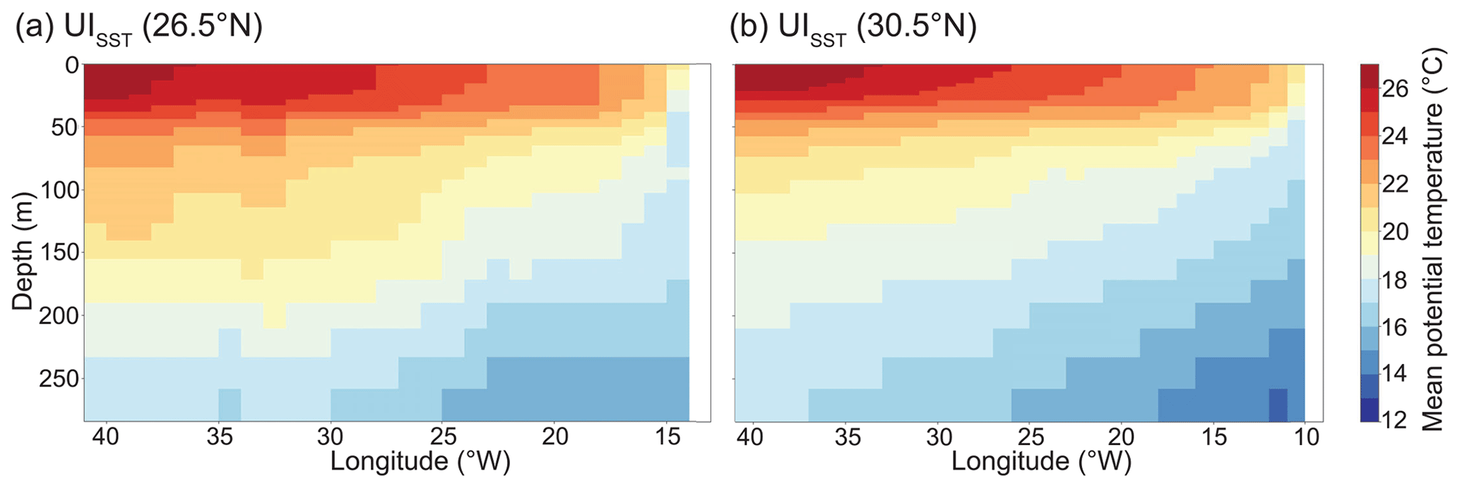
Figure 6 Vertical cross-sections of temperature during upwelling at 26.5^∘ N (a) and 30.5^∘ N (b).

Based on the climatology of the vertical water column velocity, derived from the Global Ocean Data Assimilation System (GODAS) reanalysis, the region around 30^∘ N has been identified as an area where upwelling weakens occasionally (Cropper et al., 2014). However, the cross-section at 30.5^∘ N displays slightly more intense upwelling than the cross-section at 26.5^∘ N (Fig. 6). In fact, these differences in the vertical structure of upwelling at different latitudes are not particularly significant and reveal the spatio-temporal variability of the intensity of upwelling in the study area. That variability is mainly a consequence of changes in the strength and meridional position of the trade winds but is also affected by the width and shape of the continental shelf, as well as by local wind circulations related to the orography and land–ocean contrasts (Bessa et al., 2019, 2020). Despite that variability, the results of this study indicate stable coastal upwelling conditions extending from 26^∘ N up to 32.5^∘ N, which is in agreement with other works (Arístegui et al., 2009; Cropper et al., 2014; Nykjær and Van Camp, 1994).

The ILD represents the limit of the sea–air interaction at these scales and thus the maximum depth until which mixing influenced by kinetic energy in the ocean occurs (Chu and Fan, 2011; Sprintall and Tomczak, 1992). In the study region, the ILD shows a strong annual cycle, with shallower mean depths in summer (∼20 m) than in winter (100–120 m). In general, deeper ILDs during winter are explained by increased storm activity, stronger winds, and greater heat losses at the surface, as well as by negative buoyancy forces leading to more efficient mixing (Troupin et al., 2010; Yamaguchi and Suga, 2019). During summer, in contrast, high stratification is favoured due to greater surface warming through solar radiation (Barton et al., 2013). Still, when compared to normal summers, we observe a deepening (of 1 to 2.5 m) of the ILD during upwelling events, especially nearshore. Nevertheless, the ILD alone is not an sole indicator of upwelling, as alongshore wind and Ekman transport play the major role (Benazzouz et al., 2014; Polonsky and Serebrennikov, 2018).

3.3 Signature of climate patterns on the vertical structure

The impact of the NAO and EA on the vertical structure of the ocean is only visible in winter, since their influence is supplanted by the strengthening of trade winds during summer months. Horizontal composite maps of the temperature are presented for the NAO phases, and for their combination with opposite phases of the EA, at different depths (Fig. 7). Besides considering the temperature at the surface (0.51 m), the depth steps in the upper ocean have been chosen according to the range of the ILD observed in the winter months. The lowest depth displays the conditions where the influence of the atmosphere through wind and heat flux is largely absent.

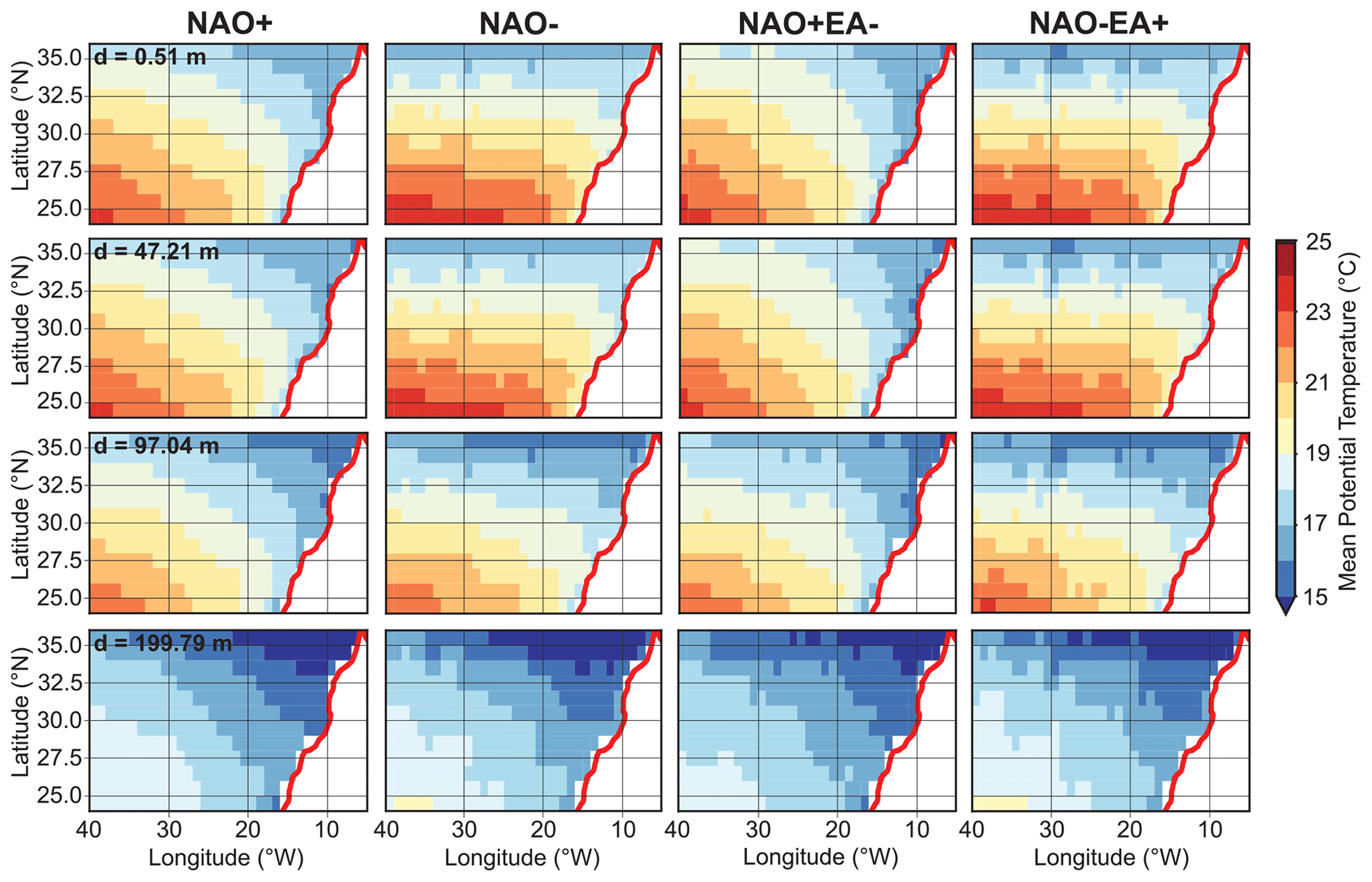
Figure 7 Composite maps of temperature for positive and negative NAO and opposite NAO and EA phases showing the spatial extent of upwelling at different depths; red line represents the coastline. For NAO+, 48 months (12 winter means) where used; for NAO−, 8 months (2 winter means) were used; for NAO+EA−, 8 months (2 winter means) were used; and for NAO−EA+, 4 months (1 winter mean) were used.

There is an overall northeast to southwest gradient in the temperature, with colder waters in the NE and warmer waters in the SW corners of the study region (Fig. 7). In addition, one can observe a narrow strip of cold water (temperature <18 ^∘C) adjacent to the coastline, which is indicative of upwelling. The NE–SW temperature gradient and upwelling zone are more evident during NAO+ and coupled NAO+EA− phases, particularly at the surface and at ∼50 m depth. The temperature gradient persists at deeper levels (∼100 and 200 m), but at these depths, the patterns are nearly identical regardless of the climate phases. In contrast, the superficial patterns (depth ≤50 m) display a more meridional distribution during NAO− and NAO−EA+ phases, particularly in the offshore, with more reduced upwelling near the coastline. The observed patterns in the ocean temperature are a footprint of the large-scale atmospheric patterns during the winter. Thus, during NAO+ phases, the strength of the Azores high-pressure system increases and generates stronger NE winds in the study region, with the opposite occurring for NAO− phases (Fig. 2). The stronger (weaker) winds for NAO+ (NAO−) can explain the intensified (lessened) upwelling and NE–SW temperature gradients at the ocean superficial levels.

Despite the moderate resolution of the dataset, it is also interesting to note that the intensity and extent of the upwelling strip along the coastline is greatest for combined NAO+EA− events. The extreme upwelling signature of these events can be observed down to ∼50 m depth. On the other hand, the persistence of the same temperature patterns at deeper levels (>50 m), regardless of the climate phases, indicates higher inertia to changes and larger memory effects at depth and is consistent with the stable directions (NE–NNE) of the predominant winds in this region, despite the seasonality in their intensity (Marrero-Betancort et al., 2020).

The average ILD during winter months (DJFM) for different phases of the climate indices confirms the importance of the combined influence of the NAO and EA in the generation of extremes (Fig. 8). The ILD is greatly influenced by weather patterns and presents opposite variations at the coast and offshore areas. Variations are at a maximum near the coast (up to ∼40 m) between a minimum of 75 m for NAO+EA− phases and a maximum of 155 m for NAO−EA+ phases. Deepening of the ILD near the coast with NAO+EA− coupled phases is consistent with intensified alongshore NE winds, intensified Ekman transport, greater upwelling, and, therefore, greater vertical mixing. The opposite shallowing of the ILD occurs for NAO−EA+ phases when there is a weakening of NE winds and very little sign of upwelling.

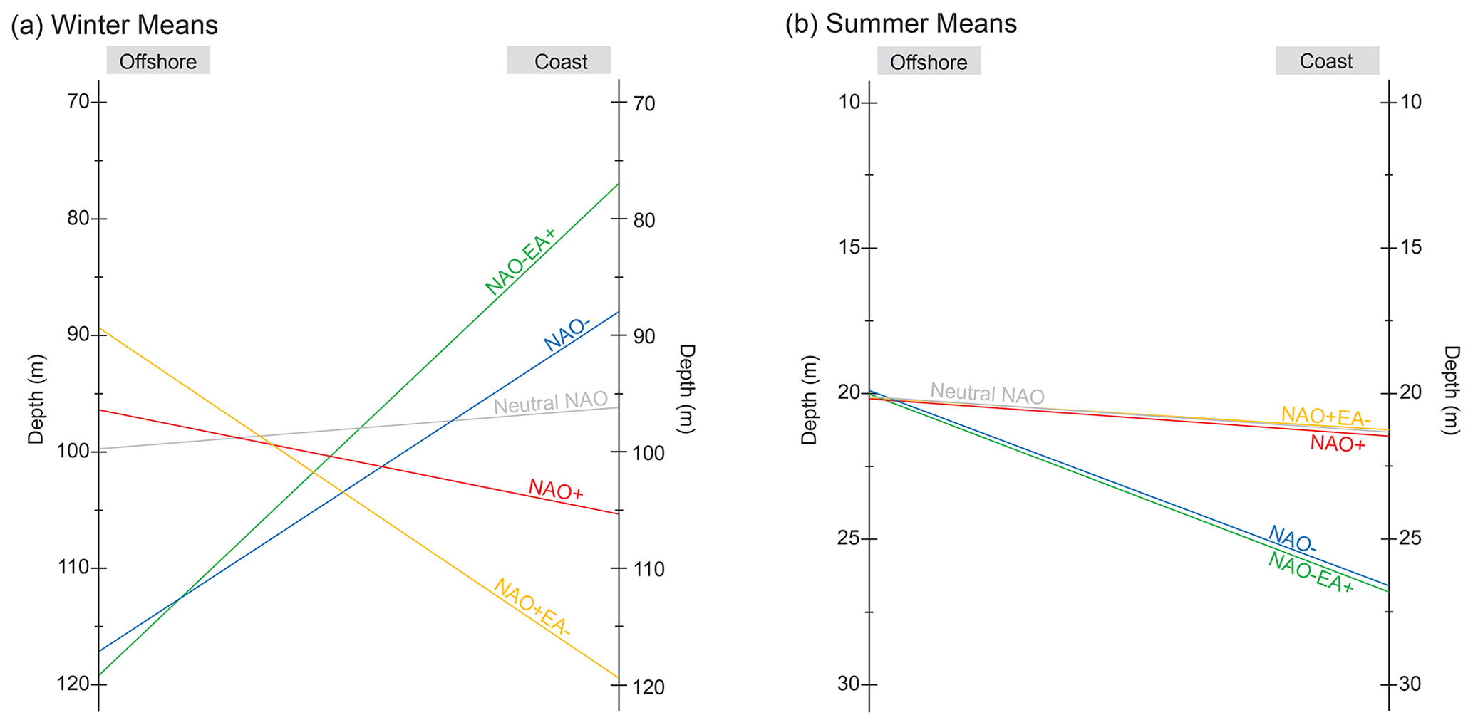
Figure 8 Schematic representation of the mean ILD for NAO and EA phases during winter (a) and summer (b).

The influence of the NAO and EA on winter upwelling along the CCUS had already been recognized by Cropper et al. (2014), among others (e.g. Benazzouz et al., 2014; Bonino et al., 2019; McGregor et al., 2007; Narayan et al., 2010). However, few studies so far have recognized the importance of interactions among the NAO and EA, and only recently did we become aware that their couplings or superpositions, as well as the temporal shifts in their synchronization, may prompt extremes in several land variables such as net biome productivity, global land carbon sink, or aquifer levels (Bastos et al., 2016; Cleverly et al., 2016; Neves et al., 2019). The present study further extends previous results on the role of the NAO and EA in the study area by showing that coupled NAO+EA− phases also correspond to extremes in upwelling along the CCUS during winter.

4 Conclusions

The temporal and spatial extent of upwelling along the Canary Current upwelling system was analysed from 1993–2017 using modelled data with in situ validations from GREP. Even though the used dataset might not reflect the in situ conditions to their full extent, the results of this study contribute to a better understanding of the ocean structure and upwelling. In this study, two different upwelling indices have been calculated: one based on the SST data (UI_SST) and one based on wind data (UI_PFEL). The results of the indices differ in their strength and extent, but both reveal upwelling in the selected area between 25 and 35^∘ N. Small negative or positive trends of the calculated indices imply stable coastal upwelling conditions over the past 25 years.

During detected upwelling events, the surface waters are cooler and denser at the coast in comparison to the offshore values, resembling Ekman transport towards the offshore area and Ekman suction along the coast. This signature is represented by the isotherms sloping towards the surface in the coastal area, as shown in the cross-sections of the temperatures for upwelling events. The differences in temperature between the near- and offshore area decrease with depth. Ocean mixing and stratification were assessed through the calculation of the ILD. Dependent on the increased storm activity during the winter months and, therefore, an increased air–sea interaction, the ILD deepens in winter and lowers in summer. An additional deepening of the coastal ILD was observed during upwelling events.

The changes of the ILD are striking when taking the climate patterns into account. The strengthening of the Azores high-pressure system during winter with NAO+ and the resulting stronger NE trade winds lead to enhanced mixing of the upper ocean in the coastal area. Thus, the ILD deepens along the coast and gets shallower in the offshore area. The opposite can be observed during NAO− years, and both occurrences are intensified during years of coupled, opposite phases of NAO and EA. The same impact of synchronized NAO and EA indices becomes visible in the horizontal composite maps (Fig. 7). In years of NAO+, there is a superficial (up to 50 m) temperature gradient from NE–SW and an evident upwelling zone. The latter extends deeper (up to 100 m depth) during NAO+EA− years. In contrast, during NAO− and NAO−EA+, a more meridional distribution can be observed at the surface and offshore, although the NE–SW temperature gradient in deeper levels is persistent regardless of the climate phases. The study suggests that stronger upwelling along the CCUS is observed during coupled NAO+EA− phases, represented by maximum values of both upwelling indices and a deepening of the coastal ILD. It therefore emphasizes the impact of coupled phases of climate pattern on extreme events in the ocean.