Refined estimates of water transport through the Åland Sea in the Baltic Sea

Water exchange through the Åland Sea (in the Baltic Sea) greatly affects the environmental conditions in the neighbouring Gulf of Bothnia. Recently observed changes in the eutrophication status of the Gulf of Bothnia may be connected to changing nutrient fluxes through the Åland Sea. Pathways and variability of sub-halocline northward-bound flows towards the Bothnian Sea are important for these studies. While the general nature of the water exchange is known, that knowledge is based on only a few studies that are somewhat limited in detail. Notably, no high-resolution modelling studies of water exchange in the Åland Sea area have been published. In this study, we present a configuration of the NEMO 3D hydrodynamic model for the Åland Sea–Archipelago Sea area at around 500 m horizontal resolution. We then use it to study the water exchange in the Åland Sea and volume transports through the area. We first ran the model for the years 2013–2017 and validated the results, with a focus on the simulated current fields. We found that the model reproduced current direction distributions and layered structure of currents in the water column with reasonably good accuracy. Next, we used the model to calculate volume transports across several transects in the Åland Sea. These calculations provided new details about water transport in the area. Time series of monthly mean volume transports showed consistent northward transport in the deep layer. In the surface layer there was more variability: while net transport was towards the south, in several years some months in late summer or early autumn showed net transport to the north. Furthermore, based on our model calculations, it seems that dynamics in the Lågskär Deep are more complex than has been previously understood. While Lågskär Deep is the primary route of deep-water exchange, a significant volume of deep water still enters the Åland Sea through the depression west of the Lågskär Deep. Better spatial and temporal coverage of current measurements is needed to further refine the understanding of water exchange in the area. Future studies of transport and nutrient dynamics will eventually enable a deeper understanding of eutrophication changes in the Gulf of Bothnia.

1 Introduction

The Gulf of Bothnia, in the northern Baltic Sea, has so far been in relatively good environmental health and free from both seasonal and long-term hypoxia occurring in many other Baltic Sea basins. Recently evaluated long-term trends, however, show changes in the eutrophication status (Kuosa et al., 2017), including nutrient and oxygen concentrations. Reasons for these changes are currently not fully understood. One piece of the puzzle is the still poorly understood fluxes of nutrient-rich and possibly hypoxic water from the Baltic proper in the south (Ahlgren et al., 2017). The first crucial step on the way to understanding these fluxes is studying the routes of water to and from this area.

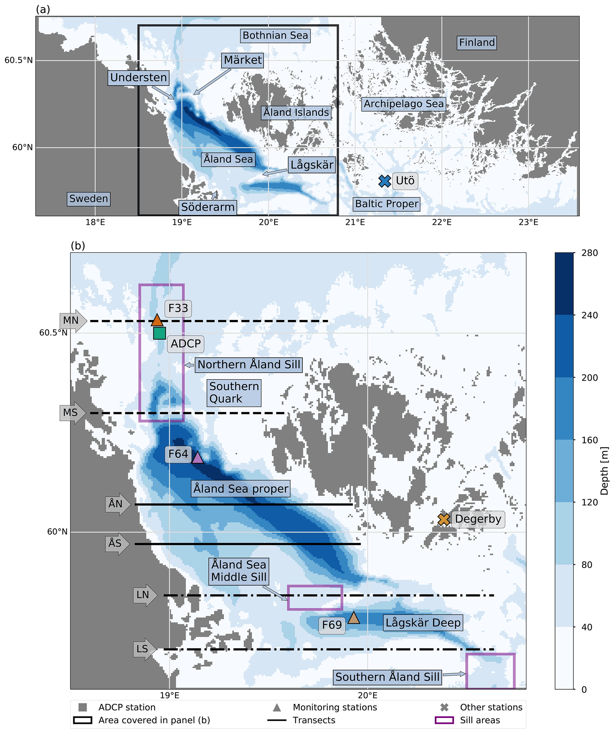
Figure 1 (a) Model domain and bathymetry. The main focus area of this study is shown with a rectangle. In addition, several geographic references are displayed. (b) A more detailed map of the main focus area. Sub-basins and sill areas relevant for the analysis are shown. Furthermore, the locations of stations and transects mentioned in the text are indicated.

Water has two main routes between the Baltic proper and the Gulf of Bothnia: the deeper but narrower Åland Sea and the wider but shallower Archipelago Sea (Fig. 1). A series of sills and smaller sub-basins regulate the exchange in the Åland Sea route, and numerous islands and narrow passages control the exchange in the Archipelago Sea route. Depths in the area vary from just a few metres in the shallow archipelago area to 300 m in the Åland Sea, with many relatively steep topographic gradients along the bottom (Leppäranta and Myrberg, 2009). The mean depth of the Archipelago Sea is only 19 m. It is characterized by numerous small islands and narrow straits.

The Åland Sea has two basins. The smaller Lågskär Deep (also known as the Lågskär Basin or southern Åland Sea basin) has a maximum depth of 220 m, and the larger Åland Sea proper (or the northern Åland Sea basin) has a maximum depth of 301 m. Three sills affect water exchange through the Åland Sea. The southernmost of these is the Southern Åland Sill, which is a narrow channel on the southern edge of the Åland Sea. It is a major barrier for deep water entering from the Baltic proper. Next is the Åland Sea Middle Sill between Söderarm and Lågskär, separating the Lågskär Deep from the Åland Sea proper. The third is the Northern Åland Sill in the Southern Quark area located at the northern edge of the Åland Sea.

Complex bathymetric features, significant depth variations and patchy observational data pose challenges for studying the exchanges between the Baltic proper and the Gulf of Bothnia. Likewise, previous modelling efforts have been hindered by insufficient local resolution and unresolved bathymetric features. In this paper, we present a new high-resolution three-dimensional hydrodynamic modelling configuration for the Åland Sea and the Archipelago Sea. This configuration provides a platform for studying this region. We focus on the Åland Sea to investigate the exchange fluxes through the area.

The first comprehensive study of water exchange between the Baltic proper and the Gulf of Bothnia was probably that of Witting (1908). In the early 1920s, Åland Sea studies were continued through Finnish–Swedish co-operation, with both hydrographic and current meter observations taken in 1922 and 1923. Several hydrographic surveys were conducted in the Åland Sea in the 20th century (e.g. Lisitzin, 1951). In the late 1950s Hela (1958) estimated the water exchange between the Gulf of Bothnia and the Baltic proper using hydrographic data from the area measured in 1956. As was already described by Granqvist (1938) for example, Hela (1958) found that there were no clearly defined water masses and that continuous mixing occurs between waters of different origins. Hela (1958) nevertheless presented TS diagram analysis (calling it in this case “schematic and more or less arbitrary”), which he used to identify a deep-water type originating from water entering from the Baltic proper. The term “deep water” was used to emphasize that this water was not Baltic proper bottom water, as the most saline bottom water is not able to flow over the Southern Åland Sill. Also notable were the warm water lenses below the thermocline and above the temperature minimum, which Hela (1958) analysed to be warm-water intrusions from the Baltic proper. This analysis was later further elaborated by Hela (1973).

Palosuo (1964) evaluated the water exchange using bathymetric information to study the channels and sill depths on the deeper paths leading from the Baltic proper to the Gulf of Bothnia through Lågskär Deep and the Åland Sea. He also concluded from data from station F69 that at Lågskär Deep there is large variability in the salinity in the surface layer up to 80–90 m depth, below which salinity increases constantly to values up to 8 g kg⁻¹. The Åland Sea proper showed similar salinity variation at the surface layer and more constant values in the deeper layers, being less saline than in the Lågskär Deep. A constant northward current was estimated to be present in the deeper layer of the Åland Sea proper based on the datasets in both Palosuo (1964) and Hela (1958).

After these studies, the most recent in-depth investigations concentrating on the water exchange in the Åland Sea were produced within the framework of the Finnish–Swedish co-operation to investigate the environmental condition of the Gulf of Bothnia in the 1970s (Ehlin and Ambjörn, 1977; Ambjörn and Gidhagen, 1979).

These earlier studies relied heavily on observational and mostly short-term datasets. More recently, numerical modelling has made it possible to study currents and water exchanges fully in four dimensions, giving us spatial and temporal coverage not possible with just observations. This allows us to investigate intra- and inter-annual variability, for example, with much richer detail than we could with observations alone.

Modelling studies investigating transports in this area have so far been rare. A notable exception is a study by Myrberg and Andrejev (2006). Although they concentrated mainly on the Gulf of Bothnia as a whole, they also looked at water exchange in the Åland Sea–Archipelago Sea area. They found that transport estimates had significant uncertainty and depended on the choice of averaging timescales for velocities and transports and on the chosen locations of the cross sections used for inflow and outflow estimates.

The main aim of this paper is to investigate modelled routes of water through the target area with a high-resolution model configuration. We also study their variability on a monthly scale and evaluate the reliability of the estimates. This information will provide the basis for future studies of transport dynamics in the area and serve as the first step for future investigations, which will enable us to understand why and how the eutrophication status in the Gulf of Bothnia is changing.

Our modelling configuration is based on the NEMO model core (Madec and NEMO System Team, 2019), which has previously been applied at high resolution in the nearby Gulf of Finland (Vankevich et al., 2016; Westerlund et al., 2018, 2019). The Archipelago Sea has been previously modelled at high resolution by Tuomi et al. (2018) and Miettunen et al. (2020), who used the COHERENS model (Luyten, 2013). The configuration presented in this study builds on that experience, but also covers the Åland Sea, which was not included in the COHERENS setup. In their study Tuomi et al. (2018) found that the σ coordinates used in the COHERENS implementation introduced over-mixing, especially in deep channels where there were large depth gradients from one grid point to the next. To mitigate this issue, we chose the z^∗ vertical coordinate system for our implementation. This is a geopotential vertical coordinate system where sea surface height variations are distributed over the whole water column (e.g. Klingbeil et al., 2018). It has been successfully applied in the aforementioned Gulf of Finland configuration, as well as in regional configurations (Hordoir et al., 2019).

Bathymetric features greatly affect water exchange in this topographically complex and irregular area. Forming a correct understanding requires detailed information about exchange pathways and sill depths, for example. In principle, bathymetric data are available from different sources with high spatial resolution; see, e.g. the Baltic Sea Bathymetry Database (BSBD), available at http://data.bshc.pro (last access: 4 January 2022), or the European Marine Observation and Data Network (EMODnet) bathymetry, available at https://www.emodnet-bathymetry.eu (last access: 4 January 2022). However, the resolution and accuracy of the source data are not equally good in all areas; see, e.g. Jakobsson et al. (2019) for an example from the Åland Sea. For this paper, we took a significant effort to ensure that bathymetric features in key areas are represented as realistically as possible in the model.

In this paper, we first introduce the new modelling configuration. Following this, as this is the first time such a high-resolution model has been applied to the Åland Sea, a validation of a 5-year model run is carried out. After that, we investigate modelled currents and finally study volume transports through the study area. These results are then compared to earlier estimates, and future directions for research are charted.

2 Materials and methods

2.1 Modelling methods

We set up the NEMO three-dimensional hydrodynamic model version 4.0.3 for the Åland Sea and the Archipelago Sea at 0.25 nmi (nautical mile) or approximately 500 m horizontal resolution. Model domain and bathymetry are depicted in Fig. 1. The modelled time span covered June 2012 to December 2017, but in our analysis we concentrate on results starting from January 2013 to ensure that the model had a long enough initialization period.

The model setup used the z^∗ vertical coordinate system. There were 200 vertical levels. Level thickness increased slightly with depth, being 1 m at the surface and 1.1 m at 120 m depth. Below the depth of 120 m, the thickness increased more rapidly to about 8 m at the very bottom. This arrangement allowed for the top part of the water column to be resolved at a relatively high resolution while keeping the number of levels manageable.

Horizontal viscosity was parameterized with the Smagorinsky formulation (Smagorinsky, 1963). Smagorinsky formulation has been a popular choice for studying nearby sea areas; see, e.g. Zhurbas et al. (2008). In the vertical, we used the GLS (generic length scale) mixing scheme configured to produce the k-ϵ model. This parameterization has previously been successfully applied in Baltic Sea NEMO configurations (e.g. Hordoir et al., 2019; Westerlund, 2018), and it has been able to reproduce seasonal stratification in the Bothnian Sea quite well (Westerlund and Tuomi, 2016).

We used a sea ice model with a thermodynamic formulation (as was previously done for the Gulf of Finland by Westerlund et al., 2018, 2019). This somewhat eased the relatively high computational requirements of this configuration. During our study period, the ice seasons in the Baltic Sea area were mostly mild or very mild. In the Åland Sea, within our modelling period there was a notable amount of ice only during winter 2012–2013, which has been classified as an average ice season by the FMI (Finnish Meteorological Institute). The winter of 2017/2018 was also an average ice season, but the ice in the area formed only after our modelling period.

We saved 6 h averages of 3D temperature, salinity and current fields. Sea surface height was recorded at 1 h intervals, while volume transports were saved once a day. We computed volume transports from the model for a number of transects. These were integrated over the whole transect to calculate a time series: $F_{\mathrm{v}}=\iint v\mathrm{d}A=\iint v\mathrm{d}z\mathrm{d}l$. Here v is the velocity across the transect, A is the area of the transect, z is the depth along the transect and l is the length of the transect. We also calculated volume transports per unit length (∫v dz) along the transects to investigate the pathways of water more closely.

2.2 Bathymetric data

We compiled the model bathymetry from two sources. The primary source for bathymetric data was the VELMU (Finnish Inventory Program for the Marine Environment) bathymetry model (Finnish Environment Institute), which covers the Finnish Exclusive Economic Zone (EEZ). For the part of the model domain that is outside the Finnish EEZ, we used the BSBD from the Baltic Sea Hydrographic Commission, which covers the whole modelling domain. The resolution of the VELMU bathymetry model is approximately 20 m, but the resolution of its source data is not as high in all locations. The same applies to any other gridded bathymetry dataset. The bathymetry data for the 0.25 nmi model grid was compiled by calculating the mean of VELMU depth points in each model grid point. BSBD data has a resolution of 0.25 nmi in the Åland Sea.

The bathymetric source datasets have mostly been created and interpolated automatically. In addition, the model grid was compiled from those datasets automatically, resulting in a somewhat patchy grid. For example, the channels crossing the area were not all continuous or deep enough, the sills were typically too shallow, and there were some very steep depth gradients challenging for the hydrodynamic model. To mitigate these issues, we checked and edited the model grid manually to ensure that it represented topographic features in the area as accurately as possible in the 0.25 nmi resolution.

The most crucial places to be modified were the sills and channels that control the water exchange through the Åland Sea. Each sill area (locations indicated with magenta in Fig. 1) and its surroundings were checked manually and edited to equal the known sill depths. The channels in the southern and northern parts of the Åland Sea were also edited to be continuous at a certain depth and overall wide enough (at least 3–4 grid points) so that they would enable appropriate water flow between the basins.

Finally, the modified model depth grid was filtered with a Gaussian filter with a standard deviation of 1.2 grid points to smooth out the steepest bathymetry gradients and ensure numerical stability.

2.3 Forcing and boundary conditions

We subset the meteorological forcing from the ERA5 atmospheric reanalysis provided by Copernicus Climate Change Service (Hersbach et al., 2018). We used hourly 10 m winds, 2 m air temperature, 2 m dew point temperature, mean sea level pressure, precipitation, snowfall rate, shortwave radiation flux and longwave radiation flux fields from the reanalysis to force the model.

The model configuration had open boundaries to the Bothnian Sea in the north and the Baltic proper and the Gulf of Finland in the south. We took lateral boundary conditions and initial conditions for the model from a regional reanalysis configuration (Baltic Sea Physical Reanalysis Product BALTICSEA_REANALYSIS_PHY_003_011) provided by the Copernicus Marine Environment Monitoring Service (CMEMS). Initial conditions consisted of interpolated salinity and temperature fields. Boundary conditions included Flather radiation conditions for sea surface heights at one hour intervals and barotropic velocities at 24 h intervals. FRS (flow relaxation scheme) boundary conditions were applied for temperature and salinity at 1 d intervals. A no-flux condition was applied for the small open-sea segment at the south-east edge of the model domain, which improved the stability of the configuration. This area is quite shallow and far away from the area of interest in this study, and thus a no-flux condition was deemed sufficient for this purpose.

There are eight rivers inside the model domain, all of which are on the Finnish coast. We took daily values of river discharge from the watershed model VEMALA which is an operational, national-scale nutrient loading model for Finnish watersheds (Huttunen et al., 2016).

2.4 Observational data

We used sea surface height from the Föglö Degerby station (see Fig. 1). There are also two other tide gauges within the model domain in Turku and Forsmark. However, we did not use data from these sites as they are not representative of the overall sea level variation in the study area but instead reflect local effects. The Turku tide gauge is located in the inner archipelago on the Finnish coast, and the Forsmark tide gauge on the Swedish coast is set up in a constructed area to monitor water levels for a nuclear power plant.

We also investigated temperature and salinity profiles from three stations in the Åland Sea: F33, F64 and F69 (see Fig. 1). These sites are sampled more often, and their temporal coverage is better than in other stations in the area. However, the number of profiles is still quite modest, and we supplemented them with data from the Utö intensive monitoring station at the southern edge of the Archipelago Sea.

We used current measurement data from a location near the station F33 to study how the model is able to reproduce observed currents (station “ADCP” in Fig. 1). The measurements were carried out with a bottom-mounted 300 kHz Workhorse Sentinel acoustic Doppler current profiler (ADCP). The location was 126 m deep, and the corresponding model grid point was 110 m deep. The measurements ranged vertically from 8 m depth down to 112 m depth at 2 m intervals. This dataset covers the period of 6 August 2016–3 July 2018 with a time interval of 30 min.

The modelled current components were saved as means of 6 h. For the comparison between the measured and modelled currents, we first calculated the 6 h means of the measured horizontal current components and then from these means, calculated the current magnitude and direction. The ADCP data has been quality checked, leaving gaps in the dataset. These gaps due to bad or missing data occurred mainly in the upper 40 m layer during spring and summer. On average, 33 % of the ADCP measurements were missing in the upper layer, but some months lacked up to 77 % of measurements. If a 6 h time slot over which the means were calculated was missing more than 50 % of the measurements, we discarded the time slot both from the averaged ADCP data and from the model data when calculating the bias and current roses.

3 Results

3.1 Model validation

3.1.1 Sea surface height

Adequate accuracy of major sea surface height (SSH) variations is an indication that the model is able to reproduce barotropic dynamics reliably. While the model configuration in this study has not been built for sea level forecasting, a comparison of modelled sea surface height with tide gauge data gives a quick overview of overall model performance. The range of sea level variability and the timing of events are both important when considering the suitability of the model for the study at hand. However, it is good to bear in mind that these results are heavily dominated by how well SSH is presented in the boundary conditions. Furthermore, as the vertical reference for sea level differs between model and tide gauge data, comparison of bias is not feasible.

Figure 2 Sea surface height at the Föglö Degerby tide gauge in 2017, showing a comparison between measurements and the model.

The results from the Föglö Degerby station (see Fig. 1) showed that the model was able to reproduce sea level variations quite well. A part of the SSH time series is displayed in Fig. 2 showing typical results. Most importantly, it shows that the timing of sea level events is quite accurate. There are a few cases where the magnitude of the event was incorrectly estimated in the model, although in most cases the differences were quite small. It is also significant that the range of water level variability is well represented overall. For this station in 2017, the correlation coefficient for the modelled and observed time series was 0.85, and the standard deviation of the observed and modelled values differed less than 3 cm.

3.1.2 Temperature and salinity

The vertical structure of the water column is illustrated with observed and modelled temperature and salinity profiles from three monitoring stations (F33, F64 and F69) in Fig. 3, which shows all available profiles from these stations along with overall mean profiles. In addition, we compared profiles individually to model data to get an overview of model performance. For the study at hand, the ability of the model to estimate the vertical position of the halocline and thermocline correctly is of interest. For example, if the halocline was continuously and severely misplaced in the model, that would likely indicate problems for volume transport calculations.

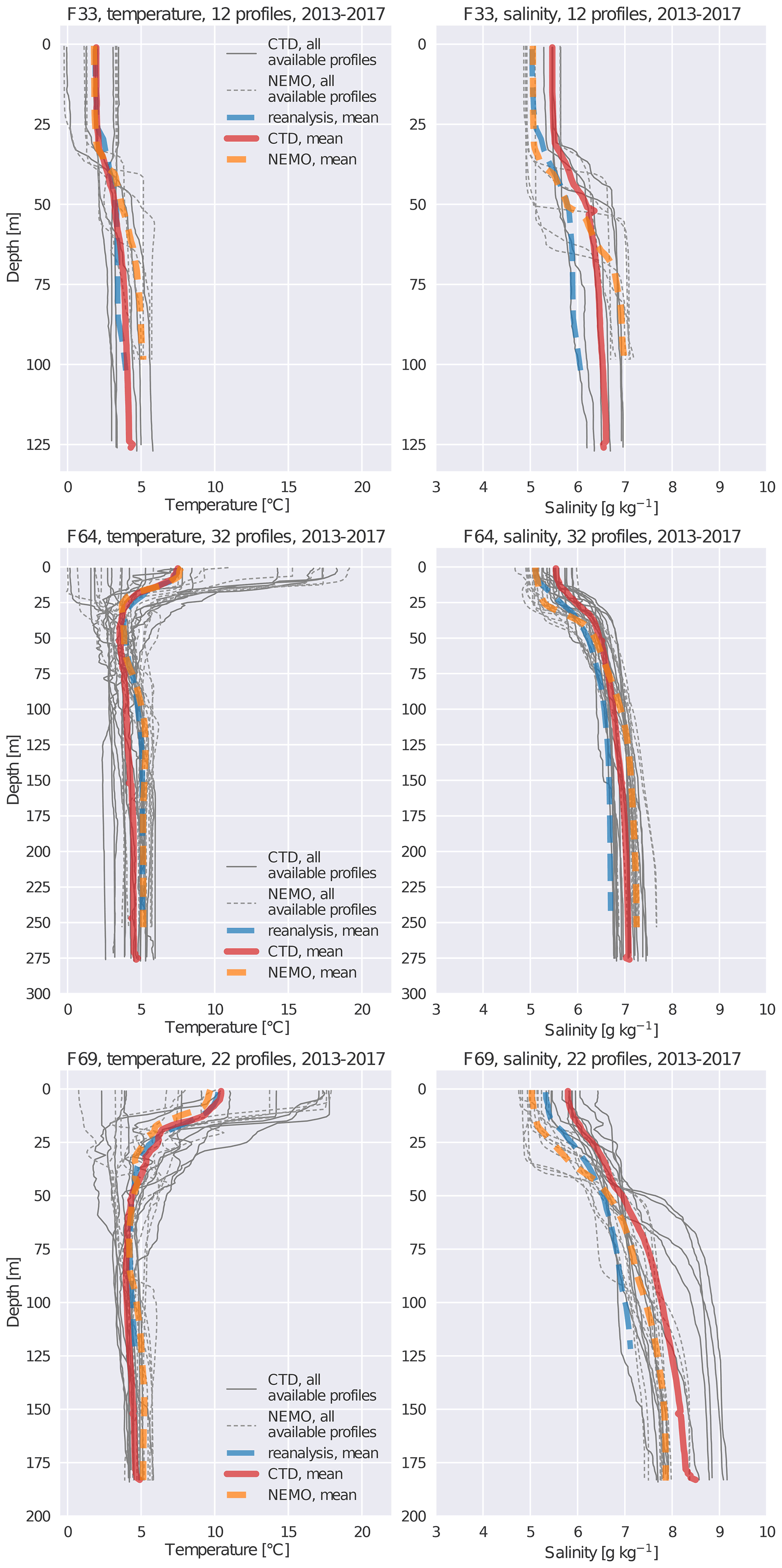
Figure 3 Temperature and salinity profiles from three monitoring stations 2013–2017. All available measurement profiles and corresponding modelled profiles are shown, along with their means. In addition, the mean of the profiles taken from the reanalysis product used as a boundary condition for the model is shown. Please note that the number of profiles varies from station to station.

Vertical temperature profiles were generally quite well reproduced. This includes the strength of the thermal stratification and its vertical position, which were relatively correctly estimated. Salinity profiles revealed that salinity biases are most prevalent near the surface, with typical differences up to 1 g kg⁻¹ above the halocline. Halocline depth in the model was mostly reasonable and the errors in individual profiles were similar to the ones visible in the means. There are some individual profiles, where the model was clearly unable to capture the dynamical situation correctly and where there were errors of 10 or even 20 m in halocline depth. Furthermore, in some cases the shape of the profiles suggested submesoscale activity, which is very difficult to fully model due to the chaotic nature of such phenomena. Overall, the moderate availability of profile data from the modelling area somewhat limits the conclusions that can be drawn based on this data. For instance, almost all profile data available from these stations have been measured in January, May or August. All in all, the ability of the model to reproduce vertical temperature and salinity structure seems to be well within expected accuracy for a state-of-the-art model and the area of interest.

In addition to this, we inspected temperature and salinity time series from the Utö intensive monitoring station at the southern edge of the Archipelago Sea (not shown). Overall, these results indicated very similar model skill to what has previously been reported for the NEMO model in nearby sea areas (see, e.g. Westerlund and Tuomi, 2016; Westerlund et al., 2018). Temperature evolution was quite well reproduced at all depths and seasons, although there were larger differences deeper in the water column. While the frequency of the observations did not allow for a detailed analysis of short-term variability, it does seem that at least some shorter-term events are also reproduced by the model. Salinity observations did not show the same kind of short-term variability as the modelled time series. The general level of modelled salinity values was quite reasonable.

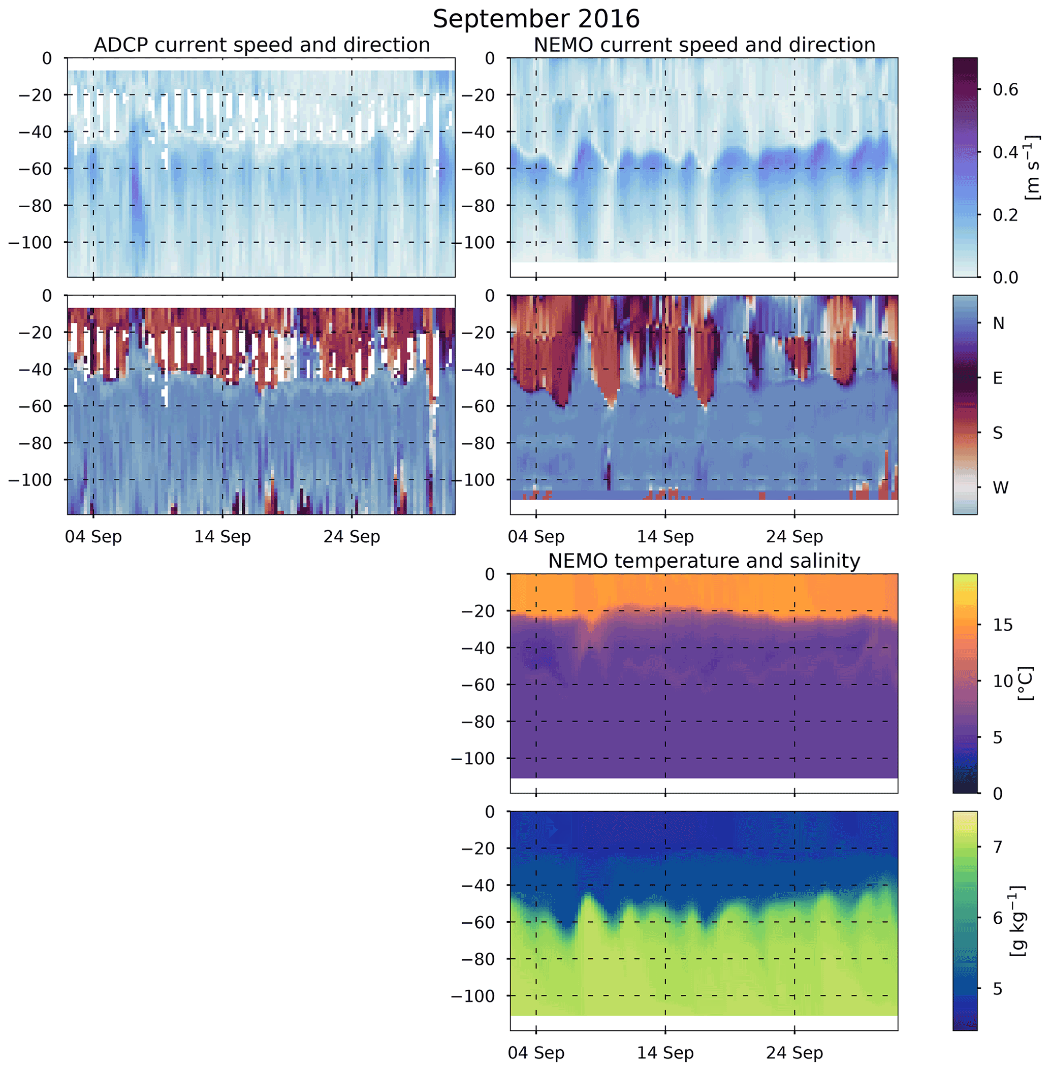
Figure 4 Current magnitudes and directions in September 2016 as measured at the ADCP station and as seen by the model. Modelled temperature and salinity profiles are also displayed.

3.2 Analysis of currents

3.2.1 Simulated and measured currents in the Southern Quark

To evaluate the quality of modelled currents, we compared modelled current magnitudes and directions with observations at the ADCP installation (location shown in Fig. 1). Both model and ADCP data were available for the period of August 2016–December 2017. While time- and space-averaged currents saved from the model often represent different things than the very local observations from ADCP instruments, they can still be used to get an overview of model performance in the area where the ADCP was located.

The vertical profiles of modelled currents had a similar structure as the measured currents. During autumn and winter, there were two layers: an upper layer above the permanent halocline and a deep layer below the halocline (Fig. 4). During the thermally stratified period, three different layers were visible: a surface layer above the thermocline, an intermediate layer between the thermocline and the halocline, and a deep layer below the halocline. The surface layer was more easily visible in modelled current profiles than in measurements, as the ADCP data was missing the upmost 8 m layer. The depth of the thermocline in the model mainly undulated between 10–25 m and the depth of the halocline between 40–70 m (Fig. 4). ADCP current speed and direction data showed that observed halocline depth was mainly between 40–60 m. As we consider mainly current dynamics and transport analysis, the changes of properties occurring at the halocline are more significant than those at the thermocline, for example those regarding the direction distribution of currents. For this reason, we use “upper” or “surface layer” to signify the layer above the halocline and “lower” or “deep layer” to signify the layer below it. We specifically state each time when the intermediate layer is being considered.

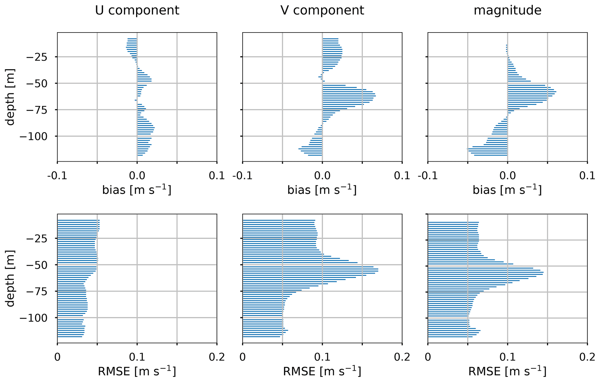
Figure 5 Bias and RMSE in the modelled U (zonal) and V (meridional) current components and current magnitude at the ADCP station from August 2016 to December 2017.

Modelled current magnitudes were highest in the surface layer of a few metres and just below the halocline at depths of 50–70 m. The strongest currents occurred typically in late autumn or winter. In the upper layer above the halocline, the monthly mean current magnitudes varied from 0.09–0.20 m s⁻¹ in the surface to 0.05–0.15 m s⁻¹ at the depths of 10–40 m. At depths of 50–70 m, the monthly means varied from 0.11 to 0.23 m s⁻¹; the highest monthly mean was seen at 60 m depth in February 2017. In the lower parts of the water column, there was less seasonal variation in current magnitudes and the monthly mean current magnitudes decreased with depth from 0.08–0.12 m s⁻¹ at 80 m depth to 0.004–0.013 m s⁻¹ at 110 m depth (representing the deepest model layer at the ADCP station coordinates).

To validate the modelled currents, we calculated bias and root-mean-square error (RMSE) in the modelled horizontal current components and the current magnitude for the period of August 2016–December 2017. In general, the U (zonal) component was underestimated in the upper 30 m and overestimated below that, whereas the V (meridional) component was mainly overestimated above 90 m depth and underestimated below that (Fig. 5). The bias in the current magnitude was small near the surface, increased towards the halocline and decreased again below the halocline. The largest bias and RMSE in the current magnitude occur at depths of the halocline, with values up to 0.061 and 0.145 m s⁻¹, respectively. In the lower parts for the water column, the bias in magnitude was negative, being −0.051 m s⁻¹ at the depth of 112 m, because the model grid point is shallower than the ADCP measurement site.

Both in measured and modelled currents, the dominant current direction was towards the southern sector (SW–SE) in the upper layer and towards the northerly sector (NW–NE) in the lower layer. However, the currents in the upper layer had more variation in direction, and northward-flowing currents also occurred. In the model, these northward currents were vertically more uniform and lasted for longer periods than in the measurements. Moreover, the model showed northward currents at times when the observed current direction was southward. For example, at 10 m depth the measured current directions were mainly towards south and south-east, and the fraction of northward currents (towards sectors NW–NE) was small, 11 % of the whole comparison period August 2016–December 2017 (Fig. 6). The prevailing current direction in the modelled currents was towards the south, but the fraction of northward currents was larger than in the measurements, i.e. 26 % of the whole comparison period.

In the lower layer, there was less variation in the current directions than in the upper layer. For example, at 70 m depth the measured and modelled currents were mainly directed towards north–north-west, but the modelled currents showed a larger fraction of currents over 0.20 m s⁻¹ than the observations (Fig. 6). At 100 m depth, the observed currents were directed towards the north-west and north–north-west, whereas the modelled current direction was dominantly towards the north–north-west. As the current direction at this depth follows the bottom topography, this difference between the observed and modelled current direction is possibly caused by small differences between the real bottom topography and the model bathymetry.

Figure 6 Comparison between measured and modelled currents at the ADCP location. Current roses are shown for 6 August 2016–28 December 2017 at depths of 10, 70 and 100 m. Please note that current roses indicate the direction where the currents flow to.

3.2.2 Seasonality of currents in the Åland Sea

To study the seasonality of circulation patterns both in the surface layer and deeper in the water column, we calculated the mean current field over the period of January 2013–December 2017 (Fig. 7) and the seasonal mean current fields (Fig. 8). In addition, seasonal wind roses from the ERA5 forcing at Märket were inspected (Fig. 9). Winter was defined to be from December of the previous year to February (DJF), spring was from March to May (MAM), summer was from June to August (JJA) and autumn was from September to November (SON).

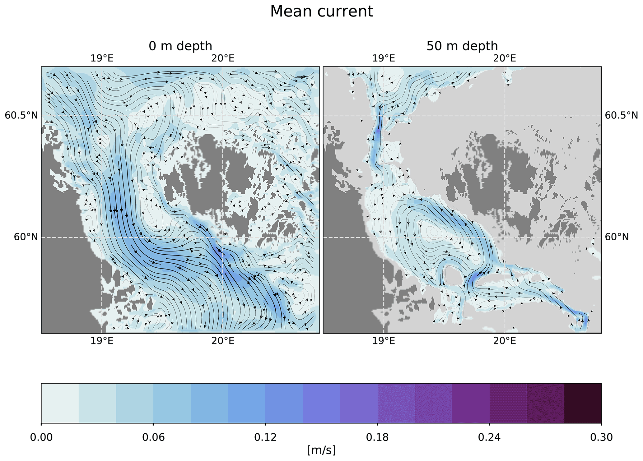
Figure 7 Modelled mean currents at the surface and 50 m depth in 2013–2017.

Figure 8 Seasonal means of modelled surface currents in 2013–2017. Please note that the means of current vectors are calculated as the means of elements in the vector, not as means of magnitudes. This means that in autumn (SON) when current stability is low, magnitudes of mean vectors (shown) are much smaller than means of magnitudes (not shown).

During 2013–2017, the winds at Märket area were most frequent from the W–SSW sector in winter seasons and from SW–SSE and N in spring and summer seasons. In autumn seasons, the most frequent wind direction was from SW, but the directional distribution in the wind rose is otherwise even higher than in the other seasons.

Looking at the surface currents, all the seasonal means showed southward currents through the Åland Sea turning south-eastward or eastward in the southern part of the Åland Sea (Fig. 8). In the eastern side of the Åland Sea, a characteristic feature was a anticlockwise loop existing in autumn, winter and spring. Its location has both seasonal and inter-annual variation. In general, the mean current speeds in the surface layer were stronger at the western side of the basin than at the eastern side.

Autumn was the season with the largest inter-annual variation in current directions, but the southward and south-eastward currents were still dominant in most years. To put it differently, the persistency of surface currents was significantly lower in autumn than in other seasons. This is likely related to the significant inter-annual variability in wind directions during autumn. In summer and spring, there was very little year-to-year directional variation in winds and surface currents. This is visible in the lengths of the vectors in the seasonal mean figure. Although current magnitudes were not significantly smaller in autumn, the mean current vectors are still shorter just because of the component-wise averaging of current vectors.

While most seasons generally had southward currents in the Åland Sea, winter 2013–2014 was somewhat exceptional. During that time, the wind direction at Märket was mainly from the sector between SW and SE, and the surface currents were northward or north-eastward almost in the whole model domain. Winter 2012–2013 showed a large variation in wind directions, the prevailing direction being from NE, while in winters from 2014–2015 onward the prevailing wind direction was from SW or W. The strongest southward currents in winter can be seen in 2016–2017 when the wind distribution was weighed more to westerlies and the portion of southerlies was lower than on average.

Deep-layer currents showed less seasonal variation in direction than surface currents, and the current direction was generally northward in all seasons. Figure 7 shows the mean circulation at 50 m depth as an example. In the southern part of the model domain, the mean current direction was northward and north-westward along the channel that leads to the Lågskär Deep. In the Åland Sea proper, there was a anticlockwise loop covering the whole basin, with stronger currents on the eastern side of the basin. In the northern part of the basin, the currents continued northward along the Southern Quark, and the bathymetry steered the currents north-eastward near the northern edge of the model domain. The persistency of the current direction was high in the narrow channels and also higher on the eastern side than on the western side of the loop in the Åland Sea proper.

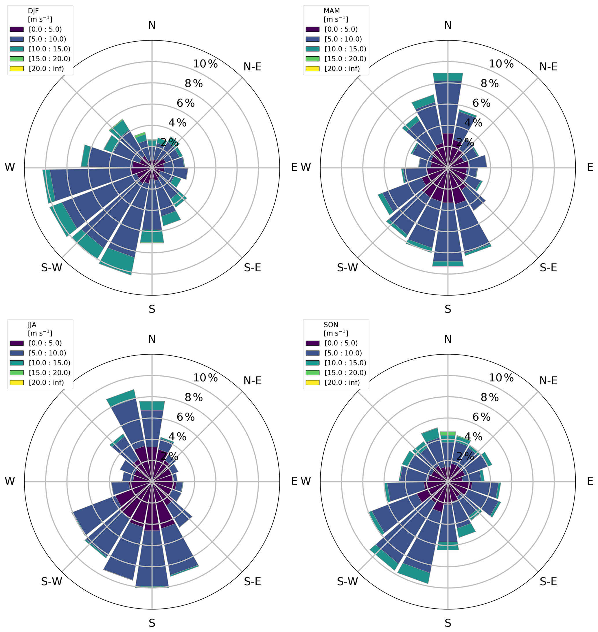
Figure 9 Seasonal wind roses in December 2012–November 2017, drawn from the ERA5 winds at the location of Märket weather station. Please note that wind roses indicate the direction where the wind is blowing from.

3.3 Volume transports in the Åland Sea

To better understand water exchange in the Åland Sea, we analysed volume transports along six zonal (west–east) sections across the basin (locations shown in Fig. 1). For this analysis, transports were integrated over the upper part of the water column down to 40 m depth, over the lower part of the water column below 40 m depth and over the whole water column. This roughly split the water column into an upper (and intermediate) layer above the halocline and a deep layer below the halocline (cf. Sect. 3.2.1). While the depth of the halocline varies somewhat spatially and temporally, the salinity profiles and ADCP data suggest that 40 m is a reasonable estimate for this analysis. As our main interest is in the sub-halocline deep-water transports, and as analysis of currents revealed some significant current speeds in the model layers just below the halocline, we deemed it was more important to choose a separating depth for the analysis that for the most part was either at the halocline or slightly above it.

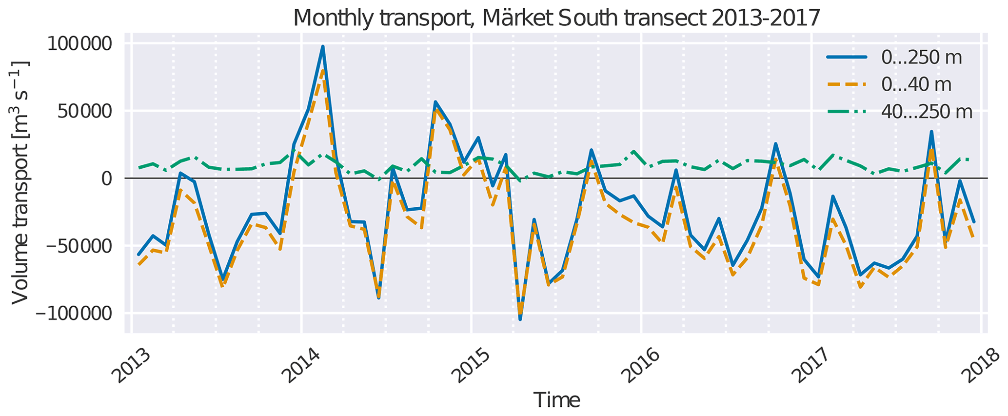
Figure 10 Time series of modelled monthly mean volume transports through the Märket south transect near the northern edge of the Åland Sea 2013–2017. Positive values indicate northward transport. Values for the whole water column, the upper water column up to 40 m and the lower water column below 40 m are shown.

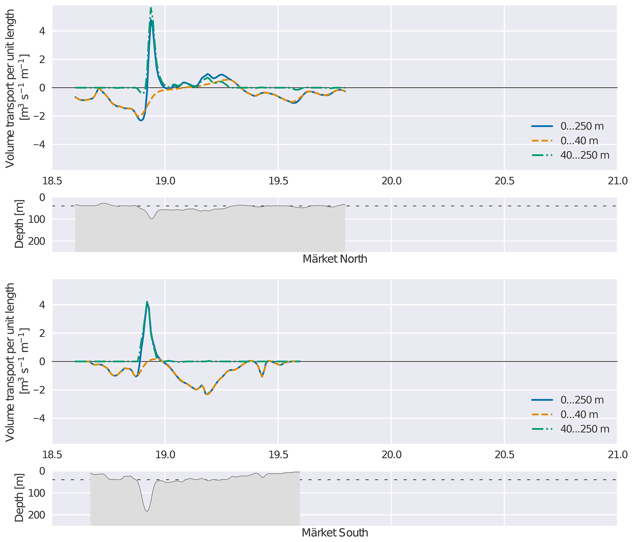
Figure 11 Volume transports per unit length along a transect, integrated over depth, from two northernmost longitudinal transects in the Åland Sea (MN and MS). Mean values for 2013–2017 shown. Positive values indicate northward transport. Values for the whole water column, the upper water column up to 40 m and the lower water column below 40 m are shown. In addition, for each transect a depth profile along the transect is displayed, with the 40 m threshold marked with a dashed line. For reference, 1^∘ longitude is here approximately 55 km in length.

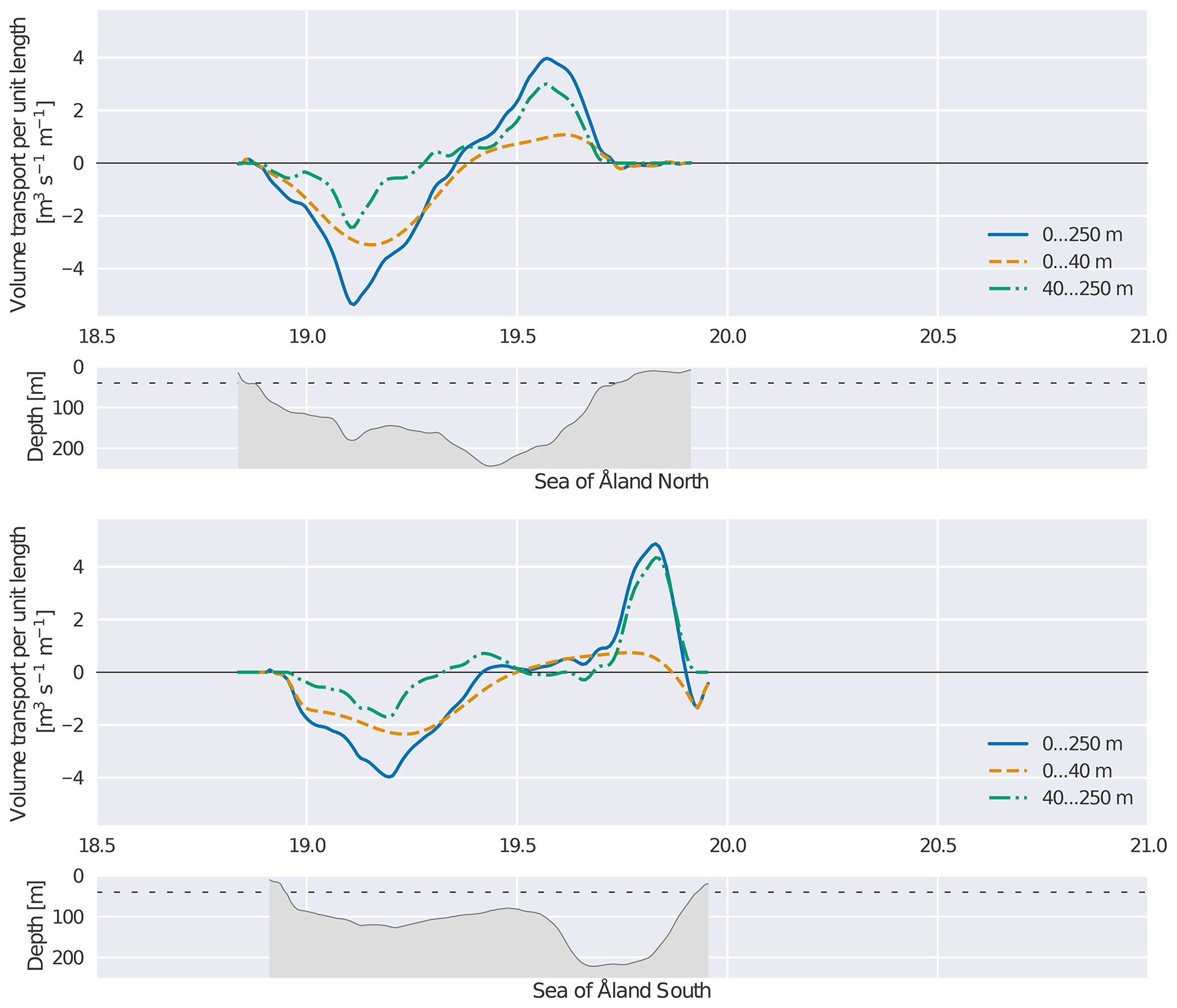
Figure 12 The same as Fig. 11 but for the two transects in the middle part of the Åland Sea (ÅN and ÅS).

Figure 13 The same as Fig. 11 but for the two southernmost transects (LN and LS).

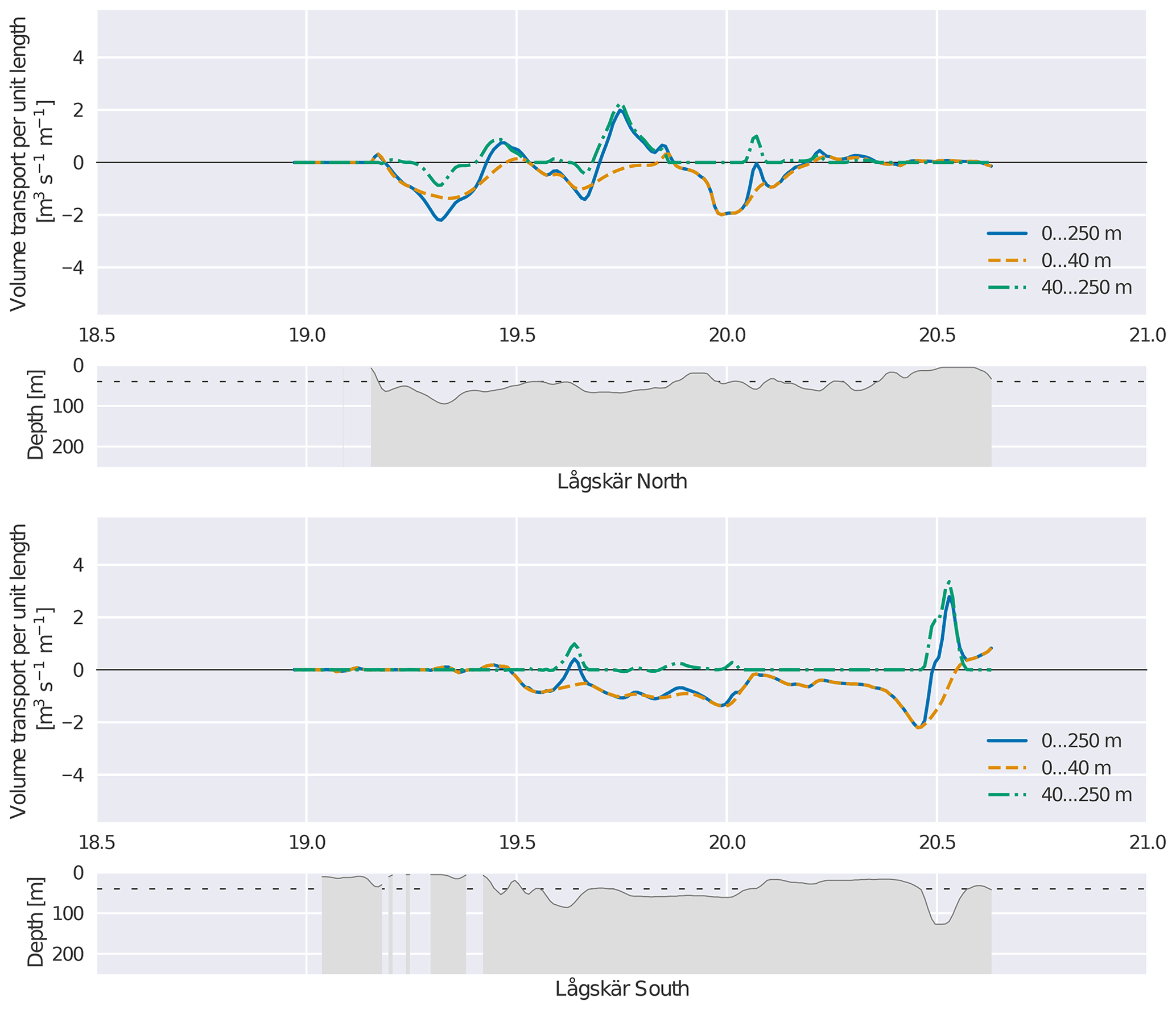
The locations of the transects (see Fig. 1) were chosen to support the aim to study the deep-layer transports in particular. Starting from the north, the two northernmost transects were set north from Märket and Understen and close to them on both sides of the sill to capture fluxes across the Northern Åland Sill. The third and fourth transects represent approximately the middle and southern part of the Åland Sea proper to explain the internal dynamics of the Åland Sea. The fifth and sixth transects are located at the northern and southern edge of the Lågskär Deep to investigate transports in and out of this area in order to explain the role of the Lågskär Deep in the water exchange and eventually in the mixing processes of waters coming from the Baltic proper.

A time series of monthly mean volume transports integrated over the whole transect is shown for the Märket South transect in Fig. 10. While this time series plot is shown here for one transect only, the other transects also show monthly values that are generally of the same order as the ones in this Figure. In the upper layer and for the whole water column, the time series for different transects were highly correlated. For example, when comparing the upper-layer time series for the MS and LS transects, the correlation coefficient was 0.96. For the lower layer, there was more variance in the monthly values between transects, and correlation is weaker when transects are further apart.

An overview of the modelled transports is consistent with the general knowledge of the water exchange in the area. The deep-layer transport goes to the north, and the upper-layer transport goes on average to the south. Transport in the upper layer is much larger than in the lower layer and it dominates the integrated transport. This can be expected, as water entering the Gulf of Bothnia from the south must at some point also exit the gulf towards the south and net precipitation (precipitation minus evaporation) in this area is close to zero or slightly positive (cf. Rutgersson et al., 2001). Furthermore, fresh river runoffs into the Gulf of Bothnia leave the basin in the surface waters, further increasing the surface transport towards the south. There were, however, months when the overall transport is towards the north, most notably in autumn. The largest values of water transport towards the south occurred in late spring and early summer.

Variability from single month to another and single year to another is significant. The mean volume transports for the MS transect for the whole modelling period were −24 000 m³ s⁻¹ (whole water column), −33 000 m³ s⁻¹ (upper layer) and 9200 m³ s⁻¹ (lower layer). It is important to note, however, that the high variability of transports means that the mean transports are very sensitive to the choice of the calculation interval. For example, if we had decided to leave the somewhat anomalous years 2013 and 2014 out of the calculation for the volume transports, the means for the whole water column would have been 30 %–40 % higher. The lower variability of the lower-layer transport means it is much less sensitive to the choice of the averaging interval (difference in this case under 6 %).

Next, to illustrate the pathways of water, we calculated volume transports per unit length along these six sections (Figs. 11–13). Mean values were calculated for the whole study period. Starting now from the south and moving towards the north, waters enter the deep layer in the Lågskär Deep from the Baltic proper mainly across the Southern Åland Sill through the passage starting east of Bogskär (located south of the southern edge of our domain) and connecting to the south-east corner of the Lågskär Deep. The water then is transported to the Åland Sea proper mainly over the Åland Sea Middle Sill between Söderarm and Lågskär.

In the Åland Sea proper, we see a structure where waters flow northwards in the eastern side of the basin and southwards in the western side of the basin. Unlike for the other parts of the Åland Sea, in this case there is also clear southwards transport in the lower part of the water column in the western part of the transect. This is in line with the loop visible in this area in Fig. 7. As the eastern part of the basin is much deeper than the western part, the transport below 40 m is also much larger in the east than in the west. Finally, for the northernmost parts we see deep water flowing northwards between Understen and Märket over the Northern Åland Sill to the Southern Quark Strait.

These transects also reveal some interesting details about the transports. For example, in the southernmost transect we see that, in addition to the strait located at approximately 20.5^∘ E, some deep water also enters the basin through the depression at 19.6^∘ E at the south-west corner of the Lågskär Deep. The primary route is on average responsible for 75 % of the transport. The rest flows through the western parts of the transect.

Furthermore, at the northern edge of the Lågskär Deep, the deep-water transport is divided through three different routes. Transport through the passage east of Lågskär at approximately 20.1^∘ E seems minor when compared to the transport west of Lågskär and east of Söderarm between 19.3 and 20.0^∘ E. Between Lågskär and Söderarm, deep water can take two different routes, and our model indicates that the majority of flow takes place through the eastern route at approximately 19.7^∘ E.

4 Discussion

We built the modelling configuration presented here in part to improve aspects of the system used by Tuomi et al. (2018) and Miettunen et al. (2020) for the Archipelago Sea. First and foremost this means the inclusion of the Åland Sea in the model domain, which made it possible to study water exchange in this area. This is the first study of these exchange processes at such high resolution. Our results are mostly consistent with earlier understanding, with some new details and insights of water exchange processes in the area. The results presented herein are useful for purposes such as planning future ocean observation and marine monitoring activities.

4.1 Currents and circulation

Investigation of currents revealed that the model could capture the overall layered structure of currents reasonably well and the model results were plausible. The two-layer structure of currents (or sometimes even three-layer when a seasonal thermocline was present) observed in the ADCP measurements was well represented in the modelled currents. The model was also able to represent the depth of the halocline that separates these two layers quite reliably.

There are some instances where the direction distribution of the modelled currents somewhat differed from the observations at the ADCP station. Notably, the model showed a larger fraction of relatively low-speed northward currents in the upper layers at the ADCP measurement point than was actually observed. It is worth discussing this difference briefly, as it is related to the reliability of transport estimates in the upper layer. It seems that this difference can in large part result from the inevitable inaccuracies in the placement or timing of submesoscale features in the model. Our model data shows that the circulation field in the Southern Quark area is spatially highly variable with a number of eddies and vortices. Small differences in the locations with submesoscale eddies, for example, can result in significant differences in the direction distribution of currents at a single point if that point ends up on the opposite sides of a current loop in the model and in nature.

Our investigation revealed that in our dataset almost all cases where there were northwards currents in the model and different directions in the observations were times of turbulent and variable circulation field in the model and relatively low current speeds in the vicinity of the ADCP site. Quite often the model current field showed a relatively strong meandering northward mesoscale current east of the ADCP site and an abundance of short-lived submesoscale structures with lower current speeds on both sides that could perhaps be described as “submesoscale soup” (McWilliams, 2019). The model also showed many cases where upper-layer northward currents were modelled well.

Conclusive investigation of these differences would require better spatial coverage of ADCP measurements. For our study period, we only have data from one ADCP station in this area at our disposal. The location of this ADCP was selected to measure currents in the deep layer in the passage between the Åland Sea and the Bothnian Sea, but for validating surface-layer currents a southward location would be better.

Some other sources also support the notion that incorrectly placed submesoscale features and spatial variability might be a significant contributor to these kinds of differences in the direction distribution. For instance, Ehlin and Ambjörn (1977) measured currents at four stations in the Southern Quark. Their current measurement stations were located a couple of kilometres apart. They found that at times current directions could be completely opposite from one station to another, indicating similar spatial variability to what we saw in our model results. It is also prudent to point out that the boundary of our model domain is relatively close to the Southern Quark area. As this is the case, it is possible that inaccuracies – even small ones – in the boundary condition data are reflected in the locations of eddies in the model. In addition, any inaccuracies in wind forcing can be significant.

It is also worth mentioning that gaps in the ADCP measurement record can complicate their interpretation. It is possible that some northward currents could have gone unrecorded. On average, 33 % of all ADCP measurements were missing in the surface layer, with some months lacking up to 77 % of measurements due to measurement difficulties. However, based on our data we estimate that northward currents have not disproportionately gone unrecorded, and this is not a major contributor to this issue.

Investigation of modelled seasonal surface circulation patterns in the Åland Sea revealed an overall structure where southwards currents could be observed throughout the Åland Sea, with the strongest currents along the western edge of the basin. The magnitude of this current varied from one season to another, but the direction was more or less the same. As far as the other parts of the study area are concerned, there was more variability in the direction of the mean current near the southern and northern edge of the area. There were also two cases during the investigation period, winter 2013–2014 and autumn 2014 when the overall direction of the mean seasonal current was towards the north. As expected, near-bottom currents were much less volatile and had less variability than surface currents.

While seasonal means are useful for many applications, care should be taken when they are applied. It is important, for example, to remind ourselves that there is a lot of variability in the circulation patterns at shorter timescales that is hidden by the averaging process (cf. Westerlund, 2018). Near-surface circulation patterns are especially affected by wind forcing, for instance. Averaging current vectors for seasons with lower persistency, namely autumn, results in much lower mean speeds than averaging current magnitudes with no consideration for their direction.

4.2 Volume transports

The overall picture of modelled water exchange in the Åland Sea mostly followed what has been reported earlier. More saline water from the Baltic proper enters the Åland Sea mostly through Lågskär Deep, after which it is transported northwards through the Åland Sea proper, ultimately reaching the Bothnian Sea through the Southern Quark. However, it was interesting that in our model only 75 % of the water that enters from the Baltic proper in the deep layer is transported through the primary route in the south-east corner of Lågskär Deep, while a significant percentage bypasses the Lågskär Deep entirely from its western side.

It is somewhat challenging to find an appropriate frame of reference for our water transport results from the literature. Previous estimates of water exchange through the Åland Sea and the Archipelago Sea have often employed a Knudsen type budget approach (Knudsen, 1900). As Myrberg and Andrejev (2006) note, there is significant variance between the results of different studies depending on factors such as averaging period, temporal coverage of measurements and location of transects in relation to dynamical features. Furthermore, these estimates are typically for the whole Gulf of Bothnia, while we concentrate on the Åland Sea and leave the Archipelago Sea for future studies. Therefore, as the water exchange through the Archipelago Sea is not included in our estimates, we should look at these previous results more as upper bounds. Myrberg and Andrejev (2006) point out that these estimates can nevertheless be compared to modelling results as the first approximation.

Ambjörn and Gidhagen (1979) give estimates for net water transport in the Åland Sea. Values for monthly transports for a few months in the late 1970s are reproduced in Table 1. These numbers are based on current measurements and empirical orthogonal functions (EOF). While there is notable inter-annual variability in transports and these values cannot be directly compared to our results, looking at our Fig. 10 we see that the direction (southwards) is the same, as is the general magnitude in the latter half of the year (approximately from zero to −10⁵ m³ s⁻¹).

Table 1 Net water transport in the Åland Sea according to Ambjörn and Gidhagen (1979). The last column has been calculated assuming 30.437 d per month.

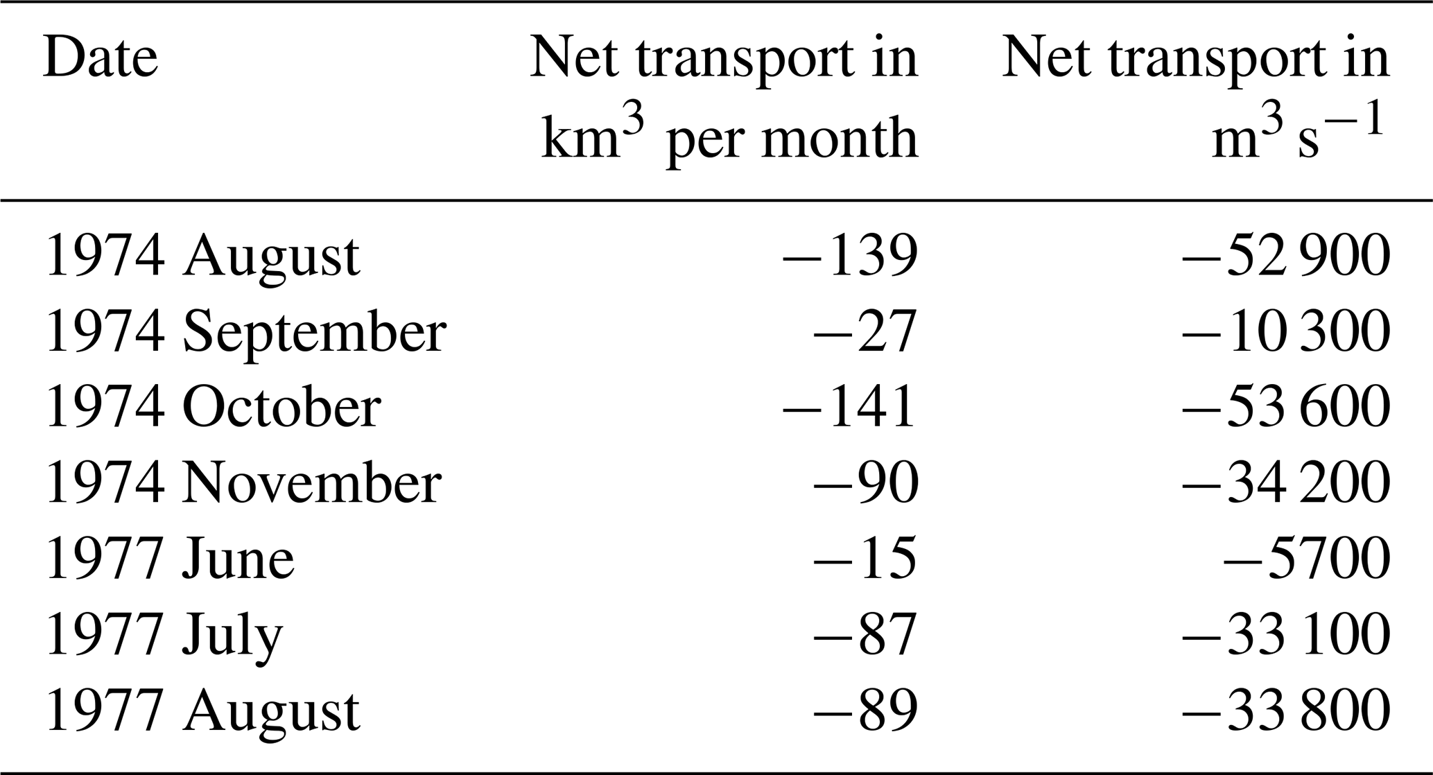
Ehlin and Ambjörn (1977) also published estimates of water transport to the Gulf of Bothnia, partially based on the same data as Ambjörn and Gidhagen (1979). They used tide gauge data from the Gulf of Bothnia and current measurements from several stations in the Understen-Märket area in 1973–1974. When they investigated daily mean transports in the area, they arrived at values that varied mostly between 5 and 10 km³ d⁻¹, which translates approximately to 58 000–120 000 m³ s⁻¹. They also saw much higher values, which is expected as they recorded daily transports.

Our modelled values from the same area in Fig. 10 mostly fall within the range of values given by both Ambjörn and Gidhagen (1979) and Ehlin and Ambjörn (1977). This builds confidence for using the modelling approach in these types of studies.

The veracity of modelled transports depends heavily on how well the model captures magnitudes and directions of current fields. The ADCP validation suggests that modelled currents are mostly trustworthy (at least near the ADCP station). This in turn would suggest that the overall magnitude of transports could be reasonable. As discussed, the model seems to indicate a somewhat greater fraction of northward currents in the surface layer than is present in observations, which might mean that in some cases the surface-layer volume transport would perhaps be overestimated. However, an investigation of such cases revealed that current magnitudes were mostly moderate. Cases where the model simulates the dynamical situation completely incorrectly seem to be very rare. In the period when ADCP observations were available, August 2016–December 2017, the most notable case was in October 2016. As in this month we had stronger northward currents in the model than in the ADCP data, it suggests that we should treat the positive value for surface-layer volume transport for that month in Fig. 10 as an upper limit. While it stands to reason that the modelled upper-layer transport may overall be somewhat more uncertain than in the deep layer, other differences in this validation were less major. If ADCP measurements with better spatial and temporal coverage became available, they could clarify this issue further. In addition, it would be useful if future current measurements could reliably capture currents in the whole water column even in deeper areas.

4.3 Model configuration and parameterizations

Because of the diverse bathymetric and hydrographic features of our study area, one of the key challenges for this study was finding the right balance between model stability and mixing. A notable difference with the configuration by Tuomi et al. (2018) was our choice of the z^∗ vertical coordinate system instead of σ coordinates.

While the σ coordinate system is highly popular in coastal modelling applications, it has some issues that make it less ideal for the Åland Sea–Archipelago Sea area. One of these issues is the presence of the internal pressure gradient error. It can be especially problematic for coastal problems that include steep bathymetric gradients such as canyons or seamounts (Fringer et al., 2019). For many coastal problems, where strong tidal currents and mixing dominate, the internal pressure gradient error is a minor issue. However, the Baltic Sea is micro-tidal, and thus for our study area this issue is potentially relevant. Indeed, Tuomi et al. (2018) found significant over-mixing, especially in the deeper channels of the Archipelago Sea.

One way to address this issue is to use geopotential coordinate systems, which do not exhibit the pressure gradient error. Unfortunately, these systems have their own problems. For example, the standard geopotential vertical coordinate system limits the size of the topmost vertical level, which makes it more difficult to study near-surface dynamics (Klingbeil et al., 2018). This issue can be resolved by the use of the z^∗ system, which allows finer vertical resolution.

A considerable amount of manual work was required to ensure that bathymetric features of the area were represented in the model grid as accurately as possible, so that instabilities were not introduced by bathymetric artefacts appearing due to the limited grid resolution. At the same time, we had to find values for mixing parameters that produced reasonable results while simultaneously being high enough to maintain model stability.

The end result is satisfactory in the sense that this model configuration seems to be able to reproduce even strong gradients quite well and does not suffer from spurious over-mixing to the same extent as the configuration by Tuomi et al. (2018). Still, it is evident that further tuning of model bathymetry, bottom friction and mixing parameters would be beneficial to improve results further. Depending on the scales and phenomena that are investigated with this configuration in the future, higher-resolution forcing data might also be useful.

One limiting factor for model accuracy is that high-resolution bathymetric data from the area either does not exist or is not generally available. Sometimes, the bathymetry simply has not been measured with high enough accuracy, while in other cases the availability of existing data for scientific study is limited by non-scientific factors such as national security concerns or commercial interests. In the future, efforts to make higher-resolution bathymetric data available would make further model improvements possible.

4.4 Outlook

This study is the first step on the way to resolving the open questions relating to water exchange between the Baltic proper and the Gulf of Bothnia. The next steps could include, for example, a closer investigation of transport dynamics and drivers of transport features. In addition, there is still uncertainty regarding the routes and volumes of water in the Archipelago Sea. Longer model runs should be performed to reduce uncertainties of the transport estimates when it is technically possible. Water exchange could be investigated on both longer and shorter time spans, and the role of significant water exchange events could be elaborated. Furthermore, salinity transports are interesting when working to understand connections to the environmental changes in the Bothnian Sea. Including nutrient transports in the analysis would be interesting.

Another possible application for volume transports computed from this configuration could be to compare them to results from a coarser configuration. Many regional Baltic Sea models are unable to fully resolve the Åland Sea area due to limited resolution. State-of-the-art regional configurations nowadays typically have horizontal resolutions of around 1 nmi (see, e.g. Kärnä et al., 2021). Efforts to develop regional configurations further might benefit from such analysis.

Further developments of the modelling configuration could improve its accuracy. For example, boundary conditions can have a major impact on the results. For instance, salinity biases present in the boundary conditions can be quickly propagated to the whole modelling area. One possible way to address these issues could be the development of an improved configuration for the area with two-way nesting.

In addition to water exchange and transports, this modelling configuration could also be used to investigate a number of other topics, some of which we mention here. Questions related to the environmental health of the sea and nutrient reductions could be studied. This configuration could, for example, provide current fields to nutrient load modelling in a similar manner as the COHERENS-based model configuration used by Lignell et al. (2018). The relatively high resolution could also allow studies of coastal processes with detail and spatial coverage that so far has not been possible. Furthermore, this configuration might prove useful for assisting marine spatial planning, for example by providing data for studies of connectivity of marine habitats. In addition, substance transport modelling is a topical issue that could be supported with this setup. Both Lagrangian and Eulerian transport studies could be interesting and could be conducted either by adding an online component to this configuration or by coupling another model offline for substance transport in a similar manner to Miettunen et al. (2020).

5 Conclusions

We studied volume transports through the Åland Sea in the Baltic Sea with a new high-resolution hydrodynamic model configuration.

Investigation of modelled current magnitudes and distribution in the area provided encouraging results regarding the ability of our configuration to capture the overall dynamics and volume transports in the Åland Sea. We found that modelled circulation patterns in the study area were variable. Currents typically had a two-layer structure separated at the halocline. Seasonal means revealed that there commonly was a southward current in the surface layers in all seasons. The stability of currents was notably lower in autumn compared to other seasons. In the deeper layer, currents were directed by bathymetric features and mostly towards the north for all seasons.

Analysis of modelled volume transports showed how deep water is transported northward from the Baltic proper to the Bothnian Sea over the sills and via the available passages. Time series of volume transports from the northern Åland Sea revealed that monthly averages of deep transport were consistently towards the north. On the surface, the net transport was towards the south. However, in most years there were months in late summer or early autumn with northward monthly mean transports in the surface layer.

Our analysis indicates that the dynamics in Lågskär Deep are more complex than has previously been thought. It seems that while Lågskär Deep is the primary route of deep-water exchange, a significant volume of deep water still enters the Åland Sea through the depression west of the Lågskär Deep. The primary route is on average responsible for 75 % of the transport, while the rest flows through the western parts of the transect.

Future studies of transport and nutrient dynamics will eventually enable a deeper understanding of eutrophication changes in the Gulf of Bothnia. In future studies, the reliability of current and transport estimates could be improved with increased spatial and temporal coverage of current observations from this area. While the configuration reproduced the overall temperature and salinity dynamics and sea surface heights in the area in an adequate manner, model validation would further benefit from CTD datasets with good spatial and temporal coverage. High-quality forcing and boundary condition datasets would also help to build further confidence in the water exchange estimates.