the Creative Commons Attribution 4.0 License.
the Creative Commons Attribution 4.0 License.
 | 20 Oct 2020
Connecting flow–topography interactions, vorticity balance, baroclinic instability and transport in the Southern Ocean: the case of an idealized storm track
Xavier Capet
The dynamical balance of the Antarctic Circumpolar Current and its implications on the functioning of the world ocean are not fully understood and poorly represented in global circulation models. In this study, the sensitivities of an idealized Southern Ocean (SO) storm track are explored with a set of eddy-rich numerical simulations. The classical partition between barotropic and baroclinic modes is sensitive to current–topography interactions in the mesoscale range 10–100 km, as comparisons between simulations with rough or smooth bathymetry reveal. Configurations with a rough bottom have weak barotropic motions, ubiquitous bottom form stress/pressure torque, no wind-driven gyre in the lee of topographic ridges, less efficient baroclinic turbulence and, thus, larger circumpolar transport rates. The difference in circumpolar transport produced by topographic roughness depends on the strength with which (external) thermohaline forcings by the rest of the world ocean constrain the stratification at the northern edge of the SO. The study highlights the need for a more comprehensive treatment of the Antarctic Circumpolar Current (ACC) interactions with the ocean floor, including realistic fields of bottom form stress and pressure torque. It also sheds some light on the behavior of idealized storm tracks recently modeled: (i) the saturation mechanism, whereby the circumpolar transport does not depend on wind intensity, is a robust and generic attribute of ACC-like circumpolar flows; (ii) the adjustment toward saturation can take place over widely different timescales (from months to years) depending on the possibility (or not) for barotropic Rossby waves to propagate signals of wind change and accelerate/decelerate SO wind-driven gyres. The real SO having both gyres and ACC saturation timescales typical of our “no gyre” simulations may be in an intermediate regime in which mesoscale topography away from major ridges provides partial and localized support for bottom form stress/pressure torque.
- Article
(10693 KB) - Full-text XML
- BibTeX
- EndNote


The strength of the Antarctic Circumpolar Current (ACC) is controlled at first order by a balance between the eastward momentum imparted by the persistent Southern Ocean (SO) winds and the topographic form stress at the ocean bottom (Munk and Palmén, 1951; Hughes and de Cuevas, 2001). The bulk of the bottom pressure gradients is thought to be provided at the major submarine ridge (Kerguelen Plateau, Macquarie Ridge, Scotia Arc and East Pacific Rise) and the South American continent (Munk and Palmén, 1951; Gille, 1997; Masich et al., 2015).
Along with their decelerating action on the mean flow, the major ridges result in strong inhomogeneity of the SO dynamics. Indeed, they act to concentrate and energize the eddy activity downstream of the topography, in regions often referred to as “storm tracks”. The underlying process is a local intensification of the baroclinicity and baroclinic instability of the flow (Bischoff and Thompson, 2014; Abernathey and Cessi, 2014; Chapman et al., 2015). Localized baroclinic instability goes in hand with a suppression of eddy growth away from the ridge (Abernathey and Cessi, 2014). Overall, ridges profoundly shape the SO dynamics, stratification (Abernathey and Cessi, 2014; Thompson and Naveira Garabato, 2014) and subduction hotspots (Sallée et al., 2010).
Another potentially important aspect of the dynamics through which ridges affect the SO circulation is the formation of closed recirculating gyres driven by Sverdrup-like dynamics that coexist with the circumpolar flow (Tansley and Marshall, 2001; Jackson et al., 2006). From idealized numerical simulations of the ACC, it was recently highlighted by Nadeau and Ferrari (2015) that increasing wind intensity leads to increasing gyre circulation without modification of the circumpolar transport, suggesting that the saturation of the circumpolar transport with increasing winds may be connected with gyre dynamics. Patmore et al. (2019) further highlighted that ridge geometry is important for determining gyre strength and the net zonal volume transport.
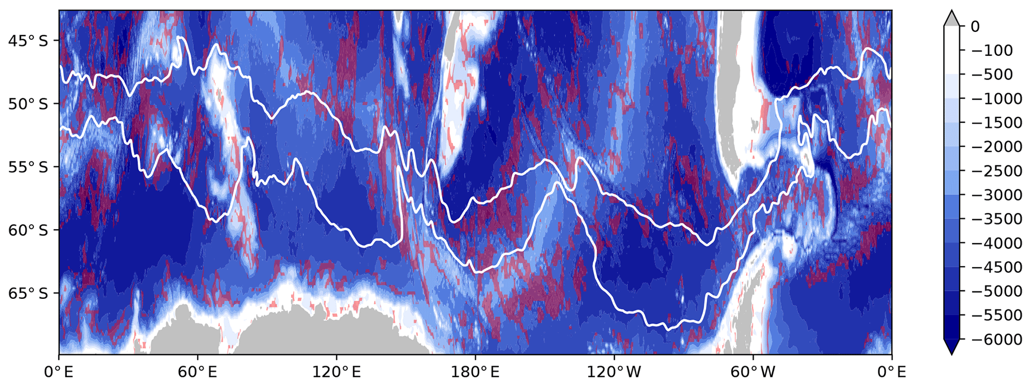
Figure 1Topography (m) of the Southern Ocean from ETOPO2 (National Geophysical Data Center, NOAA). The red dashed areas indicate areas with a topographic roughness (computed as the variance in the topography over an area of 100 km×100 km as in Wu et al., 2011) between 3×10⁴ and 105 m2. The main pathway of the ACC is identified by two isocontours (0.4 and 1 m) of mean dynamical topography from AVISO.
Apart from the major ridges (Fig. 1), the seafloor is shaped by topographic features with horizontal scales from hundreds of meters to tens of kilometers (mainly abyssal hills), which are thought to dissipate most of the large-scale wind power input in the SO through the generation of internal lee waves (Nikurashin and Ferrari, 2011) and to provide high abyssal mixing (Nikurashin and Ferrari, 2010a). But a substantial fraction of the bottom topography variance is also contained at scales in between the major ridges (100 km and larger) and the typical width scale of the abyssal hills (O 1–10 km; see Goff and Jordan, 1988; Nikurashin and Ferrari, 2010b). This range of topographic scale between 10 and ∼100 km will be referred to as “mesoscale” and is in part associated with the abyssal hills (e.g., Goff and Arbic, 2010)1. The influence of mesoscale topography on SO dynamics is expected to be of second order because they are less effective than large-scale ridges at arresting the time-mean ocean circulation through form stress (Naveira-Garabato et al., 2013; see also Tréguier and McWilliams (1990) for numerical evidence of this).
Using zonally re-entrant channel simulations with a meridional ridge, this study investigates the sensitivity of an idealized SO storm track to the presence or absence of mesoscale topographic irregularities, a case that has not been investigated in Treìguierand McWilliams (1990). Surprisingly, our results show that the form stress exerted by the mesoscale topography has a major influence on the ACC transport, albeit indirectly. How this influence plays out in different settings is explored via sensitivity runs to the model northern boundary restoring (i.e., to the nature of the coupling between the SO and the rest of the word ocean) and wind strength. Unpacking the causes of the rough topographic influence sheds some light on the key processes that structure the SO circulation, namely flow–topography interactions and their potential control over the barotropic flow and waves, the form stress and its role in the vorticity balances, and the baroclinic instability. The numerical experiments are presented in Sect. 2. Section 3 is focused on the description of diagnostics for the dynamics in our different sensitivity runs. In Sect. 4, we combine these “pieces of the puzzle” and attempt to compose a unified dynamical interpretation of our results in the form of a causal chain of elementary processes. Concluding remarks are given in Sect. 5.
2.1 The numerical setup
The numerical set up consists of a periodic channel configuration of 4000 km long (Lx, zonal direction) and 2000 km wide (Ly, meridional direction), with walls at the northern and southern boundaries. It is inspired from the simulations described in Abernathey et al. (2011) and Abernathey and Cessi (2014), and it aims to represent a zonal portion of the SO (Fig. 2).
The numerical code is the oceanic component of the Nucleus for European Modeling of the Ocean program (NEMO; Madec, 2014). It solves the three-dimensional primitive equations discretized on a C-grid and fixed vertical levels (z coordinate). Horizontal resolution is 5 km. There are 50 levels in the vertical, with 10 levels in the upper 100 m and cell thickness reaching 175 m near the bottom. Precisely, the thickness of the bottom cells is adjusted to improve the representation of the bottom topography, with a partial step thickness set larger than 10 % of the standard thickness of the grid cell. The model is run on a β plane with s−1 at the center of the domain and m−1 s−1 the derivative of the planetary vorticity. A third-order upstream biased scheme (UP3) is used for both tracer and momentum advection, with no explicit horizontal diffusion (implicit diffusion can be diagnosed whenever necessary; see for instance Jouanno et al., 2016). The vertical diffusion coefficients are given by a generic length scale (GLS) scheme with a k–ε turbulent closure (Reffray et al., 2015). Bottom friction is linear with a bottom drag coefficient of m s−1 and is computed based on an explicit formulation. The free surface formulation is linear and uses a filtered free-surface scheme (Roullet and Madec, 2000). We use a linear equation of state with temperature as the only state variable and a thermal expansion coefficient K−1. The temporal integration involves a modified leap-frog Asselin filter, with a coefficient of 0.1 and a time step of 400 s.
The forcing consists of an eastward wind defined as
with U0=10 m s−1. The wind stress is calculated using the formulation from Large and Yeager (2009). This leads to a maximum wind stress of 0.14 N m−2 at Ly∕2 and zero wind stress curl at the northern and southern walls.
At the northern boundary, the model can be restored toward an exponential temperature as motivated by observations (Karsten and Marshall, 2002) and following the formulation proposed in Abernathey et al. (2011):
with ΔT=8 ∘C, H=4000 m the depth of the domain and h=1000 m. The relaxation coefficient varies linearly from 0 at y=1900 km to 7 d at Ly.
The surface heat flux Qair-sea is built using a relaxation method toward a prescribed sea surface temperature (SST) climatology. It depends on a sensitivity term γ set to 30 W m−2 K−1 (Barnier et al., 1995) and on the difference between Tmodel and a predefined climatological SST field Tclim:
with .
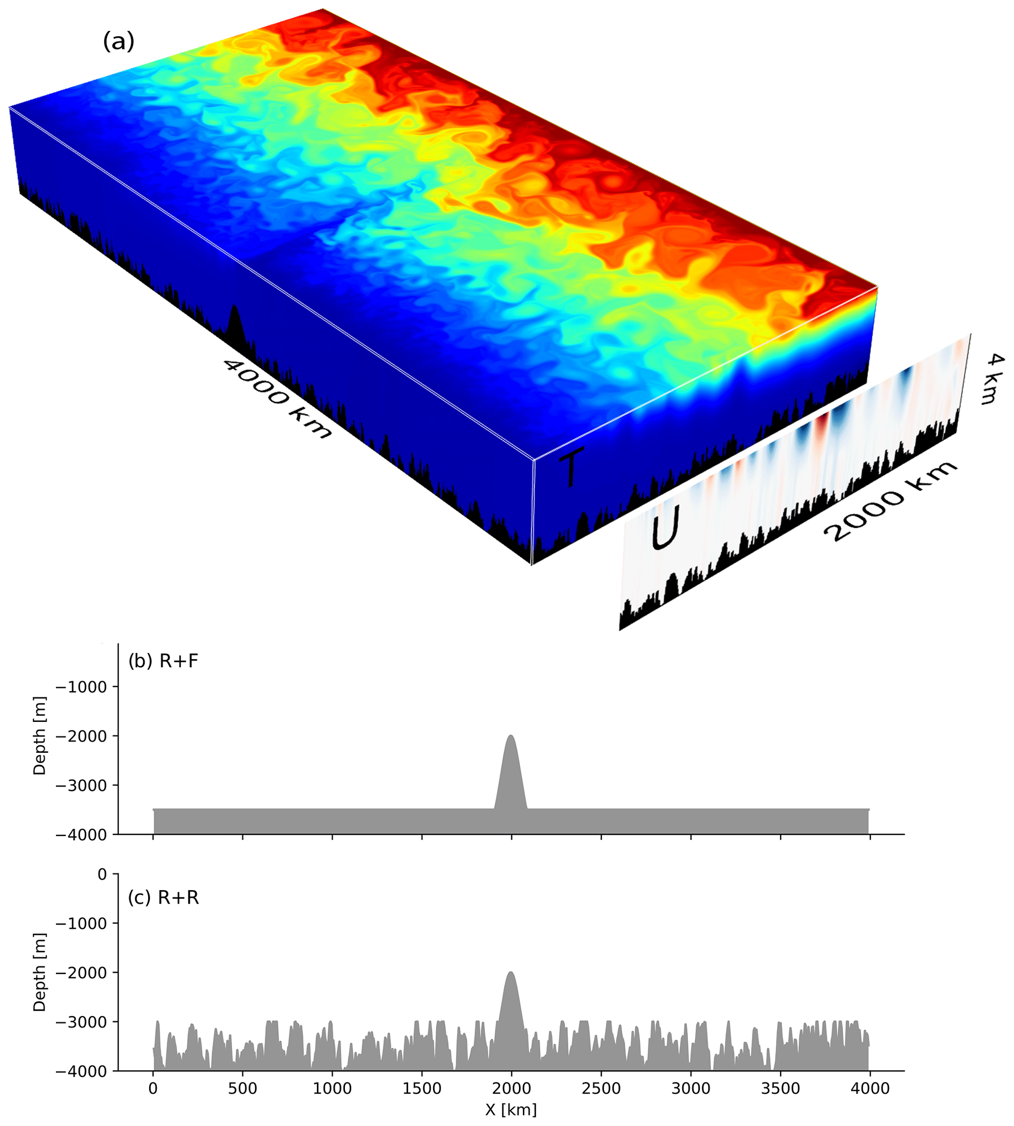
Figure 23D representation (a) of instantaneous temperature (rectangular box, color scale ranges from 0 to 8 ∘C) and zonal velocity (vertical section) for the simulation R + R after 200 years. The domain is a 4000 km long by 2000 km wide re-entrant channel. The maximum depth is 4000 m with irregular bottom topography bounded at 3000 m and a Gaussian-shaped ridge of 2000 m located at x=2000 km, which limits the ACC transport and generates a standing wave downstream as seen in the surface temperature. Topography at y=1000 km in the two simulations: (b) R + F and (c) R + R. The rms height in R + R averaged within 50 km×50 km areas out of the region of the ridge is 250 m.
Simulations have been performed with two types of topography. All include a Gaussian-shaped ridge centered in the middle of the domain (x=2000 km). The height of the meridional ridge is given by , with h0=2000 m the maximum height of the ridge, σ=75 km and H=4000 m the maximum depth of the domain.
2.2 Sensitivity to bottom roughness and northern restoring
We performed two sets of simulations that differ in their bathymetry outside the ridge (Fig. 2b, c). In R + F (for ridge and flat) simulations, the bottom floor outside the ridge is flat and located at 3500 m depth (hrms=0 m). In R + R (for ridge and rough) simulations, the bottom depth outside the ridge varies between 3000 and 4000 m depth with random fluctuations of horizontal wavelength between 10 and 100 km (hrms=250 m) and the constraint that the averaged depth remains 3500 m as in R + F. The bottom roughness, defined as the variance in the bottom height H, is 6.2×10⁴ m2. This choice of roughness and horizontal scales is consistent with the characteristics of some SO topography but not for all the sectors (Fig. 1; see also Wu et al., 2011, or Goff, 2010). The impact of spatially varying roughness is not addressed in this study and would deserve dedicated sensitivity experiments to connect finely with the dynamics of the real Southern Ocean.
Restoring temperature toward a prescribed stratification profile at the northern boundary exerts a strong constraint on the model solution and can partially account for the influence of low-latitude and northern hemispheric ocean sectors. Channel configurations with limited meridional extent have alternatively been using strategies with or without northern restoring (e.g., Abernathey et al., 2011; Abernathey and Cessi, 2014). In order to test the sensitivity of our results to this constraint, we performed additional experiments without restoring, which are referred as R + Fnr and R + Rnr.
The four simulations (R + F, R + R, R + Fnr and R + Rnr) are initialized with the same initial conditions consisting of an ocean at rest and a stratification given by the stratification prescribed at the northern boundary. They are integrated over 150 years. Unless otherwise stated, monthly instantaneous fields from the last 10 years are used for diagnostics. In addition, simulations with increased wind forcing (maximum wind stress of 0.28 N m−2 at ) have been integrated for 30 years, starting from the equilibrium state of the reference set of simulations (forced with maximum wind stress of 0.14 N m−2 as mentioned above).
2.3 Vorticity balance
The barotropic vorticity (BV) balance plays a key role in the analysis of our model runs. The time-mean BV equation reads as follows (see Jackson et al., 2006, and Hugues and De Cuevas, 2001, for physical insight):
with V the integrated time-mean meridional velocity, J(pb,H) the bottom pressure torque – with pb pressure at the seafloor and H the ocean depth – and the nonlinear advection term. The different terms were evaluated by taking the curl of the depth-integrated momentum balance terms computed online. The contributions of the lateral and temporal diffusion are very weak and are not shown.

Figure 3KE (m2 s−2), EKE (m2 s−2) and (m2 s−3) averaged between the surface and 500 m. These fields have been computed using instantaneous monthly data for the last 10 years of the simulation (a–c) R + F and (e–f) R + R.
3.1 Overall characteristics of the simulations
Independently of bottom roughness or northern restoring, the topographic ridge forces a large-scale standing meander in its lee (Fig. 3a, d), as found in previous studies (Abernathey and Cessi, 2014, Nadeau and Ferrari 2015; Chapman et al., 2015). The baroclinic instability of the meander, as revealed by the distribution of vertical eddy buoyancy flux (Fig. 3c, f; with w′ and b′ the vertical velocity and buoyancy anomalies with respect to time-averaged values, the 0–500 m vertical averaging, and the 10-year temporal averaging), energizes the eddy field in the ∼500 km downstream of the ridge (Fig. 3b, e). Further downstream, the energy of the eddies drops off. The resulting EKE distribution is typical of SO storm tracks as described for example in Chapman et al. (2015). The kinetic energy of the mean flow (MKE; Fig. 4a), the eddy kinetic energy (EKE; Fig. 4b), and the marked isopycnal slope in the upper 1000 m (Fig. 5c) all illustrate the strong baroclinic character of the dynamics.
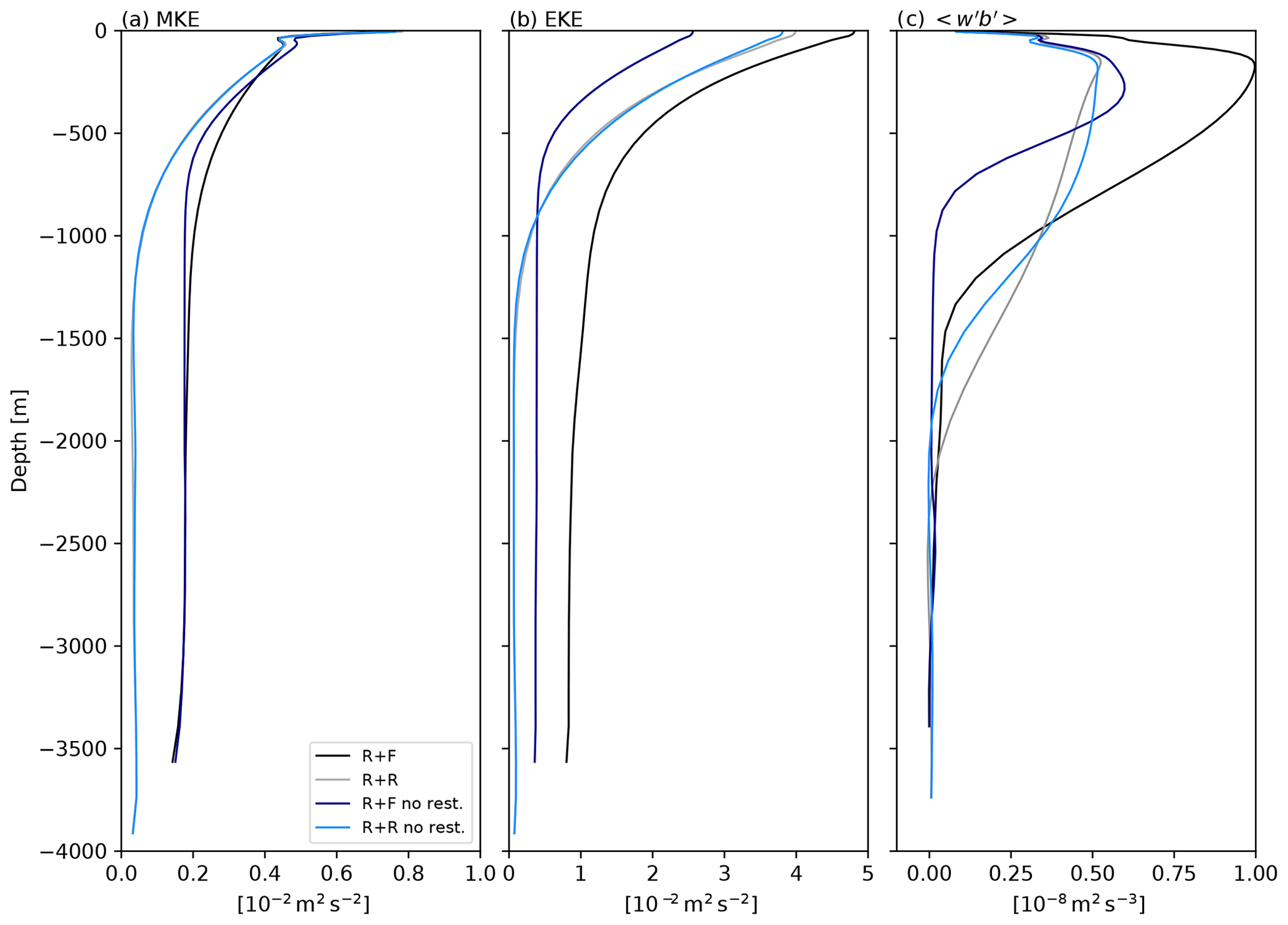
Figure 4Vertical profile of (a) kinetic energy of the mean flow (m2 s−2), (b) eddy kinetic energy (m2 s−2) and (c) the vertical eddy buoyancy flux (m2 s−3) as a signature of baroclinic energy transfer from eddy potential energy to eddy kinetic energy. Diagnostics use the last 10 years of the simulations and were averaged over the full domain in the zonal direction and between y=500 km and y=1500 km in the meridional direction. The velocity (u′, v′, w′) and buoyancy (b′) anomalies use to compute the eddy kinetic energy in (a) and the buoyancy flux in (c) are anomalies with respect to the 10-year temporal mean. The kinetic energy of the mean flow (MKE; a) is computed using 10-year-averaged velocities.
The equilibrium state of the different simulations is almost achieved after 100 years as indicated by the stabilization of the zonal transport and total kinetic energy (KE; Fig. 5a, b)2. The topographic drag of the ridge constrains the zonal flow to transports between 25 and 75 Sv (sverdrups) . These values are weak compared to the barotropic transport obtained for similar channel simulations with a flat bottom (∼800 Sv in Abernathey and Cessi, 2014) or rough topography only (∼300 Sv in Jouanno et al., 2016), but they are in line with configurations with a ridge (∼90 Sv in Munday et al., 2015 or Marshall et al., 2017; ∼60 Sv in Abernathey and Cessi, 2014).

Figure 5The 150-year time series of (a, d) domain-averaged total kinetic energy (units: m2 s−2), (b, e) transport (units: Sv) and (c, f) sections of zonally averaged mean temperature for the last 10 years of the simulations (contours ranging from 1 to 7 ∘C). Simulations with restoring at the northern boundary (R + R and R + F) are shown in (a) and (c), and simulations without restoring (R + Rnr and R + Fnr) are shown in (b) and (d). In (c), the vertical dashed line indicates the limit of the restoring zone at the northern boundary.
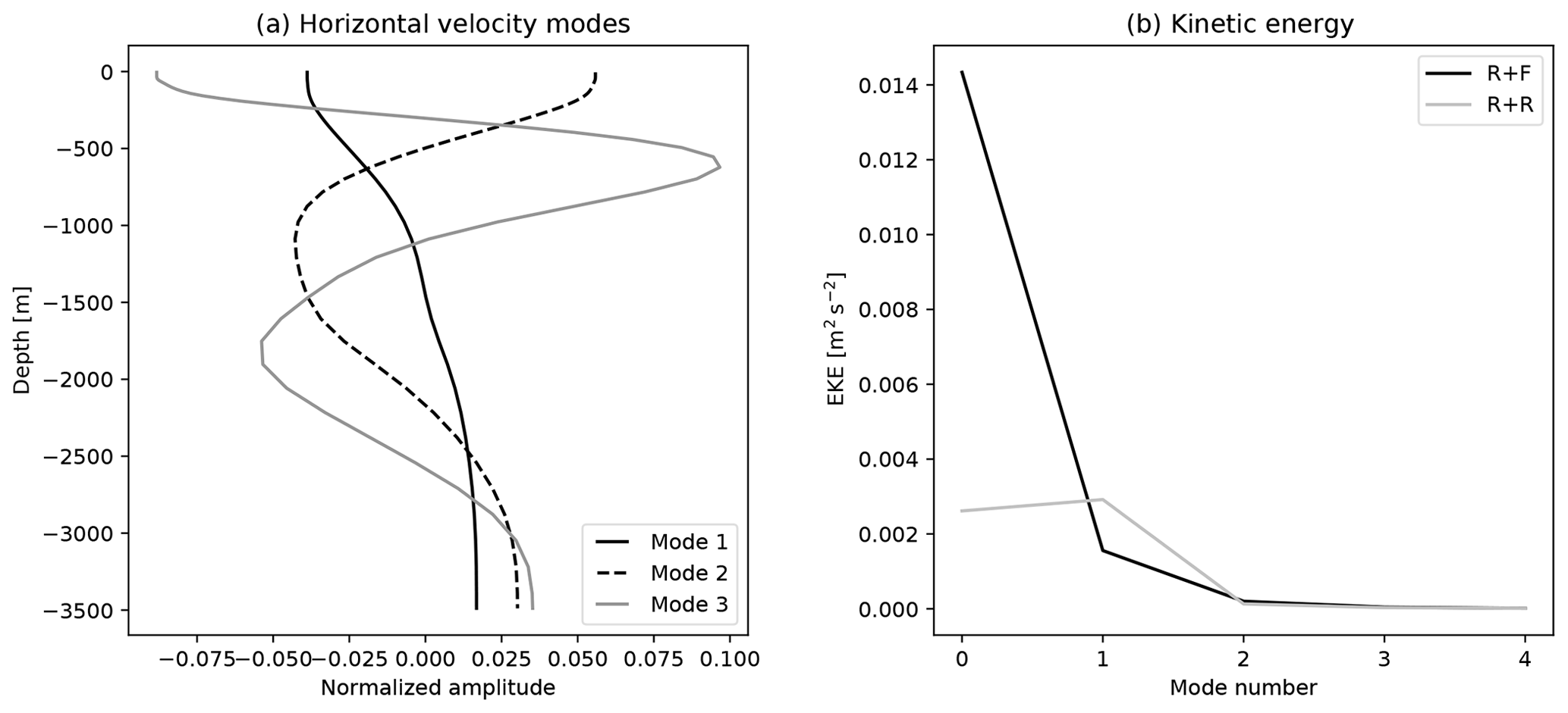
Figure 6Normal mode analysis: (a) the first three baroclinic modes at position (x=0; y=1000 km) for the experiment flat and (b) kinetic energy (m2 s−2) contained in each mode, with mode 0 corresponding to the barotropic mode. The kinetic energy given in (b) results from a combination of, first, spatial averaging over 40 profiles taken at the central latitude (y=1000 km) and regularly spaced in longitude all along the channel and, second, temporal averaging 120 snapshots obtained at monthly frequency over the last 10 years of simulations R + F and R + R.
3.2 Sensitivity to bottom roughness
We now describe the influence of bottom roughness on the channel dynamics. We do this by comparing the main attributes of simulations R + F and R + R side by side. We start with the simulations including northern restoring because their sensitivity to topography is simpler; the northern restoring acts on the density structure so the mean state does not depart too much between the two simulations. The key result is that bottom roughness leads to a ∼60 % increase in the zonal transport (Fig. 5b) from 45 to 72 Sv. These changes of zonal transport are associated with profound modifications of the overall dynamics.
3.2.1 Vertical structure of the flow
The vertical structure of time-mean and transient flow components is very sensitive to bottom roughness. In the latitude range where the ACC is located, the flow is impacted (above 700 m) as revealed by values of MKE and EKE that are larger in R + F compared to R + R (Fig. 4a, b). Most importantly, finite values of MKE and EKE persist below 1000 m in R + F (Fig. 4a, b), indicative of a significant contribution of the barotropic mode, while MKE and EKE are vanishingly small in the deep layers of R + R. This agrees with the modal decomposition carried out at y=1000 km (Fig. 6). The barotropic mode contains most of the energy in R + F, while the energy in R + R is almost evenly distributed between the barotropic and first baroclinic mode.
The spectral analysis in Fig. 7 highlights the profound differences between the two solutions. Near the ocean floor, up to ∼1500 m depth, bottom roughness energizes the flow at wavelengths finer than ∼30 km – a wavenumber of rad m−1. On the other hand, it is responsible for a marked reduction of deep ocean KE at wavelengths larger than ∼30 km, i.e., both at large scale and mesoscale. This directly affects the flow up to 1500 m, i.e., at depths well above the bottom floor (Fig. 7b).
The changes in the vertical structure of the flow can be interpreted as follows: bottom roughness forces the mean and eddy bottom flow to near-zero levels and thus weaken the barotropization process for both the large and mesoscale dynamics. This echoes recent findings by LaCasce (2017) that bathymetric slopes promote surface intensified modes.
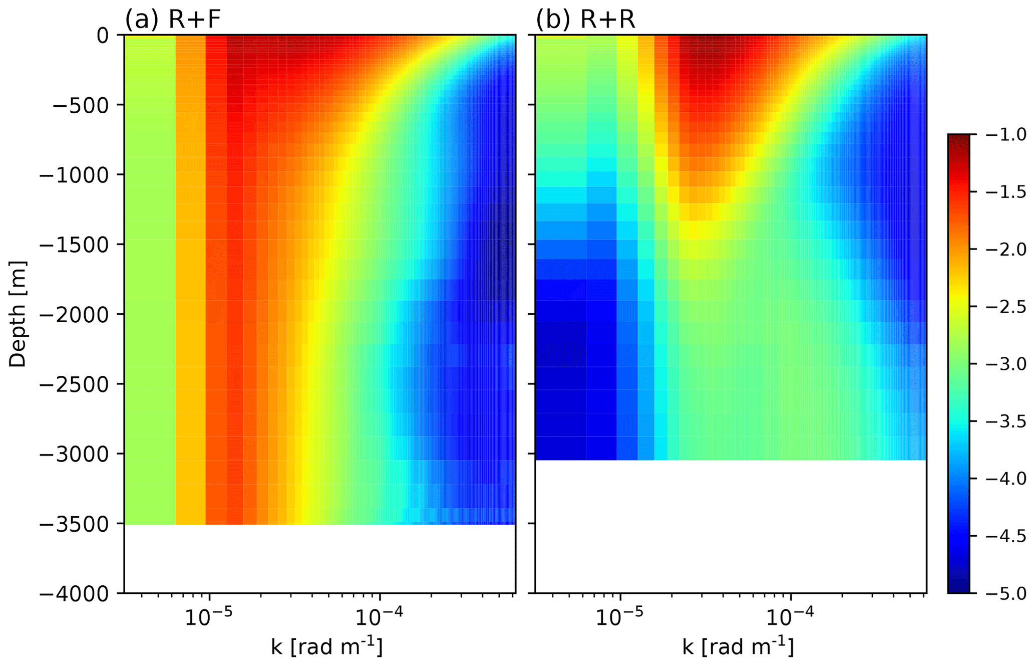
Figure 7Kinetic energy power spectra (log10 m3 s−2) as a function of wavenumber (rad m−1) and depth for simulations R + F and R + R. Spectra are built using instantaneous velocity taken each month of the last 10 years of simulations. Spectra were computed only for depths fully filled by the ocean, outside of the ridge.
3.2.2 Storm track intensity
More locally, dynamics in the lee of the ridge is largely affected by bottom roughness. The comparison between R + F and R + R shows that bottom roughness reduces the zonal extent of the standing meander (Fig. 8a; see also Fig. 3) and the EKE levels in the lee of the ridge (Fig. 8b). This is associated with a weakening of the local baroclinic instability conversion, as revealed by weaker vertical eddy buoyancy flux in R + R in the vicinity of the ridge and meander (Fig. 8c). The response is distinct in the rest of the domain where bottom roughness leaves EKE levels approximately unchanged (Fig. 8b) and even slightly increases EKE along the ACC path (compare Fig. 3b and e).
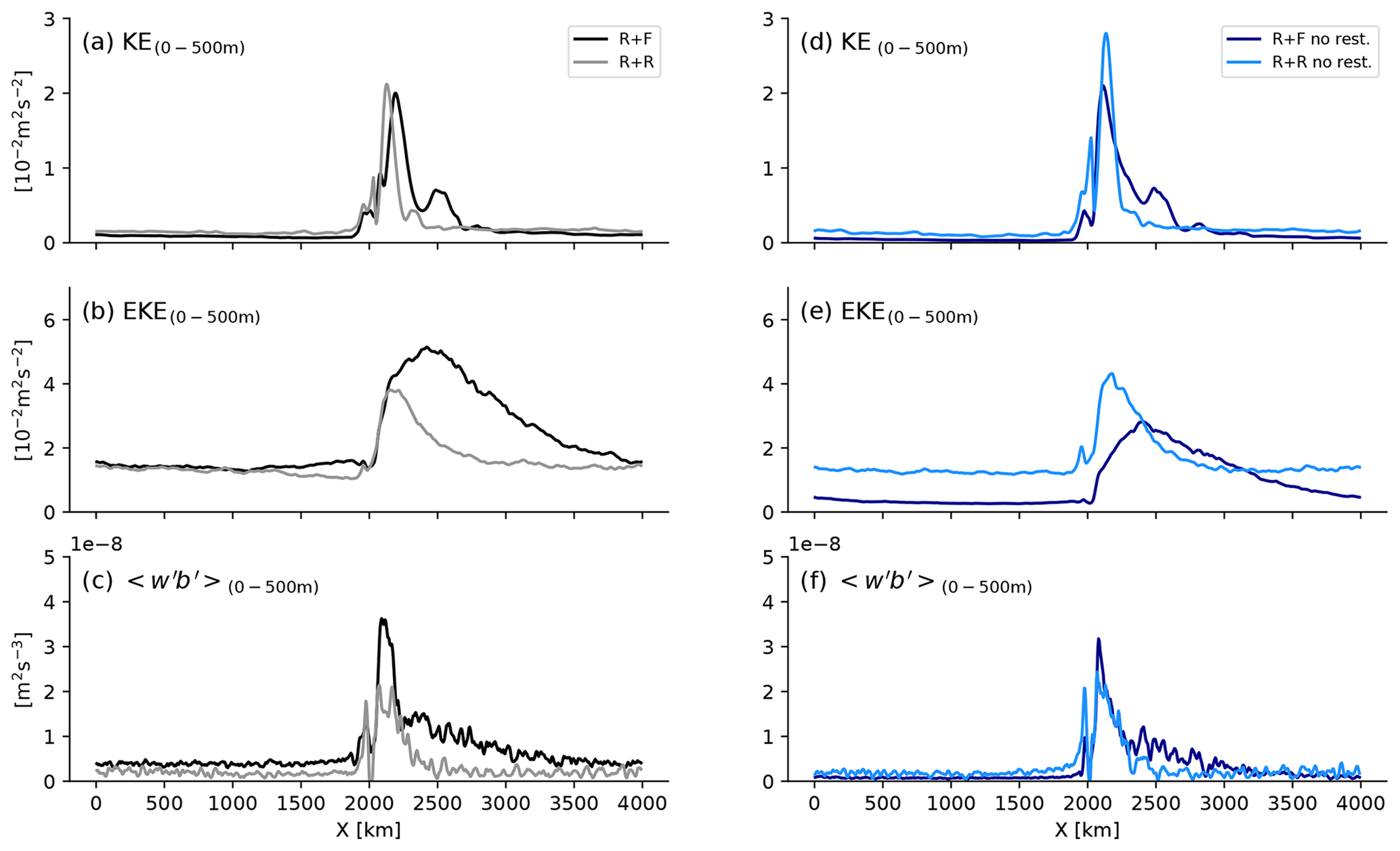
Figure 8Zonal distribution of 10-year-averaged (a, d) mean kinetic energy (m2 s−2), (b, e) eddy kinetic energy (m2 s−2) and (c, f) vertical eddy buoyancy flux (m2 s−3). Quantities were averaged over the full domain in the meridional direction and between the surface and 500 m depth. The velocity (u′, v′, w′) and buoyancy (b′) anomalies use to compute the eddy kinetic energy in (a) and the buoyancy flux in (c) and(f) are anomalies with respect to the 10-year temporal mean.
3.2.3 Strength of the gyre mode
Wind-driven gyres in the lee of tall topographic ridges are a potential attribute of the SO circulation that has received recent attention (Nadeau and Ferrari, 2015; Patmore et al., 2019) but still need to be better understood, including observationally. Essential to making progress is to understand the ACC response to wind stress curl input and balance of vorticity. In R + F the barotropic streamfunction (Fig. 9a) reveals the presence of closed recirculating gyres in the lee of the meridional ridge, consistent with the double-gyre circulation found by Nadeau and Ferrari (2015) in the presence of a tall ridge. When rough topography is added, the southern (resp. northern) gyre completely (resp. nearly) disappears (Fig. 9c and e, where the meridional structure of the zonal flow in the lee of the ridge is represented).
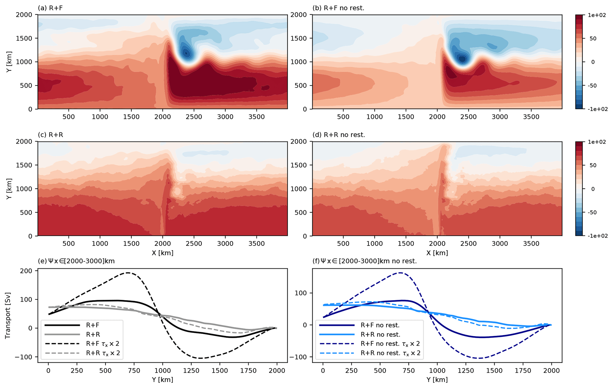
Figure 9Barotropic streamfunction (Sv) for (a) R + F, (b) R + R, (c) R + Fnr and (d) R + Rnr. Transport averaged between x=2000 and 3000 km for the set of reference simulation (bold lines) and simulations with maximum wind stress increased 2-fold, with (e) restoring and (f) without restoring.
To help interpret this result, the barotropic vorticity balance in R + R and R + F averaged between y=400 and 600 km is shown in Fig. 10 for two portions of the zonal domain: an area under direct influence of the ridge (between x=1500 and 2500 km) and an area including the rest of the zonal domain. In the range of latitude considered, the western boundary current forming at the ridge location is northward and well defined in R + F (Fig. 9). This is reflected in the BV balance by the negative and large values of the term −βV (Fig. 10a). At first order, this northward flow is balanced by the bottom pressure torque. In the rest of the domain (Fig. 10b), pressure torque is zero (because the bottom is flat), and the wind stress curl is balanced by a southward barotropic flow. This is the classical wind-driven gyre balance (Munk, 1950; Hughes and De Cuevas, 2001; Nadeau and Ferrari, 2015) whose relevance to the real SO remains uncertain as mentioned above.
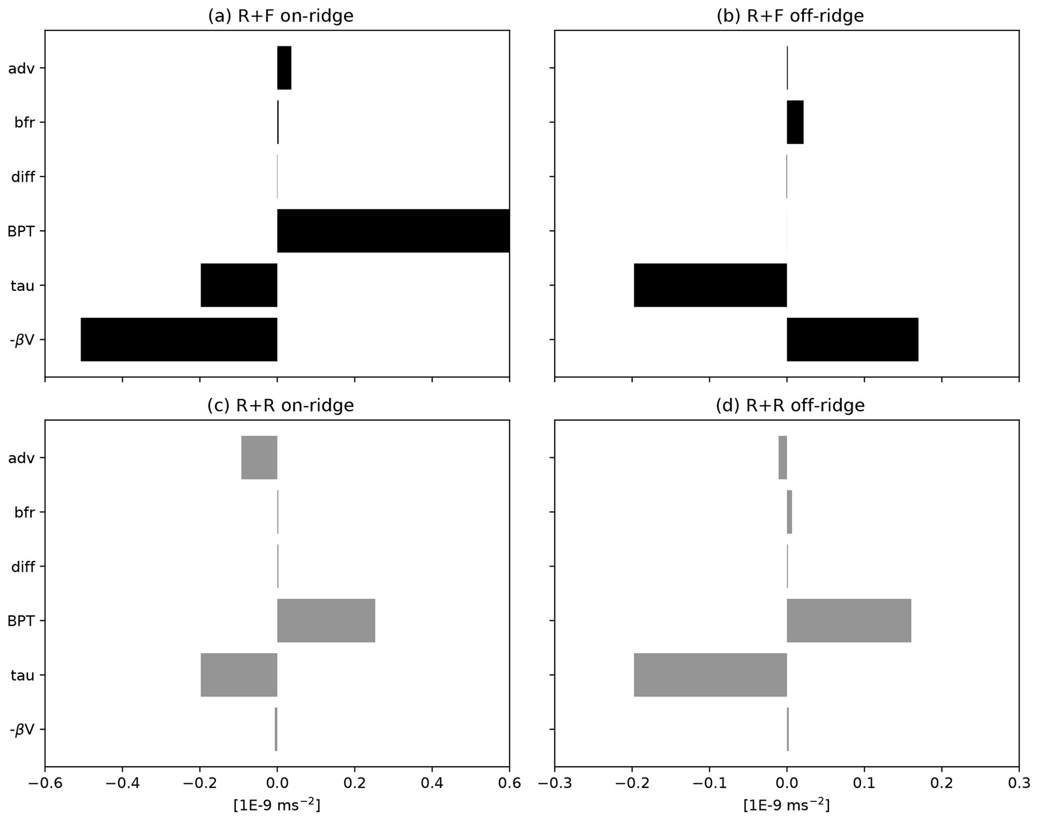
Figure 10Depth-integrated mean barotropic vorticity balance (10−9 m s−2) averaged between y=400 and y=600 km for two zonal portions of the domain: (a, c) one under direct influence of the ridge (between x=1500 and 2500 km) and (b, d) one including the rest of the zonal domain. The different terms are as follows: the advection of planetary vorticity (−βV), the wind stress curl (tau), the bottom stress curl (bfr), the bottom pressure torque (BPT), the diffusion (which includes the effects of the lateral diffusion and Asselin time filter) and the nonlinear advection of vorticity (adv).
The vorticity balance is fundamentally different when rough topography is included. First, the northward barotropic flow at the ridge location present in R + F is absent (Fig. 10c). The bottom pressure torque there mainly acts to balance the local wind stress curl. In the rest of the domain, the vorticity balance is similar to that occurring at the ridge: a large fraction of the wind stress curl is balanced by bottom pressure torque, limiting both the southward transport and the influence of the bottom friction.
3.3 Sensitivity to northern restoring
In R + F and R + R, the joint action of the air–sea heat fluxes and eddy buoyancy fluxes set the interior stratification and large-scale dynamical equilibrium of the ACC. The restoring of the density field toward a specified profile at the northern boundary can be seen as an additional thermohaline constraint that prevents an equilibration of the two solutions in widely different states. We now compare this set of simulations with restoring at the northern boundary (simulations R + F and R + R) to a similar one without the restoring (simulations R + Fnr and R + Rnr). Simulations without restoring may be thought of as idealized representations of an ocean where the SO dynamics dictates hydrographic conditions north of the ACC path to the rest of the world ocean (though with the remaining constraint that the residual overturning circulation be zero). Conversely, simulations with restoring would represent conditions in which the rest of the world ocean imposes a fixed stratification at the northern edge of the SO. Each is a limit case distinct from the real ocean where significant water mass transformation occurs in the SO with large rates of water volume import–export by the meridional overturning cells.
Most of our previous results are not qualitatively dependent on the choice of restoring the northern stratification. Specifically, adding rough bathymetry without northern restoring still does the following: increases the ACC transport (Fig. 5b, e); decreases deep MKE and EKE (Fig. 4a, b); weakens the vertical buoyancy flux in the lee of the ridge (Fig. 8f), although only slightly with no restoring; and strongly affects the BV balance in such a way that wind-driven gyres are present (resp. absent) in smooth (resp. rough) bottom conditions (Fig. 9). Two important distinctions are noteworthy. First, the ACC transport sensitivity is far greater without northern restoring (∼170 % increase from 23 Sv in R + Fnr to 62 Sv in R + Rnr). Second, bottom roughness strongly decreases total KE when restoring is applied, while total KE is very weakly affected when no restoring is applied (Fig. 5a, d). We attribute this to the fact that the more efficient release of available potential energy in the absence of rough bathymetry (Fig. 4c), leading to larger EKE in the upper 500 m (Fig. 4b), can significantly modify the ACC thermohaline structure in the simulations without restoring, whereas it cannot when tightly constrained by the restoring (compare the departures between isotherms in Fig. 5c and f). Further elaboration is provided in Sect. 4.
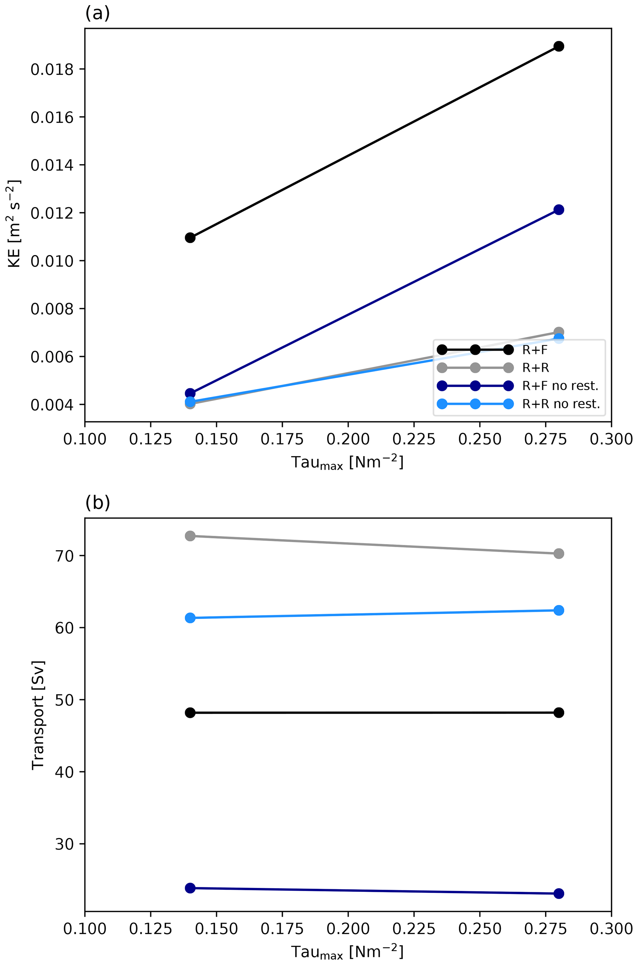
Figure 11Sensitivity of (a) domain-averaged KE (m2 s−2) and (b) zonal barotropic transport (Sv) to wind stress increase. Transport and KE values were averaged for the last 10 years of simulation once equilibrium was achieved.
3.4 Sensibility to wind stress increase
Sensitivity to wind intensity is explored by doubling the wind stress forcing for all simulations previously used. In agreement with the dominant theory (e.g., Meredith and Hogg, 2006; Morrison and Hogg, 2013), all the configurations respond with an increase in the total kinetic energy (Fig. 11a) but exhibit a saturation of the zonal transport (Fig. 11b). In R + F and R + Fnr, the saturation is accompanied by a strengthening of the recirculating gyre (Fig. 9e, f), as observed in Nadeau and Ferrari (2015). In presence of rough topography, the weak gyre circulation previously found in the northern part of the domain intensifies slightly. In the south, close examination of Fig. 9e and f reveals that the barotropic streamfunction develops weak maxima near y=500 km for doubled wind intensity. The tendency to form wind-driven gyres is minor though and occurs while the nature of the BV balance remains unchanged (not shown). Most of the additional wind stress curl is balanced by bottom pressure torque in and out of the ridge area, as opposed to meridional Sverdrup transport. This result questions the recent interpretation of the transport saturation mechanism placing emphasis on the coexistence of a gyre mode together with the circumpolar flow (Nadeau and Ferrari, 2015; see Sect. 4).

Figure 12Times series of zonal transport (Sv) and total kinetic energy (m2 s−2) for simulations R + F (black lines) and R + R (gray lines) in response to an abrupt doubling of the wind stress at year 150. Inset provides details for the years 149–204. The blue dashed (resp. dotted) lines represent the average (resp. average ±1 standard deviation) transport between years 130 and 150.
On the other hand, the transient response to wind increase in the presence and absence of bottom roughness are distinct in important ways. In Fig. 12 we present the time series of circumpolar transport and EKE for R + F and R + R. Insets provide enhanced details for the period where the solutions adjust to the sudden wind intensity doubling at t=150 years. Adjustments were monitored with outputs at monthly frequency, which limits our ability to determine short timescales precisely. More importantly, a difficulty arises from the fact that the temporal changes following the wind increase combine a deterministic response and stochastic variability. A large ensemble of simulations would be needed to disentangle the two components, and we limit ourselves to a qualitative description of the main differences between R + F and R + R. The EKE adjustment in R + R occurs over a time period of ∼4 years and roughly conforms to the descriptions made in Meredith and Hogg (2006). In R + F, the EKE adjustment is comparatively much faster. It is nearly completed after 6 months, except for a small downward trend during 10–20 years that follows a slight initial overshoot.
No transport adjustment is discernible in R + F, and this is in sharp contrast with R + R. An initial transport increase of about 8 Sv occurs over the first few months. The subsequent time period of about 15–20 years exhibits a trend toward smaller transports. Toward year 165, the circumpolar transport has finally returned to steady state with values a few sverdrups below those prior to the wind increase. Note that the initial spinup of R + R also includes a secondary adjustment period between years 60 and 100 (Fig. 5) which is absent in R + F.
The reasons underlying the adjustment differences between R + R and R + F are examined in the context of the saturation theory in Sect. 4.
4.1 Dynamical interpretation of the bottom roughness effect
This part of the discussion is an attempt to hold and connect together (in words) the following: (1) the issue of flow–topography interactions and (2) their consequences (in cascade order) for the barotropic component of the flow, (3) the BV balance, (4) baroclinic instability and the storm track dynamics in the vicinity of the ridge, and finally (5) the ACC transport3.
4.1.1 (1) Flow–topography interactions and (2) barotropic circulation
Starting from (1) we remind the reader that the impact of bottom topography on the general circulation and how it responds to atmospheric forcings has been studied for a long time (e.g., Munk and Palmén, 1951; Tréguier and McWilliams, 1990; Hughes and De Cuevas, 2001; Ward and Hogg, 2011). In our simulations hrms is large enough for the f∕h potential vorticity field to be dominated by numerous closed isolines. In this situation, the barotropic component of the flow is strongly affected (Tréguier and McWilliams, 1990; Hugues and Killworth, 1995; LaCasce, 2010). Specifically, barotropic Rossby waves are no longer permitted (Anderson and Killworth 1977; LaCasce, 2017). In the context of closed basins, wind-driven gyres and a Sverdrup balance are nonetheless being established in the upper ocean by the baroclinic Rossby waves (Anderson and Killworth, 1979). However, this is not possible in the context of the ACC where baroclinic Rossby wave propagation is too slow compared to advection by the mean flow. As a consequence, only in the flat bottom configuration can the Sverdrup balance emerge.
Beside the effect on Rossby wave modes, the barotropic circulation is greatly diminished in the presence of rough bathymetry (Fig. 7) and so is the strength of the deep circulation (Fig. 9). Our interpretation is that the presence of the topography inhibits or counteracts (Trossman et al., 2017) the barotropization process generally associated with turbulent geophysical flows (Salmon et al., 1976). Horizontally integrated energy budgets carried out for different depth layers of fluid provide support to this interpretation4. In R + F, pressure work is a term of dominant importance in the flow energetics. It transfers KE vertically from the upper ocean (0–1500 m depth) into the deep ocean (3000–4000 m depth). The magnitude of the transient KE transfer into the deep layer (computed with buoyancy, pressure and velocity anomalies respective to zonally averaged values) is reduced by a factor over 3.5 in the presence of rough bottom – i.e., the barotropization mechanism is greatly hampered. In turn, the slowdown of the deep circulation has important consequences for the flow–ridge interaction whose ability to produce topographic form stress is severely reduced (compare on-ridge magnitude of the pressure torque for R + F and R + R in Fig. 11).
4.1.2 (3) The BV balance
Overall, the differences in flow–topography interactions and their consequences for the barotropic circulation (turbulent flow and linear Rossby wave mode) yield fundamentally different bottom form stress and BV balances. The distribution of bottom form stress is relatively uniform zonally in solutions with rough bottom. Conversely, large bottom form stresses are confined to the east in the lee of ridges in solutions with a smooth bottom, in conjunction with the presence of intensified boundary currents. The BV balance and boundary currents then resemble those typical of wind-driven gyres (Nadeau and Ferrari, 2015; Fig. 10). Conversely, bottom pressure torque cannot balance wind curl input in R + F away from the ridge where the bottom is flat. Thus, meridional flows develop as part of a Sverdrupian BV balance typical of subpolar and subtropical wind-driven gyres. The boundary current needed to close the circulation and satisfy the continuity equation can only occur about the ridge where nonzero form stress is permitted. Specifically, the boundary current and large bottom pressure torque are found on the eastward side of the ridge, given the direction of propagation of Rossby waves (Nadeau and Ferrari, 2010; Fig. 10). This difference in how the BV balance is satisfied in R + F and in R + R has major implications.
4.1.3 (3) Baroclinic instability and (5) ACC transport sensitivity
The circulation pattern resulting from the interaction between an ACC-like flow and a ridge (the so-called “standing wave response” in Abernathey and Cessi, 2014) is responsible for intense frontogenesis, available potential energy (APE) release and eddy heat fluxes in the lee of the ridge. In the same sector, simulations with a smooth bottom produce boundary currents which combine to the standing wave response and further enhance the frontogenetic tendency and the overall ability of the storm track to release APE, thereby acting to flatten the isopycnals and limit the ACC transport. Note that the distribution of transport is also significantly different because the barotropic mode is so much more energetic with a flat bottom, not only for the gyre circulation but also for the ACC transport mode.
The reduced baroclinicity and zonal transport in R + F and R + Fnr can thus be seen as the manifestation of the boundary current effect on local baroclinic instability in the lee of the ridge. In the simulations without restoring, this manifestation of baroclinic instability is less evident because the mean thermohaline structure of the ACC has significantly more freedom to adjust in response to the strength of baroclinic instability processes. In turn, this response of the mean state leads to a negative feedback by modulating the intensity of baroclinic processes that ends up being quite similar with and without rough bathymetry in the absence of northern restoring (compare EKE and APE release rate for R + Fnr and R + Rnr in Figs. 4c and 8f), relative to what is found with the northern restoring.
Overall, the surprising transport sensitivity that motivated this study reveals important upscaling effects resulting from mesoscale flow–topography interactions. They corroborate the finding of Nadeau et al. (2013) in a quasi-geostrophic framework that the ACC transport increases when the realism of flow–topography interactions is improved. Our work contributes to its interpretation and strives to unravel the underlying causal chain of processes. Our results complement those of Barthel et al. (2017), Constantinou et al. (2019) and Patmore et al. (2019) in drawing attention to the barotropic flow component. Although baroclinic instability is, in our simulations, what ultimately sets the ACC density structure and transport, the barotropic flow plays a key role in modulating the propensity of the eddies to relax baroclinicity.
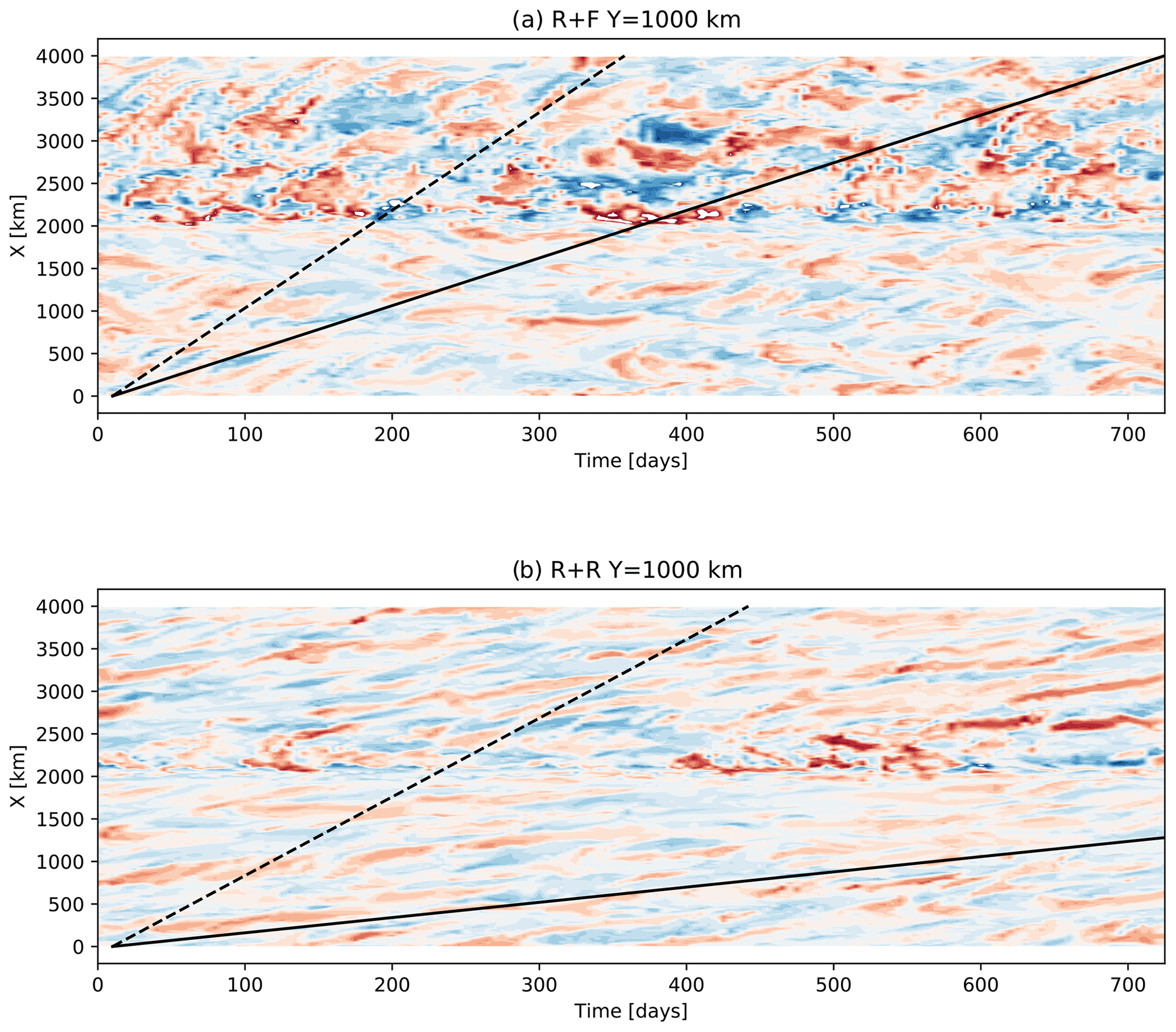
Figure 13Hovmöller diagram of surface temperature anomalies at Y=1000 km as in Abernathey and Cessi (2014) built using 5 d averaged model outputs for a 2-year period. The dashed line indicates the zonal surface velocity and the continuous line indicates the barotropic velocity
The beginning of this research developed with the hypothesis that R + F and R + R differed in the characteristics of their dominant mode of baroclinic instability and a stronger (resp. weaker) local instability mode in R + F (resp. R + R). Here, local instability mode refers to the definition proposed by Pierrehumbert (1984). The concept of local instability mode is used by Abernathey and Cessi (2014) to rationalize the behavior of a simulation resembling R + F. The onset of gyres and associated boundary currents when the ocean floor is smooth certainly makes local baroclinic instability modes growing in the vicinity of the ridge stronger. Given the specifics of local instability developments we might thus expect to see a lesser tendency for flow perturbations in R + R to remain quasistationary in the vicinity of the ridge (Pierrehumbert, 1984; Abernathey and Cessi, 2014). Hovmöller diagrams for surface temperature perturbations in R + R and R + F show no particular evidence of this (Fig. 13). Also note that R + R has lower baroclinic conversion rates than R + F not only about the ridge but also far outside its range of influence. A simple and general dynamical explanation for the baroclinic instability sensitivity to bottom roughness revealed in this study would be that rough topography upsets the subtle coupling between fluid layers required for baroclinic instability perturbations to grow by constraining the mean and time-variable flow.
4.2 Implications for the eddy saturation process
Baroclinic instability, which is the main source of energy for the mesoscale eddy field in the SO consumes the APE imparted by wind-driven upwelling. It occurs in such a way that additional energy input by the wind enhances EKE but leaves APE and ACC transport nearly unchanged. This contributes to the so-called eddy saturation effect which limits the sensitivity of the circumpolar transport to changes in the wind forcing magnitude (Morrison and Hogg, 2013; Munday et al., 2013; Marshall et al., 2017). Processes involving the barotropic circulation and its interaction with the bathymetry may also participate in reducing the sensitivity of the ACC's baroclinicity. The analysis of the energetics of an ACC standing meander in Youngs et al. (2017) reveals that barotropic instability plays a leading role in the energy budget of the meander and suggests that baroclinic conversion alone is insufficient to describe both the stratification and distribution of EKE. The standing meanders that form through the interaction of the barotropic flow with the topography contribute to the bottom form stress and may also participate in the saturation process (Thompson and Naveira Garabato, 2014; Katsumata, 2017). Constantinou and Hogg (2019) recently highlighted the role played by the eddy production through lateral shear instabilities of the barotropic circulation or interaction of the barotropic current with the topography, in establishing the eddy saturated state of the Southern Ocean. Overall, our findings confirm the robustness of the saturation process with respect to major changes in model configuration, which translate into a wide range of baroclinic instability regimes and efficiency (as previously noted in Nadeau et al., 2013), mean flow with widely distinct barotropic characteristics and ACC transports. In particular, the saturation process is more generic than the study by Nadeau and Ferrari (2015) suggests. The work of Nadeau and Ferrari (2015) highlights the role of the gyre mode and Sverdrup balance in the saturation mechanism. To the contrary, in our study the effectiveness of the saturation process (e.g., measured as the long-term relative change in ACC transport when doubling the wind intensity) is insensitive to the presence or absence of a wind-driven gyre component in the SO.
In Nadeau and Ferrari (2015), increasing the bottom drag coefficient reduces the intensity of the gyre circulation and also impedes the ACC transport saturation. A similar sensitivity of the transport saturation to bottom drag is also observed by Marshall et al. (2017). Bottom roughness and bottom drag are sometimes thought to be interchangeable ways to boost the topographic control over oceanic flows (Arbic and Flierl, 2004; LaCasce, 2017). As anticipated by Nadeau and Ferrari (2015), this is not the case with respect to the saturation process whose efficiency is not affected by bottom roughness, whereas increased bottom drag reduces the intensity of the gyre circulation and also impedes the ACC transport saturation. We attribute this to the fact that large bottom drag produces a nonphysical damping of the turbulent flow and changes the nature of the momentum and vorticity balances – we recall that bottom form stress is not a drag force (Tréguier and McWilliams, 1990) and, in particular, provides no sink in the energy budget.
Recently, Sinha and Abernathey (2016) have offered important insight into the transient behavior of an ACC system subjected to wind changes. Following wind intensification, saturation is the final outcome of a process involving two stages: a rapid buildup of APE (and ACC transport increase), followed by a slower buildup of EKE which feeds back onto baroclinic instability efficiency (Marshall et al., 2017) and allows APE (and ACC transport) to return back to (or near) their initial levels. Timescales needed for saturation to act on R + F and R + R turn out to be markedly different. Most interestingly, R + F has an almost immediate equilibration of EKE levels to wind changes, and no transient effect on ACC transport can be noticed at the monthly temporal resolution we used to track simulation spinups. The response time of R + R is on the order of a few years, in line with typical values reported by previous studies. Following up on the dynamical discussion in Sect. 4a, we interpret the rapid adjustment in R + F described in Sect. 3 as follows: barotropic Rossby waves with phase speeds of a few meters per second (m s−1) adjust the interior Sverdrup transport to new wind conditions in about 10 d (i.e., the timescale to travel across the entire domain); adjustment of the compensating boundary transport on the eastern side of the ridge follows a somewhat slower but comparable pace (Anderson and Gill, 1975); density advection by the boundary current locally modifies frontogenetic conditions on timescales of weeks (advection is slower than barotropic Rossby wave propagation, but meridional distances to be covered by advection are smaller than the zonal scale of the system); EKE responds on timescales of ∼ weeks typical of baroclinic instability growth (Tulloch et al., 2011) and locally provides the additional APE release and lateral heat fluxes necessary to prevent APE and circumpolar transport to increase. In R + R, barotropic Rossby waves are not permitted, and a much slower baroclinic adjustment process of diffusive nature unfolds as described in Sinha and Abernathey (2016). The response of EKE in R + F is faster than typically estimated in many observational (Meredith and Hogg, 2006; Morrow et al., 2010) or realistic modeling studies (Meredith and Hogg, 2006; Langlais et al., 2015) but this remains a subject of debate (Wilson et al., 2014). Recent numerical experiments (Patara et al., 2016) indicate that the correlation between wind and EKE underlying the eddy saturation mechanism are sensitive to the regional level of bottom roughness. In this context, we hypothesize that the main topographic obstacles in the SO delimit a small number of sectors whose dynamics includes a degree of gyre circulation that depends on the small-scale/mesoscale bathymetry. More specifically, the spatial extension and shape of the main gyres, the Ross and Weddell gyres, could in part be constrained by topographic roughness. Realistic SO simulations that differ in their bottom roughness would be instructive to examine this hypothesis.
The comparison between different numerical simulations for a re-entrant zonal jet revealed that the baroclinicity of the flow is sensitive to current–topography interactions in the mesoscale range 10–100 km, with large consequences for the zonal and gyre transport.
Using semi-realistic simulations of the SO, this study investigates the influence of bottom roughness on the dynamics of an idealized ACC-type flow. While relying on a limited number of simulations, our analyses offer important insight into the sensitivities of ACC model representations. A key ingredient impacting the ACC dynamics is the presence of tall obstacles that provide support for form stress and bottom pressure torque. The main sensitivity explored herein concerns more complex flow–topography interactions and more specifically the role of “random” rough bathymetry combined with a tall ridge. Bottom roughness (with a hrms of 250 m, typical of abyssal hills) is found to have profound consequences for the ACC equilibration. Specifically, it damps the barotropic mode, which has major implications on the momentum and barotropic vorticity balances. In turn, this affects the efficiency of baroclinic instability processes at releasing APE and limit the circumpolar transport. The role of the ACC barotropic component is a subject of active research and our work complements the recent studies of Patmore et al. (2019) and Constantinou et al. (2019) in this regard.
Overall, our study points to the importance and sensitivity of current–topography interactions in the mesoscale range (10–100 km) for the dynamics of the ACC. The question of whether the real ocean is in a regime that is more aptly described by our rough or smooth simulation remains to be elucidated. From a modeling perspective, the bottom roughness considered in this study enters in a scale range of bottom topography which is unequally resolved by climate or global circulation models at a resolution between 1∕4 and 1∘. Recent efforts have been dedicated to parameterizing energy dissipation and mixing caused by the abyssal hills (Nikurashin et al., 2010b; De Lavergne et al., 2016). To our knowledge the impact of subgrid-scale topographic drag has, on the other hand, been forsaken in ocean modeling. Our results advocate for a systematic and scale-dependent exploration of flow–topography interactions so that the transfer of momentum due to bottom form stress is realistically represented irrespective of the unresolved bottom roughness. A starting point is available in atmospheric sciences where approaches have been developed to parameterize subgrid-scale orographic drag (e.g., Lott and Miller, 1997).
Model results can be reproduced by using the ocean code nemo_v3_6 (http://forge.ipsl.jussieu.fr/40nemo/ wiki/Users, last access: 11 December 2017, Madec et al., 2014).
JJ and XC both designed the research study, conducted the analysis and wrote the manuscript. JJ performed the numerical simulations.
The authors declare that they have no conflict of interest.
Supercomputing facilities were provided by GENCI projects GEN7298 and GEN1140. A special thanks to Jérome Chanut for discussion and his assistance with the model setup. We are grateful to the two anonymous reviewers for their insightful comments that helped improve the paper.
This study has been supported by IRD and CNRS and has been funded by the French ANR project SMOC (grant ANR-11-JS56-0009).
This paper was edited by Neil Wells and reviewed by two anonymous referees.
Abernathey, R. and Cessi, P.: Topographic enhancement of eddy efficiency in baroclinic equilibration, J. Phys. Oceanogr., 44, 2107–2126, 2014.
Abernathey, R., Marshall, J., and Ferreira, D.: The Dependence of Southern Ocean Meridional Overturning on Wind Stress, J. Phys. Oceanogr., 41, 2261–2278, 2011.
Anderson, D. L. T. and Gill, A. E.: Spin-up of a stratified ocean, with applications to upwelling, Deep-Sea Res., 22, 583–596, 1975.
Anderson, D. L. T., and Killworth, P. D.: Spin‐up of a stratified ocean, with topography, Deep Sea Res., 24, 709–732, 1977.
Arbic, B. K. and Flierl, G. R.: Baroclinically unstable geostrophic turbulence in the limits of strong and weak bottom Ekman friction: Application to midocean eddies, J. Phys. Oceanogr., 34, 2257–2273, 2004.
Barthel, A., Hogg, A. McC., Waterman, S., and Keating, S.: Jet-topography interactions affect energy pathways to the deep Southern Ocean, J. Phys. Oceanogr., 47, 1799–1816, https://doi.org/10.1175/JPO-D-16-0220.1, 2017.
Barnier, B., Siefridt, L., and Marchesiello, P.: Thermal forcing for a global ocean circulation model using a three-year climatology of ECMWF analyses, J. Mar. Syst., 6, 363–380, 1995.
Bischoff, T. and Thompson, A. F.: Configuration of a Southern Ocean storm track, J. Phys. Oceanogr., 44, 3072–3078, 2014.
Chapman, C. C., Hogg, A. M. , Kiss, A. E., and Rintoul, S. R.: The dynamics of Southern Ocean storm tracks, J. Phys. Oceanogr., 45, 884–903, 2015.
Constantinou, N. C. and Hogg, A. M.: Eddy saturation of the Southern Ocean: a baroclinic versus barotropic perspective, Geophys. Res. Lett., 46, 12202–12212, 2019.
De Lavergne, C., Madec, G., Le Sommer, J., Nurser, A. G., and Naveira Garabato, A. C.: The impact of a variable mixing efficiency on the abyssal overturning, J. Phys. Oceanogr., 46, 663–681, 2016.
Gille, S. T.: The Southern Ocean momentum balance: Evidence for topographic effects from numerical model output and altimeter data, J. Phys. Oceanogr., 27, 2219–2232, 1997.
Goff, J. A.: Global prediction of abyssal hill root-mean-square heights from small-scale altimetric gravity variability, J. Geophys. Res., 115, B12104, https://doi.org/10.1029/2010JB007867, 2010.
Goff, J. A. and Arbic, B. K.: Global prediction of abyssal hill roughness statistics for use in ocean models from digital maps of paleo-spreading rate, paleo-ridge orientation, and sediment thickness, Ocean Modell., 32, 36–43, 2010.
Goff, J. A. and Jordan, T. H.: Stochastic modeling of seafloor morphology: Inversion of sea-beam data for second-order statistics, J. Geophys. Res., 93, 13589–13608, 1988.
Hughes, C. W.: Nonlinear vorticity balance of the Antarctic Circumpolar Current, J. Geophys. Res.-Oceans, 110, C11008, https://doi.org/10.1029/2004JC002753, 2005.
Hughes, C. W. and Killworth, P. D.: Effects of bottom topography in the large‐scale circulation of the Southern Ocean, J. Phys. Oceanogr., 25, 2485–2497, 1995.
Hughes, C. W. and De Cuevas, B. A.: Why western boundary currents in realistic oceans are inviscid: A link between form stress and bottom pressure torques, J. Phys. Oceanogr., 31, 2871–2885, 2001.
Jackson, L., Hughes, C. W., and Williams, R. G.: Topographic control of basin and channel flows: The role of bottom pressure torques and friction, J. Phys. Oceanogr., 36, 1786–1805, 2006.
Jouanno, J., Capet, X., Madec, G., Roullet, G., and Klein, P.: Dissipation of the energy imparted by mid-latitude storms in the Southern Ocean, Ocean Sci., 12, 743–769, 2016.
Karsten, R. H. and Marshall, J.: Testing theories of the vertical stratification of the ACC against observations, Dyn. Atmos. Oceans, 36, 233–246, 2002.
Katsumata, K.: Eddies observed by Argo floats. Part II: Form stress and streamline length in the Southern Ocean, J. Phys. Oceanogr., 47, 2237–2250, https://doi.org/10.1175/JPO-D-17-0072.1, 2017.
LaCasce, J. H.: The prevalence of oceanic surface modes, Geophys. Res. Lett., 44, 11–97, 2017.
LaCasce, J. H. and Isachsen, P. E.: The linear models of the ACC, Prog. Oceanogr., 84, 139–157, 2010.
Large, W. G. and Yeager, S.: The global climatology of an interannually varying air-sea flux data set, Clim. Dynam., 33, 341–364, https://doi.org/10.1007/s00382-008-0441-3, 2009.
Langlais, C. E., Rintoul, S. R., and Zika, J. D.: Sensitivity of Antarctic Circumpolar Current transport and eddy activity to wind patterns in the Southern Ocean, J. Phys. Oceanogr., 45, 1051–1067, 2015.
Lott, F. and Miller, M. J.: A new subgrid-scale orographic drag parametrization: Its formulation and testing, Q. J. Roy. Meteor. Soc., 123, 101–127, 1997.
Madec, G.: “NEMO ocean engine” (Draft edition r5171), Note du Pôle de modélisation, Institut Pierre-Simon Laplace (IPSL), France, No 27 ISSN 1288-1619, 2014.
Marshall, D. P., Ambaum, M. H., Maddison, J. R., Munday, D. R., and Novak, L.: Eddy saturation and frictional control of the Antarctic Circumpolar Current, Geophys. Res. Lett., 44, 286-292, 2017.
Masich, J., Chereskin, T. K., and Mazloff, M. R.: Topographic form stress in the Southern Ocean state estimate, J. Geophys. Res.-Oceans, 120, 7919–7933, 2015.
Meredith, M. P. and Hogg, A. M.: Circumpolar response of Southern Ocean eddy activity to a change in the Southern Annular Mode, Geophys. Res. Lett., 33, L16608, https://doi.org/10.1029/2006GL026499, 2006.
Morrison, A. K. and Hogg, A. M.: On the relationship between Southern Ocean overturning and ACC transport, J. Phys. Oceanogr., 43, 140–148, 2013.
Morrow, R., Ward, M. L., Hogg, A. M., and Pasquet, S.: Eddy response to Southern Ocean climate modes, J. Geophys. Res.-Oceans, 115, C10030, https://doi.org/10.1029/2009JC005894, 2010.
Munday, D., Johnson, H., and Marshall, D.: Eddy saturation of equilibrated circumpolar currents, J. Phys. Oceanogr., 43, 507–532, https://doi.org/10.1175/JPO-D-12-095.1, 2013.
Munday, D. R., Johnson, H. L., and Marshall, D. P.: The role of ocean gateways in the dynamics and sensitivity to wind stress of the early Antarctic Circumpolar Current, Paleoceanography, 30, 284–302, https://doi.org/10.1002/2014PA002675, 2015.
Munk, W. H.: On the wind-driven ocean circulation, Journal of Meteorology, 7, 80–93, 1950.
Munk, W. H. and Palmén, E.: Note on the dynamics of the Antarctic Circumpolar Current, Tellus, 3, 53–55, 1951.
Nadeau, L. P. and Ferrari, R.: The role of closed gyres in setting the zonal transport of the Antarctic Circumpolar Current, J. Phys. Oceanogr., 45, 1491–1509, 2015.
Nadeau, L. P., Straub, D. N., and Holland, D. M.: Comparing idealized and complex topographies in quasigeostrophic simulations of an antarctic circumpolar current, J. Phys. Oceanogr., 43, 1821–1837, 2013.
Naveira Garabato, A. C., Nurser, A. G., Scott, R. B., and Goff, J. A.: The impact of small-scale topography on the dynamical balance of the ocean, J. Phys. Oceanogr., 43, 647–668, 2013.
Nikurashin, M. and Ferrari, R.: Radiation and dissipation of internal waves generated by geostrophic motions impinging on small-scale topography: Theory, J. Phys. Oceanogr., 40, 1055–1074, 2010a.
Nikurashin, M. and Ferrari, R.: Radiation and dissipation of internal waves generated by geostrophic motions impinging on small-scale topography: Application to the Southern Ocean, J. Phys. Oceanogr., 40, 2025–2042, 2010b.
Nikurashin, M. and Ferrari, R.: Global energy conversion rate from geostrophic flows into internal lee waves in the deep ocean, Geophys. Res. Lett., 38, L08610, https://doi.org/10.1029/2011GL046576, 2011.
Patara, L., Böning, C. W., and Biastoch, A.: Variability and trends in Southern Ocean eddy activity in 1/12 ocean model simulations, Geophys. Res. Lett., 43, 4517–4523, 2016.
Patmore, R. D., Holland, P. R., Munday, D. R., Naveira Garabato, A. C., Stevens, D. P., and Meredith, M. P.: Topographic Control of Southern Ocean Gyres and the Antarctic Circumpolar Current: A Barotropic Perspective, J. Phys. Oceanogr., 49, 3221–3244, 2019.
Pierrehumbert, R. T.: Local and global baroclinic instability of zonally varying flow, J. Atmos. Sci., 41, 2141–2162, 1984.
Reffray, G., Bourdalle-Badie, R., and Calone, C.: Modelling turbulent vertical mixing sensitivity using a 1-D version of NEMO, Geosci. Model Dev., 8, 69–86, https://doi.org/10.5194/gmd-8-69-2015, 2015.
Roullet, G. and Madec, G.: Salt conservation, free surface, and varying levels: a new formulation for ocean general circulation models, J. Geophys. Res.-Oceans, 105, 23927–23942, 2000.
Sallée, J. B., Speer, K., Rintoul, S., and Wijffels, S.: Southern Ocean thermocline ventilation, J. Phys. Oceanogr., 40, 509–529, 2010.
Salmon, R., Holloway, G., and Hendershott, M. C.: The equilibrium statistical mechanics of simple quasi-geostrophic models, J. Fluid Mech., 75, 691–703, 1976.
Sinha, A. and Abernathey, R. P.: Time scales of Southern Ocean eddy equilibration, J. Phys. Oceanogr., 46, 2785–2805, 2016.
Tansley, C. E. and Marshall, D. P.: On the dynamics of wind-driven circumpolar currents, J. Phys. Oceanogr., 31, 3258–3273, 2001.
Thompson, A. F. and Naveira Garabato, A. C.: Equilibration of the Antarctic Circumpolar Current by standing meanders, J. Phys. Oceanogr., 44, 1811–1828, 2014.
Tréguier, A. M. and McWilliams, J. C.: Topographic influences on wind-driven, stratified flow in a β-plane channel: An idealized model for the Antarctic Circumpolar Current, J. Phys. Oceanogr., 20, 321–343, 1990.
Tulloch, R., Marshall, J., Hill, C., and Smith, K. S.: Scales, growth rates, and spectral fluxes of baroclinic instability in the ocean, J. Phys. Oceanogr., 41, 1057–1076, 2011.
Trossman, D. S., Arbic, B. K., Straub, D. N., Richman, J. G., Chassignet, E. P., Wallcraft, A. J., and Xu, X.: The role of rough topography in mediating impacts of bottom drag in eddying ocean circulation models, J. Phys. Oceanogr., 47, 1941–1959, 2017.
Youngs, M. K., Thompson, A. F., Lazar, A. and Richards, K. J.: ACC meanders, energy transfer and mixed barotropic-baroclinic instability, J. Phys. Oceanogr., 47, 1291–1305, https://doi.org/10.1175/JPO--D--16--0160.1, 2017.
Ward, M. and Hogg, A. M.: Establishment of momentum balance by form stress in a wind-driven channel, Ocean Modell., 40, 133–146, https://doi.org/10.1016/j.ocemod.2011.08.004, 2011.
Wilson, C., Hughes, C. W., and Blundell, J. R.: Forced and intrinsic variability in the response to increased wind stress of an idealized Southern Ocean, J. Geophys. Res.-Oceans, 120, 113–130, https://doi.org/10.1002/2014JC010315, 2014.
Wu, L., Jing, Z., Riser, S., and Visbeck, M.: Seasonal and spatial variations of Southern Ocean diapycnal mixing from Argo profiling floats, Nat. Geosci., 4, 363–366, 2011.
Abyssal hills frequently have a length–width aspect ratio of 5 or more (e.g. Goff and Arbic, 2010).
The total KE and the transport take more time to equilibrate in R + R than in R + F (Fig. 5a), with a large KE increase in the first 10 years of spinup and a KE decrease in the following ∼90 years. This slow decrease in the domain-averaged kinetic energy in R + R between years 10 and 100 is related to a slow destratification of the southernmost part of the domain (the weak stratification of the final state can be seen in Fig. 5c). As indicated in Sect. 2, the simulation is initialized using a stratified density profile. During the first years of the simulation there is enough background stratification to sustain the existence of baroclinic eddies over the entire domain. The subsequent uplifting of the isopycnal and associated destratification in the south progressively prevents the existence of baroclinic eddies, while barotropic eddies cannot develop due to the strong constraint exerted by the bottom form stress. At equilibrium, the region located between Y=0 and ∼500 km is devoid of eddies. The time taken for this sequence to unfold may explain the slower transport equilibration in this simulation.
In search for an alternative and possibly simpler interpretation, one reviewer suggested that the transport sensitivities revealed by this study may be the consequence of vertical stratification differences between our simulations (in our primitive equation framework the stratification cannot be held fixed unless artificial restoring is employed). Everything else being unchanged the ACC transport tends to increase with stratification (e.g., in the quasi-geostrophic simulations of Nadeau and Ferrari, 2015). In contrast, we find that stratification is generally stronger in R + F (resp. R + Fnr) than in R + R (resp. R + Rnr). For instance, the stratification averaged over the subdomain 500 km < y<1500 km (the central part of the domain where the zonal flow is intensified) and −3000 m < z<0 (the part of the water column above the topographic hills) is ∼15 % stronger in R + F than in R + R. Thus, the stratification differences cannot be invoked to explain that larger transport values found in R + R than in R + F.
A different interpretation may be proposed in the context of surface mode decomposition (LaCasce, 2017). Surface mode decomposition explicitly accounts for the presence of variable bathymetry in the vertical mode decomposition, which suppresses the barotropic mode.