the Creative Commons Attribution 4.0 License.
the Creative Commons Attribution 4.0 License.
 | 12 Apr 2019
A simple predictive model for the eddy propagation trajectory in the northern South China Sea
Jiaxun Li
Guihua Wang
Huijie Xue
Huizan Wang
A novel predictive model was built for eddy propagation trajectory using the multiple linear regression method. This simple model relates various oceanic parameters to eddy propagation position changes in the northern South China Sea (NSCS). These oceanic parameters mainly represent the effects of β and mean flow advection on the eddy propagation. The performance of the proposed model has been examined in the NSCS based on five years of satellite altimeter data and demonstrates its significant forecasting skills over a 4-week forecast window compared to the traditional persistence method. It was also found that the model forecasting accuracy is sensitive to eddy polarity and the forecast season.
- Article
(4798 KB) - Full-text XML
- BibTeX
- EndNote


Mesoscale eddies are coherent rotating structures that are ubiquitous over most of the world's oceans (Chelton et al., 2007). They play an important role in the transport of momentum, heat, mass, and chemical and biological tracers; thereby they become critical for issues such as general circulation, water mass distribution, ocean biology, and climate change (Wang et al., 2012; Dong et al., 2014; Zhang et al., 2014; Ma et al., 2016; Li et al., 2017). Therefore, forecasting the eddy propagation positions accurately is not only important scientifically, but also important practically for problems such as designing ocean observing systems, fishing planning, and detecting underwater acoustics.
Traditionally, ocean dynamical models were used as a tool to predict the evolution of ocean eddies (Robinson et al., 1984). Since mesoscale eddies are often associated with strong nonlinear processes and their dynamical mechanisms are quite different, the operational forecasting of eddies has been a big challenge for ocean numerical models. Much progress has been made in recent years in eddy-resolving ocean prediction. With data assimilation and the increase of model resolution, model forecasting skills are increasing. Daily forecasting errors of eddy center positions in the northwestern Arabian Sea and the Gulf of Oman are 44–68 km with the 1∕12∘ global HYCOM model and reach to 22.5–37 km with the 1∕32∘ NLOM model (Hurlburt et al., 2008). The forecasting skill and predictability of dynamical models can only be increased by better assimilation schemes (initialization), sufficient data (especially the subsurface), and improving resolution (physics and computing) (Rienecker et al., 1987; Oey et al., 2005). These restrictions preclude the all-pervading operational use of dynamical models when the initial data and computing power are not feasible due to certain reasons.
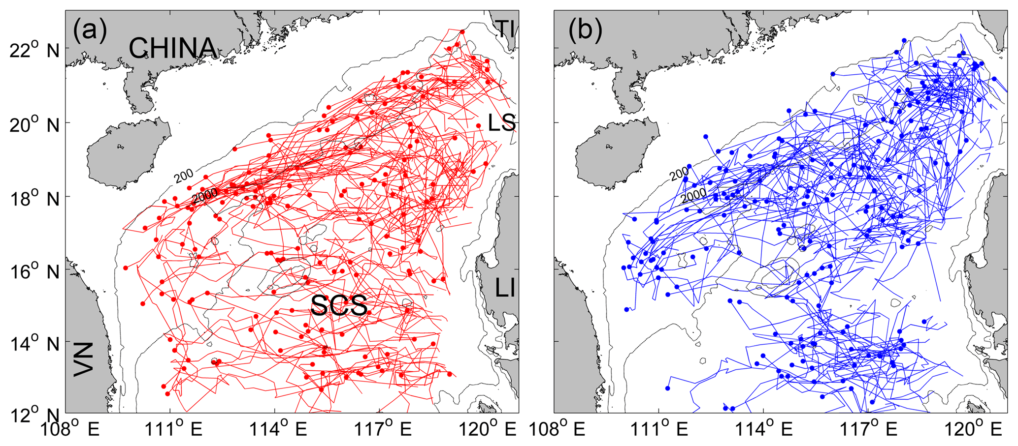
Figure 1The trajectories of (a) anticyclonic and (b) cyclonic eddies with lifetime ≥5 weeks in the northern South China Sea (NSCS). The solid circle represents the ending position of each trajectory. In (a), TI: Taiwan Island, LI: Luzon Island, LS: Luzon Strait, VN: Vietnam. The two isobaths are for 200 and 2000 m, respectively.
In this paper, we developed a simple statistical model to predict the eddy positions 1–4 weeks in advance using only the past positions of the eddy and its surrounding fields. Our “test block” of ocean is the northern South China Sea (NSCS). The South China Sea is a semi-enclosed sea under the dramatic influence of the East Asian monsoon and Kuroshio intrusion (Liu and Xie, 1999; Shaw, 1991). Due to the variable external forcing and complex topography, mesoscale eddies show obvious geographic distributions and various characteristics (Wang et al., 2003; Xiu et al., 2010; Chen et al., 2011). A common characteristic is the overall westward tendency of eddy trajectories regardless of the eddy polarity (Fig. 1). We will first analyze the pattern and dynamics of the common westward movement of eddies in the NSCS, then choose the potential predictors and develop a simple predictive model for eddy propagation trajectories, and finally evaluate the model performance and discuss the impact of eddy polarity and season on the forecasting accuracy.
2.1 Data
The sea level anomalies (SLAs) are from the Archiving, Validation and Interpretation of Satellite Oceanographic data (AVISO; ftp://ftp.aviso.oceanobs.com/, last access: 20 November 2018) (Ducet et al., 2000). AVISO merges the measurements of TOPEX/Poseidon, the European Remote Sensing satellites (ERS-1 and ERS-2), the Geosat Follow-on, Jason-1 and Jason-2 satellites and the Envisat, and spans the period from 14 October 1992 to 7 August 2013. Its temporal resolution is weekly, and its spatial resolution is 0.25∘ latitude by 0.25∘ longitude. To estimate the large-scale geostrophic currents, we use the absolute dynamic topography (ADT), which consists of the SLAs and a mean dynamic topography (MDT). The method for calculating the MDT was introduced by Rio and Hernandez (2004), and the data are also distributed by AVISO.
The monthly climatology of observed ocean temperature and salinity from US Navy's Generalized Digital Environment Model (GDEM-Version 3.0) is used to calculate the phase speed of nondispersive baroclinic Rossby waves in the NSCS. It has a horizontal resolution of 0.25∘ latitude by 0.25∘ longitude, and 78 standard depth layers from 0 to 6600 m with the vertical resolution varying from 2 m at the surface to 200 m below 1600 m (Canes, 2009).
The NSCS eddy trajectory data are derived from the third release of the global eddy dataset (http://cioss.coas.oregonstate.edu/eddies/, last access: 30 March 2017). The eddy center positions within their trajectories are recorded at 7-day time intervals. A detailed description of the eddy trajectory dataset can be found in Chelton et al. (2011). To forecast the eddy trajectory 1–4 weeks in advance using the last position of the eddy, only eddies with a lifetime of 5 weeks or longer are retained in this study.
2.2 The maximum cross-correlation method
The maximum cross-correlation (MCC) method is a space–time-lagged technique, which can estimate the surface motions from time-sequential remote sensing images. It has been successfully used to track clouds from geosynchronous satellite data (Leese et al., 1971), to compute sea-ice motion (Ninnis et al., 1986) and advective surface velocities (Emery et al., 1986) from sequential infrared satellite images, and to determine the propagation velocities of ocean eddies from satellite altimeter data (Fu, 2006, 2009). The MCC method used in this study is the same as that of Fu (2009), which is a little different from that of Emery et al. (1986). In the method of Emery et al., a subarea called the “template window” of the first image is correlated with many identically sized subimages within a large “search window” area of the second image and the speed and direction of the maximum correlation can be estimated. In the method of Fu (2009), the correlations of the SLA at a given location with all the neighboring SLAs at various time lags are computed, and the speed and direction of the maximum correlation can be estimated. The reason for this difference may be due to the low space–time resolution of the SLA compared to other infrared satellite images.
The MCC method mainly consists of two procedures (Fu, 2009). First, the cross-correlations of the SLA time series (h) with others within a certain range box are computed for some time lags (ΔT) in multiples of 7 days (time resolution of SLA data) at each grid node location (x,y) as follows:
where Δx and Δy are the spatial lags and the over bar means time averaging. Second, the position of the maximum correlation at each time lag (ΔT) is identified, and a speed can be derived from the time lag and the distance of this position from the origin calculated. Then an average speed vector (u,v) weighted by the correlation coefficients is calculated from the estimates at various time lags as follows:
where Ci is the maximum correlation at ΔTi, and Δxi, Δyi are the distances between the position of maximum correlation and the origin. The average velocities are then assigned to the eddy movement velocities at the given grid point.
To focus on the global mesoscale eddy, the time lags were limited to less than 70 days and the dimension of the window was less than 400 km (Fu, 2009). In the NSCS, the time lags should be limited to less than 42 days, since with larger time lags many correlation coefficients are below the 95 % confidence level (Zhuang et al., 2010). Besides, Chen et al. (2011) found that eddies propagate with 5.0–9.0 cm s−1 in the NSCS. Thus, the search radius can be generally limited to 300 km (9.0 cm s days ≈300 km) to reduce incidence of spurious MCC vectors. Since the mean flow and associated eddy propagation in the NSCS have seasonal variability, we divided the weekly SLA data from 1992 to 2013 into four groups according to four seasons (winter: December–February, spring: March–May, summer: June–August, autumn: September–November). Then the seasonal climatological eddy propagation velocities can be estimated from the same seasonal group at intervals of 1 week using the MCC method.
2.3 The multiple linear regression model
The multiple linear regression method is used to develop a simple statistical predictive model for relating various oceanic parameters to eddy propagation position changes. Multiple linear regression is a linear approach to modeling the relationship between the response and explanatory variables. This classical method has many practical uses in oceanography and meteorology, such as the prediction of Arctic sea ice extent (Zhang, 2015), the estimation of subsurface salinity profiles (Bao et al., 2019), the estimation of anthropogenic CO2 accumulation in the Southern Ocean (Matear and McNeil, 2003), the forecast of typhoon tracks (Aberson and Sampson, 2003) and intensities (Demaria and Kaplan, 1994), Madden–Julian Oscillation forecast (Seo, 2009), and the El Niño Southern Oscillation (ENSO) prediction (Dominiak and Terray, 2005).
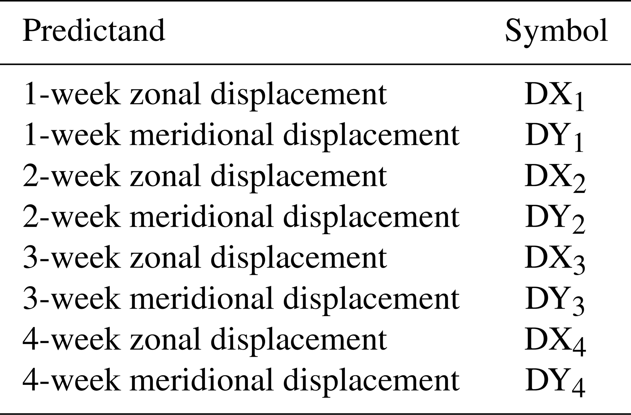
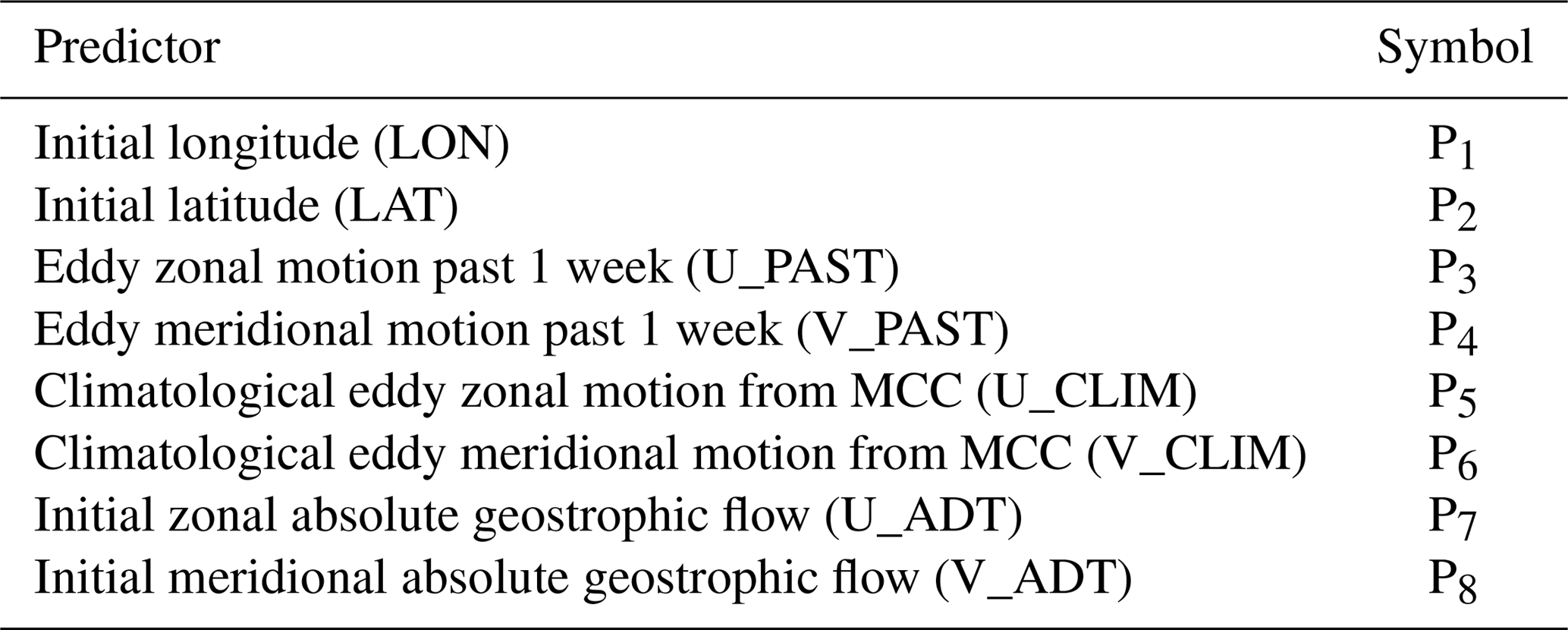
In this study, the predictands (dependent variables) are the zonal and meridional displacements from the initial positions at each forecast time (Table 1). The choice of the predictors based on physical analysis are shown in detail in Sect. 3. Since the variables used for the regression involve different scales and units, it is inappropriate to use them directly as it may cause the fitting to deviate from the physical constraints. Thus, all the variables are normalized with their anomalies divided by their corresponding standard deviations before the regressing. After that, the normalized predicted zonal (meridional) displacement DX (DY) can be estimated using a multiple linear regression method:
where the subscript j refers to the forecasting interval (1–4 weeks), the subscript i refers to the serial number of normalized predictors (P), n represents the number of selected predictors; a and b denote the regression coefficients of predictors onto DX and DY, respectively.
There are a total of eight regression equations, i.e., both the meridional and zonal directions for the weeks 1–4. We separate the whole eddy trajectories into two sets: one for regressing and the other for forecasting. For week 1, we used 1981 (76 %) eddy trajectory segments (a segment is the distance between two neighboring eddy center positions at 7-day intervals on a single eddy trajectory) of 283 eddy trajectories during 1992–2008 for regressing, and 623 (24 %) eddy trajectory segments of 81 eddy trajectories during 2009–2013 for forecasting. The other forecast experiments for 2, 3, and 4 weeks maintain the same periods for regressing and forecasting. To evaluate the overall forecasting ability of the model, the mean forecasting error is defined as the averaged distance (D) between the predicted eddy positions and the satellite observed eddy positions following the great circle distance (Ali et al., 2007):
where R is the earth radius, Xo (XF) and Yo(YF) represent the observed (predicted) longitude and latitude in degrees, respectively.
3.1 Pattern and dynamical analysis of eddy propagation in the NSCS
One of the most important steps in the development of a regression model is the choice of independent variables (predictors). In choosing the potential predictors, the candidates should have a physical link (direct or indirect) with the eddy propagation. To investigate the dynamical factors associated with eddy propagation in the NSCS, the pattern of eddy propagation speeds should be estimated first.
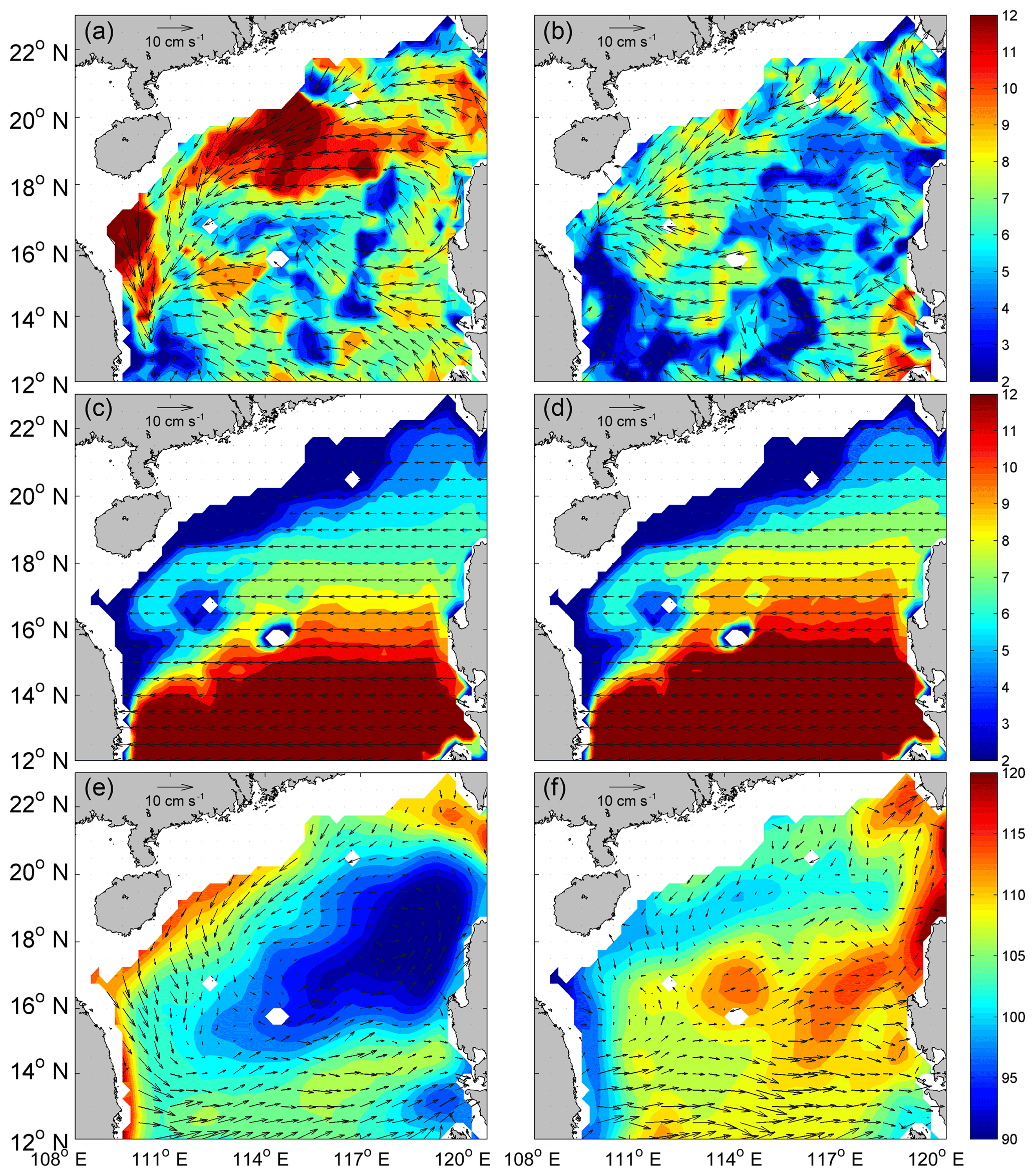
Figure 2Winter climatology of (a) eddy propagation speed directions (vectors) and magnitudes (color, cm s−1). (c) The phase speed directions (vectors) and magnitudes (color, cm s−1) of the first baroclinic Rossby wave. (e) The speed difference (vectors) between (a) and (c) superimposed on the winter mean absolute dynamic topography (color, cm). (b), (d) and (f) are the same as (a), (c) and (e), respectively, but represent the summer season.
Instead of a Lagrangian description of the movement of individual eddies as reported in the previous studies (e.g., Wang et al., 2003; Chen et al., 2011), the space–time-lagged MCC method provides an Eulerian description of the pattern of eddy propagation speeds (Fu, 2009). As shown in Fig. 2a and d, the MCC method has mapped the propagation speeds of eddies in the NSCS for the winter and summer seasons, respectively. The propagation of eddies is generally westward in the ocean interior and southward in the western boundary with a typical speed of 4–10 cm s−1. The propagation direction of eddies generated southwest of Taiwan is southwestward along the 200–2000 m isobaths, indicating the steering effects of the ocean's bathymetry. There are two distinct differences between the winter season and the summer season: one is that the eddy propagation speed in winter is relatively larger than that in summer; and the other is that the influence of the western boundary current can be clearly seen near 16–18∘ N along the Vietnam coast only in winter, creating an organized band of a southward eddy propagation pattern. The different patterns of the eddy propagation speed in winter and summer have revealed several details of the mean flow in the NSCS: the large-scale circulation under the influence of northeasterly winter monsoon is stronger than that in the southwesterly summer monsoon, and the robust western boundary current in winter becomes relatively weak and unorganized in summer.
Eddies also have their own westward drift under the planetary β effect in the absence of any mean flow (Nof, 1981; Cushiman-Roisin, 1994). Their propagation speed is approximately the phase speed of the first baroclinic Rossby waves with preferences for small poleward and equatorward deflection of cyclonic and anticyclonic eddies in the global ocean, respectively (Chelton et al., 2007). Theoretically, the phase speed of the first baroclinic Rossby wave is , where the first baroclinic Rossby radius of deformation R1 is estimated using the climatological GDEM temperature and salinity data. Figure 2c and d show the theoretical phase speed of nondispersive baroclinic Rossby waves calculated from GDEM winter (summer) climatological temperature and salinity data. The direction of the phase speed is due west and the magnitude increases from about 2 cm s−1 in the north latitude to 12 cm s−1 in the south latitude. It should be noted that the difference between the winter and summer distributions of the phase speed of the first baroclinic Rossby wave is relatively small. The underlying reason is that the variation of seasonal stratification in the upper layer has little effect on the seasonal distribution of the first baroclinic Rossby deformation radius (Chelton et al., 1998; Cai et al., 2008).
The differences between the satellite observed propagation speed (Fig. 2a and b) and the propagation speed induced by the β effect (Fig. 2c and d) in winter and summer are shown in Fig. 2e and f, respectively, which may represent the propagation speed caused by the advection of the mean flow. To further illustrate the advection effect of the mean flow, the winter (summer) mean dynamic topography is superimposed on the propagation speed caused by the mean flow. As can be seen, there is a good spatial correlation (0.61 in the zonal direction and 0.52 in the meridional direction, both of which are significant at the 95 % confidence level) between the cyclonic eddy propagation speed advected by the mean flow and the large-scale surface cyclonic circulation in winter, both of which are centered northwest of the Luzon Island (Fig. 2e). Due to the weak cyclonic gyre in the NSCS, the spatial correspondence in summer (Fig. 2f) is not as obvious as that in winter. Since the propagation speed induced by the β effect is westward, this tendency is reinforced by the mean flow in the north, but compensated by the mean flow in the south. Because the mean flow in the south is not so strong, it is not able to reverse eddy propagation from its westward motion induced by the β effect, as in the Antarctic Circumpolar Current region (Klocker and Marshall, 2014), no matter if it is winter or summer.
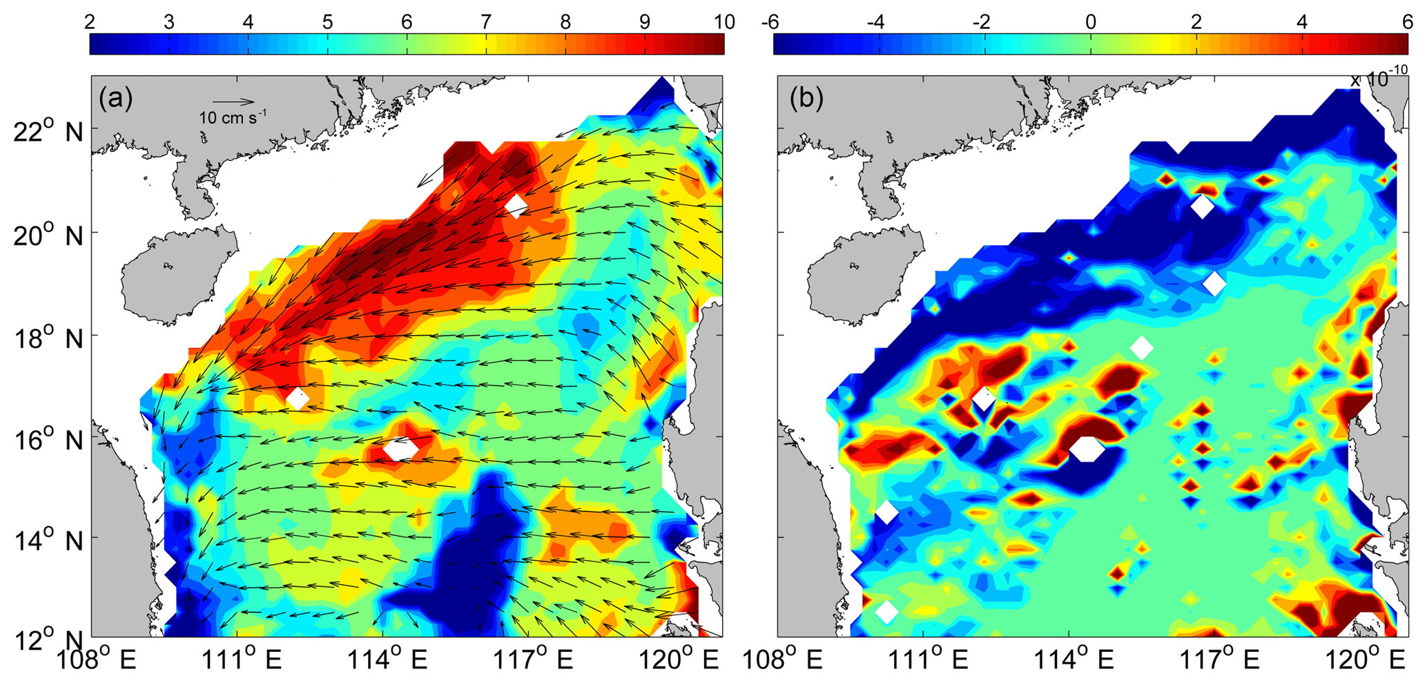
Figure 3(a) Annual mean of eddy propagation speed directions (vectors) and magnitudes (color, cm s−1). (b) Meridional distribution of the topographic β effect (color shading).
To explore other possible causes of eddy propagation, Fig. 3a shows the annual mean eddy propagation speed. The most striking pattern is that the eddy propagation speed is markedly accelerated on the northern continental shelf of the NSCS (also can be seen in Fig. 2a and b), which corresponds well to the region of negative maximum meridional topographic , where H is the water depth. Their correlation is −0.40, which is significant at the 95 % confidence level. This relatively good correspondence suggests that besides the planetary β effect and advection of mean flow, the topographic β effect also contributes to the eddy propagation in some regions where the bathymetry gradient cannot be neglected.
3.2 Choice of predictors
As mentioned above, the mean flow advection and the effects of β (both planetary and topographic) are closely related with the eddy propagation. These factors should be considered as the potential predictors, and the seasonal climatological eddy zonal and meridional motions (U_CLIM, V_CLIM) derived from the MCC are calculated to represent the effects of β and the mean flow advection. Note that we have tried to decompose U_CLIM and V_CLIM into the effects of β and the mean flow advection, and to incorporate them into the regression model, but found no improvement in the forecasting skill.
In reality, the large-scale circulation evolves during the forecast period; this synoptic effect of mean flow advection should also be taken into account. To help account for the time variation of the mean flow advection, the current zonal and meridional absolute geostrophic flows (U_ADT, V_ADT) derived from the satellite data are evaluated at the beginning of the forecast time along the eddy trajectory. Besides, the persistence factors should also be considered in the regression model, since they contain the “latest” pattern of eddy propagation under the effects of β and the mean flow advection. The chosen persistence factors are the initial eddy position (LON, LAT) and the eddy motion past 1 week (U_PAST, V_PAST). All the chosen eight predictors are listed in Table 2 and can be derived along the eddy trajectories. They can be divided into two categories: (1) P1–P6 related to climatology and persistence, i.e., “static predictors”, and (2) P7–P8 related to the changing environmental conditions, i.e., “synoptic predictors”.
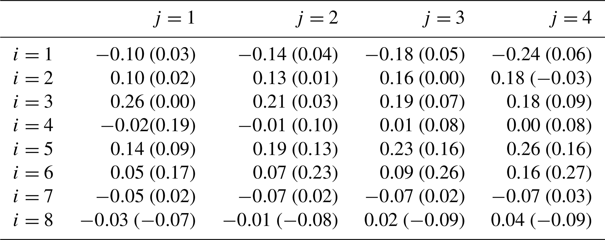
The relative contribution of each predictor on each forecasting period is illustrated by the normalized regression coefficient (Table 3). The larger the normalized regression coefficient, the greater its contribution to the individual forecast equation. Persistence factors (U_PAST, V_PAST) are initially the most important predictors, while after 2 weeks the most important predictors are the climatology factors (U_CLIM, V_CLIM). The synoptic predictors (U_ADT, V_ADT) contribute less to the forecast equations compared to persistence and climatology. The underlying reason may be that the week to week variations are too large, so the representation of the initial U_ADT and V_ADT to the actual velocities in the 4-week window is not as good as the U_CLIM and V_CLIM representation.
Table 3Normalized regression coefficients ai,j (bi,j) for use with the eddy zonal (meridional) motion prediction equation.
4.1 Comparison to the persistence method
To evaluate the performance of our prediction model, the persistence method and our model are used to predict the eddy trajectories during 2009–2013. The persistence method is a benchmark comparison and forecast reference widely accepted in the atmospheric and oceanic sciences (Mittermaier, 2008; Müller et al., 2012), which is defined as , where χ is any parameter, and t is a distance time step. In this study, χ refers to the eddy propagation speed and the persistence means no change of propagation speed from the initial state (Fig. 4a). The root mean square error (RMSE) and correlation coefficient between the predicted and actual longitudes (latitudes), and the mean distance errors of our model and the persistence method over a 4-week horizon are computed.
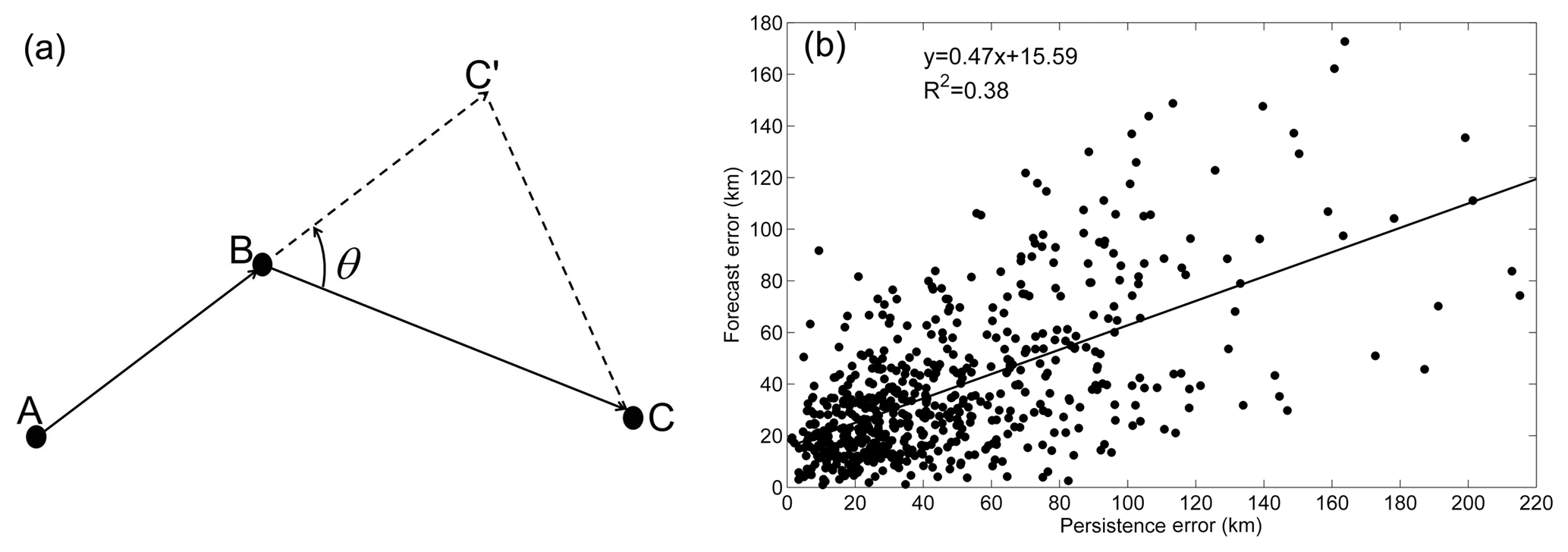
Figure 4(a) Schematic of the persistence method. A, B, and C are three observed eddy positions on the trajectory at each 1-week interval. C' is the predictive eddy position 1 week in advance by the persistence method; BC' = AB. Thus CC' is the persistence error at week 1. (b) Scatterplot of persistence error versus forecast error of our model at week 1 with a best fit linear regression.
Table 4 lists the comparison of prediction results. It shows that our multiple linear regression model beats the persistence method and indicates our model has some forecasting skill (Table 5): the RMSE between the predicted and the actual longitudes (latitudes) throughout the 4-week horizon is 32.7–89.2 km (29.5–73.5 km) with the correlation coefficients > 0.93 (> 0.95).
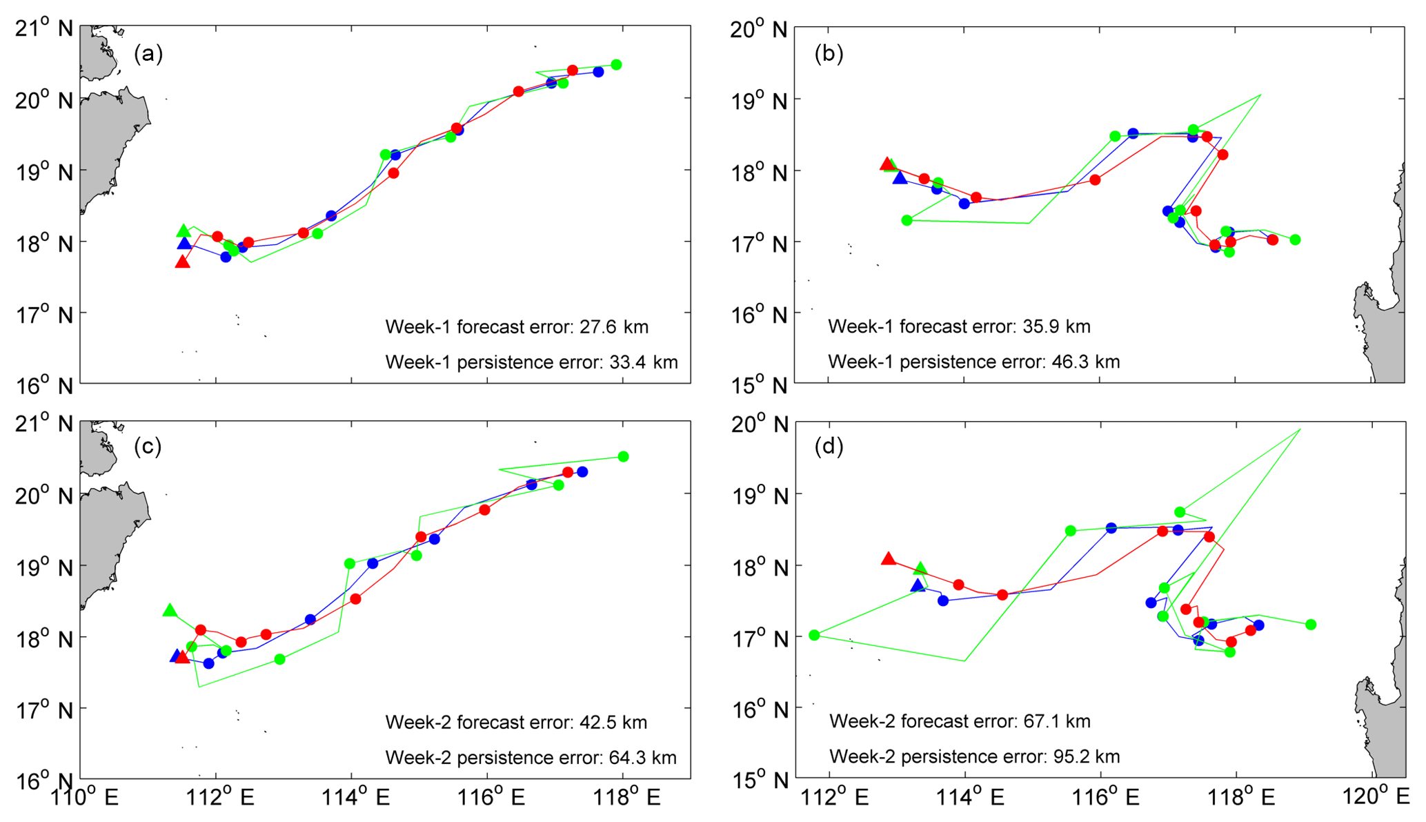
Figure 5A comparison of the satellite observed trajectory (red), the trajectory predicted by our model (blue) and persistence trajectory (green) at (a) week 1 and (c) week 2. (b) and (d) are the same as (a) and (c), respectively, but for a recurved trajectory. The biweekly eddy positions of each trajectory are shown by the solid circles. The ending position of each trajectory is represented by the solid triangle.
Table 4Comparison of the mean forecast distance errors (km) of the persistence, multiple linear regression (MLR), and artificial neural network (ANN) methods.

As an example, Fig. 5 compares the 1–2 weeks forecasting performances of our model (blue) and the persistence method (green) with the observation (red). Generally, the eddy trajectory predicted 1–2 weeks in advance by our model coincides well with the observed trajectory with an overall average error of 27.6 km (week 1) and 42.5 km (week 2). Even the convoluted pattern can be reproduced properly (Fig. 5b, and d) though the mean error is slightly larger than in the smooth case. In contrast, although the persistence forecast trajectory at week 1 is relatively consistent with the observed trajectory (Fig. 5a and b), the persistence method cannot forecast the eddy trajectories properly when the forecast horizon increases (Fig. 5c and d). To further compare their differences, their forecast distance errors are normalized with the Rossby radius on each forecast grid over a 4-week forecast window, respectively. The correlation between the normalized forecast distance errors of the persistence method and our model decreases from 0.67 at week 1 to 0.38 at week 4. This is consistent with the above judgement and confirms the superiority of our multiple linear regression model over the persistence method.
Table 5Statistics of our multiple linear regression model for different forecast times of eddy propagation positions in terms of longitude (latitude).
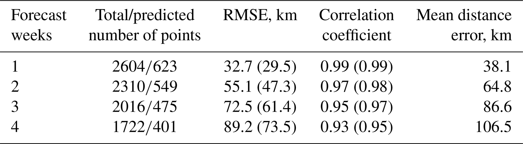
Note: the total/predicted number of points refers to the eddy positions at 7-day time intervals in the total/predicted eddy trajectories during 1992–2013/2009–2013; the RMSE is the root mean square error between the predicted and the observed longitude (latitude).
4.2 Sensitive performance of different eddy polarities and the season
Previous studies have shown that anticyclonic eddies and cyclonic eddies in the NSCS have different dynamic characteristics, such as generation sites, rotation speeds, and propagation trajectories; and the seasonal variability of these eddies is robust (Wang et al., 2006, 2008; Li et al., 2011). Two natural questions arise: (1) is there any difference on the model forecast ability between anticyclonic eddies (Fig. 1a) and cyclonic eddies (Fig. 1b)? (2) If so, is there any difference on the forecasting ability for one type of eddy in winter (Figs. 7a and 8a) and summer (Figs. 7b and 8b)? This section will explore the different model performances for two types of eddies during different seasons in the NSCS.

Figure 6Comparison of the mean forecast errors between anticyclonic eddies (red) and cyclonic eddies (blue) over a 4-week window.
The period considered for regressing and predicting the anticyclonic eddy and cyclonic eddy positions is the same as that used in developing the predictive model (see Sect. 2.3). The mean forecast errors of anticyclonic (cyclonic) eddies from week 1 to week 4 are 36.9 km (41.1 km), 62.6 km (68.1 km), 81.0 km (88.5 km), and 102.0 km (108.2 km), respectively (Fig. 6). These results show that the forecast errors of anticyclonic eddies are smaller than those of cyclonic eddies in all forecast horizons, and the maximum error difference can reach 7.5 km at week 3. To investigate the underlying reasons of different model performances for anticyclonic eddies and cyclonic eddies, we use the persistence error ( in Fig. 4a) at week 1 as an index to measure the difficulty of trajectory forecast. The underlying reason in physics is that CC', which includes the effects of the winding angle (θ, measuring the trajectory curvature) and the eddy propagation distances in the last week and the next week (AB and BC, measuring the eddy propagation speed), is an integral characteristic of the eddy trajectory. The correlation between this integrated index and the eddy trajectory forecast error is relatively high with R=0.62 (Fig. 4b), which is significant at the 95 % confidence level and shows its ability in measuring the inherent difficulty of a trajectory forecast: the larger the index, the more difficult the trajectory forecast, thus the larger the forecast error. Because the indices (mean persistence errors) of all the anticyclonic and cyclonic eddy trajectories in the NSCS are 46.6 and 53.0 km, respectively, it is not difficult to understand why the mean forecast error of anticyclonic eddy trajectories is smaller than that of cyclonic eddy trajectories in the NSCS. The index difference between anticyclonic and cyclonic eddy trajectories is caused by these different trajectory patterns (Fig. 1a and b), which could be due to the opposing meridional drifts of anticyclonic and cyclonic eddies expected from the combination of the β effect and self-advection (Morrow et al., 2004).
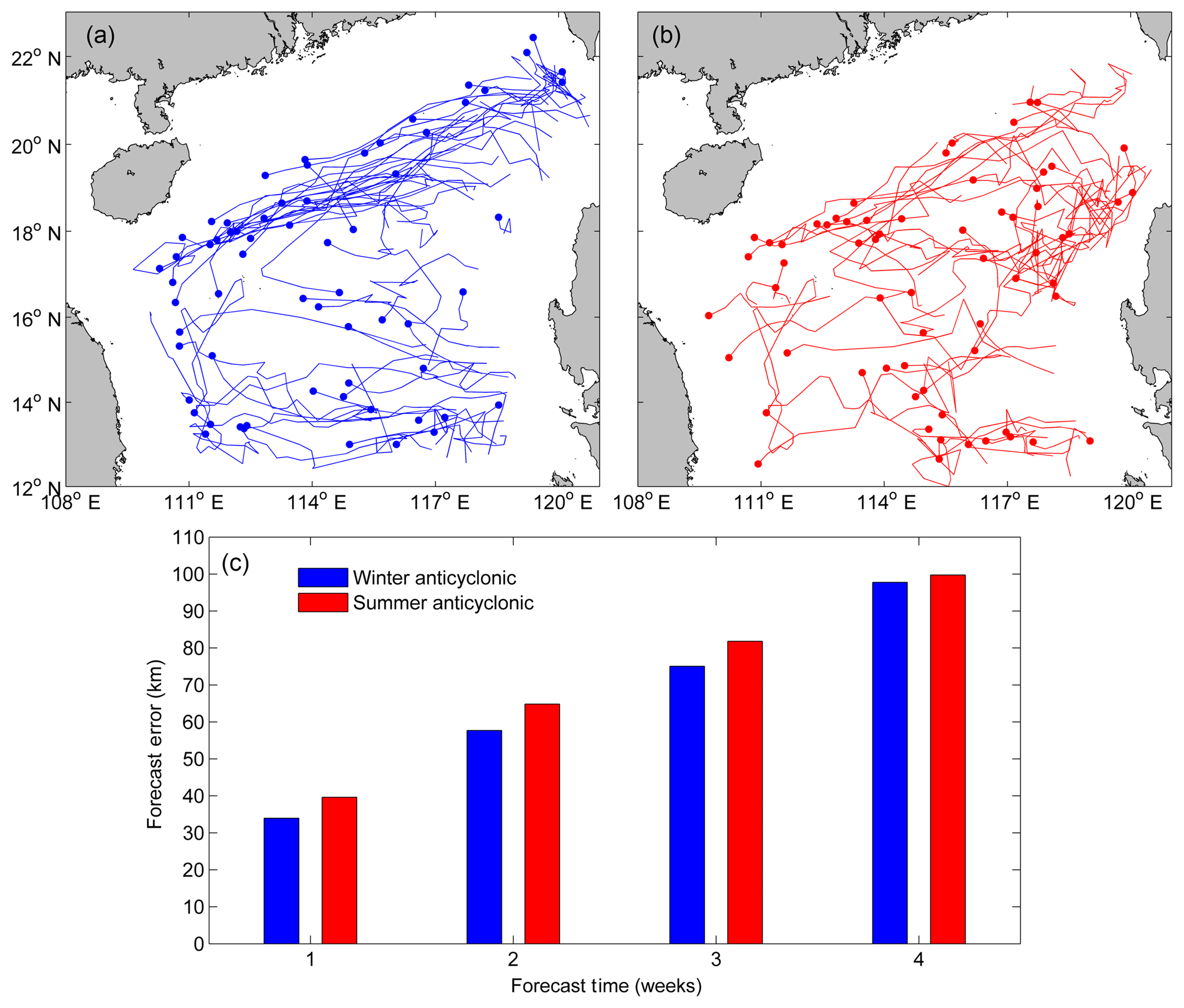
Figure 7The trajectories of anticyclonic eddies in (a) winter and (b) summer with lifetime ≥ 5 weeks in the northern South China Sea. The solid circle represents the ending position of each trajectory. (c) Comparison of their mean forecast errors over a 4-week window.

Figure 7c (Fig. 8c) shows the mean forecast errors of anticyclonic (cyclonic) eddy trajectories in winter and summer over a 4-week horizon. Because the mean persistence error (42.0 km) of anticyclonic eddy trajectories in winter is smaller than that (51.9 km) in summer, as expected, the mean forecast error of anticyclonic eddy trajectories in winter is smaller than that in summer for all cases. This is also the case for the cyclonic eddy: since the mean persistence error (54.6 km) of cyclonic eddy trajectories in winter is relatively larger than that (52.8 km) in summer, the mean forecast error of the cyclonic eddy trajectories in winter is larger than that in summer. The index difference of one type of eddy trajectory between winter and summer is also caused by the different trajectory patterns. Why do the anticyclonic and cyclonic eddies follow different trajectories in winter (Figs. 7a and 8a) and summer (Fig. 7b and b)? One possible dynamical reason is the different interactions between the eddies and seasonal mean flows. Other underlying factors such as eddy generation mechanisms and eddy-topography interactions in different seasons may also contribute. This is beyond the scope of this study and needs further investigation using numerical models.
In this study, we have investigated the underlying dynamics of the eddy propagation in the NSCS and found their propagation is mainly driven by the combination of the planetary β effect and mean flow advection. In addition, the topographic β effect also has some contribution to the eddy propagation where the bathymetry gradient cannot be neglected, like the steep continental shelf in the NSCS (Fig. 1a).
Based on dynamical analysis, predictors were chosen and a simple statistical predictive model for relating various oceanic parameters to eddy propagation position changes was developed using the multiple linear regression method. This predictive model is made up of eight predictands (zonal and meridional displacements over 1–4 weeks) and eight predictors (six static predictors, two synoptic predictors). The six static predictors are associated with the initial position, the zonal and meridional motions past 1 week, and the climatological eddy zonal and meridional motions. The other two synoptic predictors account for the time variation of the mean flow advection. Results showed that this simple model has significant forecasting skills over a 4-week forecast horizon compared to the traditional persistence method. Moreover, the model performance is sensitive to the eddy type and the forecast season: (1) the predicted trajectory errors of anticyclonic eddies are smaller than those of cyclonic eddies, and (2) the predicted trajectory errors of anticyclonic eddies in winter are smaller than those in summer; while the contrary is the case for the cyclonic eddy. The predictive model performance strongly depends on the inherent difficulty of the trajectory forecast.
Although the performance of the proposed predictive model is encouraging, it could be refined further. Further improvement may be possible by including the effect of eddy–eddy interactions on the eddy propagation, which is supposed to help induce the eddy trajectory curve or loop (Early et al., 2011). Another possible improvement is to use artificial neural network (ANN) in developing the forecast model. ANN has been successfully used in predicting cyclone tracks (Ali et al., 2007) and loop current variation (Zeng et al., 2015). ANN can represent both linear and non-linear relationships learned directly from the data being modeled. It mainly contains three layers: the input layer, the hidden layer, and the output layer. To be consistent with the multiple linear regression model, both the input layer and the output layer include the same predictors and predictands as the regression model, respectively. The hidden layer consists of two layers of neural variables. Through iterations on backward propagation of the error, the neural network learns by itself to achieve an optimum weighting function and a minimum error. The forecast errors of ANN for 1–4 weeks are listed in Table 4. We can see that some improvements (0.3–4.2 km during 1–4 weeks forecast horizon) have been shown compared to the linear regression method. Recently, Jiang et al. (2018) have found that the deep-learning algorithm of neural networks performs better than the simple ANN for the parameterization of typhoon–ocean feedback in typhoon forecast models. These enhancements (both physics and algorithms) are topics warranting future research and development.
The SLA and MDT data can be downloaded from AVISO (ftp://ftp.aviso.oceanobs.com/, Ducet et al., 2000), and the NSCS eddy trajectory data can be derived from the third release global eddy dataset (http://cioss.coas.oregonstate.edu/eddies/, Chelton et al., 2011).
JL performed the data analyses and wrote the manuscript. GW planned the research and co-wrote the manuscript. HX and HW contributed to interpretation of the results and improving the manuscript.
The authors declare that they have no conflict of interest.
This work is supported by the National Key Research and Development Program of China (2017YFC1404103), the National Natural Science Foundation of China (41811530301 and 41621064), the National Programme on Global Change and Air-Sea Interaction (GASI-IPOVAI-04), the Program of Shanghai Academic/Technology Research Leader (17XD1400600), and the China Postdoctoral Science Foundation (2016M601493). We wish to thank the editor and the two anonymous reviewers for their valuable suggestions and comments.
This paper was edited by Matthew Hecht and reviewed by two anonymous referees.
Aberson, S. D. and Sampson, C. R.: On the predictability of tropical cyclone tracks in the northwest pacific basin, Mon. Wea. Rev., 131, 1491–1497, 2003.
Ali, M. M., Kishtawal, C. M., and Jain, S.: Predicting cyclone tracks in the north Indian Ocean: An artificial neural network approach, Geophys. Res. Lett., 34, L04603, https://doi.org/10.1029/2006GL028353, 2007.
Bao, S., Zhang, R. Wang, H., Yan, H., and Yu, Y.: Salinity profile estimation in the Pacific Ocean from satellite Surface salinity observations, J. Atmos. Oceanic. Technol., 36, 53–68, 2019.
Cai, S., Long, X., Wu, R., and Wang, S.: Geographical and monthly variability of the first baroclinic rossby radius of deformation in the south china sea, J. Mar. Syst., 74, 711–720, 2008.
Canes, M. R.: Description and evaluation of GDEM-V3.0, Rep. NRL/MR/7330-09-9165, Nav. Res. Lab, Washington, DC, 2009.
Chelton, D., DeSzoeke, R., and Schlax, M.: Geographical variability of the first baroclinic rossby radius of deformation, J. Phys. Oceanogr., 28, 433–460, 1998.
Chelton, D. B., Schlax, M. G., Samelson, R. M., and de Szoeke, R. A.: Global observations of large oceanic eddies, Geophys. Res. Lett., 34, L15606, https://doi.org/10.1029/2007GL030812, 2007.
Chelton, D. B., Schlax, M. G., and Samelson, R. M.: Global observations of nonlinear mesoscale eddies, Prog. Oceanogr., 91, 167–216, https://doi.org/10.1016/j.pocean.2011.01.002, 2011 (data available at: http://cioss.coas.oregonstate.edu/eddies/, last access: 30 March 2017).
Chen, G., Hou, Y., and Chu, X.: Mesoscale eddies in the South China Sea: Mean properties, spatiotemporal variability, and impact on thermohaline structure, J. Geophys. Res., 116, C06018, https://doi.org/10.1029/2010JC006716, 2011.
Cushiman-Roisin, B.: Introduction to Geophysical Fluid Dynamics, Prentice Hall, 320 pp., 1994.
Demaria, M. and Kaplan, J.: A statistical hurricane intensity prediction scheme (SHIPS) for the Atlantic basin, Weather Forecast., 9, 209–220, 1994.
Dominiak, S. and Terray, P.: Improvement of ENSO prediction using a linear regression model with a southern Indian Ocean sea surface temperature predictor, Geophys. Res. Lett., 32, L18702, https://doi.org/10.1029/2005GL023153, 2005.
Dong, C., Mcwilliams, J. C., Liu, Y., and Chen, D.: Global heat and salt transports by eddy movement, Nat. Commun., 5, 3294, https://doi.org/10.1038/ncomms4294, 2014.
Ducet, N., Le Traon, P. Y., and Reverdin, G.: Global high-resolution mapping of ocean circulation from TOPEX/Poseidon and ERS-1 and -2, J. Geophys. Res., 105, 19477–19498, https://doi.org/10.1029/2000JC900063, 2000 (data available at: ftp://ftp.aviso.oceanobs.com/, last access: 20 November 2018).
Early, J. J., Samelson, R. M., and Chelton, D. B.: The evolution and propagation of quasigeostrophic ocean eddies, J. Phys. Oceanogr., 41, 1535–1555, 2011.
Emery, W. J., Thomas, A. C., Collins, M. J., Crawford, W. R., and Mackas, D. L.: An objective method for computing advective surface velocities from sequential infrared satellite images, J. Geophys. Res., 91, 12865–12878, https://doi.org/10.1029/JC091iC11p12865, 1986.
Fu, L.-L.: Pathways of eddies in the South Atlantic Ocean revealed from satellite altimeter observations, Geophys. Res. Lett., 33, L14610, https://doi.org/10.1029/2006GL026245, 2006.
Fu, L.-L.: Pattern and speed of propagation of the global ocean eddy variability, J. Geophys. Res., 114, C11017, https://doi.org/10.1029/2009JC005349, 2009.
Hurlburt, H., Chassignet, E., Cummings, J., Kara, A., Metzger, E., Shriver, J., Smedstad, O., Wallcraft, A., and Barron., C.: Eddy Resolving Global Ocean Prediction, Washington DC, American Geophysical Union Geophysical Monograph Series, 353–381, https://doi.org/10.1029/177GM21, 2008.
Jiang, G.-Q., Xu, J., and Wei, J.: A deep learning algorithm of neural network for the parameterization of typhoon-ocean feedback in typhoon forecast models, Geophys. Res. Lett., 45, 3706–3716, https://doi.org/10.1002/2018GL077004, 2018.
Klocker, A. and Marshall, D. P.: Advection of baroclinic eddies by depth mean flow, Geophys. Res. Lett., 41, 3517–3521, https://doi.org/10.1002/2014GL060001, 2014.
Leese, J. A., Novak, C. S., and Clark, B. B.: An automated technique for obtaining cloud motion from geosynchronous satellite data using cross correlation, J. Appl. Meteor., 10, 118–132, 1971.
Li, J., Zhang, R., and Jin, B.: Eddy characteristics in the northern South China Sea as inferred from Lagrangian drifter data, Ocean Sci., 7, 661–669, https://doi.org/10.5194/os-7-661-2011, 2011.
Li, J., Wang, G., and Zhai, X.: Observed cold filaments associated with mesoscale eddies in the South China Sea, J. Geophys. Res.-Oceans, 122, 762–770, https://doi.org/10.1002/2016JC012353, 2017.
Liu, W. T. and Xie, X.: Space-based observations of the seasonal changes of South Asian monsoons and oceanic response, Geophys. Res. Lett., 26, 1473–1476, 1999.
Ma, X., Jing, Z., Chang, P., Liu, X., Montuoro, R., Small, R. J., Bryan, F. O., Greatbatch, R. J., Brandt, P., Wu, D. X., Lin, X. P., and Wu, L. X.: Western boundary currents regulated by interaction between ocean eddies and the atmosphere, Nature, 535, 533–537, 2016.
Matear, R. J. and McNeil, B. I.: Decadal accumulation of anthropogenic CO2 in the Southern Ocean: A comparison of CFC-age derived estimates to multiple-linear regression estimates, Global Biogeochem. Cy., 17, 1113, https://doi.org/10.1029/2003GB002089, 2003.
Morrow, R., Birol, F., Griffin, D., and Sudre, J.: Divergent pathways of cyclonic and anti-cyclonic ocean eddies, Geophys. Res. Lett., 31, L24311, https://doi.org/10.1029/2004GL020974, 2004.
Mittermaier, M.: The potential impact of using persistence as a reference forecast on perceived forecast skill, Weather Forecast., 23, 1022–1031, 2008.
Müller, W. A., Baehr, J., Haak, H., Jungclaus, J. H., Kröger, J., Matei, D., Notz, D., Pohlmann, H., von Storch, J. S., and Marotzke, J.: Forecast skill of multi-year seasonal means in the decadal prediction system of the Max Planck Institute for Meteorology, Geophys. Res. Lett., 39, L22707, https://doi.org/10.1029/2012GL053326, 2012.
Ninnis, R. M., Emery, W. J., and Collins, M. J.: Automated extraction of pack ice motion from advanced very high resolution radiometer imagery, J. Geophys. Res., 91, 10725–10734, https://doi.org/10.1029/JC091iC09p10725, 1986.
Nof, D.: On the β-induced movement of isolated baroclinic eddies, J. Phys. Oceanogr., 11, 1662–1672, 1981.
Oey, L.-Y., Ezer, T., Forristall, G., Cooper, C., DiMarco, S., and Fan, S.: An exercise in forecasting loop current and eddy frontal positions in the Gulf of Mexico, Geophys. Res. Lett., 32, L12611, https://doi.org/10.1029/2005GL023253, 2005.
Rienecker, M. M., Mooers, C. N. K., and Robinson, A. R.: Dynamical interpolation and forecast of the evolution of mesoscale features off northern California, J. Phys. Oceanogr., 17, 1189–1213, 1987.
Rio, M.-H. and Hernandez, F.: A mean dynamic topography computed over the world ocean from altimetry, in situ measurements, and a geoid model, J. Geophys. Res., 109, C12032, https://doi.org/10.1029/2003JC002226, 2004.
Robinson, A. R., Carton, J. A., Mooers, C. N. K., Walstad, L. J., Carter, E. F., Rienecker, M. M., Smith, J. A., and Leslie, W. G.: A real-time dynamical forecast of ocean synoptic/mesoscale eddies, Nature, 309, 781–783, 1984.
Seo, K. H., Wang, W., Gottschalck, J., Zhang, Q., Schemm, J.-K., Higgins, W., and Kumar, A.: Evaluation of MJO Forecast Skill from Several Statistical and Dynamical Forecast Models, J. Climate, 22, 2372–2388, 2009.
Shaw, P. T.: Seasonal variation of the intrusion of the Philippine Sea water into the South China Sea, J. Geophys. Res., 96, 821–827, 1991.
Wang, G., Su, J., and Chu, P. C.: Mesoscale eddies in the South China Sea observed with altimeter data, Geophys. Res. Lett., 30, 2121, https://doi.org/10.1029/2003GL018532, 2003.
Wang, G., Chen, D., and Su, J.: Generation and life cycle of the dipole in the South China Sea summer circulation, J. Geophys. Res., 111, C06002, https://doi.org/10.1029/2005JC003314, 2006.
Wang, G., Chen, D., and Su, J.: Winter eddy genesis in the eastern South China Sea due to orographic wind-jets, J. Phys. Oceanogr., 38, 726–732, https://doi.org/10.1175/2007JPO3868.1, 2008.
Wang, G., Li, J., Wang, C., and Yan, Y.: Interactions among the winter monsoon, ocean eddy and ocean thermal front in the South China Sea, J. Geophys. Res., 117, C08002, https://doi.org/10.1029/2012JC008007, 2012.
Xiu, P., Chai F., Shi, L., Xue, H., and Chao, Y.: A census of eddy activities in the South China Sea during 1993–2007, J. Geophys. Res., 115, C03012, https://doi.org/10.1029/2009JC005657, 2010.
Zhang, R.: Meachanims for the low frequency of summer Arctic sea ice extent, P. Natl. Acad. Sci. USA, 112, 4570–4575, 2015.
Zhang, Z., Wang, W., and Qiu, B.: Oceanic mass transport by mesoscale eddies, Science, 345, 322–324, 2014.
Zeng, X., Li, Y., and He, R.: Predictability of the loop current variation and eddy shedding process in the Gulf of Mexico using an artificial neural network approach, J. Atmos. Oceanic. Technol., 32, 1098–1111, 2015.
Zhuang W., Du, Y., Wang, D., Xie, Q., and Xie, S.-P.: Pathways of mesoscale variability in the South China Sea, Chin. J. Oceanol. Limn., 28, 1055–1067, 2010.