the Creative Commons Attribution 4.0 License.
the Creative Commons Attribution 4.0 License.
 | 13 Aug 2019
High-resolution underwater laser spectrometer sensing provides new insights into methane distribution at an Arctic seepage site
Jack Triest
Bénédicte Ferré
Anna Silyakova
Jürgen Mienert
Jérôme Chappellaz
Methane (CH4) in marine sediments has the potential to contribute to changes in the ocean and climate system. Physical and biochemical processes that are difficult to quantify with current standard methods such as acoustic surveys and discrete sampling govern the distribution of dissolved CH4 in oceans and lakes. Detailed observations of aquatic CH4 concentrations are required for a better understanding of CH4 dynamics in the water column, how it can affect lake and ocean acidification, the chemosynthetic ecosystem, and mixing ratios of atmospheric climate gases. Here we present pioneering high-resolution in situ measurements of dissolved CH4 throughout the water column over a 400 m deep CH4 seepage area at the continental slope west of Svalbard. A new fast-response underwater membrane-inlet laser spectrometer sensor demonstrates technological advances and breakthroughs for ocean measurements. We reveal decametre-scale variations in dissolved CH4 concentrations over the CH4 seepage zone. Previous studies could not resolve such heterogeneity in the area, assumed a smoother distribution, and therefore lacked both details on and insights into ongoing processes. We show good repeatability of the instrument measurements, which are also in agreement with discrete sampling. New numerical models, based on acoustically evidenced free gas emissions from the seafloor, support the observed heterogeneity and CH4 inventory. We identified sources of CH4, undetectable with echo sounder, and rapid diffusion of dissolved CH4 away from the sources. Results from the continuous ocean laser-spectrometer measurements, supported by modelling, improve our understanding of CH4 fluxes and related physical processes over Arctic CH4 degassing regions.
- Article
(5214 KB) - Full-text XML
-
Supplement
(428 KB) - BibTeX
- EndNote


Methane (CH4) release from gas-bearing ocean sediments has been of high interest for many years (e.g. Westbrook et al., 2009; Ferré et al., 2012; Ruppel and Kessler, 2016; Jørgensen et al., 1990; Boetius and Wenzhöfer, 2013; Myhre et al., 2016; Platt et al., 2018). Once released and dissolved in the water column, the CH4 gas diffuses and is partly oxidized in the water column (Reeburgh, 2007), contributing to minimum oxygen zones (Boetius and Wenzhöfer, 2013) and possibly to ocean acidification (Biastoch et al., 2011). Chemosynthetic life on the seabed depends on the supply of methane as an energy resource (e.g. Boetius and Wenzhöfer, 2013). Supply of nutrient-rich bottom water, by means of local upwelling, may enhance biological productivity and induce drawdown of CO2 from the atmosphere, potentially making shallow CH4 seepage sites sinks for this critical greenhouse gas (Pohlman et al., 2017). Warming of ocean bottom waters, active tectonics, and ice sheet build up and retreat could, at different timescales, lead to CH4 gas release from the seabed (e.g. Portnov et al., 2016). The magnitude and trend of such a phenomenon are still under debate (e.g. Hong et al., 2018; Ruppel and Kessler, 2016; Andreassen et al., 2017) and accurate methods to measure methane concentrations from its source are needed. At shallow seepage sites, such as the East Siberian Arctic Shelf, CH4 can potentially reach the atmosphere and amplify global warming (Shakhova et al., 2010, 2014). However, most studies of shallow CH4 seepage sites have found no or little CH4 flux to the atmosphere (e.g. Miller et al., 2017; Platt et al., 2018; Myhre et al., 2016; Gentz et al., 2014).
In the past, most CH4 measurements relied on indirect or discrete sample measurements (e.g. Damm et al., 2005; Westbrook et al., 2009; Gentz et al., 2014). Bubble catcher measurements as well as mapping with multibeam echo sounder (Sahling et al., 2014) and hydro-acoustic imaging together with bubble size and bubble rising speed measurements (Sahling et al., 2014; Weber et al., 2014; Veloso et al., 2015; Greinert et al., 2006; Ostrovsky, 2003) have been used to derive CH4 flow rates. The acoustic method effectively maps CH4 seepage from acoustically detectable sources and camera-equipped remotely operated vehicles (ROVs) can investigate their properties. However, these methods cannot detect CH4 from sources other than free gas seepage and do not provide information about the distribution of dissolved CH4. Discrete sampling with Niskin bottles allows 3-D mapping of dissolved CH4, but is limited by its labour intense nature, with resulting low resolution, which in turn may lead to smoothing and inaccurate estimates of CH4 inventories. The combination of bubble catcher and multibeam echo sounder measurements is very efficient once the bubble seepage has been properly categorized but uncertainties arise while extrapolating bubble catcher flow rates to acoustically evidenced bubble streams (flares). Present commercial underwater CH4 sensors do not have the required response time for accurate high-resolution mapping. For this reason, Gentz et al. (2014) deployed an underwater membrane-inlet mass spectrometer (UWMS) with a fast response time for mapping of CH4 at shallow (10 m) depths. Boulart et al. (2013) used an in situ real-time sensor in the Baltic Sea. The instrument response time of 1–2 min and detection limit of 3 nmol L−1 represent limitations for fast profiling and near-surface concentration studies linked to atmospheric exchange. Sommer et al. (2015) used a pump-fed membrane-inlet mass spectrometry installation at a blowout location in the North Sea. They achieved a response time of 30 min and a detection limit of 20 nmol L−1. Wankel et al. (2010) deployed a deep-sea graded in situ mass spectrometer over a brine pool in the Gulf of Mexico, where they measured high (up to 33 mM) concentrations of CH4. They do not specify their detection limit or the response time of the instrument but state an uncertainty of 11 %. Boulart et al. (2017) mapped hydrothermal activity while deploying an in situ mass spectrometer (ISMS) over the Southeast Indian Ridge. The ISMS has the advantage of measuring several dissolved gases simultaneously but only CH4 was reported because of the high detection limit of H2. The ISMS response time and detection limits were not specified.
Here we present the first in situ high-resolution ocean laser spectroscopy mapping of dissolved CH4 in seawater over active CH4 seepage in the Arctic. The data were collected by deploying a patented (patent France no. 17 50063) membrane-inlet laser spectrometer (MILS) (Grilli et al., 2018). The high-resolution measurements, together with echo-sounder data, discrete water sampling, and newly developed control volume and 2-dimensional (2-D) models, improve our understanding of CH4 fluxes from the seabed into oceans and lakes, and potentially to the atmosphere.
2.1 Study area
The survey was performed on board R/V Helmer Hanssen, UiT, The Arctic University of Norway, in October 2015 (CAGE 15-6 cruise) west of Prins Karls Forland located offshore western Svalbard. Over a period of 3 d (21–23 October), we surveyed an area of ∼18 km2 at water depths between 350 and 420 m using continuous underwater laser spectroscopy as well as traditional discrete sampling for dissolved CH4 and echo-sounding for bubble detection and gas seepage quantification. The study area is located at 78∘33′ N, 9∘30′ E over an active CH4 venting area (Fig. 1a). Here, more than 250 flares (acoustic signature of bubble streams in echograms) exist along the shelf break (e.g. Sahling et al., 2014; Westbrook et al., 2009; Damm et al., 2005; Graves et al., 2015; Berndt et al., 2014). The northward flowing West Spitsbergen Current (WSC), which transports Atlantic Water (AW, S>34.9, T>3 ∘C) (Schauer et al., 2004), controls the hydrography of the study area. The East Spitsbergen Current (ESC) flows southwestward along the eastern Spitsbergen coast and northward along the western Svalbard margin, carrying Arctic Surface Water (ASW, 34.4⩽S⩽34.9) and Polar Water (PW, S<34.4) (Skogseth et al., 2005). The Coastal Current (CC), extension of the ESC (Loeng, 1991; Skogseth et al., 2005), contributes a transient addition of ASW and PW on the shelf and the continental slope as the WSC meanders on- and offshore (Steinle et al., 2015). The Lower Arctic Intermediate Water (LAIW, S>34.9, T⩽3 ∘C) flows below the Atlantic Water (Ślubowska-Woldengen et al., 2007).
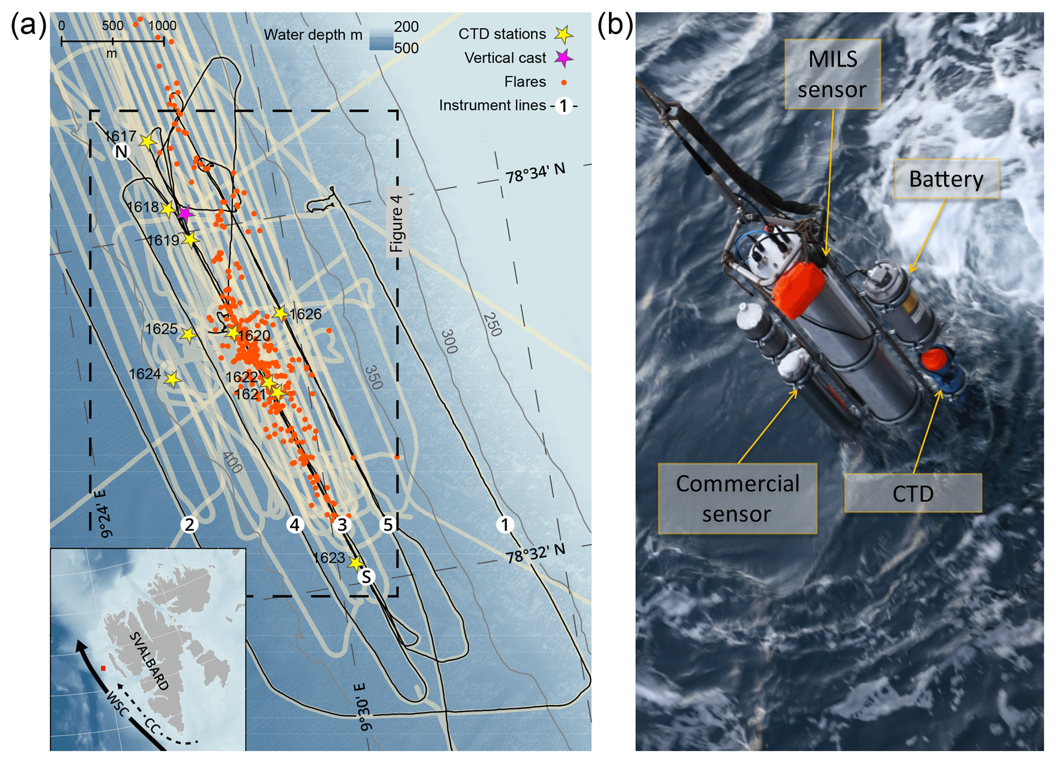
Figure 1Map of the surveyed area and photo of the instrument assembly. (a) Survey lines and sampling locations over the study area at the Svalbard continental margin. Black lines show the ship trajectory with line numbers assigned in the order they were surveyed. Beige areas appearing as thick lines indicate echo-sounder beam coverage from this campaign and previous cruises (AOEM 2010 and CAGE 13-7 in 2013). The start and end locations of line 3 are indicated with N and S, respectively. Known flare locations from this survey and surveys in 2010 and 2013 are marked with orange dots. CTD stations with discrete water sampling are marked with yellow stars and the vertical instrument cast with a purple star. The inset image shows an overview of Svalbard with the survey location indicated with a red square. The controlling currents are shown with solid (WSC) and dashed (coastal current) black lines. The bathymetry was obtained from IBCAO version 3.0 (Jakobsson et al., 2012). (b) Instrument assembly: the main central tube is the prototype MILS sensor. The stainless steel frame acts as a platform and allows for attachment of the instrument battery (top-right side), CTD (blue at the bottom right), and a commercial CH4 sensor and its battery pack (left side).
2.2 Hydrocasts with discrete water sampling
Vertical oceanographic profiles were recorded at 10 stations (Fig. 1a) using a Sea-Bird SBE 911 plus CTD (conductivity, temperature, and depth) mounted on a rosette, which carried twelve 5 L Niskin bottles. In January 2015, the CTD was fitted with new sensors. An SBE 4 conductivity sensor and an SBE 3plus premium CTD temperature sensor, with initial accuracies of ±0.001 ∘C and ±0.3 mS m−1. At 24 Hz sampling, the resolutions are 0.0003 ∘C and 0.04 mS m−1.
The Niskin bottles were closed during the up-casts, collecting seawater at different depths for further dissolved CH4 analysis. Headspace equilibration followed by gas chromatography (GC) analysis was carried out in the laboratory at the Department of Geoscience at UiT, The Arctic University of Norway, using the same technique as Grilli et al. (2018). The resulting headspace mixing ratios (ppmv) were converted to in situ concentrations (nmol L−1) using Henry's solubility law, with coefficients calculated according to Wiesenburg and Guinasso Jr. (1979). The sample dilution from addition of a reaction stopper (1 mL of 1 M NaOH solution replacing 1 mL of each 120 mL sample) and the removal of sample water while introducing headspace gas (5 mL of pure N2 replacing 5 mL of sample water) was accounted for. The overall error for the headspace GC method was 4 %, based on standard deviation of replicates.
2.3 Methodology and technology for high-resolution laser spectrometer CH4 sensing
A stainless steel frame attached to a cable connected to an on-board winch served as a platform to which the MILS (an Aanderaa Seaguard TD262a CTD, a standard commercial CH4 sensor) and a battery pack were mounted. This instrument assembly, hereafter called probe, has a total height of ∼1.8 m, a total weight in air of ∼160 kg, and a negative buoyancy of ∼52 kg. We towed the probe for a total of 28 h, providing unsurpassed high-resolution in situ CH4 measurements with a sampling rate of 1 s−1, together with dissolved oxygen data, as well as pressure, temperature, and salinity. The autonomy of the MILS was ∼12 h at 50 W power consumption. The sensors fitted to the Aanderaa CTD, a conductivity sensor 4319, a temperature sensor 4060, and an oxygen optode 4330, have initial accuracies of ±0.03 ∘C, ±5 mS m−1, and µM and resolutions of 0.001 ∘C, 0.2 mS m−1, and <1 µM, respectively.
Lowering and heaving of the probe in the water column allowed for vertical casts, while towing the probe behind the moving ship at varying heights above the seafloor generated near-horizontal trajectories. The main horizontal trajectories, acquired at a ship speed of 1.5±0.15 knots, comprise five lines (Fig. 1a), where the desired distance from the seafloor was attained by monitoring the pressure in real time while adjusting the cable payout. The battery-powered MILS (Fig. 1b, see Grilli et al., 2018, for more details) has a membrane-inlet system, linked to an optical feedback cavity-enhanced absorption spectrometer, and an integrated PC for control and data storage. Cabled real-time communication with the instruments allowed for instant decision-making and ensuring optimal sensor operation during the deployments.
Sensors with membrane inlets can be sensitive to fluctuating water flow over the membrane, which can result in artificial variability in measured concentrations. The SBE5T pump, which provided a steady water flow of 0.8 L min−1 during all deployments, was positioned about 25 cm away from the membrane inlets and connected with short 1∕2 in. hose sections and a T-piece. By shielding the inlet and outlets and mounting them at the same height with an open flow-path, pressure changes due to movement through the water column were minimized. The water pump inlet has a fine-mesh filter and a shield to avoid entry of free gas bubbles and artefacts from gas bubbles entering the sampling unit and reaching the membrane surface.
All parameters from the MILS sensor, including gas flow, pressure, sample humidity, and internal temperature, were logged to process and evaluate the quality of the data. A dedicated ship-mounted GPS logged positional data for accurate synchronization of the probe and ship position. A position correction, accounting for the lag between the probe and the ship, synchronizes the towed instrument data with simultaneously acquired echo-sounder data. The MATLAB routine “Mooring Design and Dynamics” (Dewey, 1999) simulated the towing scenario for which we used a simplified instrument assembly composed of a cylinder 1.68 m long, 0.28 m in diameter with a negative buoyancy of 52 kg, corresponding to the volume and buoyancy of the whole instrument assembly. A polynomial speed factor () was derived to account for the combined ship and water current velocities (u in metres per second, m s−1). The distances of the probe behind the ship and the corresponding required time shifts were calculated by multiplying the non-dimensional speed factor (x*) with the instrument depth at each data point. This approach allowed for dynamic correction of data positions, accounting for towing with or against the water current, and a near-stationary ship during vertical profiling. Correction for tidal currents was neglected since tides constituted less than 5 % of the WSC of ∼0.2 m s−1 during our deployments, according to the tide model TPXO (Egbert and Erofeeva, 2002).
A time lag of 15 s for the MILS was calculated based on the volume of the gas line between the extraction system and the measurement cell and the gas flow rate (6.5±0.02 cm3 min−1). We expect that concentration profiles obtained from down- and up-casts align when this time lag is applied. The response time of the MILS is given by the flushing time of the measurement cell, and for this campaign the T90 was 15 s.
Mixing ratios of CH4 (ppmv) measured by the MILS were converted into aqueous concentrations (nmol L−1) using Henry's law, where the solubility coefficients were determined according to Wiesenburg and Guinasso Jr. (1979), while accounting for in situ pressure, temperature, and salinity. The uncertainty in the dissolved CH4 measured with the MILS is ±12 % (Grilli et al., 2018).
2.4 Acoustic mapping and quantification of seafloor CH4 emissions
Gas bubbles in the water column are efficient sound scatterers and ship-mounted echo sounders can therefore be used for identifying and quantifying gas emissions (Weber et al., 2014; Veloso et al., 2015; Ostrovsky et al., 2008). The target strength, defined as 10 times the base-10 logarithmic measurements of the frequency-dependent acoustic cross sections (Medwin and Clay, 1997), quantifies the existence of sound scattering objects in the water column. Time series of target strength are displayed in so-called echograms (Greinert et al., 2006; Judd and Hovland, 2009). During the cruise, the 38 kHz channel of the ship-mounted single-beam Simrad EK-60 echo sounder recorded acoustic backscatter continuously. Flares can be identified in the echograms and distinguished from other acoustic scatter from fish schools, dense plankton aggregations, and strong water density gradients. We identify flares as features in echograms, which exceed the background backscatter by more than 10 dB, with a vertical extension larger than their horizontal, and which are attached to the seafloor.
We used the methodology developed and corrected by Veloso et al. (2015, 2019a) and the prescribed FlareHunter software for mapping and quantifying gas release. For the flow rate calculations performed with the Flare Flow Module of FlareHunter, we used a bubble size spectrum with a Gaussian distribution peaking at 3 mm equivalent radius, previously observed in the area (Veloso et al., 2015). Temperature, salinity, pressure, and sound velocities, all required for correct quantification, were provided by the CTD casts. The resulting flow rates and seepage positions allow for mass balance calculation in the control volume model and in the two-dimensional (2-D) model, as described in Sect. 2.5 and 2.6, respectively.
2.5 Control volume model
The temporal evolution (dC∕dt) of a solute's concentration C within a certain volume V, which is fixed in space, and with water flowing through it can, using mass conservation, be written as
Equation (1) is a second-order differential equation from which an analytical steady-state solution can be derived by following these assumptions: the volumetric flow of water in and out of the control volume, QIN and QOUT, are balanced and are given by a steady water current in the x direction across the width (Δy) and height (Δz) of the control volume. The diffusion is kept homogenous and constant by applying a constant diffusion coefficient k. The background concentration CB is fixed in time and space and F represents the persistent flow of the solute (in this case bubble-mediated CH4) into the volume. The CH4 dissolves completely within the volume and the diffusion occurs across the domain (in the y direction). Using the central difference approximation of the second derivative (∇2) in Eq. (1) and the above assumptions yields that the aqueous CH4 within the volume reaches the steady-state concentration:
Finally, by averaging measured CH4 concentration within a defined volume, and assuming that it represents a steady-state concentration, the bubble flow rate is retrieved from Eq. (2).
where represents the measured average concentration and .
The dimensions of the control volume with volume were chosen to match the length of line 3 (Δx=4.5 km), extended 25 m perpendicularly on each side of the line (Δy=50 m), and extended 75 m vertically (Δz=75 m). A graphic describing the control volume is supplied in Fig. S1 in the Supplement.
2.6 Two-dimensional model
In order to gain insight into the physical processes behind the observed CH4 variability, we constructed a two-dimensional 2-D numerical model resolving the evolution of dissolved CH4 in the water column, which results from CH4-bubble emissions, advection with water currents, and diffusion. The model domain was made 400 m high in the z direction, 4.5 km long in the x direction, and oriented along line 3 (Fig. 1a). The navigation data along this line are linearly interpolated to form the basis for a 2 m gridded model domain starting at 78∘34.54′ N, 9∘25.92′ E and ending at 78∘32.1′ N, 9∘30.58′ E as indicated by N and S in Fig. 1a. FlareHunter-derived flow rates within 50 m from line 3 were projected into the model domain and the source of dissolved CH4, mediated by bubbles, was distributed vertically by applying a non-dimensional source function similar to the approach by Jansson et al. (2019a): , where z is the vertical distance from the seafloor in metres. We calculated source distribution functions S(z) by scaling S0(z) with the flare flow rates and distributed the resulting source into current-corrected x∕z nodes with volumes , where m. The model domain comprises 12 extra cells on each side in the y direction in order to avoid fast diffusion out of the domain while the background concentration is held constant. The 2-D model simulated CH4 diffusion and advection with water currents and was run to steady state using different diffusion coefficients, within the range suggested by Sundermeyer and Ledwell (2001). A graphic representation of the 2-D model is shown in Fig. S1.
3.1 Water properties
The measurements from the Sea-Bird CTD during our survey indicate well-mixed water within 150 m above the seafloor and continuously stratified water upwards to 50 m b.s.l. (metres below the sea level) (Fig. 2a) with a squared buoyancy frequency of ∼ N2 < s−2. A pycnocline exists at ∼30 m b.s.l. (Fig. 2a) with N2 up to 10−4 s−2, marking the transition between surface water and AW below (Fig. 2b and c). Temperatures close to the seafloor range from 4.2 to 4.4 ∘C, which is more than 1 ∘C above the CH4 hydrate stability limit (Tishchenko et al., 2005) for a salinity of 35.1 as indicated in Fig. 2a. The velocity of the WSC was between 0.1 and 0.3 m s−1 (Fig. 2d) inferred from the inclination of flare spines (Veloso et al., 2015), which was calculated from the echo-sounder data, obtained throughout the whole survey. The current followed the isobaths, which is consistent with previous findings (Graves et al., 2015; Gentz et al., 2014). The mean salinity and temperature acquired with the Andreaa CTD, in different layers, with their corresponding standard deviations according to the water masses classification by Skogseth et al. (2005) and Ślubowska-Woldengen et al. (2007) are shown in Fig. 2b and c. The temperature and salinity distribution suggests a clear dominance of AW during the survey, overlaid with fresher and colder ASW and PW.
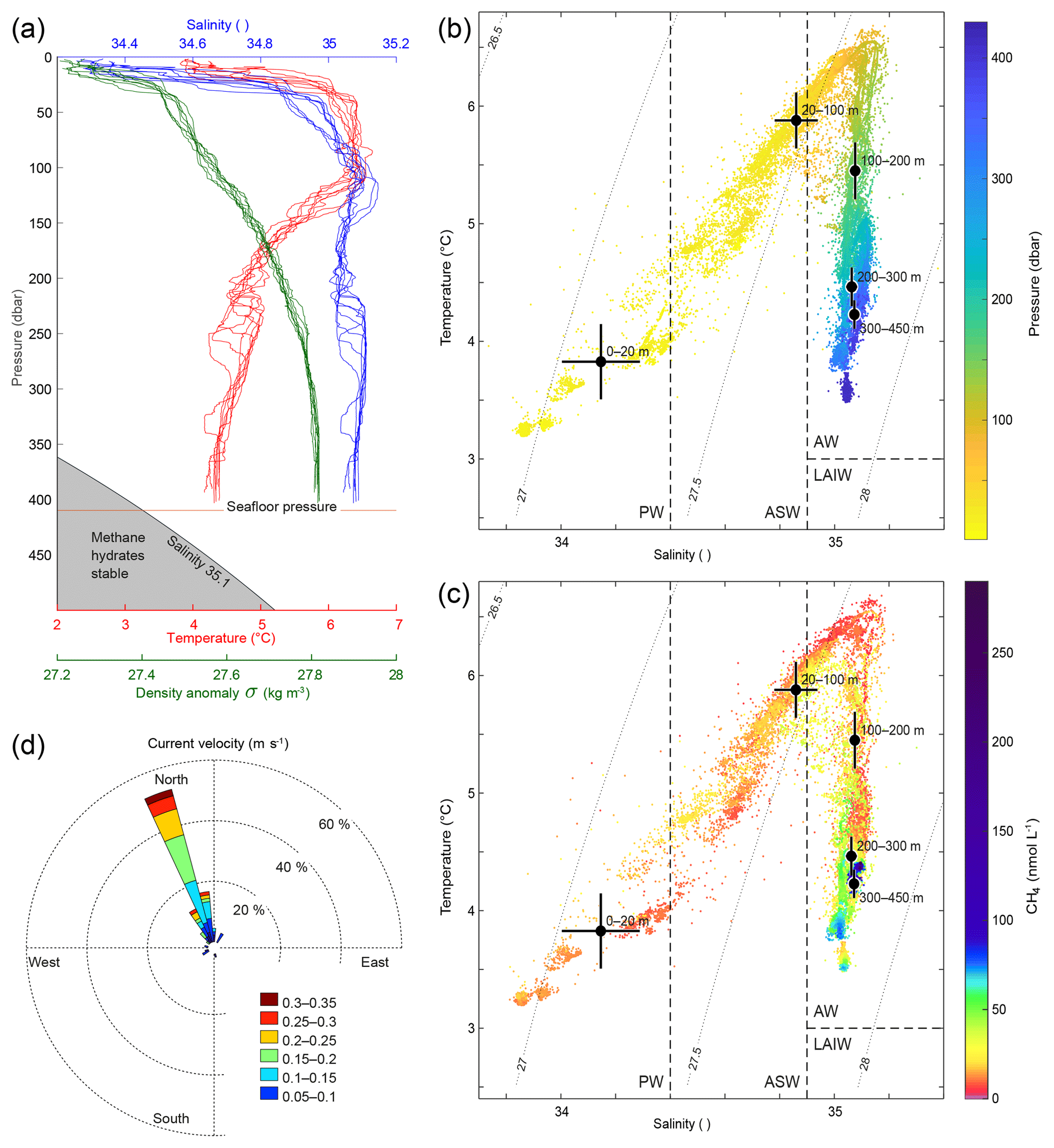
Figure 2Hydrography during the survey. (a) CTD casts 1617–1626 showing temperature (red), salinity (blue), and density anomaly (green) calculated with Gibbs seawater package (McDougall and Barker, 2011). (b) Temperature and salinity diagram coloured by pressure (dbar). Grey curved lines in the background indicate isopycnals (constant density (σ) lines). AW indicates Atlantic Water, PW is Polar Water, ASW is Arctic Surface Water, and LAIW is Lower Arctic Intermediate Water. Water mass definitions are described in the text. Black dots indicate the mean water properties for the different layers and crosses indicate the corresponding standard deviations. (c) Temperature and salinity diagram coloured by CH4 concentrations (nmol L−1) measured with the MILS. Black dots depict average temperature and salinity at water depth intervals and the error bars indicate the corresponding standard deviations. (d) Water currents inferred from inclination of flare spines (Veloso et al., 2015) with a mean bubble rising speed of 23 cm s−1.
3.2 Measured and modelled CH4 distributions
The high-resolution dissolved CH4 concentration profiles resulting from towing the MILS along five lines, approximately 15 m a.s.f. (metres above the seafloor), show high variability (Fig. 3), especially over line 3, which geographically matches the clustering of bubble plumes (Fig. 1a).
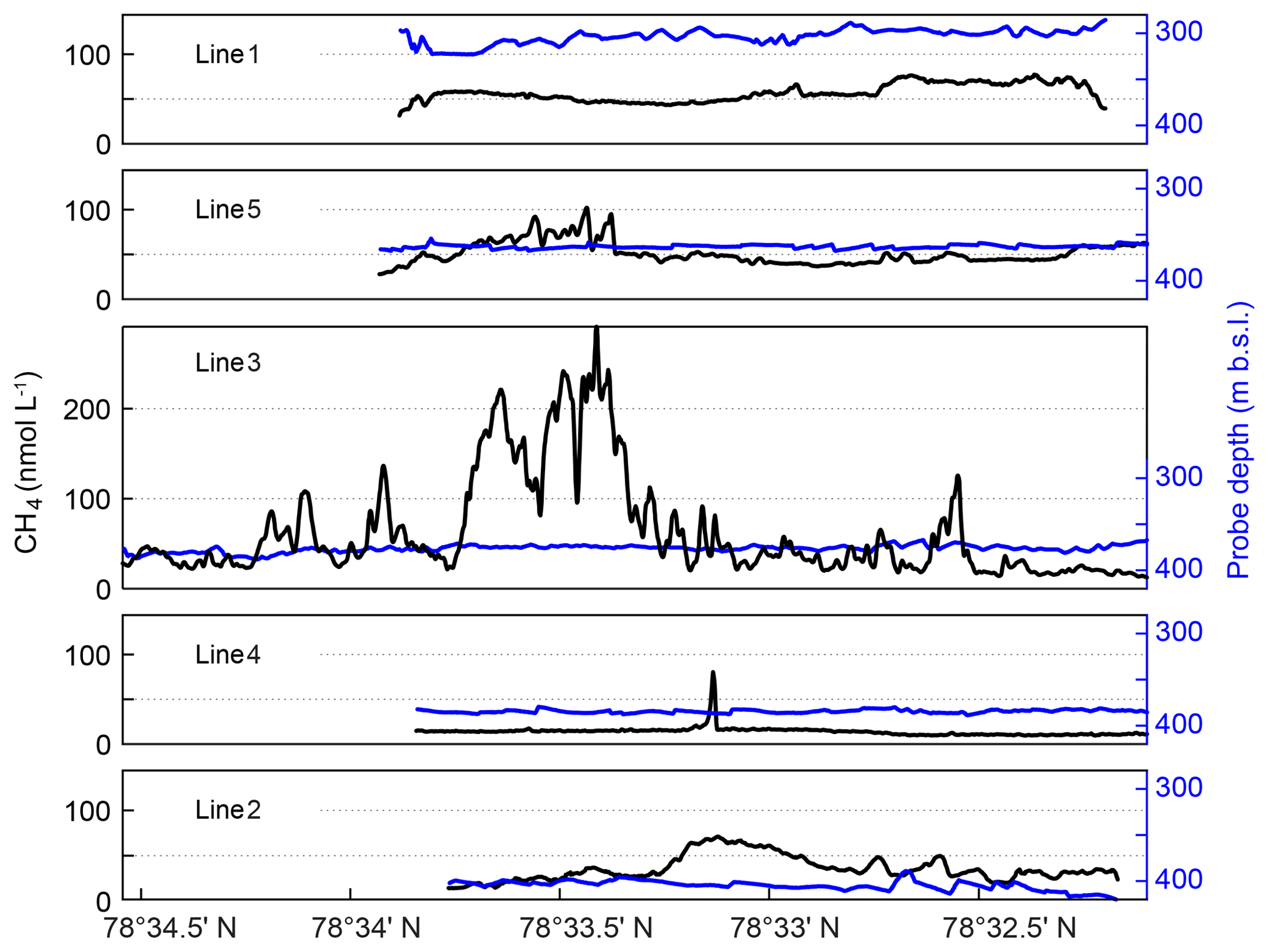
Figure 3MILS measurements along the five lines ∼15 m from the seafloor. Panels show data acquired along lines 1–5, shown in order of proximity to the shore, with line 1 closest to the shore and line 2 furthest offshore. See Fig. 1a for line locations. Black lines show CH4 concentrations, blue lines show the probe depth.
On the landward side (lines 1 and 5), the concentration is relatively smooth with an average of ∼55 nmol L−1 but along line 5, which is closer to the main seepage area, the concentration is influenced by the nearby seepage, inferred from the concentration peaks reaching up to 105 nmol L−1 at 78∘33.5′ N. On the offshore side, the mean concentrations are 15 and 36 nmol L−1 along lines 4 and 2, respectively, with elevated CH4 concentrations of up to ∼70 nmol L−1, lacking hydro-acoustic evidence of CH4 seep sources. The peak in line 4 may be explained by its proximity to the main bubble seep cluster but the CH4 concentrations show more variability along line 2, the most offshore horizontal trajectory of the survey, which may indicate undetected CH4 seepage located deeper than 400 m b.s.l.
A 25 min down- and upward sequence obtained from the vertical MILS cast at station 1616 (Fig. 4) shows excellent repeatability after correcting for the instrument time lag of 15 s. The sensor showed no memory effects, i.e. different response times between increased and decreased CH4 concentrations.
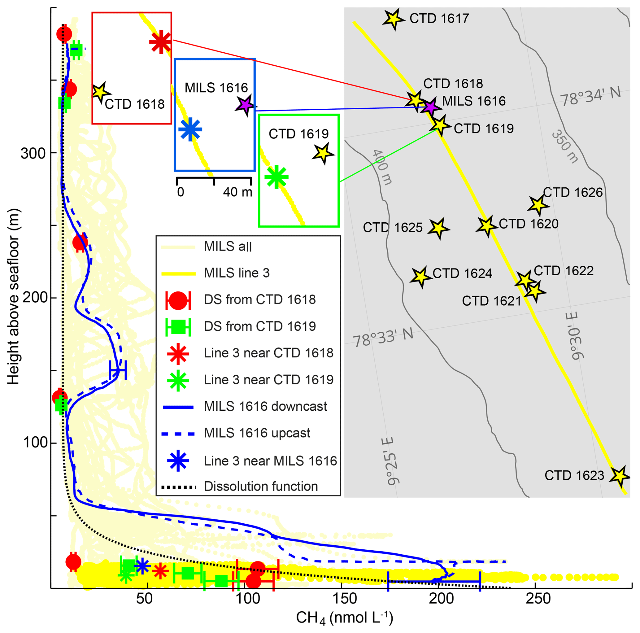
Figure 4High-resolution CH4 concentrations and discrete samples. Light-yellow lines show CH4 concentrations acquired with the MILS during the entire survey and the bright yellow derives from line 3 at ∼15 m a.s.f. only. Solid and dashed blue lines represent continuous down- and upward profiles acquired at station 1616 after correction for instrument response time. The blue error bars indicate the instrument uncertainty of 12 %. Discrete sample data are shown as red dots (CTD 1618) and green squares (CTD 1619) with error bars that indicate the discrete sampling or headspace GC method uncertainty of 4 %. The asterisks indicate MILS data points from the towing along line 3, closest to the vertical cast 1616 (blue), to CTD 1618 (red) and CTD 1619 (green). The dotted black line indicates the exponential dissolution function described in the text. The inset map shows the locations of the CTDs with discrete sampling (station nos. 1617–1623) (yellow stars) as well as line 3, which is indicated with a yellow line. The blue rectangle shows the location of the vertical MILS profile from station 1616 (purple star) and the data point from line 3, which is closest to the deepest location of the vertical cast (blue asterisk). The green rectangle shows the location of CTD 1619 and the closest point on line 3 (green asterisk), while the red rectangle shows the location of CTD 1618 and the corresponding point on line 3 (red asterisk). Bathymetric contours were drawn from the IBCAO dataset (Jakobsson et al., 2012).
Analysis of discrete samples (DSs) from CTD casts 1618 and 1619 and the vertical MILS cast 1616 give further insights into the heterogeneity and temporal variation in the dissolved CH4 distribution (Fig. 4). Discrete measurements from CTDs 1618 and 1619 reveal a qualitative match with the MILS measured concentrations extracted from line 3 near these stations (red and green symbols in Fig. 4). Discrepancies between the MILS cast 1616 and the DS from CTDs 1618 and 1619 close to the seafloor are likely due to the difference in sampling location, as the MILS vertical cast 1616 was ∼150 and ∼180 m away from CTDs 1618 and 1619, respectively.
The exponential “dissolution” function, which represents the expected trace of dissolved CH4 in the water column, resulting from bubble dissolution, was compared to the entire MILS dataset by plotting CH4 concentrations against height above the seafloor, determined from position-corrected pressure and previously acquired multibeam data (Fig. 4).
Elevated CH4 concentrations at ∼160 and ∼220 m b.s.l. revealed by the MILS vertical profile 1616 were not identified with DSs from the nearby CTD cast 1619, and DSs from CTD 1618 reveal only a small fraction of the CH4 anomaly because of sampling that is too sparse (Fig. 4). The MILS data collected 15 m a.s.f. along line 3 reveal 50 nmol CH4 L−1 while the vertical profile only 30 metres away (MILS-cast 1616) measured ∼200 nmol CH4 L−1 (Fig. 4). This emphasizes the strong spatio-temporal variability in the CH4 distribution in the area.
Despite the high CH4 variability in the horizontal profiles (Fig. 3), further analysis of the data may be obtained by focusing on line 3, towed in a north–south direction at ∼0.8 m s−1 directly over the bubble streams. Based on a mean depth of 390 m and the depth of the towed CTD, the height above the seafloor of the towed probe along line 3 was 13.4±3.8 m. The fast response time of the MILS sensor (T90=15 s) revealed decametre-scale variations in the dissolved CH4 concentrations with high values well correlated with the echo-sounder signal, after correcting for the towed instrument position (Fig. 5).
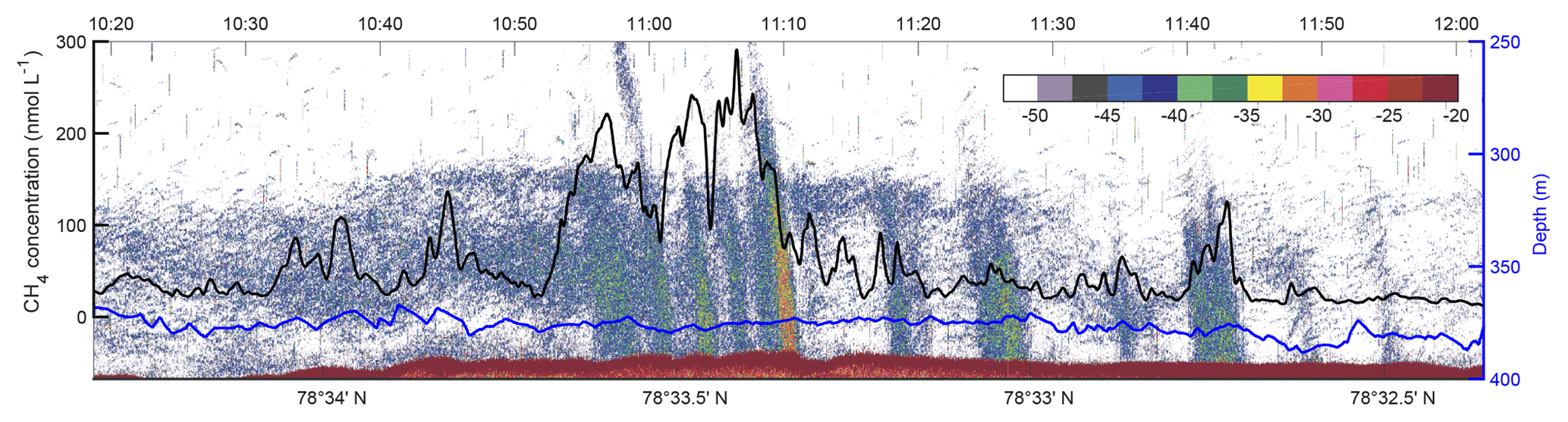
Figure 5Towed MILS data overlying echo-sounder data. The black line shows the CH4 concentration along line 3 (see Fig. 1 for location) at ∼15 m from the seafloor. The blue line indicates the depth of the probe. The echogram, displaying target strength values (colour bar shows intensity – dB) from the 38 kHz channel of the EK60, is shown in the background.
A close analysis of the measured concentration reveals that the up- and downstream gradients are equally distributed (bar chart in Fig. S2c). This symmetry suggests that CH4 disperses fast and equally in all horizontal directions around the bubble plumes while being advected away from the source.
The measured CH4 concentrations along line 3 changed significantly (5 % or more) on sub-response times (<15 s) in only two instances and over a total time of 26 s, out of 1 h 42 min, as indicated with red dots in Fig. S2a. This suggests that the MILS resolved 99.6 % of the gradients and that the response time of the MILS did not limit the resolution of the CH4 distribution. The mean absolute gradient, assessed from steadily increasing or decreasing concentrations (vertical grey lines in Fig. S2a show the position of the selected slopes), was 1.5 nmol L−1 m−1, corresponding to 1.2 nmol L−1 s−1. The minimum and maximum lateral gradients were −5.0 and 4.8 nmol L−1 m−1, respectively, which correspond to −4.1 and 4.6 nmol L−1 s−1. Correlations of CH4 concentrations versus depth and speed changes were low (R=0.0133, −0.0001, −0.0094, and 0.0028 for ship speed, ship acceleration, vertical instrument speed, and instrument acceleration, respectively), showing the stability of the instrument during rapid movements and disproving artefacts due to water flow fluctuations at the membrane.
Sources of CH4 constraining the control volume and 2-D model were obtained from the acoustic mapping and quantification described in Sect. 2.4. During the entire survey, we identified 68 unique groups of bubble plumes, with an average flow rate of 48 (SD = 50) mL min−1. Within 50 m of line 3, we acoustically identified 31 flares with an average flow rate of 60 (SD = 65) mL min−1 amounting to a total flow rate of 1.87 L min−1. These flow rates were taken as sources in the control volume and 2-D model. FlareHunter calculates the flow rates in a layer 5–10 m above the seafloor. In order to calculate flow rates from the seafloor, we upscaled the FlareHunter flow rates by 40 % to compensate for bubble dissolution near the seafloor, in accordance with the dissolution profile.
The 2-D model was run to steady state with different diffusion coefficients, k∈[0.3–4.9 m2 s−1], adopted from dye experiments offshore Rhode Island (Sundermeyer and Ledwell, 2001). These coefficients are in agreement with the ones obtained from the Celtic Sea (k∈[0.8–4.4 m2 s−1]) (Stashchuk et al., 2014) but much higher than the coefficient applied by Graves et al. (2015) (k=0.07 m2 s−1). The best fit between the 2-D model and the MILS data (R=0.68) was achieved during a simulation with k=1.5 m2 s−1. Because the high-end coefficients of Sundermeyer and Ledwell (2001) and Stashchuk et al. (2014) were derived during wavy conditions, and because our model mainly resolves the near-bottom region away from wave action, we interpret that our best-fit diffusion coefficient is relatively high. The resulting range of model outputs and the best-fit model simulation are visualized and compared with high-resolution measurements in Fig. 6. Despite applying a high diffusion coefficient, the 2-D model shows a residual downstream tailing which is not seen in the MILS data. We attribute this to the fact that the model does not resolve small-scale eddies, but only diffusion across the domain and diffusion and advection along the domain.
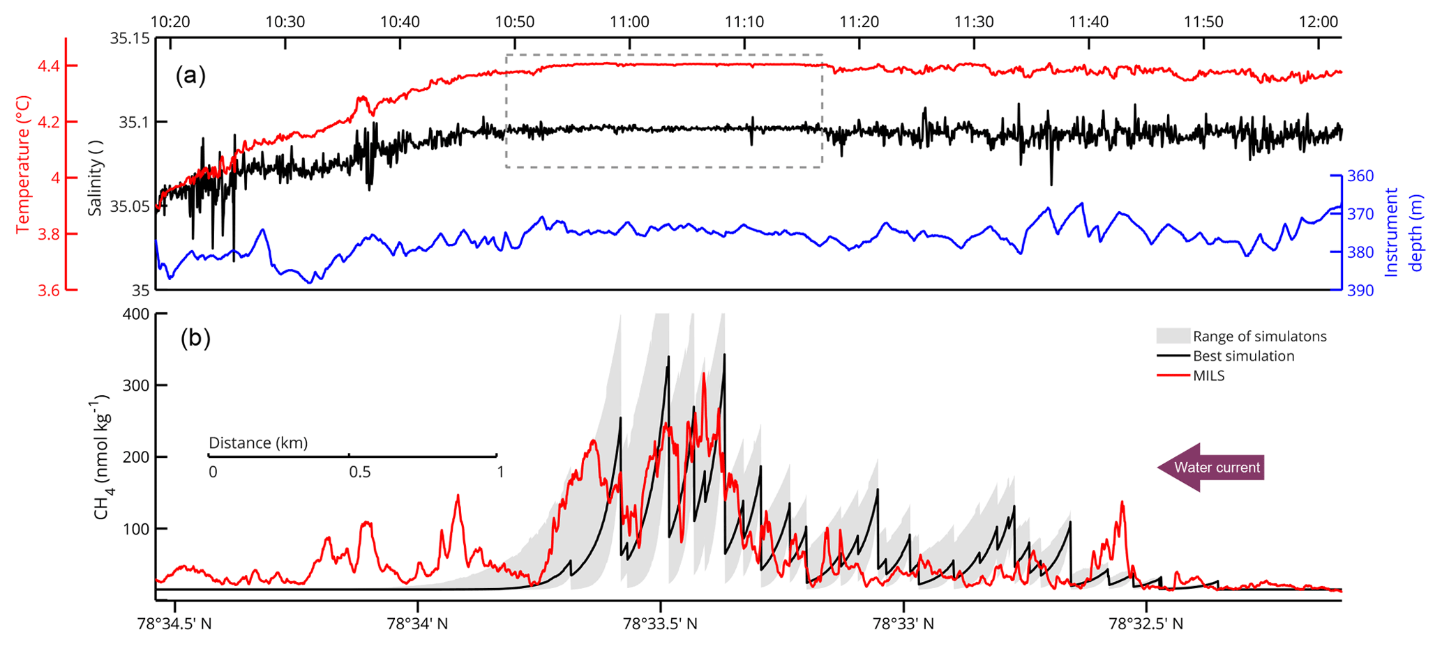
Figure 6Water properties and comparison between modelled and measured dissolved CH4 concentrations along line 3. (a) Shows temperature and salinity data together with the depth of the towed instruments. The dashed-line box highlights the area of intense mixing. In (b), the red line shows the dissolved CH4 measured by the MILS. The grey area indicates the range of CH4 concentrations from the 2-D model simulations. The black line depicts output of the model simulation with the best match with the measured concentrations.
The salinity and temperature profiles of the towed CTD indicate well-mixed water, particularly over the most prominent gas flares. Here, the relative standard deviation of the salinity and temperature drops by factors of 10 and 58, respectively, as highlighted by the dashed-line box in Fig. 6. The depth stability of the probe is also better in the area. Its relative standard deviation dropped by a factor of 3, which is not enough to justify the larger factors observed for the temperature and salinity. We interpret that this is caused by turbulent mixing enhanced by the bubble streams.
3.3 Methane inventory
The method, dimensions, and resolution chosen for calculating CH4 inventories may strongly influence the resulting content and average concentrations. This may have serious implications when the results are used for upscaling. To highlight this, we applied different inventory calculation methods on the same water volume.
Averages along line 3 were calculated from the following: (a) concentrations from discrete sampling, based on different sampling depths; (b) discrete data from different depths, linearly interpolated along the line; (c) high-resolution data obtained from the MILS data ∼ 15 m a.s.f.; and (d) concentrations extracted from the 2-D model output at steady state at 15 m a.s.f.
Average concentrations were calculated in a box volume equivalent to MILS line 3: 4.5 km long (x direction), 50 m wide (y direction), which is equivalent to the echo-sounder beam width 75 m high (z direction), which corresponds to the most dynamic and CH4-enriched zone (e.g. McGinnis et al., 2006; Jansson et al., 2019a; Graves et al., 2015). Box averages were derived as follows. The volume was divided into 1 m cubic cells. Cells located in the y centre and in z positions vertically matching the underlying data (DS or MILS) were populated with the MILS or interpolated DS profiles. The remaining cells were populated by perpendicular and vertical extrapolation following the typical horizontal gradient of 1.5 nmol L−1 m−1 and vertical dissolution profiles scaled by the measured or interpolated concentrations. The mean concentrations from the 2-D model were delimited by the height of the box. The control volume model provided only one value for the entire box.
The underlying data and their interpolation is seen in Fig. 7 and the resulting averages are reported in Table 1.
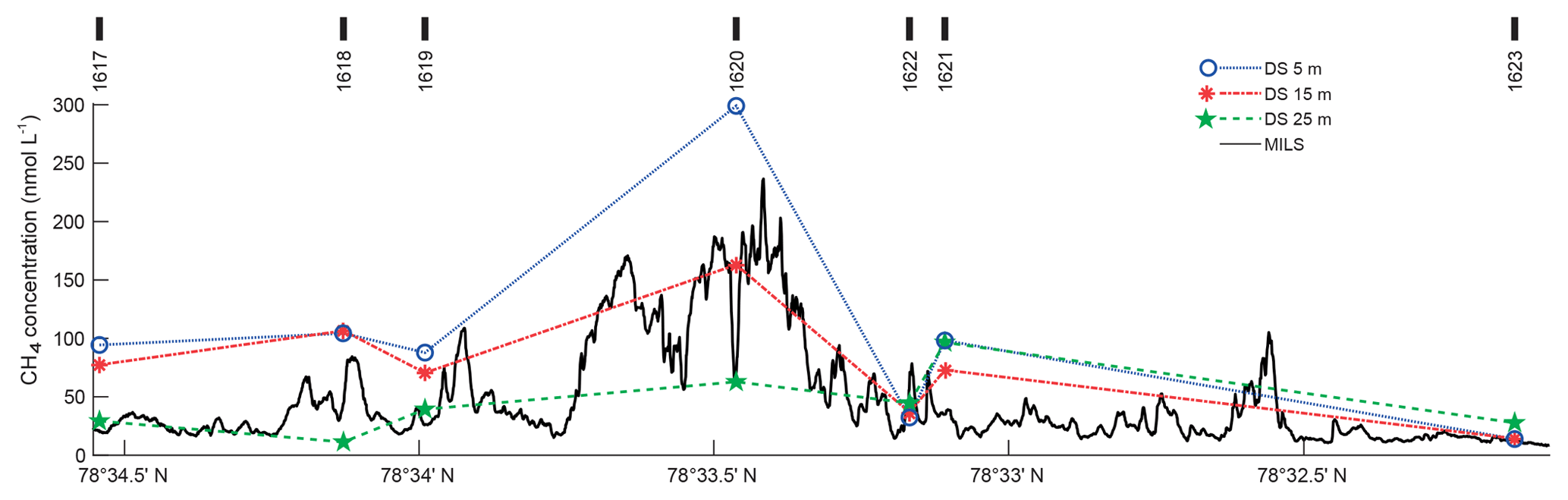
Figure 7Underlying CH4 concentration data for inventory calculations. Solid black line shows the continuous MILS profile ∼15 m a.s.f. along line 3. DS concentrations at various depths are shown as blue circles, red asterisks, and green stars for 5, 15, and 25 m a.s.f., respectively, and blue dotted, red dash-dotted, and green dashed lines represent the corresponding linear horizontal interpolations. CTD cast numbers are marked with thick black lines at the top of the graph.
Table 1Average concentrations (nmol L−1) calculated with different methods at different altitudes as indicated in the first column (metres above the seafloor, m a.s.f.). 1 Average of the sparse discrete sampling from CTD casts 1617–1623. 2 Average of high-resolution (MILS) measurements from line 3. 3 Average of linearly interpolated concentrations based on discrete measurements (CTDs 1617–1623). 4 Average concentrations from the 2-D model, extracted from depths matching the MILS position along line 3. 5 Average concentrations within the box (4500 m (L) × 50 m (W) × 75 m (H)) based on the high-resolution measurements or interpolated concentrations along the box, vertical distribution based on the dissolution profile, and horizontal distribution across the width of the box based on the mean horizontal concentration gradient (Fig. S2). 6 Average of the 2-D model (best simulation) result from 0 to 75 m a.s.f. and across the domain. 7 The control volume (CV) model yields a box value only.
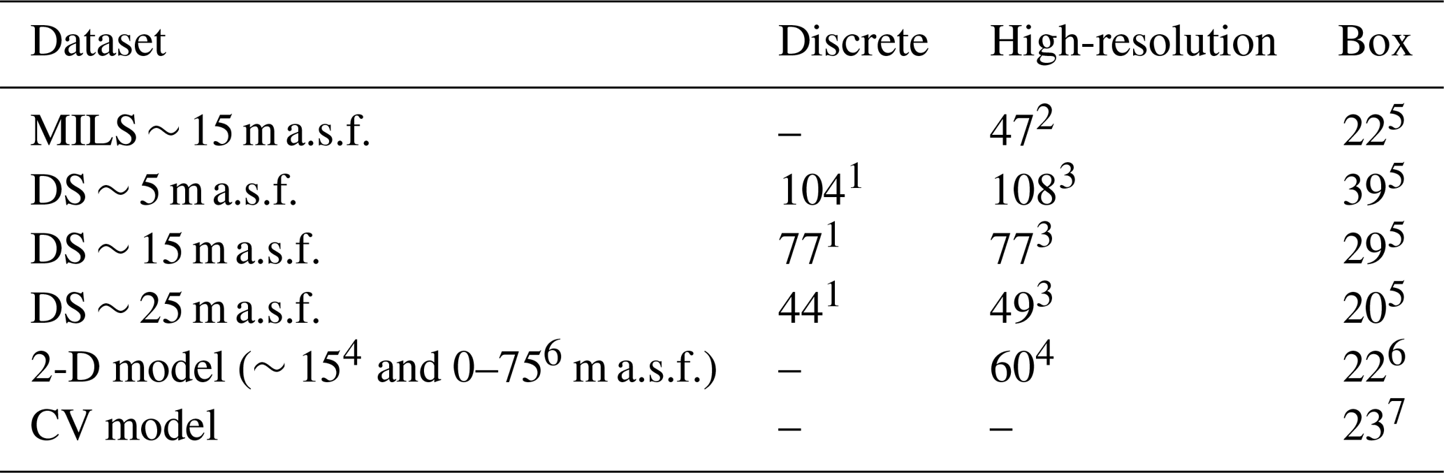
The average CH4 concentration in the box volume based on continuous data is similar to the average obtained from discrete data at 15 m above the seafloor. We obtained 47 nmol L−1 vs. 77 nmol L−1 for the high-resolution line and the interpolated DS, while the box averages for the high-resolution and interpolated DS were 22 nmol L−1 vs. 29 nmol L−1. The 2-D model yielded a line average of 60 nmol L−1, while it was 22 nmol L−1 for the box. The control volume model predicted a steady-state concentration of 23 nmol L−1 when the diffusion coefficient was 1.5 m2 s−1, inferred from the 2-D model applied.
During our survey, the mean flow rate at the seafloor per flare within 50 m of line 3 was 84 (SD = 91.6) mL min−1, (min = 15.8, max = 355.6 mL min−1). This is comparable with the flow rate per flare of 125 mL min−1 estimated by Sahling et al. (2014), who assumed that an acoustic flare consists of six bubble streams, each with a flow rate of 20.9 mL min−1. The authors found 452 flares in the area for which they assumed similar flow rates and thereby calculated a total flow in the area of ∼57 L min−1. Our study encompasses a smaller area, where we only detected 68 flares (31 flares within 50 m of line 3) and the total flow rate from these 68 flares was 4.56 L min−1. This total flow translates to 65.7 t CH4 yr−1 assuming constant ebullition. Considering the sparse beam coverage and relatively small area, this may be compared to CH4 seepage of ∼550 t CH4 yr−1 estimated for a larger area, covered by nine surveys (Veloso et al., 2019b), and ∼400 t CH4 yr−1 (Sahling et al., 2014), in a study area covering ours but also extending northwards where additional gas venting occurs. A comparison of studies from the same area, using different methods, shows a large range of yearly CH4 emissions to the water column. Flow rates of CH4 per distance along the continental shelf from previous studies given by the authors, 900 kg m−1 yr−1 (Westbrook et al., 2009); 141 kg m−1 yr−1 (Reagan et al., 2011); 13.8 (6.9–20.6) t m−1 yr−1 (Marín-Moreno et al., 2013); 2400 (400–4500) mol m−1 yr−1 (Sahling et al., 2014); and 748 (561–935) t m−1 yr−1 (Berndt et al., 2014), yield emissions of 4050, 635, 992, 173 and 54 000 t CH4 yr−1, respectively, over the 4500 m section of the continental shelf which corresponds to our line 3.
The MILS data collected 15 m a.s.f. along line 3 do not reveal the high concentrations (∼200 nmol L−1) measured during the vertical cast only 30 m away, emphasizing the heterogeneous CH4 distribution and highlighting the need for high-resolution sensing rather than sparse discrete sampling.
The fast response of the MILS helped reveal decametre-scale variability in dissolved CH4 and we conclude that uncertainties introduced by MILS response time were negligible in this survey. The observed symmetry of CH4 gradients suggests fast dispersion in all horizontal directions while enriched water is advected away from the sources.
Because the instrument assembly lacked an inertia measurement unit, the stability during towing is unknown but we did not observe any effect on the measurements from wobble and/or rotation.
Gentz et al. (2014) and Myhre et al. (2016) suggested that a pronounced pycnocline is a prerequisite to limit the vertical transport of dissolved CH4 towards the surface. One should note that this hypothesis is based on discrete sample data rather than high-resolution data. We observed high CH4 concentrations up to 75–100 m a.s.f., which is in agreement with bubble models (e.g. McGinnis et al., 2006; Jansson et al., 2019a), highlighting that bubbles of observed sizes (∼3 mm average equivalent radius) are fully dissolved within this range. Density stratification plays an important role in the vertical distribution of dissolved CH4 because turbulent energy is required to mix solvents across isopycnals. Vertical mixing is therefore inhibited even without the presence of a strong pycnocline. We suggest that the observed height limit is a result of rapid bubble dissolution and inefficient vertical mixing, regardless of the existence of a pronounced pycnocline.
We observed CH4 concentrations of up to 100 nmol L−1 without the acoustic signature of flares north of the active flare zone (Fig. 5). Echograms from the CAGE 15-6 survey (this work) and previous surveys conducted in 2010 (AOEM 2010 cruise, University of Tromsø, with R/V Jan Mayen) and 2013 – CAGE 13-7 cruise, with R/V Helmer Hanssen (e.g. Portnov et al., 2016) – reveal that the nearest bubble stream is located ∼300 m northeast of this CH4 anomaly. Several hypotheses may explain this CH4 enrichment: (a) nearby presence of CH4-enriched water seepage (hypothetically from dissociating hydrates) from the seafloor; (b) presence of bubble streams with bubbles too small to be detected by the echo sounder (the detection limit (target strength < −60 dB) of a single bubble was 0.42 mm for this survey); and (c) advection of CH4-enriched water from an upstream bubble plume source, not detected by the echo sounder. In our case, the temperature- and salinity anomaly, which coincides with the increased CH4, reveals mixing of AW with colder and fresher water (Fig. 6). Because mixing lines drawn in the temperature and salinity diagrams (Fig. 2b and c) point towards PW rather than a pure fresh water source, our data support hypothesis (c), namely that AW mixed with PW was transported and enriched in CH4 while passing over a bubble plume before reaching the location of the measurement. Lateral eddies or bottom Ekman transport may have been responsible for the intrusion of fresh, cold, CH4-enriched water.
The 2-D model relies on acoustically detected bubble plume locations and the difference between measured and modelled CH4 is obvious along line 3 from 10:30 to 10:50 LT (local time) as seen in Fig. 6. The CH4 signal from high-resolution data, not thoroughly resolved by the model, underscores that mapping and modelling based on echo-sounder data are not enough for a correct quantitative estimate of the CH4 inventory. The 2-D model required a high diffusion coefficient in order to reproduce the variability in measurements, which is supported by high turbulence in the area caused by the strong currents. Downstream tailing of CH4 concentrations seen in the 2-D model was not observed with the MILS. In fact, MILS data reveal an equal distribution of down- and upstream concentration gradients. We explain the discrepancy by the fact that the 2-D model does not resolve eddies and the CH4 source is placed in discrete cells, following a theoretical straight bubble line, and not accounting for diffusion along the bubble paths.
The relatively high midwater (120–260 m b.s.l.) CH4 concentrations revealed by the vertical MILS cast 1616 was only partly observed in the discrete sampling and was not inferred from echo-sounding. We suggest that this discrepancy is attributed to seepages at the corresponding depth interval not previously mapped. The closest known seepages are a few kilometres away from the location at the shallow shelf (50–150 m b.s.l.) and at the shelf break (∼250 m b.s.l.) (Veloso et al., 2015), but it is doubtful that water masses from these locations can reach the surveyed area as the WSC is persistently northbound. Unless horizontal eddies transport CH4 from the shelf break to this area, this result indicates the existence of undiscovered CH4 bubble plumes further south at the depth of the observed anomaly.
The high-resolution data from the MILS result in a significantly lower CH4 inventory than the one obtained from discrete sampling (47 nmol L−1 vs. 77 nmol L−1) due to the heterogeneous distribution of dissolved CH4. The choice of discrete sample locations can significantly affect the resulting average concentration. The average CH4 concentration (93 nmol L−1) estimated by Graves et al. (2015) from a box with dimensions Δx=1 m, Δy=50 m, and Δz=75 m, obtained from a DS transect across the slope, was substantially higher than our box estimates of 20–39 nmol L−1. These two results highlight the need for high-resolution sensing when estimating CH4 inventories and average CH4 concentrations.
The optical spectrometer of the MILS can be tuned or replaced to improve its sensitivity or to sample more CH4-enriched waters. We believe the MILS would be an excellent tool for evaluating CH4-related water column processes. Grilli et al. (2018) reported a sensitivity of ±25 ppbv in air which translates to ±0.03 nmol L−1 at 20 ∘C and a salinity of 38, which is low enough for investigations of atmospheric exchange and CH4 production or consumption rates.
We have presented new methods for understanding the dynamics of CH4 after its release from the seafloor, coupling for the first time continuous high-resolution measurements from a reliable and fast CH4 sensor (MILS) with dedicated models. The MILS sensor was successfully deployed as a towed body from a research vessel and provided high-resolution real-time data of both vertical and horizontal dissolved CH4 distribution in an area of intense seepage west of Svalbard. For the first time, we observed a more heterogeneous CH4 distribution than has been previously presumed.
We employed an inverse acoustic model for CH4 seepage mapping and quantification which provided the basis for a new 2-D model and a new control volume model, which both agreed relatively well with observations. The 2-D model did not reproduce the symmetric gradients observed with the MILS, which suggests a need to improve the model by including turbulent mixing enhanced by the bubble streams.
Despite the large spatial and temporal variability in the CH4 concentrations, a comparison between high-resolution (MILS) and DS data showed good general agreement between the two methods.
Heterogeneous CH4 distribution measured by MILS matched acoustic backscatter, except for an area with high CH4 concentrations without acoustic evidence of CH4 source. Similarly, high midwater CH4 concentrations were observed by the MILS vertical casts with little evidence of a nearby CH4 source, further supporting that high-resolution sensing is an essential tool for accurate CH4 inventory assessment and that high-resolution sensing can give clues to undetected sources.
CH4 inventories, given by discrete sampling, agreed with those from high-resolution measurements but sparse sampling may over- or underestimate inventories, which may have repercussions if the acquired data are used for predicting degassing of CH4 to the atmosphere in climate models. The added detail of the fine structure allows for better inventories, elucidates the heterogeneity of the dissolved gas, and provides a better insight into the physical processes that influence the CH4 distribution.
The methods for understanding CH4 seepage presented here show potential for improved detection and quantification of dissolved gases in oceans and lakes. Applications for high-resolution CH4 sensing with the MILS include environmental and climate studies as well as gas leakage detection desired by the fossil fuel industry.
A dataset comprising the MILS sensor data and echo-sounder files is available from the UiT Open Research Data repository https://doi.org/10.18710/UWP6LL (Jansson et al., 2019b).
The supplement related to this article is available online at: https://doi.org/10.5194/os-15-1055-2019-supplement.
PJ and JT contributed equally to the work leading to this article, and are listed alphabetically. JM and JC initiated the collaboration and designed the study. JT, RG, PJ, and JM planned and participated in the field campaign. JT and RG systematized and synchronized the high-resolution MILS data. PJ mapped and quantified gas seepage and water currents by collecting and analysing echo-sounder data. PJ collected and analysed the CTD data and water samples and organized the data repository. RG converted mixing ratios to aqueous concentrations. PJ developed the numerical models. AS analysed the water mass properties. JT and PJ calculated CH4 inventories. All authors contributed to the article.
The authors declare that they have no conflict of interest.
We thank the crew on board R/V Helmer Hanssen for the assistance during the cruise and the University of Svalbard for the logistics support. We also thank three anonymous referees for their suggestions to improve this article.
The research leading to these results has received funding from the European Commission's Seventh Framework Programmes ERC-2011-AdG under grant agreement no. 291062 (ERC ICE & LASERS), as well as ERC-2015-PoC under grant agreement no. 713619 (ERC OCEAN-IDs). Additional funding support was provided by SATT Linksium of Grenoble, France (maturation project SubOcean CM2015/07/18). The collaboration between CAGE and IGE was initiated thanks to the European COST Action ES902 PERGAMON. The research is part of the Centre for Arctic Gas Hydrate, Environment and Climate (CAGE) and is supported by The Research Council of Norway through its Centres of Excellence funding scheme grant no. 223259.
This paper was edited by Mario Hoppema and reviewed by three anonymous referees.
Andreassen, K., Hubbard, A., Winsborrow, M., Patton, H., Vadakkepuliyambatta, S., Plaza-Faverola, A., Gudlaugsson, E., Serov, P., Deryabin, A., Mattingsdal, R., Mienert, J., and Bünz, S.: Massive blow-out craters formed by hydrate-controlled methane expulsion from the Arctic seafloor, Science, 356, 948–953, https://doi.org/10.1126/science.aal4500, 2017.
Berndt, C., Feseker, T., Treude, T., Krastel, S., Liebetrau, V., Niemann, H., Bertics, V. J., Dumke, I., Dünnbier, K., Ferré, B., Graves, C., Gross, F., Hissmann, K., Hühnerbach, V., Krause, S., Lieser, K., Schauer, J., and Steinle, L.: Temporal Constraints on Hydrate-Controlled Methane Seepage off Svalbard, Science, 343, 284–287, https://doi.org/10.1126/science.1246298, 2014.
Biastoch, A., Treude, T., Rüpke, L. H., Riebesell, U., Roth, C., Burwicz, E. B., Park, W., Latif, M., Böning, C. W., and Madec, G.: Rising Arctic Ocean temperatures cause gas hydrate destabilization and ocean acidification, Geophys. Res. Lett., 38, L08602, https://doi.org/10.1029/2011GL047222, 2011.
Boetius, A. and Wenzhöfer, F.: Seafloor oxygen consumption fuelled by methane from cold seeps, Nat. Geosci., 6, 725–734, https://doi.org/10.1038/ngeo1926, 2013.
Boulart, C., Prien, R., Chavagnac, V., and Dutasta, J.-P.: Sensing Dissolved Methane in Aquatic Environments: An Experiment in the Central Baltic Sea Using Surface Plasmon Resonance, Environ. Sci. Technol., 47, 8582–8590, https://doi.org/10.1021/es4011916, 2013.
Boulart, C., Briais, A., Chavagnac, V., Révillon, S., Ceuleneer, G., Donval, J.-P., Guyader, V., Barrere, F., Ferreira, N., Hanan, B., Hémond, C., Macleod, S., Maia, M., Maillard, A., Merkuryev, S., Park, S.-H., Ruellan, E., Schohn, A., Watson, S., and Yang, Y.-S.: Contrasted hydrothermal activity along the South-East Indian Ridge (130∘ E–140∘ E): From crustal to ultramafic circulation, Geochem. Geophy. Geosy., 18, 2446–2458, https://doi.org/10.1002/2016GC006683, 2017.
Damm, E., Mackensen, A., Budéus, G., Faber, E., and Hanfland, C.: Pathways of methane in seawater: Plume spreading in an Arctic shelf environment (SW-Spitsbergen), Cont. Shelf Res., 25, 1453–1472, https://doi.org/10.1016/j.csr.2005.03.003, 2005.
Dewey, R. K.: Mooring Design & Dynamics – a Matlab® package for designing and analyzing oceanographic moorings, Mar. Models, 1, 103–157, https://doi.org/10.1016/S1369-9350(00)00002-X, 1999.
Egbert, G. D. and Erofeeva, S. Y.: Efficient Inverse Modeling of Barotropic Ocean Tides, J. Atmos. Ocean. Tech., 19, 183–204, https://doi.org/10.1175/1520-0426(2002)019<0183:EIMOBO>2.0.CO;2, 2002.
Ferré, B., Mienert, J., and Feseker, T.: Ocean temperature variability for the past 60 years on the Norwegian-Svalbard margin influences gas hydrate stability on human time scales, J. Geophys. Res.-Oceans, 117, C10017, https://doi.org/10.1029/2012JC008300 2012.
Gentz, T., Damm, E., Schneider von Deimling, J., Mau, S., McGinnis, D. F., and Schlüter, M.: A water column study of methane around gas flares located at the West Spitsbergen continental margin, Cont. Shelf Res., 72, 107–118, https://doi.org/10.1016/j.csr.2013.07.013, 2014.
Graves, C. A., Steinle, L., Rehder, G., Niemann, H., Connelly, D. P., Lowry, D., Fisher, R. E., Stott, A. W., Sahling, H., and James, R. H.: Fluxes and fate of dissolved methane released at the seafloor at the landward limit of the gas hydrate stability zone offshore western Svalbard, J. Geophys. Res.-Oceans, 120, 6185–6201, https://doi.org/10.1002/2015JC011084, 2015.
Greinert, J., Artemov, Y., Egorov, V., De Batist, M., and McGinnis, D.: 1300-m-high rising bubbles from mud volcanoes at 2080 m in the Black Sea: Hydroacoustic characteristics and temporal variability, Earth Planet. Sc. Lett., 244, 1–15, https://doi.org/10.1016/j.epsl.2006.02.011, 2006.
Grilli, R., Triest, J., Chappellaz, J., Calzas, M., Desbois, T., Jansson, P., Guillerm, C., Ferré, B., Lechevallier, L., Ledoux, V., and Romanini, D.: Sub-Ocean: Subsea Dissolved Methane Measurements Using an Embedded Laser Spectrometer Technology, Environ. Sci. Technol., 52, 10543–10551, https://doi.org/10.1021/acs.est.7b06171, 2018.
Hong, W. L., Torres, M. E., Portnov, A., Waage, M., Haley, B., and Lepland, A.: Variations in Gas and Water Pulses at an Arctic Seep: Fluid Sources and Methane Transport, Geophys. Res. Lett., 45, 4153–4162, https://doi.org/10.1029/2018GL077309, 2018.
Jakobsson, M., Mayer, L., Coakley, B., Dowdeswell, J. A., Forbes, S., Fridman, B., Hodnesdal, H., Noormets, R., Pedersen, R., Rebesco, M., Schenke, H. W., Zarayskaya, Y., Accettella, D., Armstrong, A., Anderson, R. M., Bienhoff, P., Camerlenghi, A., Church, I., Edwards, M., Gardner, J. V., Hall, J. K., Hell, B., Hestvik, O., Kristoffersen, Y., Marcussen, C., Mohammad, R., Mosher, D., Nghiem, S. V., Pedrosa, M. T., Travaglini, P. G., and Weatherall, P.: The International Bathymetric Chart of the Arctic Ocean (IBCAO) Version 3.0, Geophys. Res. Lett., 39, L12609, https://doi.org/10.1029/2012gl052219, 2012.
Jansson, P., Ferré, B., Silyakova, A., Dølven, K. O., and Omstedt, A.: A new numerical model for understanding free and dissolved gas progression toward the atmosphere in aquatic methane seepage systems, Limnol. Oceanogr.: Meth., 17, 223–239, https://doi.org/10.1002/lom3.10307, 2019a.
Jansson, P., Triest, J., Grilli, R., Ferré, B., Silyakova, A., Mienert, J., Chappellaz, J.: Replication Data for: High-resolution underwater laser spectrometer sensing provides new insights into methane distribution at an Arctic seepage site, UiT, The Arctic University of Norway, DataverseNO, https://doi.org/10.18710/UWP6LL, 2019b.
Jørgensen, N. O., Laier, T., Buchardt, B., and Cederberg, T.: Shallow hydrocarbon gas in the nothern Jutland-Kattegat region, Denmark, Bull. Geol. Soc., 38, 69–76, 1990.
Judd, A. and Hovland, M.: Seabed fluid flow: the impact on geology, biology and the marine environment, Cambridge University Press, Cambridge, 2009.
Loeng, H.: Features of the physical oceanographic conditions of the Barents Sea, Polar Res., 10, 5–18, https://doi.org/10.3402/polar.v10i1.6723, 1991.
Marín-Moreno, H., Minshull Timothy, A., Westbrook Graham, K., Sinha, B., and Sarkar, S.: The response of methane hydrate beneath the seabed offshore Svalbard to ocean warming during the next three centuries, Geophys. Res. Lett., 40, 5159–5163, https://doi.org/10.1002/grl.50985, 2013.
McDougall, T. J. and Barker, P. M.: Getting started with TEOS-10 and the Gibbs Seawater (GSW) oceanographic toolbox, SCOR/IAPSO WG, 127, 1–28, 2011.
McGinnis, D., Greinert, J., Artemov, Y., Beaubien, S., and Wüest, A.: Fate of rising methane bubbles in stratified waters: How much methane reaches the atmosphere?, J. Geophys. Res.-Oceans, 111, C09007, https://doi.org/10.1029/2005JC003183, 2006.
Medwin, H. and Clay, C. S.: Fundamentals of acoustical oceanography, Academic Press, San Diego, CA, USA, 1997.
Miller, C. M., Dickens, G. R., Jakobsson, M., Johansson, C., Koshurnikov, A., O'Regan, M., Muschitiello, F., Stranne, C., and Mörth, C. M.: Pore water geochemistry along continental slopes north of the East Siberian Sea: inference of low methane concentrations, Biogeosciences, 14, 2929–2953, https://doi.org/10.5194/bg-14-2929-2017, 2017.
Myhre, C. L., Ferré, B., Platt, S. M., Silyakova, A., Hermansen, O., Allen, G., Pisso, I., Schmidbauer, N., Stohl, A., and Pitt, J.: Extensive release of methane from Arctic seabed west of Svalbard during summer 2014 does not influence the atmosphere, Geophys. Res. Lett., 43, 4624–4631, https://doi.org/10.1002/2016GL068999, 2016.
Ostrovsky, I.: Methane bubbles in Lake Kinneret: Quantification and temporal and spatial heterogeneity, Limnol. Oceanogr., 48, 1030–1036, https://doi.org/10.4319/lo.2003.48.3.1030, 2003.
Ostrovsky, I., McGinnis, D. F., Lapidus, L., and Eckert, W.: Quantifying gas ebullition with echosounder: the role of methane transport by bubbles in a medium-sized lake, Limnol. Oceanogr.: Meth., 6, 105–118, https://doi.org/10.4319/lom.2008.6.105, 2008.
Platt, S. M., Eckhardt, S., Ferré, B., Fisher, R. E., Hermansen, O., Jansson, P., Lowry, D., Nisbet, E. G., Pisso, I., Schmidbauer, N., Silyakova, A., Stohl, A., Svendby, T. M., Vadakkepuliyambatta, S., Mienert, J., and Lund Myhre, C.: Methane at Svalbard and over the European Arctic Ocean, Atmos. Chem. Phys., 18, 17207–17224, https://doi.org/10.5194/acp-18-17207-2018, 2018.
Pohlman, J. W., Greinert, J., Ruppel, C., Silyakova, A., Vielstädte, L., Casso, M., Mienert, J., and Bünz, S.: Enhanced CO2 uptake at a shallow Arctic Ocean seep field overwhelms the positive warming potential of emitted methane, P. Natl. Acad. Sci. USA, 114, 5355, https://doi.org/10.1073/pnas.1618926114, 2017.
Portnov, A., Vadakkepuliyambatta, S., Mienert, J., and Hubbard, A.: Ice-sheet-driven methane storage and release in the Arctic, Nat. Commun., 7, 10314, https://doi.org/10.1038/ncomms10314, 2016.
Reagan, M. T., Moridis, G. J., Elliott, S. M., and Maltrud, M.: Contribution of oceanic gas hydrate dissociation to the formation of Arctic Ocean methane plumes, J. Geophys. Res.-Oceans, 116, C09014, https://doi.org/10.1029/2011JC007189, 2011.
Reeburgh, W. S.: Oceanic Methane Biogeochemistry, Chem. Rev., 107, 486–513, https://doi.org/10.1021/cr050362v, 2007.
Ruppel, C. D. and Kessler, J. D.: The Interaction of Climate Change and Methane Hydrates, Rev. Geophys., 126–168, https://doi.org/10.1002/2016RG000534, 2016.
Sahling, H., Römer, M., Pape, T., Bergès, B., dos Santos Fereirra, C., Boelmann, J., Geprägs, P., Tomczyk, M., Nowald, N., and Dimmler, W.: Gas emissions at the continental margin west of Svalbard: mapping, sampling, and quantification, Biogeosciences, 11, 6029–6046, https://doi.org/10.5194/bg-11-6029-2014, 2014.
Schauer, U., Fahrbach, E., Osterhus, S., and Rohardt, G.: Arctic warming through the Fram Strait: Oceanic heat transport from 3 years of measurements, J. Geophys. Res.-Oceans, 109, C06026, https://doi.org/10.1029/2003JC001823, 2004.
Shakhova, N., Semiletov, I., Salyuk, A., Yusupov, V., Kosmach, D., and Gustafsson, Ö.: Extensive Methane Venting to the Atmosphere from Sediments of the East Siberian Arctic Shelf, Science, 327, 1246–1250, https://doi.org/10.1126/science.1182221, 2010.
Shakhova, N., Semiletov, I., Leifer, I., Sergienko, V., Salyuk, A., Kosmach, D., Chernykh, D., Stubbs, C., Nicolsky, D., Tumskoy, V., and Gustafsson, O.: Ebullition and storm-induced methane release from the East Siberian Arctic Shelf, Nat. Geosci., 7, 64–70, https://doi.org/10.1038/ngeo2007, 2014.
Skogseth, R., Haugan, P. M., and Jakobsson, M.: Watermass transformations in Storfjorden, Cont. Shelf Res., 25, 667–695, https://doi.org/10.1016/j.csr.2004.10.005, 2005.
Ślubowska-Woldengen, M., Rasmussen, T. L., Koç, N., Klitgaard-Kristensen, D., Nilsen, F., and Solheim, A.: Advection of Atlantic Water to the western and northern Svalbard shelf since 17,500 cal yr BP, Quaternary Sci. Rev., 26, 463–478, https://doi.org/10.1016/j.quascirev.2006.09.009, 2007.
Sommer, S., Schmidt, M., and Linke, P.: Continuous inline mapping of a dissolved methane plume at a blowout site in the Central North Sea UK using a membrane inlet mass spectrometer – Water column stratification impedes immediate methane release into the atmosphere, Mar. Petrol. Geol., 68, 766–775, https://doi.org/10.1016/j.marpetgeo.2015.08.020, 2015.
Stashchuk, N., Vlasenko, V., Inall, M. E., and Aleynik, D.: Horizontal dispersion in shelf seas: High resolution modelling as an aid to sparse sampling, Prog. Oceanogr., 128, 74–87, https://doi.org/10.1016/j.pocean.2014.08.007, 2014.
Steinle, L., Graves, C. A., Treude, T., Ferré, B., Biastoch, A., Bussmann, I., Berndt, C., Krastel, S., James, R. H., Behrens, E., Böning, C. W., Greinert, J., Sapart, C.-J., Scheinert, M., Sommer, S., Lehmann, M. F., and Niemann, H.: Water column methanotrophy controlled by a rapid oceanographic switch, Nat. Geosci., 8, 378–382, https://doi.org/10.1038/ngeo2420, 2015.
Sundermeyer, M. A. and Ledwell, J. R.: Lateral dispersion over the continental shelf: Analysis of dye release experiments, J. Geophys. Res.-Oceans, 106, 9603–9621, https://doi.org/10.1029/2000JC900138, 2001.
Tishchenko, P., Hensen, C., Wallmann, K., and Wong, C. S.: Calculation of the stability and solubility of methane hydrate in seawater, Chem. Geol., 219, 37–52, https://doi.org/10.1016/j.chemgeo.2005.02.008, 2005.
Veloso, M., Greinert, J., Mienert, J., and De Batist, M.: A new methodology for quantifying bubble flow rates in deep water using splitbeam echosounders: Examples from the Arctic offshore NW-Svalbard, Limnol. Oceanogr.: Meth., 13, 267–287, https://doi.org/10.1002/lom3.10024, 2015.
Veloso, M., Greinert, J., Mienert, J., and De Batist, M.: Corrigendum: A new methodology for quantifying bubble flow rates in deep water using splitbeam echosounders: Examples from the Arctic offshore NW-Svalbard, Limnol. Oceanogr.: Meth., 17, 177–178, https://doi.org/10.1002/lom3.10313, 2019a.
Veloso, M., Jansson, P., De Batist, M., Minshull, T. A., Westbrook, G. K., Pälike, H., Bünz, S., Wright, I., and Greinert, J.: Variability of acoustically evidenced methane bubble emissions offshore western Svalbard, Geophys. Res. Lett., https://doi.org/10.1029/2019GL082750, in press, 2019b.
Wankel, S. D., Joye, S. B., Samarkin, V. A., Shah, S. R., Friederich, G., Melas-Kyriazi, J., and Girguis, P. R.: New constraints on methane fluxes and rates of anaerobic methane oxidation in a Gulf of Mexico brine pool via in situ mass spectrometry, Deep-Sea Res. Pt. II, 57, 2022–2029, https://doi.org/10.1016/j.dsr2.2010.05.009, 2010.
Weber, T. C., Mayer, L., Jerram, K., Beaudoin, J., Rzhanov, Y., and Lovalvo, D.: Acoustic estimates of methane gas flux from the seabed in a 6000 km2 region in the Northern Gulf of Mexico, Geochem. Geophy. Geosy., 15, 1911–1925, https://doi.org/10.1002/2014GC005271, 2014.
Westbrook, G. K., Thatcher, K. E., Rohling, E. J., Piotrowski, A. M., Pälike, H., Osborne, A. H., Nisbet, E. G., Minshull, T. A., Lanoisellé, M., and James, R. H.: Escape of methane gas from the seabed along the West Spitsbergen continental margin, Geophys. Res. Lett., 36, L15608, https://doi.org/10.1029/2009GL039191, 2009.
Wiesenburg, D. A. and Guinasso Jr., N. L.: Equilibrium solubilities of methane, carbon monoxide, and hydrogen in water and sea water, J. Chem. Eng. Data, 24, 356–360, https://doi.org/10.1021/je60083a006, 1979.