Thermodynamic concepts used in physical oceanography

The thermodynamic concepts that are used in physical oceanography are reviewed, including how the First Law of Thermodynamics is derived, and introducing the several different types of salinity. Different temperature-like variables are discussed, leading to potential enthalpy and Conservative Temperature because of the need to accurately quantify the ocean's role in transporting heat. A key aspect of a thermodynamic variable is the extent of its non-conservation when mixing occurs at a given pressure. Methods are presented that quantify the amount of this non-conservation of several thermodynamic variables, and these are illustrated in the context of the global ocean. There has been confusion in the literature about the meaning of the salinity and temperature variables carried by ocean models, and here we explain why even in older ocean models that use the EOS-80 equation of state (rather than TEOS-10), the model's salinity is Preformed Salinity and the model's temperature variable is Conservative Temperature. The thermodynamic reasoning that leads to the concept of neutral surfaces is reviewed, along with thermobaricity, cabbeling, the dianeutral motion caused by the ill-defined nature of neutral surfaces, and Neutral Surface Planetary Potential Vorticity.

1 Introduction

This review article discusses the thermodynamic concepts that lie behind TEOS-10 (the International Thermodynamic Equation Of Seawater – 2010). These thermodynamic concepts have influenced our understanding of the nature of lateral mixing in the ocean and have also led to the change of the preferred temperature and salinity variables from being potential temperature and Practical Salinity under EOS-80 to now being Conservative Temperature and Absolute Salinity. Here we restrict the discussion to thermodynamic concepts applicable to the ocean, while the article by Feistel (2024) is an accessible introduction to many thermodynamic concepts that involve evaporation, precipitation, the transport of the enthalpy of humid air, and the climatic implications of these thermodynamic quantities.

In the very early 1990s Rainer Feistel realized that there were enough accurately known measurements of various thermodynamic properties of seawater to enable the calculation of a Gibbs function from which all the thermodynamic quantities can be derived by mathematical operations such as differentiation. By using a Gibbs function, the accurate observational information of one property can improve the evaluation of other properties. By 2008 Rainer Feistel's thermodynamic research on seawater had matured into the Feistel (2008) paper, and it is the Gibbs function of this paper which been adopted as the seawater part of TEOS-10.

TEOS-10 also adopted the Feistel and Wagner (2005, 2006) Gibbs function of ice which defines the thermodynamic properties of ice-Ih and its interaction with seawater and with humid air. The McDougall et al. (2014a) paper takes advantage of the TEOS-10 expressions for the enthalpies of both ice and seawater to provide equations and computer software that describe how Absolute Salinity and Conservative Temperature evolve when ice melts into seawater, including the case where not all the ice melts but some remains as frazil ice in thermodynamic equilibrium with the surrounding seawater. These aspects of how the ocean and ice interact thermodynamically will not be discussed further in this review.

TEOS-10 defines the thermodynamic properties of not only seawater but also of ice and of humid air. In the present article we do not dwell on the history of how TEOS-10 was derived (this is well covered in Pawlowicz et al. (2012), Feistel et al. (2008), and the excellent review paper Feistel (2018)) but rather on explaining the thermodynamic theory that justifies the choices made in developing TEOS-10. The Intergovernmental Oceanographic Commission (IOC) recommended the adoption of the International Thermodynamic Equation Of Seawater – 2010 (TEOS-10) in place of the International Equation Of State – 1980 (EOS-80): – see resolution XXV-7 at IOC's 25th Assembly in June 2009, Valladares et al. (2011), and Spall et al. (2013). Many of the research papers of SCOR/IAPSO Working Group 127 that underpin the TEOS-10 standard are published in the special issue “Thermophysical Properties of Seawater” of Ocean Science, Pawlowicz et al. (2012), https://os.copernicus.org/articles/special_issue14.html (last access: 15 March 2026). Several hundred computer algorithms which evaluate thermodynamic quantities using TEOS-10 are available in the Gibbs Seawater (GSW) Oceanographic Toolbox of McDougall and Barker (2011) in several computer languages at the web site https://www.teos-10.org/ (last access: 15 March 2026).

Thermodynamic theory begins with the Fundamental Thermodynamic Relationship, and following from this, the evolution equations for total energy and the First Law of Thermodynamics can be derived (Sect. 2). Prior to the adoption of TEOS-10, oceanographic practice had treated potential temperature as both a “potential” variable and a “conservative” variable. Under TEOS-10 this practice of using a temperature variable that is both a “potential” and a “conservative” variable continues, but with the temperature variable now being Conservative Temperature. With this change TEOS-10 has brought an improvement by a factor of a hundred to the association of “heat content per unit mass” with Conservative Temperature compared with using potential temperature for this purpose.

Section 7 discusses the amount by which various thermodynamic variables are non-conservative in the ocean. One measure of such non-conservation is the vertical integral over the full ocean depth of the non-conservation due to the estimated mixing in the ocean, expressed as a surface heat flux. This measure shows that the intrinsic non-conservation of Conservative Temperature is usually less than 1 mW m⁻² (only 5 % of the surface fluxes exceed this value) while that of potential temperature is a hundred times larger, being approximately the same magnitude as the geothermal heat flux.

The new salinity variables of TEOS-10, namely Reference Salinity, Absolute Salinity and Preformed Salinity are explained in Sect. 8 below. Since ocean models of both the TEOS-10 and EOS-80 varieties treat their salinity variable as being conservative, it is clear that the salinity variable in ocean models is neither Absolute Salinity, nor Reference Salinity, nor Practical Salinity. In Sect. 9 we revisit the arguments from McDougall et al. (2021a) that show that the salinity variable in ocean models is Preformed Salinity S_∗ (or $S_{\ast }/u_{\text{PS}}$ in the case of EOS-80 models). It is now 15 years since the introduction of TEOS-10, but no attempt has yet been made in ocean models to evaluate specific volume using Absolute Salinity. It is high time that this deficiency in ocean models is rectified since it is estimated that meridional overturning transports are currently in error by an estimated 13.5 % because of this neglect.

The reasoning in terms of buoyant restoring forces that leads to the notion of the neutral tangent plane is discussed in Sect. 10. This leads to the dianeutral advection processes thermobaricity and cabbeling (Sect. 11), and to the path-dependent nature of neutral surfaces (Sect. 12). Section 13 discusses the influence of the nonlinear nature of the equation of state on the evaluation of potential vorticity. This review paper is summarised in Sect. 14.

2 The First Law of Thermodynamics

2.1 The Fundamental Thermodynamic Relationship

The fundamental thermodynamic relationship (FTR) is the following differential relationship between the total differentials of internal energy, u, specific volume, v, entropy, η, and Absolute Salinity S_A, (each of these variables are per unit mass, that is, they are specific internal energy, specific volume, specific entropy and Absolute Salinity in mass of salt per mass of solution)

$$\begin{array}{}\text{(1)}& \mathrm{d}h-v\mathrm{d}P=\mathrm{d}u+P\mathrm{d}v=T\mathrm{d}\mathit{\eta }+\mathit{\mu }\mathrm{d}{S}_{\mathrm{A}}\end{array}$$

All of the lower-case variables h, v, u and η in this paper refer to “specific” quantities, that is, they are “per unit mass”. The first part of this equation serves to introduce the specific enthalpy, $h\equiv u+Pv$, defined as the sum of specific internal energy and the product of absolute pressure, P, and specific volume, v. The total differentials in the FTR represent differences between equilibrium states (de Groot and Mazur, 1984, Chap. III Sect. 2) that are separated by vanishingly small differences in state variables. This restriction is satisfied for infinitesimally small reversible changes of infinitesimally small seawater parcels, ensuring that in-situ temperature T, the relative chemical potential μ, and the pressure P, are unambiguously defined. Callen (1985, Sect. 4.2) explains that Eq. (1) also applies to “quasi-static” processes that are defined as a series of vanishingly small property changes occurring between a dense succession of “local” equilibrium states. It is only for such “quasi-static” processes that −Pdv can be identified as mechanical work and Tdη as the heat transfer, for otherwise there are choices to be made for the values of P and T, choices that would introduce errors into Eq. (1). The infinitesimally small differences dh, dP, du, dv, dη and dS_A in Eq. (1) need not only represent differences in time between successive states but may equally well represent differences between states that are well separated in both space and time. In terms of the three variables Absolute Salinity, S_A, in-situ absolute temperature, T, and absolute pressure, P, the Callen (1985) interpretation of the total differentials in the FTR ensures that the other thermodynamic variables such as enthalpy, h, internal energy, u, specific volume, v, entropy, η, and relative chemical potential, μ, are all state variables that are functions of $(S_{\mathrm{A}},T,P)$ and do not depend on how a system evolves through time or space from one equilibrium thermodynamic $(S_{\mathrm{A}},T,P)$ state to another. Of the various choice of three variables to describe the thermodynamic state of a seawater parcel, the $(S_{\mathrm{A}},T,P)$ combination is rightly popular because each of the three variables are (close to being) measurable quantities.

In order to understand the FTR, first consider a small fluid parcel that is not exchanging any heat or salt with its surroundings, and nor is there is any internal dissipation of kinetic energy. In this situation we know that neither the salinity nor the entropy of the fluid parcel change, and we say that the flow is isohaline (dS_A=0) and isentropic (dη=0). In this situation any change in volume results in a change in the internal energy according to $\mathrm{d}u=-P\mathrm{d}v$, while any change in pressure causes the enthalpy to change according to dh=vdP. Consider now supplying a small amount of heat to the system (one way of doing this is to dissipate some kinetic energy) while not having any exchange of mass (so the salinity is unchanged). The amount of heat supplied is equal to Tdη and if the process occurs at constant pressure this is equal to the change in enthalpy, dh, while if the heating occurs at constant volume, Tdη will equal du. The μdS_A term in Eq. (1), being the product of dS_A and the relative chemical potential of sea salt in seawater μ represents for example, the influence of the change in salinity on enthalpy when this change in salinity occurs at constant pressure and entropy. A more extensive discussion of the FTR and the First Law of Thermodynamics in an oceanographic context can be found in Sect. 1 of McDougall et al. (2023) and in Appendix B of IOC et al. (2010).

2.2 The Evolution Equation of Total Energy

The First Law of Thermodynamics (namely Eqs. 4–6 below) expresses the rate at which the enthalpy, internal energy and entropy of a fluid parcel change when the fluid parcel is heated. The route by which the First Law of Thermodynamics is developed for a fluid is not obvious and is not routinely or consistently treated in oceanographic textbooks. The First Law of Thermodynamics cannot be derived directly but rather follows from the evolution equation of total energy, $E=u+K+\mathrm{\Phi }$, being the sum of internal energy, u, kinetic energy, $K\equiv \mathrm{0.5}\mathit{u}\cdot \mathit{u}$, and gravitational potential energy, Φ. The derivation of the evolution equation of total energy in this section follows closely Appendix B of the TEOS-10 Manual (IOC et al., 2010), which in turn follows a classic text on the subject, Landau and Lifshitz (1959).

We first construct the evolution equation for mechanical energy, which is the sum of kinetic energy, K, and gravitational potential energy, being the integral of the gravitational acceleration with respect to height. This evolution equation is derived in detail in many fluid dynamics textbooks (e. g. Batchelor, 1970) and is

$$\begin{array}{}\text{(2)}& \begin{array}{rl}& \left(\mathit{\rho }\right[K+\mathrm{\Phi }]{)}_{\mathrm{t}}+\mathrm{\nabla }\cdot (\mathit{\rho }\mathit{u}[K+\mathrm{\Phi }])\\ =& \mathit{\rho }\mathrm{d}[K+\mathrm{\Phi }]/\mathrm{d}t\\ =& -\mathit{u}\cdot \mathrm{\nabla }P+\mathrm{\nabla }\cdot \left(\mathit{\rho }{\mathit{\upsilon }}^{\text{visc}}\mathrm{\nabla }K\right)-\mathit{\rho }\mathit{\epsilon }\end{array}\end{array}$$

Here υ^visc is the dynamic viscosity, ε is the dissipation of kinetic energy, and the density, ρ, is the reciprocal of specific volume, v.

The next equation to be derived is the evolution equation for total energy, $E\equiv u+K+\mathrm{\Phi }$, being the sum of internal energy, kinetic energy and gravitational potential energy, each being expressed as per unit mass of seawater. This evolution equation is derived in two steps (from IOC et al., 2010, following Landau and Lifshitz, 1959). The first step is to consider a situation in which there are no molecular fluxes of heat, salt or momentum and no dissipation of kinetic energy. In this situation a fluid parcel's entropy and salinity do not change with time so that we see from the FTR that the material derivative of internal energy, $\mathrm{d}u/\mathrm{d}t$, is equal to $-P\mathrm{d}v/\mathrm{d}t$. When $\mathit{\rho }\mathrm{d}u/\mathrm{d}t$ and $-\mathit{\rho }P\mathrm{d}v/\mathrm{d}t$ (which, via the continuity equation can be written as $-P\mathrm{\nabla }\cdot \mathit{u}$) are added to the left- and right-hand sides, respectively of Eq. (2), one finds that $\mathit{\rho }\mathrm{d}E/\mathrm{d}t=-\mathrm{\nabla }\cdot \left(P\mathit{u}\right)$, which is the adiabatic and non-viscous version of the evolution equation for total energy. The second step is to add two forcing terms to the right-hand side of this equation, one representing the influence of boundary heat fluxes and the molecular and radiative heat fluxes, collectively labelled F^Q, and the other representing the effect of viscosity. In order to ensure that these two terms contribute no net sources or sinks to the total energy in the interior of the fluid, the forcing terms are imposed in the form of the divergence of fluxes, resulting in

$$\begin{array}{}\text{(3)}& \begin{array}{rl}& (\mathit{\rho }E{)}_{\mathrm{t}}+\mathrm{\nabla }\cdot (\mathit{\rho }\mathit{u}E)\\ =& \mathit{\rho }\mathrm{d}E/\mathrm{d}t\\ =& -\mathrm{\nabla }\cdot \left(P\mathit{u}\right)-\mathrm{\nabla }\cdot {\mathbf{F}}^Q+\mathrm{\nabla }\cdot \left(\mathit{\rho }{\mathit{\upsilon }}^{\text{visc}}\mathrm{\nabla }K\right)\end{array}\end{array}$$

These two Eqs. (2) and (3), are the key to deriving and understanding the First Law of Thermodynamics. The above evolution equations for mechanical energy and total energy are the unaveraged equations for the instantaneous flow being forced by the boundary fluxes and the molecular diffusion of heat, salt and momentum. These equations do not represent the mean flow after averaging either temporally or spatially over turbulent motions. Numerical models rely on the use of such averaged equations, and some of the required averaging procedures are discussed below.

2.3 The First Law of Thermodynamics

The First Law of Thermodynamics is obtained by subtracting the evolution equation of mechanical energy, Eq. (2) from the evolution equation of total energy, Eq. (3), obtaining (after again using the $\mathit{\rho }\mathrm{d}v/\mathrm{d}t=\mathrm{\nabla }\cdot u$ form of the continuity equation)

$$\begin{array}{}\text{(4)}& \begin{array}{rl}\mathit{\rho }(\mathrm{d}h/\mathrm{d}t-vdP\mathrm{d}t)=& \mathit{\rho }(\mathrm{d}u/\mathrm{d}t+P\mathrm{d}v/\mathrm{d}t)\\ =& \mathit{\rho }(T\mathrm{d}\mathit{\eta }/\mathrm{d}t+\mathit{\mu }\mathrm{d}{S}_{\mathrm{A}}/\mathrm{d}t)\\ =& -\mathrm{\nabla }\cdot {\mathbf{F}}^Q+\mathit{\rho }\mathit{\epsilon }\end{array}\end{array}$$

The FTR, Eq. (1), proves the equivalence of the first three parts of this equation. This First Law of Thermodynamics can be written as the following evolution equations for internal energy and for enthalpy,

$$\begin{array}{}\text{(5)}& {\displaystyle }& {\displaystyle }(\mathit{\rho }u{)}_{\mathrm{t}}+\mathrm{\nabla }\cdot (\mathit{\rho }\mathit{u}u)=\mathit{\rho }\mathrm{d}u/\mathrm{d}t=-P\mathrm{\nabla }\cdot \mathit{u}-\mathrm{\nabla }\cdot {\mathbf{F}}^Q+\mathit{\rho }\mathit{\epsilon }\text{(6)}& {\displaystyle }& {\displaystyle }(\mathit{\rho }h{)}_{\mathrm{t}}+\mathrm{\nabla }\cdot (\mathit{\rho }\mathit{u}h)=\mathit{\rho }\mathrm{d}h/\mathrm{d}t=\mathrm{d}P/\mathrm{d}t-\mathrm{\nabla }\cdot {\mathbf{F}}^Q+\mathit{\rho }\mathit{\epsilon }\end{array}$$

In the above development we have ignored a small term due to the non-conservation of Absolute Salinity mostly caused by the remineralization of organic matter in the ocean. While this term is important in the salinity evolution equation (see Sects. 8 and 9 below), it can be shown to be negligible in the First Law of Thermodynamics (see Appendix A.21 of IOC et al., 2010).

The First Law of Thermodynamics, Eq. (4), contains the convergence of the boundary, radiative and molecular flux of heat $-\mathrm{\nabla }\cdot {\mathbf{F}}^Q$ as a forcing term, and the evolution equation for salinity has the corresponding term $-\mathrm{\nabla }\cdot {\mathbf{F}}^S$ representing the convergence of the molecular diffusion of salt. Thermodynamic theory (Onsager, 1931a, b) dictates that these molecular fluxes have the following forms

$$\begin{array}{}\text{(7)}& {\displaystyle }& {\displaystyle }{\mathbf{F}}^S=A\mathrm{\nabla }(-\mathit{\mu }/T)+B\mathrm{\nabla }(\mathrm{1}/T),\text{(8)}& {\displaystyle }& {\displaystyle }{\mathbf{F}}^Q=B\mathrm{\nabla }(-\mathit{\mu }/T)+C\mathrm{\nabla }(\mathrm{1}/T).\end{array}$$

where the same diffusion coefficient B appears in the “cross-diffusion” terms, namely the terms that represent the molecular flux of salt down the temperature gradient, and the molecular flux of heat down the gradient of $\mathit{\mu }/T$. As discussed in Appendix B of the TEOS-10 Manual (IOC et al., 2010), the Second Law of Thermodynamics constraint that the production of entropy is always non-negative requires that both A and C be positive and that B²<AC.

When the gradient of $-\mathit{\mu }/T$ in Eq. (7) is expanded in terms of gradients of Absolute Salinity, temperature and pressure, one finds that an ocean in which there were no molecular diffusion of either heat or salt would have spatially constant values of both in-situ temperature and chemical potential μ, requiring a vertical gradient of Absolute Salinity of approximately 3 g kg⁻¹ per 1000 m in the vertical. In this situation of thermodynamic equilibrium, with zero molecular fluxes of heat and salt, there are non-zero vertical gradients of both salinity and entropy. By contrast, turbulent mixing acts to decrease the gradients of “potential” quantities such as entropy. After sustained turbulent mixing, a mixed layer may appear in which there are no spatial gradients of either entropy or salinity but there is a vertical gradient of in-situ temperature; this is a state far from thermodynamic equilibrium.

Here we immediately note an important feature of the First Law in the form Eq. (6), namely that when fluid parcels are mixed at constant pressure, $\mathrm{d}P/\mathrm{d}t$ is zero, and the enthalpy of the final parcel is the sum of the initial two enthalpies except for the heating effect of the dissipation of kinetic energy, ε. This property of enthalpy applies for turbulent mixing between fluid parcels and is possibly the most important feature of thermodynamics that oceanographers need to know, as it is the first of several physical arguments that together, justify the usefulness of potential enthalpy and Conservative Temperature Θ (which is proportional to the potential enthalpy whose reference pressure is P₀). This is discussed in more detail in Sect. 7 below.

In terms of enthalpy written in the functional form $\widehat{h}(S_{\mathrm{A}},\mathrm{\Theta },P)$ where the over-hat indicates that the dependent temperature variable is Conservative Temperature, the First Law Eq. (6) can be expressed as the following evolution equation for Conservative Temperature, $\mathit{\rho }\mathrm{d}\mathrm{\Theta }/\mathrm{d}t=-\mathrm{\nabla }\cdot {\mathbf{F}}^{\mathrm{\Theta }}-{\mathbf{F}}^{\mathrm{\Theta }}\cdot \mathrm{\nabla }\left(\ln {\widehat{h}}_{\mathrm{\Theta }}\right)-{\mathbf{F}}^S\cdot \mathrm{\nabla }\left(\ln {\widehat{h}}_{S_{\mathrm{A}}}\right)+\mathit{\rho }\mathit{\epsilon }/{\widehat{h}}_{\mathrm{\Theta }}$, where the molecular flux of Conservative Temperature F^Θ can be shown to be $({\mathbf{F}}^Q-{\widehat{h}}_{S_{\mathrm{A}}}{\mathbf{F}}^S)/{\widehat{h}}_{\mathrm{\Theta }}$. However, this is not a viable route to quantifying the non-conservation of Θ in the ocean or in ocean models where we know that the dominant mixing processes are turbulent, rather than molecular. This is because the averaging of the terms $-{\mathbf{F}}^{\mathrm{\Theta }}\cdot \mathrm{\nabla }\left(\ln {\widehat{h}}_{\mathrm{\Theta }}\right)-{\mathbf{F}}^S\cdot \mathrm{\nabla }\left(\ln {\widehat{h}}_{S_{\mathrm{A}}}\right)$ has not proved possible because, from Eqs. (7) and (8), these terms involve complicated products of the gradients of in-situ temperature, pressure, Conservative Temperature, and Absolute Salinity. These products of spatial gradients then need to be averaged over the time and space scales of the turbulent mixing events. This formidable set of correlations is impossible to understand or evaluate, so that, following McDougall (2021) we conclude that the quantification of the non-conservation of variables such as Conservative Temperature in a turbulent ocean cannot be done via the molecular form of the First Law of Thermodynamics. Rather, as shown by McDougall (2003) and Graham and McDougall (2013), the fact that enthalpy is conserved when mixing occurs at a given pressure is the key, and the five-step procedure summarised in Sect. 7.3 below needs to be followed.

3  “Potential” and “Conservative” variables

3.1 “Potential” variables

A variable is called a “potential” variable if its value in a tiny fluid parcel is unchanged when the parcel's pressure is changed without any exchange of heat or matter. That is, a “potential” variable is unchanged when pressure is varied in an adiabatic and isohaline manner. Examples of potential variables are entropy, potential temperature, potential density, and potential enthalpy.

We now consider an adiabatic and isohaline pressure change of 1000 dbar (10⁷ Pa) to illustrate the sensitivity of several other variables (that are not “potential” variables) to pressure changes. For such a pressure change the in-situ temperature, T, changes by ∼ 0.1 °C (usually an increase in temperature, but for very cold temperatures where the thermal expansion coefficient is negative, the temperature change is negative), while internal energy, u, increases by ∼ 10² J kg⁻¹ which is the same change in internal energy as caused by ∼ 0.025 °C of warming. Enthalpy has a much larger sensitivity to pressure, increasing by ∼ 10⁴ J kg⁻¹ for the same adiabatic and isohaline increase in pressure of 1000 dbar; this increase in enthalpy being equivalent to that caused by ∼ 2.4 °C of warming (see Fig. 3 of McDougall et al., 2021a). The total energy E is sensitive to a change in height, so if the 1000 dbar change in pressure is approximately hydrostatic, thus involving almost 1000 m change in height, then the total energy E is as sensitive to such an adiabatic and isohaline change in pressure as is enthalpy, but with the opposite sign, so that an adiabatic and isohaline increase in hydrostatic pressure of 1000 dbar results in a decrease of E of ∼ 10⁴ J kg⁻¹, being the same change as that caused by ∼ 2.4 °C of cooling (this has used hydrostatic balance to convert the change in pressure to a change in height).

The turbulent fluxes of properties in the ocean interior far exceed the corresponding molecular fluxes, and this emphasises the usefulness of “potential” variables. For example, the molecular diffusion of heat is predominantly proportional to the molecular diffusivity of heat multiplied by the spatial gradient of T⁻¹, whereas turbulent mixing operates by first exchanging fluid parcels in an adiabatic manner before molecular diffusion subsequently acts to reduce the sharp gradients that are caused by the adiabatic advection. In this manner turbulent mixing diffuses “potential” properties such as entropy, potential enthalpy and Conservative Temperature down their respective spatial gradients. Turbulent mixing does not act to mix in-situ temperature down its spatial gradient, since during the adiabatic advection stage, the in-situ temperatures of the parcels change. In the presence of gravity, a well-mixed fluid has spatially uniform entropy, potential enthalpy and Conservative Temperature, but has a vertical gradient of in-situ temperature T. It is only “potential” variables that should be interpolated in space or time since interpolation procedures inherently assume that the property being interpolated is both a “potential” and a “Conservative” variable (see Barker and McDougall, 2020, and Li et al., 2022).

3.2 “Conservative” variables

A “conservative” variable has the property that when two fluid parcels are brought together and mixed while not exchanging heat or matter with the environment, the total amount of the variable in the final state is the sum of the amounts contained in the original two fluid parcels. A conservative variable, C, obeys the evolution equation

$$\begin{array}{}\text{(9)}& (\mathit{\rho }C{)}_{\mathrm{t}}+\mathrm{\nabla }\cdot (\mathit{\rho }\mathit{u}C)=\mathit{\rho }\mathrm{d}C/\mathrm{d}t=-\mathrm{\nabla }\cdot {\mathbf{F}}^C,\end{array}$$

where F^C is the flux of property C caused by molecular diffusion. This restriction on the flux having to be a molecular flux was introduced in Sects. A8 and A9 of IOC et al. (2010). As will become obvious below when we discuss the non-conservative nature of total energy, E, it is not sufficient that the right-hand side of Eq. (9) is simply the convergence of a flux; rather, the right-hand side needs to be the convergence of a molecular diffusive flux of the property in order for the property to be a conservative variable.

Absolute Salinity, S_A, is not a conservative variable because of the remineralization of organic matter, which is denoted by the source term, S, in the evolution equation of Absolute Salinity,

$$\begin{array}{}\text{(10)}& (\mathit{\rho }{S}_{\mathrm{A}}{)}_{\mathrm{t}}+\mathrm{\nabla }\cdot (\mathit{\rho }\mathit{u}{S}_{\mathrm{A}})=\mathit{\rho }\mathrm{d}{S}_{\mathrm{A}}/\mathrm{d}t=-\mathrm{\nabla }\cdot {\mathbf{F}}^S+S\end{array}$$

Preformed Salinity, S_∗, is defined to be the absolute salinity that would occur in the ocean if there were no remineralization of organic matter (Wright et al., 2011; McDougall et al., 2013). Preformed Salinity is a conservative variable, obeying the evolution equation

$$\begin{array}{}\text{(11)}& (\mathit{\rho }{S}_{\ast }{)}_{\mathrm{t}}+\mathrm{\nabla }\cdot (\mathit{\rho }\mathit{u}{S}_{\ast })=\mathit{\rho }\mathrm{d}{S}_{\ast }/\mathrm{d}t=-\mathrm{\nabla }\cdot {\mathbf{F}}^S,\end{array}$$

where F^S, is the molecular diffusive flux of salt.

Enthalpy h is not a conservative variable because, even in the absence of the dissipation of kinetic energy, ε, the presence of the $\mathrm{d}P/\mathrm{d}t$ term in the evolution equation for enthalpy, Eq. (6), ensures that its right-hand side is not the convergence of a molecular flux. In the oceanographic context this $\mathrm{d}P/\mathrm{d}t$ term is not small and was quantified in Sect. 3.1 as causing an increase in enthalpy equivalent to that caused by ∼ 2.4 °C of warming for every increase of pressure of 1000 dbar. Importantly, apart from the small term in the dissipation of kinetic energy, enthalpy is “isobaric conservative”, meaning that enthalpy is conserved for mixing processes occurring at fixed pressure. This “isobaric conservative” nature of enthalpy is the most important aspect of thermodynamics that should be known by physical oceanographers, and it motivates the exploration of the concept of potential enthalpy which we now introduce.

Here we expand on the meaning of the “conservative” property, and why it is important that the flux whose divergence appears on the right-hand side of Eq. (9) is the molecular diffusion flux of the property. We will do so by addressing the extent of the conservation of two of the variables we have discussed above, namely potential enthalpy, h^m, and total energy, E. Consider two fluid parcels that have been moved to be next to each other at the same pressure P_m. The two parcels turbulently mix together at this pressure, and we consider the variable called potential enthalpy referenced to the pressure P_m. In terms of the enthalpy function $\widehat{h}(S_{\mathrm{A}},\mathrm{\Theta },P)$, potential enthalpy with respect to the reference pressure P_m is $h^{\mathrm{m}}=\widehat{h}(S_{\mathrm{A}},\mathrm{\Theta },P_{\mathrm{m}})$. Because h^m is a potential quantity, it has the advantage that the potential enthalpy of each parcel does not change during the adiabatic and isohaline movements that bring the parcels to be adjacent to each other. Now we allow the two parcels to turbulently mix at the constant pressure P_m. During this mixing process at the pressure P_m the evolution equation of enthalpy, Eqs. (4) and (6), applies and it can be written as

$$\begin{array}{}\text{(12)}& \begin{array}{rl}(\mathit{\rho }{h}^{\mathrm{m}}{)}_{\mathrm{t}}+\mathrm{\nabla }\cdot (\mathit{\rho }\mathit{u}{h}^{\mathrm{m}})=& \mathit{\rho }\mathrm{d}{h}^{\mathrm{m}}/\mathrm{d}t\\ =& -\mathrm{\nabla }\cdot {\mathbf{F}}^Q+\mathit{\rho }\mathit{\epsilon },\text{ at }P=P_{\mathrm{m}}\end{array}\end{array}$$

When Eq. (12) is spatially and temporally integrated over a moving and contracting volume in which a mixing event is occurring, the Leibniz differentiation of the volume integral of ρh^m ensures that the relevant surface velocity that affects the volume-integrated properties is the velocity through this moving boundary, the dia-surface velocity, u^dia. This is proven by considering the time differentiation of the volume integral of the total amount of h^m-substance in the volume, as on the left-hand side of Eq. (13),

$$\begin{array}{}\text{(13)}& \begin{array}{rl}& {\displaystyle \frac{\partial }{\partial t}}\left(\underset{V}{\int }\mathit{\rho }{h}^{\mathrm{m}}\mathrm{d}V\right)\\ =& \underset{V}{\int }(\mathit{\rho }{h}^{\mathrm{m}}{)}_{\mathrm{t}}\mathrm{d}V+\underset{S}{\int }\mathit{\rho }{h}^{\mathrm{m}}{\mathit{u}}^{\text{boundary}}\cdot \mathrm{d}\mathbf{S}\\ =& -\underset{V}{\int }\mathrm{\nabla }\cdot (\mathit{\rho }{h}^{\mathrm{m}}\mathit{u}+{\mathbf{F}}^Q)\mathrm{d}V+\underset{S}{\int }\mathit{\rho }{h}^{\mathrm{m}}{\mathit{u}}^{\text{boundary}}\cdot \mathrm{d}\mathbf{S}\\ & +\underset{V}{\int }\mathit{\rho }\mathit{\epsilon }\mathrm{d}V\\ =& -\underset{S}{\int }(\mathit{\rho }{h}^{\mathrm{m}}{\mathit{u}}^{\text{dia}}+{\mathbf{F}}^Q)\cdot \mathrm{d}\mathbf{S}+\underset{V}{\int }\mathit{\rho }\mathit{\epsilon }\mathrm{d}V.\end{array}\end{array}$$

The last term on the right-hand side of the first line of this equation arises from the fact that the boundary is moving through space, with u^boundary being the velocity of the bounding surface of the volume. In the second line of Eq. (13), Eq. (12) has been used to replace the temporal derivative term, (ρh^m)_t, that appears in the first line, while in the third line we convert two of the three volume integrals into boundary area integrals using the divergence theorem, and then use the definition of the dia-surface velocity, ${\mathit{u}}^{\text{dia}}=\mathit{u}-{\mathit{u}}^{\text{boundary}}$.

With the control volume extending into quiescent fluid that is not involved in the turbulent mixing, and in the absence of molecular mixing and the dissipation of kinetic energy, both u^dia and the right-hand side of Eq. (13) are zero. In this situation the volume integral of ρh^m is independent of time and we say that h^m is a conservative variable. When the molecular diffusion of heat and the dissipation of turbulent kinetic energy per unit volume ρε are present, they appear as the source terms on the right-hand side of Eq. (12). We conclude that apart from the molecular diffusion of heat and the so-called “Joule heating” of the dissipation of kinetic energy, potential enthalpy with reference pressure P_m is conserved when turbulent mixing of fluid parcels takes place at this pressure.

This conservative behaviour of potential enthalpy h^m (apart from molecular diffusion and the Joule heating) is now contrasted with the non-conservative behaviour of total energy E. There is a tendency to assume that since the right-hand side of the evolution equation of total energy, Eq. (3), is composed of flux convergences, that total energy would be a conservative variable (Tailleux, 2010, 2015) but we now show that this is not the case. Performing the same type of Leibniz differentiation of the volume integral of the amount of total energy we find the first line of Eq. (14),

$$\begin{array}{}\text{(14)}& \begin{array}{rl}& {\displaystyle \frac{\partial }{\partial t}}\left(\underset{V}{\int }\mathit{\rho }E\mathrm{d}V\right)\\ & =\underset{V}{\int }(\mathit{\rho }E{)}_{\mathrm{t}}\mathrm{d}V+\underset{S}{\int }\mathit{\rho }E{\mathit{u}}^{\text{boundary}}\cdot \mathrm{d}\mathbf{S}\\ =& -\underset{V}{\int }\mathrm{\nabla }\cdot (\mathit{\rho }E\mathit{u}+P\mathit{u}+{\mathbf{F}}^Q-\mathit{\rho }{\mathit{\upsilon }}^{\text{visc}}\mathrm{\nabla }K)\mathrm{d}V\\ & +\underset{S}{\int }\mathit{\rho }E{\mathit{u}}^{\text{boundary}}\cdot \mathrm{d}\mathbf{S}\\ =& -\underset{S}{\int }(\mathit{\rho }E{\mathit{u}}^{\text{dia}}+{\mathbf{F}}^Q-\mathit{\rho }{\mathit{\upsilon }}^{\text{visc}}\mathrm{\nabla }K)\cdot \mathrm{d}\mathbf{S}\\ & -\underset{S}{\int }P\mathit{u}\cdot \mathrm{d}\mathbf{S}.\end{array}\end{array}$$

just as we did in Eq. (13). The second line of Eq. (14) follows after using Eq. (3). In the absence of molecular diffusion of heat and momentum, $(\mathit{\rho }E{\mathit{u}}^{\text{dia}}+{\mathbf{F}}^Q-\mathit{\rho }{\mathit{\upsilon }}^{\text{visc}}\mathrm{\nabla }K)$ is zero on the boundary of our same control volume, but now there is a remaining surface integral of −Pu over the surface of the control volume. This surface integral appears because the fluxes whose divergence appears on the right-hand side of the evolution equation for E, Eq. (3), are not all molecular fluxes; one of them is the divergence of −Pu. Hence total energy E is not a conservative variable. This non-conservative nature of total energy E is discussed further in Sect. 7.2 and Fig. 2 below (see McDougall, 2021). Other serious drawbacks of total energy E as far as its use as a physical oceanographic variable are that (i) it is not a thermodynamic variable (since it is not a function of only salinity, temperature and pressure), and (ii) it is not a “potential” variable; see Sect. 3.1 above where it was shown that total energy E is very sensitive to adiabatic and isohaline changes in height, with an adiabatic and isohaline decrease in height of 1000 m causing the same decrease in total energy as would be caused by ∼ 2.4 °C of cooling at the original pressure.

The discussion above has considered mixing taking place at a particular pressure, but what can we say when mixing occurs over a finite range of pressures? Consider two well-mixed parcels of seawater that are of finite thickness with the same range of pressure from the top to the bottom of the well-mixed parcels. We will assume that the parcels have different values of Conservative Temperature and Absolute Salinity, and they are brought together and mixed to completion so that the final mixed fluid is well-mixed. One way of conceptualizing this mixing process is to imagine each element of the contrasting water masses to initially mix only with their counterpart at the same pressure. During each of these individual sub-mixing events the potential enthalpy referenced to the pressure of the sub-mixing event is conserved. After all these sub-mixing events have taken place, the water column will be uniform in Absolute Salinity but will be slightly unstably stratified, having increasing values of Conservative Temperature with pressure (see Sect. 7.1 below). The next step in our conceptualization is to have the mixing process vertically mix this slight vertical gradient of Conservative Temperature. Because this vertical gradient of Conservative Temperature is so small, at leading order it can be taken to mix in a conservative manner, with the final result of the mixing processes behaving as though the mixing had all taken place at the mass-weighted pressure of the two original fluid parcels, consistent with the result we obtain in Sect. 5.3 where we discuss the effective specific heat capacity of a deep mixed layer.

4 In-situ temperature and the adiabatic lapse rate

Here we discuss in-situ temperature and the rate at which it changes with pressure, even when the pressure changes occur adiabatically and without change of salinity. In particular, we concentrate on the physical cause of this adiabatic change in temperature (the adiabatic lapse rate).

From the Fundamental Thermodynamic Relationship (FTR), Eq. (1), we find that

$$\begin{array}{}\text{(15)}& T={\left.{\displaystyle \frac{\partial h}{\partial \mathit{\eta }}}\right|}_{S_{\mathrm{A}},P}={\widehat{h}}_{\mathrm{\Theta }}/{\widehat{\mathit{\eta }}}_{\mathrm{\Theta }},\text{ that is, }{\displaystyle \frac{T}{{\widehat{h}}_{\mathrm{\Theta }}}}={\displaystyle \frac{\mathrm{1}}{{\widehat{\mathit{\eta }}}_{\mathrm{\Theta }}}}.\end{array}$$

Throughout this paper a peaked hat over a quantity indicates that its temperature variable is Conservative Temperature, for example, $h=\widehat{h}(S_{\mathrm{A}},\mathrm{\Theta },P)$, and subscripts denote differentiation. While the product of temperature and entropy, Tη, is independent of the scaling of the temperature variable (for example, the use of Kelvin or Fahrenheit scales for absolute temperature), the absolute temperature itself is subject to such a choice of scale. Hence when discussing the adiabatic lapse rate, namely the temperature changes due to adiabatic and isentropic changes in pressure, we consider the variation of ln (T) instead of T. Because entropy is unchanged by adiabatic and isohaline changes in pressure, ${\widehat{\mathit{\eta }}}_{\mathrm{\Theta }}$ in Eq. (15) is a function of S_A and Θ but not of pressure, so that

$$\begin{array}{}\text{(16)}& \begin{array}{rl}{\left.{\displaystyle \frac{\partial \ln \left(T\right)}{\partial P}}\right|}_{S_{\mathrm{A}},\mathrm{\Theta }}& ={\left.{\displaystyle \frac{\partial \ln \left({\widehat{h}}_{\mathrm{\Theta }}\right)}{\partial P}}\right|}_{S_{\mathrm{A}},\mathrm{\Theta }}\\ & ={\displaystyle \frac{{\widehat{h}}_{\mathrm{\Theta }P}}{{\widehat{h}}_{\mathrm{\Theta }}}}={\displaystyle \frac{{\widehat{v}}_{\mathrm{\Theta }}}{{\widehat{h}}_{\mathrm{\Theta }}}}={\left.{\displaystyle \frac{\partial v}{\partial h}}\right|}_{S_{\mathrm{A}},P}.\end{array}\end{array}$$

This expression can also be found from the following physical explanation of the adiabatic lapse rate using enthalpy (as opposed to using internal energy as discussed below). When the pressure on a fluid parcel is increased isentropically and at constant salinity by ΔP its specific enthalpy increases by Δh=vΔP. Now considering enthalpy to be in the functional form $h(S_{\mathrm{A}},T,P)$, the increase in enthalpy is also $\frac{\partial h}{\partial T}{\mathrm{|}}_{S_{\mathrm{A}},P}\mathrm{\Delta }T+\frac{\partial h}{\partial P}{\mathrm{|}}_{S_{\mathrm{A}},T}\mathrm{\Delta }P$, and since in this case $h_P=v-T{v}_T$, equating these two expressions for the enthalpy change of the fluid parcel shows that $\frac{\partial \ln \left(T\right)}{\partial P}{\mathrm{|}}_{S_{\mathrm{A}},\mathrm{\Theta }}$ is equal to $v_T/h_T$, which is the same as Eq. (16).

Since ${\widehat{h}}_{\mathrm{\Theta }}=c_p^{\mathrm{0}}+{\int }_{P_{\mathrm{0}}}^P{\widehat{v}}_{\mathrm{\Theta }}\left(P^{\prime }\right)\mathrm{d}{P}^{\prime }$, the only physical property of the fluid that appears in the expression (16) for $\frac{\partial \ln \left(T\right)}{\partial P}{\mathrm{|}}_{S_{\mathrm{A}},\mathrm{\Theta }}$ (using the expression ${\widehat{v}}_{\mathrm{\Theta }}/{\widehat{h}}_{\mathrm{\Theta }}$ in Eq. 16) is information about thermal expansion, ${\widehat{v}}_{\mathrm{\Theta }}$, and Eq. (16) is completely independent of the adiabatic compressibility of seawater, $\mathit{\kappa }=-{\widehat{h}}_{PP}/{\widehat{h}}_P$. Moreover, of the two properties enthalpy and entropy expressed in terms of Conservative Temperature, $\widehat{h}(S_{\mathrm{A}},\mathrm{\Theta },P)$ and $\widehat{\mathit{\eta }}(S_{\mathrm{A}},\mathrm{\Theta })$, Eq. (16) depends only on $\widehat{h}(S_{\mathrm{A}},\mathrm{\Theta },P)$ and is completely independent of $\widehat{\mathit{\eta }}(S_{\mathrm{A}},\mathrm{\Theta })$. This independence of $\widehat{\mathit{\eta }}(S_{\mathrm{A}},\mathrm{\Theta })$ is consistent with the ratio of the absolute in-situ and potential temperatures (see McDougall et al., 2021a),

$$\begin{array}{}\text{(17)}& {\displaystyle \frac{(T_{\mathrm{0}}+t)}{(T_{\mathrm{0}}+\mathit{\theta })}}={\displaystyle \frac{{\widehat{h}}_{\mathrm{\Theta }}}{c_p^{\mathrm{0}}}}=\mathrm{1}+{\displaystyle \frac{\mathrm{1}}{c_p^{\mathrm{0}}}}{\int }_{P_{\mathrm{0}}}^P{\widehat{v}}_{\mathrm{\Theta }}\left(S_{\mathrm{A}},\mathrm{\Theta },P^{\prime }\right)\mathrm{d}{P}^{\prime },\end{array}$$

also being independent of $\widehat{\mathit{\eta }}(S_{\mathrm{A}},\mathrm{\Theta })$ and only depending on $\widehat{h}(S_{\mathrm{A}},\mathrm{\Theta },P)$, or equivalently, on $\widehat{v}(S_{\mathrm{A}},\mathrm{\Theta },P)$. Also, as expected, both this expression for the ratio of absolute in-situ and potential temperatures, and Eq. (16), are independent of the four arbitrary constants that appear in the Gibbs function of seawater (see Sect. 6).

The expression (16) invites one to think of supplying a small amount of heat to a seawater parcel at constant salinity and pressure, thereby increasing its enthalpy by Δh, with the resulting changes in specific volume and in entropy being Δv and Δη. The absolute temperature is $\mathrm{\Delta }h/\mathrm{\Delta }\mathit{\eta }$, while the rate at which ln (T) adiabatically and isentropically increases with pressure is $\mathrm{\Delta }v/\mathrm{\Delta }h$.

In almost all atmospheric textbooks, and in oceanographic textbooks published before 2003, whenever a physical explanation of the adiabatic lapse rate is attempted, it is said to be due to the work done on a fluid parcel as its volume changes in response to a change in pressure. If this were a correct explanation of the adiabatic lapse rate it would be proportional to the product of pressure and the adiabatic compressibility of the fluid parcel, but this is not the case. Rather, McDougall and Feistel (2003) showed that the adiabatic lapse rate of seawater is quite independent of, and is unrelated to, the change in internal energy that a seawater parcel experiences when its pressure is changed. The increase in internal energy, Δu, of a seawater parcel due to an adiabatic and isohaline change in pressure, ΔP, is (Pvκ)ΔP, (where κ is the adiabatic compressibility) but the adiabatic lapse rate is not simply (Pκv) divided by a straightforward specific heat capacity as one would expect from the traditional explanation in textbooks. Rather, if this explanation were to be pursued correctly, then the relevant “heat capacity” in the denominator would be evaluated at constant salinity and entropy, namely $\frac{\partial u}{\partial T}{\mathrm{|}}_{S_{\mathrm{A}},\mathit{\eta }}$, which for a liquid can tend to infinity and is also negative at low temperatures when the thermal expansion coefficient is negative. The traditional textbook explanation gives the correct values [but for the wrong reasons] for a calorically perfect gas (which has constant specific heat capacities c_p and c_v), but it doesn't work for a thermally perfect gas (which has a variable specific heat capacity, Baumgartner et al., 2020), and it's hopelessly wrong for a liquid.

To isolate what is wrong with this traditional explanation of the adiabatic lapse rate, consider internal energy in the functional form $u(S_{\mathrm{A}},T,P)$, so that the increase in internal energy of the above parcel, Δu=(Pvκ)ΔP, can also be written as $\frac{\partial u}{\partial T}{\mathrm{|}}_{S_{\mathrm{A}},P}\mathrm{\Delta }T+\frac{\partial u}{\partial P}{\mathrm{|}}_{S_{\mathrm{A}},T}\mathrm{\Delta }P$. Equating these two expressions for the increment of internal energy, Δu, shows that the adiabatic lapse rate Γ can be expressed as

$$\begin{array}{}\text{(18)}& \begin{array}{rl}{\displaystyle \frac{\mathrm{\Gamma }}{T}}& ={\left.{\displaystyle \frac{\partial \ln \left(T\right)}{\partial P}}\right|}_{S_{\mathrm{A}},\mathrm{\Theta }}={\displaystyle \frac{\left(Pv\mathit{\kappa }-{\left.\frac{\partial u}{\partial P}\right|}_{S_{\mathrm{A}},T}\right)}{T{\left.\frac{\partial u}{\partial T}\right|}_{S_{\mathrm{A}},P}}}\\ & ={\displaystyle \frac{\left(Pv\mathit{\kappa }-{\left.\frac{\partial u}{\partial P}\right|}_{S_{\mathrm{A}},T}\right)}{T\left(c_p-P{\left.\frac{\partial v}{\partial T}\right|}_{S_{\mathrm{A}},P}\right)}}.\end{array}\end{array}$$

This is the correct expression for the adiabatic lapse rate based on the traditional adiabatic and isentropic change of pressure on the internal energy of a fluid parcel, although the expression is rather unwieldy. For seawater $(c_p-P\frac{\partial v}{\partial T}{\mathrm{|}}_{S_{\mathrm{A}},P})$ in the denominator of this expression is different to c_p by no more than 0.1 %, while for a perfect diatomic gas $(c_p-P\frac{\partial v}{\partial T}{\mathrm{|}}_{S_{\mathrm{A}},P})=\frac{\mathrm{5}}{\mathrm{7}}{c}_p$ . The main error in the traditional textbook explanation of the adiabatic lapse rate is the neglect of the $\frac{\partial u}{\partial P}{\mathrm{|}}_{S_{\mathrm{A}},T}$ term in the numerator of Eq. (18), the term which represents the change in internal energy with pressure at fixed in-situ temperature and salinity. The key difference between a perfect gas and a liquid is that in the case of a perfect gas $u_{\mathrm{P}}{\mathrm{|}}_{S_{\mathrm{A}},T}$ is zero whereas for a liquid this term is of leading order and is usually much larger than (Pvκ). The result is that for a calorically perfect gas the traditional physical explanation in textbooks leads to the correct expression for the adiabatic lapse rate, albeit by incorrect reasoning, while for a liquid the incorrect reasoning would lead to estimates of the adiabatic lapse rate than are often too small by a factor of more than a hundred and can even have the wrong sign (for cool fresh seawater where the thermal expansion coefficient is negative), see Fig. 2 of McDougall and Feistel (2003).

5 Ocean Heat Content and Conservative Temperature

Three different temperatures are in common use in physical oceanography, namely in-situ temperature, potential temperature and Conservative Temperature. Here we review previous variables that have been proposed for use in calculating the ocean's heat content before outlining the physical intuition that led to considering potential enthalpy and Conservative Temperature for this purpose. In Sect. 5.3 we ask a rather simple sounding question, namely “what is the rate of warming of a deep ocean surface mixed layer, given known rates of surface heat flux and the known amount of interior dissipation of turbulent kinetic energy”. We will find that the answer to this question follows straightforwardly from the First Law of Thermodynamics when written as an evolution equation for enthalpy (Eq. 6) but not when the First Law is expressed as an evolution equation for internal energy (Eq. 5).

5.1 Prior approximations to ocean heat content

Prior to Conservative Temperature being adopted by the oceanographic community in 2010, several different methods were used to evaluate the meridional heat flux due to the ocean circulation. Between 1962 and 1996 the oceanographic community used the method of Bryan (1962) in which the meridional oceanic heat flux was calculated as the advective transport of the product of potential temperature θ and the specific heat capacity $c_p(S_{\mathrm{A}},\mathit{\theta },P)$ which is a function of salinity, potential temperature and in-situ pressure. Some thirty four years later, Bacon and Fofonoff (1996) advocated for a different measure of heat content in physical oceanography, namely, $c_p(S_{\mathrm{A}},\mathit{\theta },P_{\mathrm{0}})\mathit{\theta }$, being potential temperature multiplied by the isobaric heat capacity that the seawater parcel would have if moved adiabatically and isentropically to the sea surface pressure. McDougall (2003) showed that both $c_p(S_{\mathrm{A}},\mathit{\theta },P)\mathit{\theta }$ and $c_p(S_{\mathrm{A}},\mathit{\theta },P_{\mathrm{0}})\mathit{\theta }$ were no more accurate as a measure of the heat content of a fluid parcel than is potential temperature multiplied by a fixed specific heat. Warren (1999) proposed the use of internal energy, u, but because internal energy is not a potential variable (see Sect. 3.1 above), the meridional flux of internal energy is as inaccurate as a measure of the meridional heat flux as is the use of potential temperature with a constant specific heat capacity (see Fig. 9c of McDougall, 2003). Warren (1999) also suggested 〈c_p〉θ as an approximation to internal energy, where 〈c_p〉 is the average value of the isobaric specific heat capacity evaluated at the sample's salinity, the sea surface pressure, P₀, and over a range of potential temperatures between zero Celsius and the parcel's potential temperature θ. McDougall (2003) showed that 〈c_p〉θ is not a particularly good approximation to internal energy, but rather is equal to $h(S_{\mathrm{A}},\mathit{\theta },P_{\mathrm{0}})-h(S_{\mathrm{A}},\mathrm{0}\mathrm{°}\mathrm{C},P_{\mathrm{0}})$, that is, to the potential enthalpy of the fluid parcel minus the potential enthalpy of a fluid parcel at the same salinity but at zero Celsius temperature. As it turns out, this second option raised by Warren (1999) would have been a good option if it had not been for the second term, $h(S_{\mathrm{A}},\mathrm{0}\mathrm{°}\mathrm{C},P_{\mathrm{0}})$.

This short discussion illustrates that several authors in the 20th century have searched for a heat-like variable whose transport in the ocean could be accurately compared with the air–sea heat flux. We now outline the motivation that lies behind why potential enthalpy (and hence Conservative Temperature, since it is defined to be proportional to potential enthalpy) was thought to be worth considering as an approximation to the heat content per unit mass of seawater.

5.2 The motivation underlying Conservative Temperature

An ideal oceanographic heat-like variable would have the following three attributes. First, the air–sea flux of heat would be proportional to the air–sea flux of the variable. Second, the variable would be unchanged by adiabatic and isohaline changes in pressure; that is, the variable would be a “potential” variable. Third, the variable would be conserved when turbulent mixing occurred in the ocean interior; that is, the ideal heat-like variable would be a “conversative” variable. The motion and mixing of fluid parcels in the ocean can be regarded as a sequence of adiabatic and isohaline displacements followed by turbulent mixing events, so that if a heat-like variable could be found that possessed these three attributes, then its depth-integrated horizontal fluxes could be accurately compared with the air–sea flux of heat.

The pursuit of these three attributes led to examining potential enthalpy referenced to the fixed (surface) pressure P₀. The air–sea heat flux occurs at the sea surface where the pressure is P₀, so the air–sea heat flux is the flux of this potential enthalpy, h⁰, and hence potential enthalpy possesses the first attribute. Also, since potential enthalpy is a “potential” variable, it automatically possesses the second attribute.

As far as the third attribute is concerned, if we first consider mixing processes that are occurring at the sea surface where the pressure is P₀, apart from the heating caused by the dissipation of turbulent kinetic energy, h⁰ is a conservative property at this pressure so the third attribute applies to these mixing events. However, for all the turbulent mixing events that take place deeper in the water column where the pressure exceeds P₀ the quantity that is conservative is potential enthalpy referenced to the pressure of the mixing event, and potential enthalpy referenced to P₀ is not conserved. Historically, casting a shadow over the concept of potential enthalpy was the knowledge that enthalpy itself is very sensitive to adiabatic and isohaline changes in pressure (see Sect. 3.1 above), and this would seem to imply (incorrectly) that the pursuit of h⁰ would not prove rewarding. So, the final hurdle that was required in order to show that h⁰ is an excellent approximation to the heat content per unit mass of seawater was to quantify the non-conservative production of h⁰ for turbulent mixing events that occurred at arbitrary pressures in the ocean. This task was undertaken by McDougall (2003) and Graham and McDougall (2013), and the results are summarised in Sect. A.18 of the TEOS-10 Manual (IOC et al., 2010) and in Sect. 7 below. In short, it was shown that most of the rather small production of h⁰ (and of Θ) is due to the dissipation of kinetic energy, ε, and a much smaller part is due to the inherent (or diffusive) non-conservation of h⁰.

Because of this almost totally conservative nature of potential enthalpy h⁰, McDougall (2003) defined the new temperature variable Conservative Temperature to be proportional to potential enthalpy. In this way the ocean heat content (which is often labelled simply OHC) for both observational data and ocean model data is now evaluated as the volume integral of in-situ density ρ multiplied by $c_p^{\mathrm{o}}\mathrm{\Theta }$ where $c_p^{\mathrm{o}}$ is the constant value of specific heat, 3991.86795711963 $\mathrm{J}{\mathrm{kg}}^{-\mathrm{1}}{\mathrm{K}}^{-\mathrm{1}}$.

5.3 Warming of a deep mixed layer

Here we ask an apparently simple question but answering it accurately can be complicated. We will find that its answer is most easily found using the First Law of Thermodynamics in the form of the evolution equation of enthalpy, Eq. (6). Consider a tall tank of seawater (a.k.a. a deep mixed layer) that is heated (perhaps by an electrical heating element at some known depth, or perhaps by a surface heat flux) and is also being vigorously mixed by mechanical stirrers so that the “potential” properties Absolute Salinity, entropy η, and Conservative Temperature are always almost spatially uniform. The question that we ask is “how fast does the Conservative Temperature of this mixed fluid evolve with time?”

Equation (6) states that the specific enthalpy h evolves according to $\mathit{\rho }\mathrm{d}h/\mathrm{d}t=\mathrm{d}P/\mathrm{d}t-\mathrm{\nabla }\cdot {\mathbf{F}}^Q+\mathit{\rho }\mathit{\epsilon }$, and expressing enthalpy in the functional form $\widehat{h}(S_{\mathrm{A}},\mathrm{\Theta },P)$ we know that $\mathit{\rho }\mathrm{d}h/\mathrm{d}t-\mathrm{d}P\mathrm{d}t$ is equal to $\mathit{\rho }{\widehat{h}}_{\mathrm{\Theta }}\mathrm{d}\mathrm{\Theta }/\mathrm{d}t+\mathit{\rho }{\widehat{h}}_{S_{\mathrm{A}}}\mathrm{d}{S}_{\mathrm{A}}/\mathrm{d}t$, so that quite generally, the First Law of Thermodynamics can be written as

$$\begin{array}{}\text{(19)}& \mathit{\rho }{\widehat{h}}_{\mathrm{\Theta }}\mathrm{d}\mathrm{\Theta }/\mathrm{d}t+\mathit{\rho }{\widehat{h}}_{S_{\mathrm{A}}}\mathrm{d}{S}_{\mathrm{A}}/\mathrm{d}t=-\mathrm{\nabla }\cdot {\mathbf{F}}^Q+\mathit{\rho }\mathit{\epsilon }.\end{array}$$

The heat flux, F^Q, whose convergence appears on the right-hand side of this equation is the boundary heat flux, or in the ocean interior it is the molecular heat flux. In the example we are considering of a deep mixed layer being heated, the Absolute Salinity is uniform in space and constant in time so that $\mathrm{d}{S}_{\mathrm{A}}/\mathrm{d}t=\mathrm{0}$. Like Absolute Salinity, Conservative Temperature is also a “potential” property so that it is spatially uniform in a well-mixed fluid, and the temporal rate of change of Conservative Temperature is the same for all the fluid parcels. Spatially integrating the First Law of Thermodynamics over the volume of the mixed layer we find that

$$\begin{array}{}\text{(20)}& \begin{array}{rl}& {\displaystyle \frac{\mathrm{d}\mathrm{\Theta }}{\mathrm{d}t}}\left({\int }_V\mathit{\rho }{\widehat{h}}_{\mathrm{\Theta }}\mathrm{d}V\right)\\ =& {\displaystyle \frac{\mathrm{d}\mathrm{\Theta }}{\mathrm{d}t}}\left({\int }_{P_{\mathrm{0}}}^P\int \int {\widehat{h}}_{\mathrm{\Theta }}\left(S_{\mathrm{A}},\mathrm{\Theta },P^{\prime }\right)\mathrm{d}x\mathrm{d}y{g}^{-\mathrm{1}}\mathrm{d}{P}^{\prime }\right)\\ =& -{\int }_V\mathrm{\nabla }\cdot {\mathbf{F}}^Q\mathrm{d}V+{\int }_V\mathit{\rho }\mathit{\epsilon }\mathrm{d}V.\end{array}\end{array}$$

The second expression here has used the hydrostatic relationship, $P_z=-g\mathit{\rho }$, and the area integral is performed at constant pressure. We conclude that the effective specific heat to be used in this deep mixed layer situation is the mass-averaged value of ${\widehat{h}}_{\mathrm{\Theta }}$, namely ${\int }_V\mathit{\rho }{\widehat{h}}_{\mathrm{\Theta }}\mathrm{d}V/{\int }_V\mathit{\rho }\mathrm{d}V$. If the heat source is at the bottom of the well-mixed fluid, then the mass-integrated dissipation (the last term in the equation) will be enhanced by the convection so it is larger than the energy supplied by the mechanical stirrers. Likewise, if the heat source is located at the upper surface of the mixed layer, the mass-integrated dissipation will be less than the energy supplied by the mechanical stirrers.

The mass-averaged value of the specific heat capacity, ${\int }_V\mathit{\rho }{\widehat{h}}_{\mathrm{\Theta }}\mathrm{d}V/{\int }_V\mathit{\rho }\mathrm{d}V$, is $c_p^{\mathrm{0}}$ when the depth of the mixed layer is very small, and is close to ${\widehat{h}}_{\mathrm{\Theta }}(S_{\mathrm{A}},\mathrm{\Theta },P/\mathrm{2})$ assuming the well-mixed tank of fluid has its area independent of depth. Since ${\widehat{h}}_{\mathrm{\Theta }}=c_p^{\mathrm{0}}(T_{\mathrm{0}}+t)/(T_{\mathrm{0}}+\mathit{\theta })$ (McDougall et al., 2021a, 2023), the effective specific heat capacity of our deep surface well-mixed layer is $c_p^{\mathrm{0}}$ multiplied by $(T_{\mathrm{0}}+t)/(T_{\mathrm{0}}+\mathit{\theta })$ where the in-situ temperature t (in °C) is evaluated at a pressure that is approximately the average pressure of the mixed layer fluid. For a warm surface mixed layer that is 100 m deep, the effective heat capacity is greater than $c_p^{\mathrm{0}}$ by no more than 0.005 %.

The above results can also be found from the First Law of Thermodynamics written as an evolution equation for specific entropy (the last part of Eq. 4), namely $\mathit{\rho }(\text{Td}\mathit{\eta }/\mathrm{d}t+\mathit{\mu }\mathrm{d}{S}_{\mathrm{A}}/\mathrm{d}t)=-\mathrm{\nabla }\cdot {\mathbf{F}}^Q+\mathit{\rho }\mathit{\epsilon }$. Again we have $\mathrm{d}{S}_{\mathrm{A}}/\mathrm{d}t=\mathrm{0}$ in our situation, and taking entropy to be the function of Absolute Salinity and Conservative Temperature $\widehat{\mathit{\eta }}(S_{\mathrm{A}},\mathrm{\Theta })$, in our situation $\mathit{\rho }\text{Td}\mathit{\eta }/\mathrm{d}t$ is $\mathit{\rho }(T_{\mathrm{0}}+t){\widehat{\mathit{\eta }}}_{\mathrm{\Theta }}\mathrm{d}\mathrm{\Theta }/\mathrm{d}t=\mathit{\rho }{c}_p^{\mathrm{0}}\left[\right(T_{\mathrm{0}}+t)/(T_{\mathrm{0}}+\mathit{\theta }\left)\right]\mathrm{d}\mathrm{\Theta }/\mathrm{d}t$ since ${\widehat{\mathit{\eta }}}_{\mathrm{\Theta }}=c_p^{\mathrm{0}}/(T_{\mathrm{0}}+\mathit{\theta })$ which follows from Eq. (15) evaluated at P₀. This route to answering our question, via entropy, involves the same mass-averaged value of $(T_{\mathrm{0}}+t)/(T_{\mathrm{0}}+\mathit{\theta })$ as is contained in Eq. (20) above, which is based on enthalpy, and the derivation has proceeded relatively easily. The same conclusion can also be reached by considering the First Law of Thermodynamics as an evolution equation of internal energy (Eq. 5), but it is much more difficult to do so because one needs to keep track of the volume integral of the $-P\mathrm{\nabla }\cdot \mathit{u}$ term.

6 Thermodynamic Potentials

Many different types of accurate thermodynamic observations (sound speed, freezing point depression, specific heat capacity, etc.) were used by Feistel (2008) to constrain various partial derivatives of what became the TEOS-10 Gibbs function of seawater, and when expressed in terms of enthalpy $h(S_{\mathrm{A}},T,P)$ and entropy $\mathit{\eta }(S_{\mathrm{A}},T,P)$ the Gibbs function is

$$\begin{array}{}\text{(21)}& g(S_{\mathrm{A}},T,P)=h(S_{\mathrm{A}},T,P)-T\mathit{\eta }(S_{\mathrm{A}},T,P).\end{array}$$

The thermodynamic information contained in enthalpy $h(S_{\mathrm{A}},T,P)$ is not completely separate to that contained in entropy $\mathit{\eta }(S_{\mathrm{A}},T,P)$, but rather, the derivatives of these functions with respect to in-situ temperature must exactly satisfy h_T=Tη_T.

The Gibbs function is unknown and unknowable to the extent

$$\begin{array}{}\text{(22)}& [a_{\mathrm{1}}+a_{\mathrm{2}}T]+[a_{\mathrm{3}}+a_{\mathrm{4}}T]S_{\mathrm{A}}.\end{array}$$

This means that any function of the form (22) can be arbitrarily added to the Gibbs function of seawater; no measurement will ever be able to shed light on any of these four coefficients (Filella et al., 2025). This also means that enthalpy is unknown and unknowable to the extent of a₁+a₃S_A and entropy is unknown and unknowable to the extent of $-(a_{\mathrm{2}}+a_{\mathrm{4}}{S}_{\mathrm{A}})$. For example, terms involving the coefficients a₃ and a₄ do appear as part of all the terms except vdP and Pdv in the FTR of Eq. (1), but these terms cancel out of the equation with the same terms that appear on the right-hand side of this equation. Hence these four coefficients are unimportant, as is discussed in many places in the literature (for example, Feistel and Wagner, 2005, and IOC et al., 2010). Note that when the same physical material (e.g. H₂O) is being considered in different phases, for example, water in the vapour, liquid and ice phases, the thermodynamic potentials of each phase need to have their arbitrary coefficients made consistent with each other to ensure the equality of the chemical potentials of liquid water, of water vapour and of ice at the triple point. The TEOS-10 thermodynamic potentials of freshwater, seawater, ice and humid air have been made consistent with each other in this way so that quantities at the phase boundaries (e.g. freezing temperature and the melting enthalpy) can be accurately calculated (see Feistel et al., 2008). Feistel and Wagner (2005) note that the common practice of setting the entropy of a substance to be zero at the temperature of zero Kelvin (the third law of thermodynamics) does not work for ice since it undergoes unexplored phase transitions between different types of ice as it is cooled from planetary temperatures towards absolute zero Kelvin. In addition to the fact that the four constants in Eq. (22) are unknowable, even if they were known we note that there is the same amount of oceanographic information in the pair of ocean variables $(S_{\mathrm{A}},[\mathit{\eta }-a_{\mathrm{4}}{S}_{\mathrm{A}}\left]\right)$ as there is in the (S_A,η) pair, so that cross-sections of one of these pairs of variables contain the same amount of information about turbulent mixing processes as does the other pair. Actually, since neither Absolute Salinity nor entropy are conservative variables, it is better to use data of Preformed Salinity S_∗ and Conservative Temperature Θ in order to deduce the turbulent mixing processes that cause the observed changes in water masses. In this way observations of these variables in the ocean interior can be interpreted in relation to the surface fluxes of freshwater and heat through the use of inverse modelling. The same point remains, namely that there is the same amount of oceanographic information in the pair of variables $(S_{\ast },[\mathrm{\Theta }-c{S}_{\ast }\left]\right)$ as there is in the $(S_{\ast },\mathrm{\Theta })$ pair (where c is any constant).

The Gibbs function has in-situ temperature as its temperature argument, and recently an alternative thermodynamic potential of seawater has been found (McDougall et al., 2023) where the temperature variable is Conservative Temperature, namely

$$\begin{array}{}\text{(23)}& \begin{array}{rl}\widehat{\mathit{\varphi }}(S_{\mathrm{A}},\mathrm{\Theta },P)& =\widehat{h}(S_{\mathrm{A}},\mathrm{\Theta },P)-c_p^{\mathrm{0}}\mathrm{\Theta }\\ & -{\int }_{\mathrm{0}}^{\mathrm{\Theta }}\widehat{\mathit{\eta }}\left(S_{\mathrm{A}},{\mathrm{\Theta }}^{\prime }\right)\mathrm{d}{\mathrm{\Theta }}^{\prime },\end{array}\end{array}$$

where again, the over-hat notion indicates that the variable is taken to be a function of $(S_{\mathrm{A}},\mathrm{\Theta },P)$. Note that the first two terms, $\widehat{h}(S_{\mathrm{A}},\mathrm{\Theta },P)-c_p^{\mathrm{0}}\mathrm{\Theta }$, called dynamic enthalpy, can also be expressed as the pressure integral ${\int }_{P_{\mathrm{0}}}^P\widehat{v}(S_{\mathrm{A}},\mathrm{\Theta },P^{\prime })\mathrm{d}{P}^{\prime }$ of specific volume (since we know that $v={\widehat{h}}_P$ and $c_p^{\mathrm{0}}\mathrm{\Theta }\equiv \widehat{h}(S_{\mathrm{A}},\mathrm{\Theta },P_{\mathrm{0}}))$. Both $g(S_{\mathrm{A}},T,P)$ and $\widehat{\mathit{\varphi }}(S_{\mathrm{A}},\mathrm{\Theta },P)$ are thermodynamic potential functions (i. e. “parent” functions) from which all thermodynamic quantities can be evaluated. The Gibbs function has the advantage that its temperature variable, in-situ temperature, is an observable quantity, so that the construction of the Gibbs function from observations of thermodynamic quantities is a manageable (if difficult) task, as undertaken in the seminal work of Feistel (2008). When it comes to using a thermodynamic potential in observational oceanography or in an ocean model, $\widehat{\mathit{\varphi }}(S_{\mathrm{A}},\mathrm{\Theta },P)$ has the advantage over the Gibbs function in that its temperature variable, Conservative Temperature, is both a “potential” variable and an almost 100 % “conservative” variable.

The thermodynamic potential $\widehat{\mathit{\varphi }}(S_{\mathrm{A}},\mathrm{\Theta },P)$ is unique among the known thermodynamic potentials (of which there are now six) in that the thermodynamic information contained in the expressions for enthalpy and for entropy are independent of each other. When in-situ temperature is used as the temperature variable, the expressions for enthalpy and entropy are not independent of each other but rather their temperature derivatives need to satisfy $(T_{\mathrm{0}}+t){\mathit{\eta }}_T=h_T$, where $T=(T_{\mathrm{0}}+t)$ is the in-situ temperature on the absolute temperature scale (in Kelvin) and t is the in-situ temperature in °C. Because of this thermodynamic independence in the case of Conservative Temperature, if both $\widehat{h}(S_{\mathrm{A}},\mathrm{\Theta },P)$ and $\widehat{\mathit{\eta }}(S_{\mathrm{A}},\mathrm{\Theta })$ are known, all the thermodynamic properties of seawater can be calculated (see Appendix P of IOC et al., 2010) and the thermodynamic potential, $\widehat{\mathit{\varphi }}(S_{\mathrm{A}},\mathrm{\Theta },P)$, is not needed. The TEOS-10 polynomial expressions for $\widehat{h}(S_{\mathrm{A}},\mathrm{\Theta },P)$ and $\widehat{\mathit{\eta }}(S_{\mathrm{A}},\mathrm{\Theta })$ have been published by Roquet et al., (2015) and McDougall et al. (2023), respectively. McDougall et al. (2023) have also shown that using $\widehat{h}(S_{\mathrm{A}},\mathrm{\Theta },P)$ and $\widehat{\mathit{\eta }}(S_{\mathrm{A}},\mathrm{\Theta })$ to define seawater is considerably more computationally efficient in an ocean modelling context than using the Gibbs function $g(S_{\mathrm{A}},T,P)$.

Many of the thermodynamic properties that are needed in physical oceanography can be calculated from enthalpy $\widehat{h}(S_{\mathrm{A}},\mathrm{\Theta },P)$ alone without needing the knowledge contained in $\widehat{\mathit{\eta }}(S_{\mathrm{A}},\mathrm{\Theta })$. These variables include internal energy u, specific volume v, the thermal expansion coefficient α, the saline contraction coefficient β, the adiabatic compressibility κ, the speed of sound c, the adiabatic lapse rate of ln (T) (Eq. 16), and the ratio of the absolute in-situ and potential temperatures, $(T_{\mathrm{0}}+t)/(T_{\mathrm{0}}+\mathit{\theta })$, (Eq. 17). Because enthalpy $\widehat{h}(S_{\mathrm{A}},\mathrm{\Theta },P)$ is simply related to the pressure integral of specific volume $\widehat{v}(S_{\mathrm{A}},\mathrm{\Theta },P)$, each of these quantities can also be evaluated from knowledge of $\widehat{v}(S_{\mathrm{A}},\mathrm{\Theta },P)$ alone, completely independent of entropy $\widehat{\mathit{\eta }}(S_{\mathrm{A}},\mathrm{\Theta })$. Knowledge of entropy $\widehat{\mathit{\eta }}(S_{\mathrm{A}},\mathrm{\Theta })$ is needed to convert between potential temperature θ and Conservative Temperature Θ (since $(T_{\mathrm{0}}+\mathit{\theta })=c_p^{\mathrm{0}}/{\widehat{\mathit{\eta }}}_{\mathrm{\Theta }}$) and to calculate the chemical potentials μ and μ^W (McDougall et al., 2023; McDougall, 2024).

7 Quantifying the non-conservation of several oceanic variables

Apart from the heating caused by the dissipation of turbulent kinetic energy, enthalpy is conserved when mixing between fluid parcels occurs at any given pressure, as proven in Sect. 2. Entropy does not have this property, neither does specific volume, internal energy, potential temperature, or total energy. Here we introduce the methods that are used to quantify the extent of the non-conservation of these variables, beginning with specific volume.

7.1 Mixing pairs of seawater parcels

Consider the mixing of two seawater parcels with contrasting values of Absolute Salinity and Conservative Temperature. The mixing is assumed to occur to completion and to occur at constant pressure, and any dissipation of turbulent kinetic energy is ignored in this analysis and should be considered as a separate issue. When mixing occurs between two fluid parcels, they need to be in the same location, which means that each fluid parcel experiences the same pressure during the mixing event. It follows that enthalpy is conserved during the mixing event. Specific volume is taken to be in the functional form $\stackrel{\mathrm{ˇ}}{v}(S_{\mathrm{A}},h,P)$ where enthalpy h is one of the independent variables. Absolute Salinity and enthalpy are both conserved during the mixing process. Specific volume is expanded in a Taylor series about the final values of Absolute Salinity and enthalpy and the non-conservative production of specific volume δv is found to be (see Graham and McDougall, 2013, and IOC et al., 2010)

$$\begin{array}{}\text{(24)}& \begin{array}{rl}\mathit{\delta }v=& -{\displaystyle \frac{\mathrm{1}}{\mathrm{8}}}\left\{{\stackrel{\mathrm{ˇ}}{v}}_{hh}(\mathrm{\Delta }h{)}^{\mathrm{2}}+\mathrm{2}{\stackrel{\mathrm{ˇ}}{v}}_{h{S}_{\mathrm{A}}}\mathrm{\Delta }h\mathrm{\Delta }{S}_{\mathrm{A}}\right.\\ & \left.+{\stackrel{\mathrm{ˇ}}{v}}_{S_{\mathrm{A}}{S}_{\mathrm{A}}}(\mathrm{\Delta }{S}_{\mathrm{A}}{)}^{\mathrm{2}}\right\}\\ & \approx -{\displaystyle \frac{\mathrm{1}}{\mathrm{8}}}\left\{{\widehat{v}}_{\mathrm{\Theta }\mathrm{\Theta }}(\mathrm{\Delta }\mathrm{\Theta }{)}^{\mathrm{2}}+\mathrm{2}{\widehat{v}}_{\mathrm{\Theta }{S}_{\mathrm{A}}}\mathrm{\Delta }\mathrm{\Theta }\mathrm{\Delta }{S}_{\mathrm{A}}\right.\\ & \left.+{\widehat{v}}_{S_{\mathrm{A}}{S}_{\mathrm{A}}}(\mathrm{\Delta }{S}_{\mathrm{A}}{)}^{\mathrm{2}}\right\}.\end{array}\end{array}$$

The second line of this equation has specific volume expressed in the form $\widehat{v}(S_{\mathrm{A}},\mathrm{\Theta },P)$ and is approximate because of the (very small) non-conservative production of Conservative Temperature during the mixing process: recall that this non-conservation of Θ only occurs when the mixing occurs away from the sea surface. Also, these expressions have assumed that the two initial seawater parcels have equal mass: if the masses are unequal, being m₁ and m₂, with the final mass being $m=m_{\mathrm{1}}+m_{\mathrm{2}}$, the factor $\frac{\mathrm{1}}{\mathrm{8}}$ is instead $\frac{\mathrm{1}}{\mathrm{2}}{m}_{\mathrm{1}}{m}_{\mathrm{2}}/m^{\mathrm{2}}$. Note that this expression (24) is for the mixing between seawater parcels at a given pressure and it does not include the thermobaricity process which describes the dianeutral motion as fluid parcels move epineutraly from different pressures until they meet and mix at a given location (see McDougall (1987b), Sect. 11 of this review and Sect. A22 of IOC et al., 2010).

The corresponding results for the non-conservative production of specific entropy are

$$\begin{array}{}\text{(25)}& \begin{array}{rl}\mathit{\delta }\mathit{\eta }=& -{\displaystyle \frac{\mathrm{1}}{\mathrm{8}}}\left\{{\stackrel{\mathrm{ˇ}}{\mathit{\eta }}}_{hh}(\mathrm{\Delta }h{)}^{\mathrm{2}}+\mathrm{2}{\stackrel{\mathrm{ˇ}}{\mathit{\eta }}}_{h{S}_{\mathrm{A}}}\mathrm{\Delta }h\mathrm{\Delta }{S}_{\mathrm{A}}\right.\\ & \left.+{\stackrel{\mathrm{ˇ}}{\mathit{\eta }}}_{S_{\mathrm{A}}{S}_{\mathrm{A}}}(\mathrm{\Delta }{S}_{\mathrm{A}}{)}^{\mathrm{2}}\right\}\\ & \approx -{\displaystyle \frac{\mathrm{1}}{\mathrm{8}}}\left\{{\widehat{\mathit{\eta }}}_{\mathrm{\Theta }\mathrm{\Theta }}(\mathrm{\Delta }\mathrm{\Theta }{)}^{\mathrm{2}}+\mathrm{2}{\widehat{\mathit{\eta }}}_{\mathrm{\Theta }{S}_{\mathrm{A}}}\mathrm{\Delta }\mathrm{\Theta }\mathrm{\Delta }{S}_{\mathrm{A}}\right.\\ & \left.+{\widehat{\mathit{\eta }}}_{S_{\mathrm{A}}{S}_{\mathrm{A}}}(\mathrm{\Delta }{S}_{\mathrm{A}}{)}^{\mathrm{2}}\right\}.\end{array}\end{array}$$

Again, the second line here is approximate only because of the very small non-conservation of Conservative Temperature.

In order to calculate the non-conservative production of potential temperature, a similar Taylor series expansion is performed, but in this case of enthalpy in the form $\stackrel{\mathrm{̃}}{h}(S_{\mathrm{A}},\mathit{\theta },P)$. When equal masses of two contrasting seawater parcels are mixed at constant pressure the non-conservative production of potential temperature is

$$\begin{array}{}\text{(26)}& \begin{array}{rl}\mathit{\delta }\mathit{\theta }={\displaystyle \frac{\mathrm{1}}{\mathrm{8}}}{\left({\stackrel{\mathrm{̃}}{h}}_{\mathit{\theta }}\right)}^{-\mathrm{1}}& \left\{{\stackrel{\mathrm{̃}}{h}}_{\mathit{\theta }\mathit{\theta }}(\mathrm{\Delta }\mathit{\theta }{)}^{\mathrm{2}}+\mathrm{2}{\stackrel{\mathrm{̃}}{h}}_{\mathit{\theta }{S}_{\mathrm{A}}}\mathrm{\Delta }\mathit{\theta }\mathrm{\Delta }{S}_{\mathrm{A}}\right.\\ & \left.+{\stackrel{\mathrm{̃}}{h}}_{S_{\mathrm{A}}{S}_{\mathrm{A}}}(\mathrm{\Delta }{S}_{\mathrm{A}}{)}^{\mathrm{2}}\right\}.\end{array}\end{array}$$

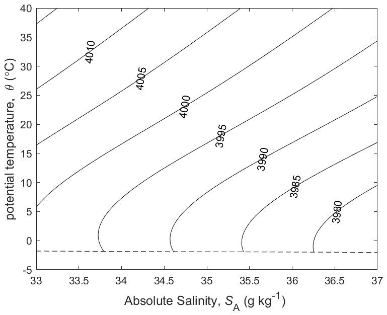
At the sea surface (P=P₀) the terms ${\stackrel{\mathrm{̃}}{h}}_{\mathit{\theta }\mathit{\theta }}$ and ${\stackrel{\mathrm{̃}}{h}}_{\mathit{\theta }{S}_{\mathrm{A}}}$ represent the variation of the specific heat capacity c_p=h_T with potential temperature and Absolute Salinity, respectively (see Fig. 1). Interestingly, when two seawater parcels at the same potential temperature but contrasting salinities are mixed, the potential temperature of the mixture is different to the initial potential temperature, this being due to the ${\stackrel{\mathrm{̃}}{h}}_{S_{\mathrm{A}}{S}_{\mathrm{A}}}$ term. The effect goes by the confusingly named “enthalpy of mixing effect”; confusing because enthalpy is conserved during this mixing process.

Figure 1 Contours of the isobaric specific heat capacity c_p (in $\mathrm{J}{\mathrm{kg}}^{-\mathrm{1}}{\mathrm{K}}^{-\mathrm{1}}$) of seawater at p = 0 dbar.

The calculation for the non-conservative production of Conservative Temperature proceeds similarly, using enthalpy in the form $\widehat{h}(S_{\mathrm{A}},\mathrm{\Theta },P)$, finding

$$\begin{array}{}\text{(27)}& \begin{array}{rl}\mathit{\delta }\mathrm{\Theta }={\displaystyle \frac{\mathrm{1}}{\mathrm{8}}}{\left({\widehat{h}}_{\mathrm{\Theta }}\right)}^{-\mathrm{1}}& \left\{{\widehat{h}}_{\mathrm{\Theta }\mathrm{\Theta }}{\left(\mathrm{\Delta }\mathrm{\Theta }\right)}^{\mathrm{2}}+\mathrm{2}{\widehat{h}}_{\mathrm{\Theta }{S}_{\mathrm{A}}}\mathrm{\Delta }\mathrm{\Theta }\mathrm{\Delta }{S}_{\mathrm{A}}\right.\\ & \left.+{\widehat{h}}_{S_{\mathrm{A}}{S}_{\mathrm{A}}}(\mathrm{\Delta }{S}_{\mathrm{A}}{)}^{\mathrm{2}}\right\}.\end{array}\end{array}$$

7.2 The causes of the non-conservation of several variables

We begin with this last expression, Eq. (27), and concentrate on the second order derivatives of $\widehat{h}(S_{\mathrm{A}},\mathrm{\Theta },P)$. The first and second Θ derivates of $\widehat{h}(S_{\mathrm{A}},\mathrm{\Theta },P)$ are expressed in terms of pressure integrals of specific volume by

$$\begin{array}{}\text{(28)}& \begin{array}{rl}{\widehat{h}}_{\mathrm{\Theta }}& =c_p^{\mathrm{0}}+{\int }_{P_{\mathrm{0}}}^P{\widehat{v}}_{\mathrm{\Theta }}\left(S_{\mathrm{A}},\mathrm{\Theta },P^{\prime }\right)\mathrm{d}{P}^{\prime },\text{ and }\\ & {\widehat{h}}_{\mathrm{\Theta }\mathrm{\Theta }}={\int }_{P_{\mathrm{0}}}^P{\widehat{v}}_{\mathrm{\Theta }\mathrm{\Theta }}\left(S_{\mathrm{A}},\mathrm{\Theta },P^{\prime }\right)\mathrm{d}{P}^{\prime },\end{array}\end{array}$$

and corresponding expressions exist for ${\widehat{h}}_{\mathrm{\Theta }{S}_{\mathrm{A}}}$ in terms of the pressure integral of ${\widehat{v}}_{\mathrm{\Theta }{S}_{\mathrm{A}}}$, and for ${\widehat{h}}_{S_{\mathrm{A}}{S}_{\mathrm{A}}}$ in terms of the pressure integral of ${\widehat{v}}_{S_{\mathrm{A}}{S}_{\mathrm{A}}}$. These expressions for the second derivatives of $\widehat{h}(S_{\mathrm{A}},\mathrm{\Theta },P)$ show that the non-conservative production of Conservative Temperature, Eq. (27), is due to the nonlinear nature of $\widehat{h}(S_{\mathrm{A}},\mathrm{\Theta },P)$ (or equivalently of $\widehat{v}(S_{\mathrm{A}},\mathrm{\Theta },P))$, as a function of S_A and Θ. Note that the non-conservative production of Θ is due to the nonlinear nature of $\widehat{h}(S_{\mathrm{A}},\mathrm{\Theta },P)$ and is independent of the nonlinear nature of $\widehat{\mathit{\eta }}(S_{\mathrm{A}},\mathrm{\Theta })$.

The non-conservation of Conservative Temperature can be further understood by considering the changes in enthalpy of two fluid parcels as they are lifted to the sea surface pressure where they are then allowed to mix, and subsequently the mixed fluid is adiabatically lowered to the original pressure. The change in enthalpy experienced during these pressure excursions is then compared with having them mix together at their original location. As the seawater parcel, parcel 1, is lifted adiabatically and without change of salinity from P_m to P₀, its enthalpy decreases by ${\int }_{P_{\mathrm{0}}}^{P_{\mathrm{m}}}\widehat{v}(S_{\mathrm{A}\mathrm{1}},{\mathrm{\Theta }}_{\mathrm{1}},P^{\prime })\mathrm{d}{P}^{\prime }$ from $\widehat{h}(S_{\mathrm{A}\mathrm{1}},{\mathrm{\Theta }}_{\mathrm{1}},P_{\mathrm{m}})$ to $\widehat{h}(S_{\mathrm{A}\mathrm{1}},{\mathrm{\Theta }}_{\mathrm{1}},P_{\mathrm{0}})=c_p^{\mathrm{0}}{\mathrm{\Theta }}_{\mathrm{1}}$ while that of parcel 2 decreases by ${\int }_{P_{\mathrm{0}}}^{P_{\mathrm{m}}}\widehat{v}(S_{\mathrm{A}\mathrm{2}},{\mathrm{\Theta }}_{\mathrm{2}},P^{\prime })\mathrm{d}{P}^{\prime }$ from $\widehat{h}(S_{\mathrm{A}\mathrm{2}},{\mathrm{\Theta }}_{\mathrm{2}},P_{\mathrm{m}})$ to $\widehat{h}(S_{\mathrm{A}\mathrm{2}},{\mathrm{\Theta }}_{\mathrm{2}},P_{\mathrm{0}})=c_p^{\mathrm{0}}{\mathrm{\Theta }}_{\mathrm{2}}$. When these parcels are mixed at P₀, Conservative Temperature is conserved so that the Conservative Temperature of the mixture is the average of Θ₁ and Θ₂ (assuming the two parcels have equal masses). When this mixed seawater parcel is now returned adiabatically to the original pressure, its specific enthalpy increases during the descent, but this increase is less than the two parcels lost during their ascent. The final enthalpy at the original pressure of the mixed fluid parcel is less than the average of the enthalpies of the two original parcels at P_m by the amount

$$\begin{array}{}\text{(29)}& \begin{array}{rl}& {\int }_{P_{\mathrm{0}}}^{P_{\mathrm{m}}}\widehat{v}\left({\displaystyle \frac{\mathrm{1}}{\mathrm{2}}}\left[S_{\mathrm{A}\mathrm{1}}+S_{\mathrm{A}\mathrm{2}}\right],{\displaystyle \frac{\mathrm{1}}{\mathrm{2}}}\left[{\mathrm{\Theta }}_{\mathrm{1}}+{\mathrm{\Theta }}_{\mathrm{2}}\right],P^{\prime }\right)\mathrm{d}{P}^{\prime }\\ & -{\displaystyle \frac{\mathrm{1}}{\mathrm{2}}}{\int }_{P_{\mathrm{0}}}^{P_{\mathrm{m}}}\widehat{v}\left(S_{\mathrm{A}\mathrm{1}},{\mathrm{\Theta }}_{\mathrm{1}},P^{\prime }\right)\mathrm{d}{P}^{\prime }\\ & -{\displaystyle \frac{\mathrm{1}}{\mathrm{2}}}{\int }_{P_{\mathrm{0}}}^{P_{\mathrm{m}}}\widehat{v}\left(S_{\mathrm{A}\mathrm{2}},{\mathrm{\Theta }}_{\mathrm{2}},P^{\prime }\right)\mathrm{d}{P}^{\prime },\end{array}\end{array}$$

which is equal to

$$\begin{array}{}\text{(30)}& \begin{array}{rl}& \widehat{h}\left({\displaystyle \frac{\mathrm{1}}{\mathrm{2}}}\left[S_{\mathrm{A}\mathrm{1}}+S_{\mathrm{A}\mathrm{2}}\right],{\displaystyle \frac{\mathrm{1}}{\mathrm{2}}}\left[{\mathrm{\Theta }}_{\mathrm{1}}+{\mathrm{\Theta }}_{\mathrm{2}}\right],P_{\mathrm{m}}\right)\\ & -{\displaystyle \frac{\mathrm{1}}{\mathrm{2}}}\widehat{h}(S_{\mathrm{A}\mathrm{1}},{\mathrm{\Theta }}_{\mathrm{1}},P_{\mathrm{m}})-{\displaystyle \frac{\mathrm{1}}{\mathrm{2}}}\widehat{h}(S_{\mathrm{A}\mathrm{2}},{\mathrm{\Theta }}_{\mathrm{2}},P_{\mathrm{m}}).\end{array}\end{array}$$

The contraction-on-mixing terms in Eqs. (27) and (28) can be recognised as a Taylor series expansion of the finite amplitude expressions in Eqs. (29) and (30). This physical argument shows that the artificial process of adiabatically moving the fluid parcels to P₀ and having the mixing process occur at this level results in a smaller Conservative Temperature of the mixed parcel than if the two fluid parcels are mixed in situ. As shown by Graham and McDougall (2013), interior mixing in the ocean always results in a positive production of Conservative Temperature.

Now considering the expression Eq. (26) for the non-conservative production of potential temperature, the first and second order θ derivatives of $\stackrel{\mathrm{̃}}{h}(S_{\mathrm{A}},\mathit{\theta },P)$ are

$$\begin{array}{}\text{(31)}& \begin{array}{rl}& {\stackrel{\mathrm{̃}}{h}}_{\mathit{\theta }}={\stackrel{\mathrm{̃}}{h}}_{\mathit{\theta }}^{\mathrm{0}}(S_{\mathrm{A}},\mathit{\theta })+{\int }_{P_{\mathrm{0}}}^P{\stackrel{\mathrm{̃}}{v}}_{\mathit{\theta }}\left(S_{\mathrm{A}},\mathit{\theta },P^{\prime }\right)\mathrm{d}{P}^{\prime },\text{ and }\\ & {\stackrel{\mathrm{̃}}{h}}_{\mathit{\theta }\mathit{\theta }}={\stackrel{\mathrm{̃}}{h}}_{\mathit{\theta }\mathit{\theta }}^{\mathrm{0}}(S_{\mathrm{A}},\mathit{\theta })+{\int }_{P_{\mathrm{0}}}^P{\stackrel{\mathrm{̃}}{v}}_{\mathit{\theta }\mathit{\theta }}\left(S_{\mathrm{A}},\mathit{\theta },P^{\prime }\right)\mathrm{d}{P}^{\prime }.\end{array}\end{array}$$

The pressure integral terms here are very similar in magnitude to those in Eq. (28), but the key difference between the expressions for ${\stackrel{\mathrm{̃}}{h}}_{\mathit{\theta }\mathit{\theta }}$ and ${\widehat{h}}_{\mathrm{\Theta }\mathrm{\Theta }}$ is the additional term ${\stackrel{\mathrm{̃}}{h}}_{\mathit{\theta }\mathit{\theta }}^{\mathrm{0}}(S_{\mathrm{A}},\mathit{\theta })$ in Eq. (31), where the superscript 0 denotes that the property is evaluated at the sea surface, specifically, at one standard atmosphere pressure P₀ = 101 325 Pa = 10.1325 dbar. The pressure integral of ${\stackrel{\mathrm{̃}}{v}}_{\mathit{\theta }\mathit{\theta }}$ in Eq. (31) is zero at the sea surface and increases in magnitude with pressure, becoming comparable with the first term, ${\stackrel{\mathrm{̃}}{h}}_{\mathit{\theta }\mathit{\theta }}^{\mathrm{0}}(S_{\mathrm{A}},\mathit{\theta })$, at ∼ 10⁸ Pa = 10 000 dbar. However, at these depths the temperature and salinity changes in the ocean are tiny compared with those in the upper ocean so the non-conservative production of potential temperature, δθ, is very small at these depths.

In order to find the root cause of the terms ${\stackrel{\mathrm{̃}}{h}}_{\mathit{\theta }\mathit{\theta }}^{\mathrm{0}}(S_{\mathrm{A}},\mathit{\theta })$, ${\stackrel{\mathrm{̃}}{h}}_{\mathit{\theta }{S}_{\mathrm{A}}}^{\mathrm{0}}(S_{\mathrm{A}},\mathit{\theta })$ and ${\stackrel{\mathrm{̃}}{h}}_{S_{\mathrm{A}}{S}_{\mathrm{A}}}^{\mathrm{0}}(S_{\mathrm{A}},\mathit{\theta })$ that cause the non-conservative production of potential temperature at P₀, the relationship $(T_{\mathrm{0}}+\mathit{\theta })=c_p^{\mathrm{0}}/{\widehat{\mathit{\eta }}}_{\mathrm{\Theta }}$ is used to write ${\stackrel{\mathrm{̃}}{h}}_{\mathit{\theta }}^{\mathrm{0}}(S_{\mathrm{A}},\mathit{\theta })=c_p^{\mathrm{0}}{\stackrel{\mathrm{̃}}{\mathrm{\Theta }}}_{\mathit{\theta }}=c_p^{\mathrm{0}}/{\widehat{\mathit{\theta }}}_{\mathrm{\Theta }}$ as $-({\widehat{\mathit{\eta }}}_{\mathrm{\Theta }}{)}^{\mathrm{2}}/{\widehat{\mathit{\eta }}}_{\mathrm{\Theta }\mathrm{\Theta }}$ and ${\stackrel{\mathrm{̃}}{h}}_{\mathit{\theta }\mathit{\theta }}^{\mathrm{0}}(S_{\mathrm{A}},\mathit{\theta })$ as $\frac{\mathrm{1}}{\mathrm{2}}\left(c_p^{\mathrm{0}}{)}^{-\mathrm{1}}\right(\left[\right({\widehat{\mathit{\eta }}}_{\mathrm{\Theta }}{)}^{\mathrm{2}}/{\widehat{\mathit{\eta }}}_{\mathrm{\Theta }\mathrm{\Theta }}{]}^{\mathrm{2}}{)}_{\mathrm{\Theta }}$. This shows that ${\stackrel{\mathrm{̃}}{h}}_{\mathit{\theta }\mathit{\theta }}^{\mathrm{0}}(S_{\mathrm{A}},\mathit{\theta })$ depends on $\widehat{\mathit{\eta }}(S_{\mathrm{A}},\mathrm{\Theta })$ and is independent of the nonlinear nature of enthalpy $\widehat{h}(S_{\mathrm{A}},\mathrm{\Theta },P)$. Making use of several results from Appendix P of IOC et al. (2010), it can be shown that the same conclusion applies to the terms ${\stackrel{\mathrm{̃}}{h}}_{\mathit{\theta }{S}_{\mathrm{A}}}^{\mathrm{0}}(S_{\mathrm{A}},\mathit{\theta })$ and ${\stackrel{\mathrm{̃}}{h}}_{S_{\mathrm{A}}{S}_{\mathrm{A}}}^{\mathrm{0}}(S_{\mathrm{A}},\mathit{\theta })$ in Eq. (26). That is, these terms are also due to the nonlinear nature of $\widehat{\mathit{\eta }}(S_{\mathrm{A}},\mathrm{\Theta })$ and are independent of the nonlinearity of $\widehat{h}(S_{\mathrm{A}},\mathrm{\Theta },P)$. We conclude that our choice of $\widehat{h}(S_{\mathrm{A}},\mathrm{\Theta },P)$ and $\widehat{\mathit{\eta }}(S_{\mathrm{A}},\mathrm{\Theta })$ to define the thermodynamic properties of seawater means that the dominant terms (the terms that apply at P₀) that cause potential temperature to not be conserved upon mixing are due to the nonlinearity in entropy $\widehat{\mathit{\eta }}(S_{\mathrm{A}},\mathrm{\Theta })$ and not due to the nonlinearity of $\widehat{h}(S_{\mathrm{A}},\mathrm{\Theta },P)$. The nonlinear nature of enthalpy plays a much smaller role and only does so deeper in the water column.

Exactly the same conclusion applies to entropy as can be seen from Eq. (25). When mixing occurs at the sea surface, Θ is a conservative variable and the second line of Eq. (25) implicates only $\widehat{\mathit{\eta }}(S_{\mathrm{A}},\mathrm{\Theta })$ in the non-conservative production of entropy. For mixing deeper in the ocean, Conservative Temperature is not totally conserved (due to the nonlinear nature of $\widehat{h}(S_{\mathrm{A}},\mathrm{\Theta },P)$, not $\widehat{\mathit{\eta }}(S_{\mathrm{A}},\mathrm{\Theta }))$ and this non-conservation adds a little to the non-conservation of entropy caused by $\widehat{\mathit{\eta }}(S_{\mathrm{A}},\mathrm{\Theta })$, because the non-conservation of Θ is sign-definite and positive (though small) and so adds to the non-conservative production of entropy. Note that the sign-definite nature of the non-conservative production-on-mixing of Θ was proven by Graham and McDougall (2013). Note that the sign-definite nature of the non-conservative production of Θ is not a consequence of the Second Law of Thermodynamics.

It is interesting that the non-conservative nature of both θ and η is mostly caused by the same nonlinear nature of entropy $\widehat{\mathit{\eta }}(S_{\mathrm{A}},\mathrm{\Theta })$, with further non-conservative production due to $\widehat{h}(S_{\mathrm{A}},\mathrm{\Theta },P)$ that applies away from the sea surface and is smaller by two or three orders of magnitude (see the next section).

When expressed in terms of constraints on the Gibbs function $g(S_{\mathrm{A}},T,P)$, it is well known from studying the instantaneous evolution equations that the Second Law of Thermodynamics requires that g_TT < 0 and $g_{S_{\mathrm{A}}{S}_{\mathrm{A}}}$ > 0. The physical interpretations of these constraints are that when a seawater parcel is heated, its temperature must increase, and that in the absence of temperature and pressure gradients, salt must molecularly diffuse down the gradient of salinity, not up this gradient. Appendix A16 of the TEOS-10 Manual (IOC et al., 2010) started from the conservative nature of enthalpy when parcels are mixed at constant pressure and proved that exactly the same pair of constraints apply in the presence of turbulent mixing processes; this result does not seem to have previously appeared in the literature.

The non-conservation of specific volume, like that of Conservative Temperature, is caused only by the nonlinear nature of enthalpy $\widehat{h}(S_{\mathrm{A}},\mathrm{\Theta },P)$ and is not affected by the non-linear nature of entropy $\widehat{\mathit{\eta }}(S_{\mathrm{A}},\mathrm{\Theta })$ This can be found by examining Eq. (24) where the terms ${\widehat{v}}_{\mathrm{\Theta }\mathrm{\Theta }}$, ${\widehat{v}}_{\mathrm{\Theta }{S}_{\mathrm{A}}}$ and ${\widehat{v}}_{S_{\mathrm{A}}{S}_{\mathrm{A}}}$ can be written as ${\widehat{h}}_{P\mathrm{\Theta }\mathrm{\Theta }}$, ${\widehat{h}}_{P\mathrm{\Theta }{S}_{\mathrm{A}}}$ and ${\widehat{h}}_{P{S}_{\mathrm{A}}{S}_{\mathrm{A}}}$, and the extra production of specific volume that occurs in the first line of Eq. (24) compared with the second line, is due to the non-conservative production of Conservative Temperature which, as we have noted below Eq. (28), is also due to the nonlinear nature of $\widehat{h}(S_{\mathrm{A}},\mathrm{\Theta },P)$ and not of $\widehat{\mathit{\eta }}(S_{\mathrm{A}},\mathrm{\Theta })$. It is also interesting to note the similar form of the dependence of the non-conservation of v and Θ on the second derivatives of specific volume. That is, the same ${\widehat{v}}_{\mathrm{\Theta }\mathrm{\Theta }}$, ${\widehat{v}}_{\mathrm{\Theta }{S}_{\mathrm{A}}}$ and ${\widehat{v}}_{S_{\mathrm{A}}{S}_{\mathrm{A}}}$ terms appear in Eqs. (24), (27) and (28), with the latter case being in the form of pressure integrals.

In conclusion, in this section we have shown that the non-conservative natures of both Conservative Temperature Θ and specific volume v are caused by the nonlinear nature of enthalpy $\widehat{h}(S_{\mathrm{A}},\mathrm{\Theta },P)$ and are independent of the non-linearity of entropy $\widehat{\mathit{\eta }}(S_{\mathrm{A}},\mathrm{\Theta })$. In contrast, the non-conservative natures of both potential temperature and entropy are predominantly due to the nonlinear nature of entropy $\widehat{\mathit{\eta }}(S_{\mathrm{A}},\mathrm{\Theta })$, with only a very minor contribution, at large pressures, from the nonlinear nature of enthalpy $\widehat{h}(S_{\mathrm{A}},\mathrm{\Theta },P)$.

Before closing this section, we discuss the non-conservative production of internal energy u and of total energy $E\equiv u+K+\mathrm{\Phi }$. Figure 2 shows a water column on the left before a mixing event occurs in the shaded fluid which contains variations in Conservative Temperature and Absolute Salinity. The right-hand water column is the situation after the mixing event. The mixing process takes place at pressure P_m. Because of the non-conservative behaviour of specific volume, the volume of the final mixed fluid is less than that of the initial unmixed fluid and all the water parcels in the water column above the mixing event retain their pressure, internal energy, enthalpy, but suffer a loss of height and of gravitational potential energy. All these fluid parcels experience a change in their total energy E even though they have not experienced a mixing event (McDougall et al., 2003). This occurs because total energy $E\equiv u+K+\mathrm{\Phi }$ is not a thermodynamic quantity, that is, it depends not only on $(S_{\mathrm{A}},\mathrm{\Theta },P)$ but also on the extra quantities, kinetic energy and gravitational potential energy, which are not governed by thermodynamics alone.

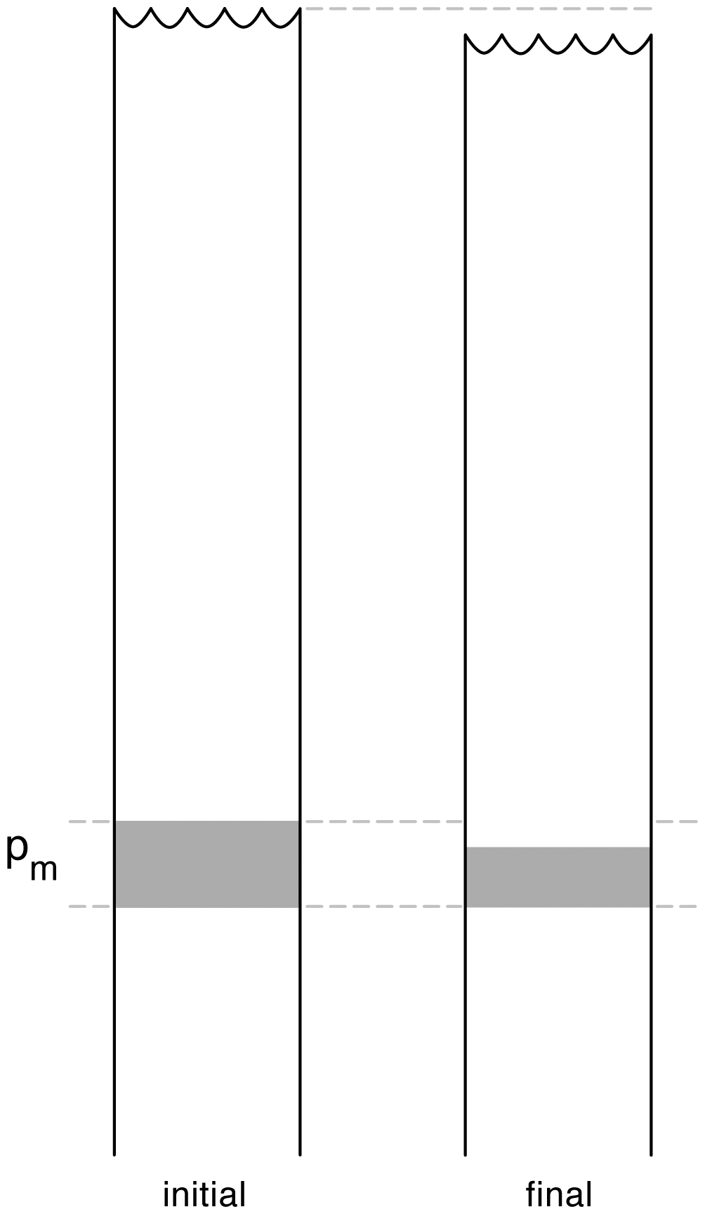
Figure 2 Diagram illustrating the non-conservation of internal energy and Total Energy (from McDougall et al., 2003). At the location of the mixing, specific volume decreases while both internal energy u and total energy E increase. During the mixing event the entire water column above the mixing height slumps downwards. Seawater parcels above the mixing event all have unchanged values of internal energy, enthalpy and potential enthalpy, but they have decreased values of total energy (due to the reduced gravitational potential energy caused by the slumping).

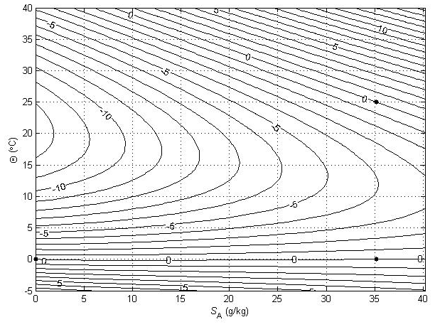
Figure 3 Contours (in °C) of a variable that is used to illustrate the non-conservative production of specific volume at p = 0 dbar (where Θ is a conservative variable). The variable is forced to be zero at the three points shown with black dots.

Concentrating now on the fluid that undergoes the mixing in Fig. 2, if we ignore any changes in kinetic energy, the non-conservative production of total energy δE is the same as that of internal energy, δu. Since both the pressure and the total amount of enthalpy of the fluid being mixed are unchanged during the mixing process (δh=0 and P=P_m), the definition of enthalpy as $h=u+Pv$ shows that the non-conservative production of internal energy is δu = −P_mδv. When examining Eqs. (24), (27) and (28) we find an approximate relationship between the non-conservative production of v and of Θ, namely $c_p^{\mathrm{0}}\mathit{\delta }\mathrm{\Theta }\cong -(P_{\mathrm{m}}-P_{\mathrm{0}})\mathit{\delta }v\cong -P_{\mathrm{m}}\mathit{\delta }v$ = δu = δE. This approximation relies on the second derivative terms such as ${\widehat{v}}_{\mathrm{\Theta }\mathrm{\Theta }}$ in Eq. (28) not being strong functions of pressure.

Another interesting example occurs when considering the input of a certain amount of heat into a kilogram of seawater, in the first case at P₀, and in the second case where this same amount of heat is used to warm a kilogram of seawater at some greater pressure. The increase in the enthalpies of the two seawater parcels is the same in both cases, but the increases in their Conservative Temperatures are in the ratio $(T_{\mathrm{0}}+t)/(T_{\mathrm{0}}+\mathit{\theta })$ = ${\widehat{h}}_{\mathrm{\Theta }}/c_p^{\mathrm{0}}$ (see Eq. 17) where these quantities are evaluated at the deeper parcel's pressure. The increases in the internal energies of the two seawater parcels are also unequal, with the difference being the increase in the gravitational potential energy of the whole water column (McDougall et al. 2003) in the second case. These comments apply even when the equation of state is linear in the sense that ${\widehat{v}}_{\mathrm{\Theta }}$ and ${\widehat{v}}_{S_{\mathrm{A}}}$ are constants, independent of salinity, temperature and pressure. In that case ${\widehat{h}}_{\mathrm{\Theta }}$ = $c_p^{\mathrm{0}}+{\widehat{v}}_{\mathrm{\Theta }}(P-P_{\mathrm{0}})$ while the non-conservative productions of specific volume, Conservative Temperature and internal energy are all zero. This discussion makes clear that a boundary flux of heat (for example, the geothermal heat flux) should be converted into a flux of Conservative Temperature using the specific heat capacity ${\widehat{h}}_{\mathrm{\Theta }}$; a fact that is particularly clear as it applies even for a linear equation of state for which Conservative Temperature is a 100 % conservative variable.

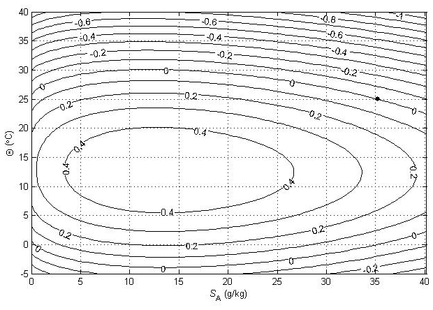
Figure 4 Contours (in °C) of a variable that is used to illustrate the non-conservative production of specific entropy at p = 0 dbar (where Θ is a conservative variable).

7.3 Comparing the non-conservation of several variables

The relationships (24)–(27) are illustrated in Figs. 3–6; these figures are explained in more detail in Sects. A16–A19 of the TEOS-10 Manual (IOC et al., 2010). The variable that is contoured in Fig. 3 was formed by first subtracting from specific volume the linear function of Absolute Salinity that made the result zero at the two (S_A,Θ) locations (0 g kg⁻¹, 0 °C) and (35.16504 g kg⁻¹, 0 °C), second by scaling the result to be equal to 25 °C at (35.16504 g kg⁻¹, 25 °C) and third, subtracting Conservative Temperature Θ. If specific volume at 0 dbar were a linear function of Absolute Salinity and Conservative Temperature, Fig. 3 would be populated with zeros. Instead, what is contoured in this figure enables us to evaluate the non-linearity of specific volume on the (S_A,Θ) diagram, expressed in °C. Specifically, the contoured variable indicates what warming or cooling would be required to account for the difference between the actual specific volume and a linear equation of state version of specific volume, using the thermal expansion coefficient applicable at S_A = 35.16504 g kg⁻¹, Θ≈ 12.5 °C and p = 0 dbar. The main use of these Figs. 3–6 is in estimating the relative magnitudes of the non-conservative production/destruction of various thermodynamic variables. As an example, consider the mixing of equal masses of the seawater parcels at (0 g kg⁻¹, 0 °C) and (35.16504 g kg⁻¹, 25 °C). From Fig. 3 we see that the mixture, at the mid-point Absolute Salinity and Conservative Temperature, would require warming by approximately 7.5 °C in order for its specific volume to be the average of the specific volumes of the two original seawater parcels.

Figure 4 is the corresponding plot for entropy, with the variable that is contoured being specific entropy multiplied by a dimensional constant so that the result is 25 °C at (35.16504 g kg⁻¹, 25 °C) and then Conservative Temperature Θ is subtracted. When the same two seawater parcels, (0 g kg⁻¹, 0 °C) and (35.16504 g kg⁻¹, 25 °C), are mixed in equal proportions, Fig. 4 shows that the entropy produced is the same as would be produced by approximately 0.45 °C of warming.

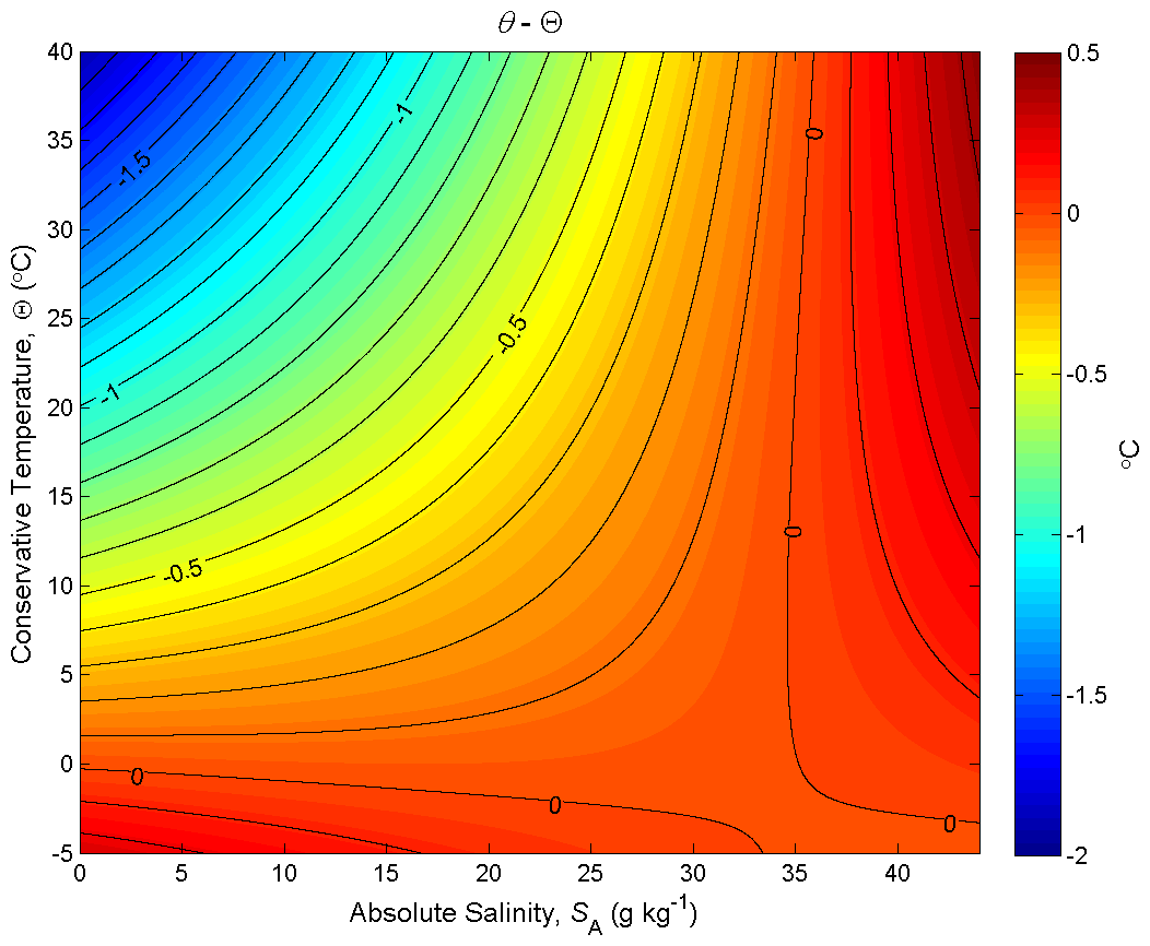
Figure 5 Contours of the difference between potential temperature and Conservative Temperature, θ−Θ (in °C), at p = 0 dbar (where Θ is a conservative variable). This plot illustrates the non-conservative behaviour of potential temperature.

Figure 5 is the corresponding plot for potential temperature, with the contours being the difference between potential temperature and Conservative Temperature, θ−Θ, at p = 0 dbar. When the same two seawater parcels, (0 g kg⁻¹, 0 °C) and (35.16504 g kg⁻¹, 25 °C), are mixed in equal proportions, Fig. 5 shows that the potential temperature of the mixture is less than its Conservative Temperature by approximately 0.35 °C. In this case the non-conservative behaviour of potential temperature has acted to destroy (rather than produce) potential temperature. If potential temperature were carried as the model's temperature variable in an ocean model, the potential temperature would be conserved during this mixing process and so the potential temperature would be overestimated by 0.35 °C. In this way the damage done by assuming potential temperature is conservative is as much as 78 % of the damage that would be done if entropy were taken to be a conservative variable (78 % being $\mathrm{0.35}/\mathrm{0.45}$ of 100 %, with the 0.45 °C figure coming from the previous paragraph, representing the actual production of entropy). This 0.78 ratio of the non-conservations of potential temperature and entropy occurs for any mixing process occurring along the line joining (0 g kg⁻¹, 0 °C) and (35.16504 g kg⁻¹, 25 °C). The curvature of the isolines on Fig. 5 changes sign at the higher salinities and in this region of (S_A,Θ) space the non-conservative production of potential temperature is positive.

While it is possible to consider the non-conservative production when pairs of parcels mix on Fig. 5, how can we obtain a realistic measure of the total effects of such non-conservation as reflected in the present ocean state. That is, we cannot sum up all the unknowable number of individual non-conservation events that have occurred in the past 1000 years in all of the ocean. It turns out that the contoured variable of Fig. 5, θ−Θ, is a good estimate of the error that is made by interpreting an ocean model's temperature variable as potential temperature. This is literally the case for an ocean model that is driven by imposed air–sea heat fluxes, and the same error measure approximately applies when the air–sea boundary condition is a combination of restoring and flux conditions. This error is easily avoided by simply interpreting the ocean model's temperature variable as Conservative Temperature (see McDougall et al. (2021a) and the following section of this review).

We come now to the non-conservative production of Conservative Temperature illustrated in Fig. 6. Since Conservative Temperature is a conservative variable for mixing at the sea surface, we illustrate its non-conservation at a pressure of 600 dbar where its non-conservation is maximised (McDougall, 2003). Enthalpy evaluated at 600 dbar is a conservative quantity for mixing processes at this pressure and this is used as the vertical axis of Fig. 6. When again considering the mixing of equal masses of the seawater parcels at (0 g kg⁻¹, 0 °C) and (35.16504 g kg⁻¹, 25 °C) (two of the bold black dots on Fig. 6) we see that the non-conservative production of Conservative Temperature amounts to 0.002 °C (2 mK).

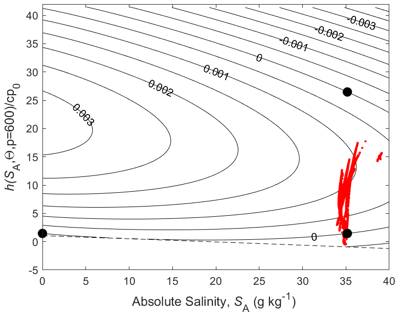
Figure 6 Contours (in °C) of a variable that is used to illustrate the non-conservative production of Conservative Temperature at p = 600 dbar where $\widehat{h}(S_{\mathrm{A}},\mathrm{\Theta },p=\mathrm{600}\mathrm{dbar})$ is a conservative variable. The variable is forced to be zero at the three points shown with black dots.

On the basis of the above examination of mixing between the seawater parcels (0 g kg⁻¹, 0 °C) and (35.16504 g kg⁻¹, 25 °C), the relative importance of the non-conservation of the three variables η, θ and Θ in the ocean would seem to be in the ratio $\mathrm{450}:\mathrm{350}:\mathrm{2}$, or $\mathrm{250}:\mathrm{175}:\mathrm{1}$. On the other hand, simply looking at the maximum contoured values in Figs. 4, 5 and 6 one might guess that the relevant ratio of the relative extent of the non-conservation of these variables is $\mathrm{0.5}:\mathrm{1.8}:\mathrm{0.003}$, or $\mathrm{167}:\mathrm{600}:\mathrm{1}$. However, neither of these estimates considers the ranges of salinity and temperature over which the interior mixing processes occur in the ocean. To do this Graham and McDougall (2013) evaluated these non-conservative production terms in an ocean model. The first step in doing this was to develop the evolution equations for these variables in a turbulent ocean, and this was based on the knowledge that enthalpy is conserved when mixing proceeds between fluid parcel at a given pressure, as we have discussed in Sect. 3.2 above.

Graham and McDougall (2013) began with our Eq. (12) above which applies instantaneously prior to averaging over unresolved turbulent motions. This equation was then averaged over turbulent motions including lateral mesoscale motions, which are then parameterized with an epineutral (that is, along the neutral tangent plane) scalar diffusivity K, and small-scale isotropic turbulence which is parameterised with an isotropic small-scale turbulent diffusivity D. The resulting evolution equation for potential enthalpy referenced to the pressure of the mixing processes, in Boussinesq form, is

$$\begin{array}{}\text{(32)}& \begin{array}{rl}& \mathrm{d}{h}^{\mathrm{m}}/\mathrm{d}t={\mathit{\gamma }}_z{\mathrm{\nabla }}_n\cdot \left({\mathit{\gamma }}_z^{-\mathrm{1}}K{\mathrm{\nabla }}_n{h}^{\mathrm{m}}\right)+{\left(D{h}_z^{\mathrm{m}}\right)}_z+\mathit{\epsilon }\\ & \text{ at }P=P_{\mathrm{m}},\end{array}\end{array}$$

where the total derivative, $\mathrm{d}{h}^{\mathrm{m}}/\mathrm{d}t$, is with respect to the Temporal-Residual Mean velocity of McDougall and McIntosh (2001), and h^m here is the thickness-weighted value, having been averaged between closely spaced neutral density (γ) surfaces; also, in the following equation Θ and S_A are also the thickness-weighted values. Graham and McDougall then exploited the fact that at the pressure P_m of a particular mixing event, the potential enthalpy $h^{\mathrm{m}}=\widehat{h}(S_{\mathrm{A}},\mathrm{\Theta },P_{\mathrm{m}})$ is a function only of Absolute Salinity and Conservative Temperature, arriving at the evolution equation for Θ in a turbulent ocean,

$$\begin{array}{}\text{(33)}& \begin{array}{rl}\mathrm{d}\mathrm{\Theta }/\mathrm{d}t=& {\mathit{\gamma }}_z{\mathrm{\nabla }}_n\cdot \left({\mathit{\gamma }}_z^{-\mathrm{1}}K{\mathrm{\nabla }}_n\mathrm{\Theta }\right)+(D{\mathrm{\Theta }}_z{)}_z+\mathit{\epsilon }/{\widehat{h}}_{\mathrm{\Theta }}\\ & +K{\left({\widehat{h}}_{\mathrm{\Theta }}\right)}^{-\mathrm{1}}\left({\widehat{h}}_{\mathrm{\Theta }\mathrm{\Theta }}{\mathrm{\nabla }}_n\mathrm{\Theta }\cdot {\mathrm{\nabla }}_n\mathrm{\Theta }\right.\\ & \left.+\mathrm{2}{\widehat{h}}_{\mathrm{\Theta }{S}_{\mathrm{A}}}{\mathrm{\nabla }}_n\mathrm{\Theta }\cdot {\mathrm{\nabla }}_n{S}_{\mathrm{A}}+{\widehat{h}}_{S_{\mathrm{A}}{S}_{\mathrm{A}}}{\mathrm{\nabla }}_n{S}_{\mathrm{A}}\cdot {\mathrm{\nabla }}_n{S}_{\mathrm{A}}\right)\\ & +D({\widehat{h}}_{\mathrm{\Theta }}{)}^{-\mathrm{1}}\left({\widehat{h}}_{\mathrm{\Theta }\mathrm{\Theta }}{\mathrm{\Theta }}_z^{\mathrm{2}}+\mathrm{2}{\widehat{h}}_{\mathrm{\Theta }{S}_{\mathrm{A}}}{\mathrm{\Theta }}_z{S}_{{\mathrm{A}}_z}\right.\\ & \left.+{\widehat{h}}_{S_{\mathrm{A}}{S}_{\mathrm{A}}}{S}_{{\mathrm{A}}_z}{S}_{{\mathrm{A}}_z}\right).\end{array}\end{array}$$

The same approach was used to develop the evolution equations for potential temperature and for specific entropy. In each case the non-conservative production terms in the evolution equation have terms that are immediately recognisable from the corresponding terms in the two-parcel mixing expressions (25)–(27).

Graham and McDougall (2013) vertically integrated the non-conservative production terms in these evolution equations for Θ, θ and η finding values of the air–sea heat flux, as a function of longitude and latitude, that equal the depth-integrated non-conservative source terms. Figure 7 shows the results as a histogram of these equivalent air–sea heat fluxes. The relative magnitudes of the non-conservation of these variables can be gauged from the values greater than which only 5 % of the values occur; these values are 1200 mW m⁻² (1.2 W m⁻²) for specific entropy η, 120 mW m⁻² for potential temperature θ, and 1 mW m⁻² for Conservative Temperature Θ. That is, the relative amounts by which η, θ and Θ are not conservative in the ocean are $\mathrm{1200}:\mathrm{120}:\mathrm{1}$ rather than the previously mentioned values of these ratios. In addition, Graham and McDougall (2013) found that the mean effective air–sea flux due to the non-conservation of Conservative Temperature is approximately 0.3 mW m⁻², and that if the air–sea flux arrives into the ocean deeper by 25 m than the depth at which most of this heat flux leaves the ocean, this leads to a mis-estimation of the net air–sea heat flux of 0.6 mW m⁻² (McDougall et al., 2021a). These values can be compared with the mean value of the depth-integrated dissipation of turbulent kinetic energy which is approximately 10 mW m⁻², demonstrating that the non-conservation of Conservative Temperature due to mixing processes is less important by a factor of at least ten than the neglect of the dissipation of turbulent kinetic energy as a source of ocean warming.

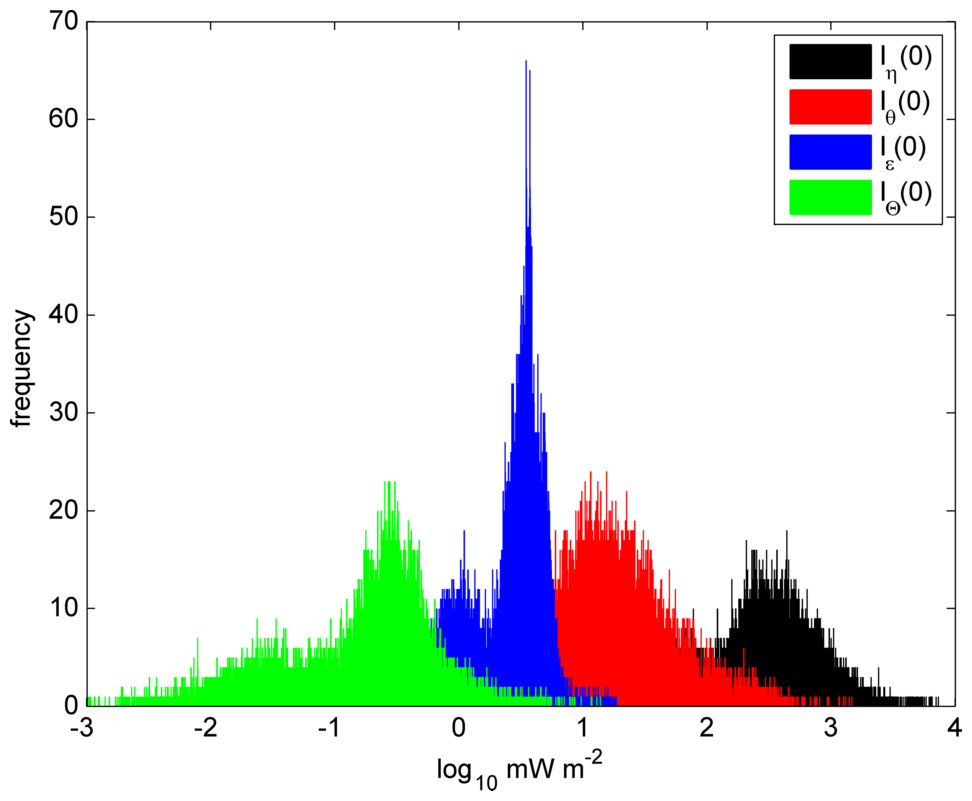
Figure 7 Histogram of the magnitude of the depth-integrated non-conservative source terms of various variables throughout the world's oceans (from Graham and McDougall, 2013). 5 % of the data points in these histograms exceed 1 mW m⁻² for Conservative Temperature Θ, 10 mW m⁻² for the dissipation of turbulent kinetic energy ε, 120 mW m⁻² for potential temperature θ, and 1200 mW m⁻² for specific entropy η.

The five steps that have led to these estimates of the non-conservation of various thermodynamic variables are

• 1.

  realizing that enthalpy is a conservative quantity when mixing occurs at fixed pressure,

• 2.

  noting that potential enthalpy $h^{\mathrm{m}}=\widehat{h}(S_{\mathrm{A}},\mathrm{\Theta },P_{\mathrm{m}})$ referenced to the pressure of a mixing event, P_m, is also conserved during the mixing event, and has the advantage over enthalpy itself in that h^m is unchanged during the variations in pressure that predate the mixing event,

• 3.

  deriving the evolution equation for $h^{\mathrm{m}}=\widehat{h}(S_{\mathrm{A}},\mathrm{\Theta },P_{\mathrm{m}})$ in a turbulent ocean by carefully averaging the First Law of Thermodynamics,

• 4.

  using this equation to find evolution equations for Conservative Temperature, potential temperature and entropy, which include the relevant non-conservative production terms, and

• 5.

  evaluating the magnitudes of the non-conservative terms in these evolution equations.

Having concentrated above on the typical, or root-mean-square values of the non-conservation of various oceanographic variables, we also mention that an extreme value of θ−Θ of − 1.5 °C occurs when warm fresh river water (e.g. the Amazon) flows into the ocean. That is, the enthalpy per unit mass of this river water is proportional to its transport of Conservative Temperature which is 1.5 °C greater than potential temperature for this warm fresh water.

In this section we have discussed how to quantify the non-conservative production of various thermodynamic variables when two seawater parcels are mixed. Traditionally a given temperature difference (perhaps 1 °C) and salinity difference were considered, and on finding that the non-conservative production of say potential temperature under turbulent mixing is small in some sense, concluding that this measure of production is typical of the damage done by taking potential temperature to be a conservative variable. But this reasoning ignores the question of how many such mixing events occur in the lifetime of a given water mass in the ocean (McDougall, 2003). Each such mixing event contributes to the non-conservative production in an additive manner. One way of quantifying the effects of all these past mixing processes is that summarised in Fig. 7, being the depth-integrated non-conservation, expressed as a surface heat flux (Graham and McDougall, 2013). Figure 7 well describes the relative magnitudes of the non-conservation of several potential heat-like variables, but we also need to know the absolute magnitude of the damage done to the modelled potential temperature when its non-conservation is ignored. This can be deduced from the following thought experiment. Imagine conducting a long ocean model run that is forced by a given surface heat flux field as a function of longitude and latitude. The temperature variable in such a run is clearly Conservative Temperature and if it is interpreted as being potential temperature, the error in such an interpretation is as displayed in the θ−Θ plot of Fig. 5. With different choices of boundary condition, the error involved with ignoring the non-conservative production of potential temperature will be similar to that displayed in Fig. 5. This thought process circumvents the issue relating to the unknowable number of mixing events in the lifetime of a water mass, and, based on the depth-integrated result of Fig. 7 we deduce that the error in ignoring the non-conservative production term of Conservative Temperature is approximately 1 % of that of potential temperature.

8 Absolute Salinity, Preformed Salinity, Reference Salinity and Practical Salinity

The derived thermodynamic property of seawater of most importance in physical oceanography is the specific volume, or density. Between 1980 and 2010 specific volume was evaluated using the EOS-80 equation which was a function of Practical Salinity, in-situ temperature and pressure (Fofonoff, 1985). Measurements of temperature and pressure at sea can be made relatively accurately compared to those of Practical Salinity, and since 1948 the International Association for the Physical Sciences of the Oceans (IAPSO) has encouraged the use of ampules of Standard Seawater of known conductivity ratio and known Practical Salinity to assist in measuring Practical Salinity at sea as accurately as possible (Smythe-Wright et al., 2019). This service is now performed by a private company, Ocean Scientific International Limited (Jenkins and Williams, 2025) which supplies bottles of IAPSO Standard Seawater. With great care it is possible to measure Practical Salinity with an accuracy of 0.003 (two standard deviations), and continuing research is encouraged to ensure this accuracy is maintained into the future, and if possible, improved (Uchida et al., 2025). Two possible routes for improvements are via the use of vibrating beam densimeters that measure density in an SI-traceable manner (Wright et al., 2011), and refractive index sensors (Uchida et al., 2019; Li et al., 2023; Yang et al., 2024; Bai et al., 2025; Zhao et al., 2025), but these possible future avenues for improvement will not be further mentioned in this article.

Practical Salinity is based on a measurement of the electrical conductivity ratio of seawater, corrected for the temperature and pressure of the seawater sample. TEOS-10 (the International Thermodynamic Equation of Seawater – 2010) recognises that the relative concentrations of the constituents of sea salt in seawater vary throughout the ocean, and these variations influence the electrical conductivity differently to how these same variations affect specific volume. Pawlowicz (2010), Wright et al. (2011) and IOC et al. (2010) discuss the several contenders for the title of the “absolute salinity” of seawater, namely “Solution Salinity”, “Added-Mass Salinity”, and “Density Salinity”. The paper of Wright et al. (2011) presents a clear and readable account of this difficult subject. Under TEOS-10 the capitalized words Absolute Salinity and the symbol S_A are reserved for “Density Salinity” such as can be deduced using laboratory measurements with a vibrating beam densimeter. That is, Absolute Salinity is defined to be that salinity that when used as the salinity argument of the TEOS-10 expression for specific volume, gives the actual specific volume of the seawater sample. Absolute Salinity is expressed on the Reference-Composition Salinity Scale of Millero et al. (2008) and is designed to be very close to the mass fraction of sea salt (non-water) in a seawater sample of Reference Composition.

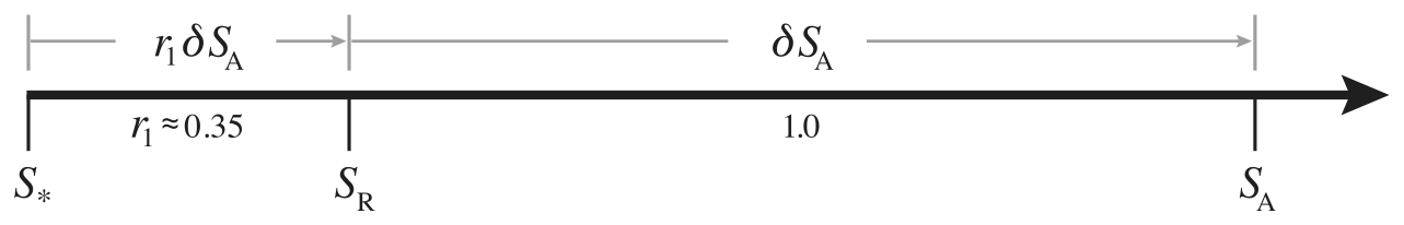
Figure 8 Number line of Salinity, illustrating the relative differences between Preformed Salinity S_∗, Reference Salinity S_R, and Absolute Salinity S_A for a seawater sample whose composition is different to that of Standard Seawater.

TEOS-10 concentrates on four different salinity variables, namely Practical Salinity S_P, Reference Salinity S_R, Absolute Salinity S_A, and Preformed Salinity S_∗. Underlying these salinity variables is the paper of Millero et al. (2008) which defined the composition of Reference-Composition Seawater as a table of exact mole fractions of the main chemical constituents of seawater. This table defines the best estimate of the composition of Standard Seawater, which is seawater from the surface waters of a certain region of the North Atlantic. For seawater of Reference Composition, its Absolute Salinity is related to Practical Salinity by

$$\begin{array}{}\text{(34)}& S_{\mathrm{R}}=u_{\text{PS}}{S}_{\mathrm{P}},\text{ where }{u}_{\text{PS}}\equiv (\mathrm{35.16504}/\mathrm{35})\mathrm{g}{\mathrm{kg}}^{-\mathrm{1}},\end{array}$$

and S_R is called the Reference Salinity. In this way, a seawater sample of Reference Composition whose Practical Salinity S_P is 35 has a Reference Salinity S_R of 35.16504 g kg⁻¹. Millero et al. (2008) estimate that the absolute uncertainty in this value is ± 0.007 g kg⁻¹. The difference between the numerical values of Reference and Practical Salinities can be traced back to the original practice of determining salinity by evaporation of water from seawater and weighing the remaining solid material. This process also evaporated some volatile components and most of the 0.16504 g kg⁻¹ salinity difference is due to this effect.

If the composition of a seawater sample is different to that of Reference-Composition Seawater, then its Reference Salinity can still be calculated using Eq. (34) (this is the Absolute Salinity of the sample under the assumption that the sample is of Reference Composition) and the sample's Absolute Salinity is calculated as

$$\begin{array}{}\text{(35)}& S_{\mathrm{A}}=S_{\mathrm{R}}+\mathit{\delta }{S}_{\mathrm{A}},\end{array}$$

where δS_A is called the Absolute Salinity Anomaly and is usually evaluated from the computer software of the Gibbs SeaWater Oceanographic Toolbox (McDougall and Barker, 2011). This approach for estimating the Absolute Salinity Anomaly is actually based on laboratory measurements of the density of seawater samples collected from around the world's oceans as described in McDougall et al. (2012). However, if open ocean measurements are available of the Total Alkalinity, Dissolved Inorganic Carbon, and the nitrate and silicate concentrations, then an alternative formula is available to calculate Absolute Salinity according to the expression,

$$\begin{array}{}\text{(36)}& \begin{array}{rl}(S_{\mathrm{A}}-S_{\mathrm{R}})/\left(\mathrm{g}{\mathrm{kg}}^{-\mathrm{1}}\right)=& (\mathrm{55.6}\mathrm{\Delta }\mathrm{TA}+\mathrm{4.7}\mathrm{\Delta }\mathrm{DIC}\\ & +\mathrm{38.9}{\mathrm{NO}}_{\mathrm{3}}^{-}+\mathrm{50.7}\mathrm{Si}(\mathrm{OH}{)}_{\mathrm{4}})/\\ & \left(\mathrm{mol}{\mathrm{kg}}^{-\mathrm{1}}\right).\end{array}\end{array}$$

This approach was developed by Pawlowicz et al. (2011) using a chemical model of the electrical conductivity and density of seawater. This equation is written in terms of the values of the nitrate and silicate concentrations in the seawater sample (measured in mol kg⁻¹), the differences ΔTA and ΔDIC, between the Total Alkalinity (TA) and Dissolved Inorganic Carbon (DIC) of the sample and the corresponding values of our best estimates of TA and DIC in Standard Seawater. For Standard Seawater our best estimates of TA and DIC are 0.0023 ($S_{\mathrm{P}}/\mathrm{35}$) mol kg⁻¹ and 0.00208 ($S_{\mathrm{P}}/\mathrm{35}$) mol kg⁻¹, respectively (see the discussion in Wright et al., 2011).

Preformed Salinity S_∗ is designed to be a conservative salinity variable which is unaffected by biogeochemical activity in the ocean; it is defined as Absolute Salinity minus the contributions of biogeochemical processes to Absolute Salinity. Based on the work of Pawlowicz et al. (2011) the difference between Absolute Salinity and Preformed Salinity is approximately proportional to the difference between Absolute Salinity and Reference Salinity, with the proportionality constant being 1.35. That is, $(S_{\mathrm{A}}-S_{\ast })\approx \mathrm{1.35}(S_{\mathrm{A}}-S_{\mathrm{R}})$, and this is illustrated in Fig. 8. As we discuss in Sect. 9 below, the salinity in present ocean models is best interpreted as Preformed Salinity, and as biogeochemical ocean models improve it is hoped that the Absolute Salinity during the running of an ocean model will be calculated using the model's ΔTA, ΔDIC, nitrate and silicate values according to the analogous equation to Eq. (36) above, namely

$$\begin{array}{}\text{(37)}& \begin{array}{rl}(S_{\mathrm{A}}-S_{\ast })/\left(\mathrm{g}{\mathrm{kg}}^{-\mathrm{1}}\right)=& (\mathrm{73.7}\mathrm{\Delta }\mathrm{TA}+\mathrm{11.8}\mathrm{\Delta }\mathrm{DIC}\\ & +\mathrm{81.9}{\mathrm{NO}}_{\mathrm{3}}^{-}+\mathrm{50.6}\mathrm{Si}(\mathrm{OH}{)}_{\mathrm{4}})/\\ & \left(\mathrm{mol}{\mathrm{kg}}^{-\mathrm{1}}\right).\end{array}\end{array}$$

which is Eq. (A.4.14) of IOC et al. (2010) and Eq. (10) of Wright et al. (2011). Ocean models that do not carry biogeochemistry and so are unable to evaluate Eq. (37) should use the method described in IOC et al. (2010), Wright et al. (2011), McDougall and Barker (2011) and McDougall et al. (2013), which essentially involves a relaxation to present day observations of silicic acid.

This section has just scratched the surface of this subject of salinity. The interested reader will find more details on the various salinity variables in previous review articles on the thermodynamics of seawater (McDougall et al. 2013, Pawlowicz et al. 2016 and Feistel, 2018), and in the rather comprehensive Wright et al. (2011) paper.

9 The temperature and salinity variables of ocean models

This section will show that because ocean models to date have not included non-conservative source terms in their evolution equations for either temperature or salinity, the model's temperature and salinity must be interpreted as Conservative Temperature Θ and Preformed Salinity S_∗. It is observation-derived fields of Θ and S_∗ that should be used to both initialize these ocean models and to compare with model output. During the running of an ocean model, if the air–sea heat flux is parameterized using a bulk formula based on potential temperature θ at the sea surface (SST), then potential temperature needs to be calculated at run time using the relationship $(T_{\mathrm{0}}+\mathit{\theta })=c_p^{\mathrm{0}}/{\widehat{\mathit{\eta }}}_{\mathrm{\Theta }}$ using entropy in the functional form $\widehat{\mathit{\eta }}(S_{\mathrm{A}},\mathrm{\Theta })$ (McDougall et al., 2023).

The following Sect. 9.1 discusses the correct interpretation of model salinity and shows that the neglect to date of estimating Absolute Salinity in ocean models has led all these models to misestimate the meridional overturning transport of key water masses by ∼ 13.5 %. Section 9.2 goes on to show that the temperature variable in ocean models should be interpreted as being Conservative Temperature, and if one insists that the model temperature is potential temperature, then up to 0.3 W m⁻² of the air–sea heat flux is lost in some regions; that is, up to 0.3 W m⁻² leaves the atmosphere but does not arrive in the ocean. Such non-conservative spontaneous heat loss should no longer be countenanced when examining the output of climate models.

9.1 The salinity of ocean models is Preformed Salinity S_∗

The influence of biogeochemistry on salinity, specific volume and the thermal wind equation has been ignored in ocean modelling to date. Biogeochemistry causes spatial variations in the relative concentrations of the constituents of sea salt (particularly variations in silicic acid concentration), and these spatial differences have been ignored and so have not been allowed to affect the model's salinity and specific volume. If an ocean model carried several biogeochemical variables, then the Absolute Salinity S_A could be calculated as an addition to the model's Preformed Salinity S_∗ using Eq. (37). In this approach, the ocean model continues to carry Preformed Salinity S_∗ as its salinity prognostic variable and evaluates Absolute Salinity S_A using Eq. (37) just before every call to the equation of state. This method has not yet been implemented by an ocean model. An alternative method of allowing for the variations of seawater composition by relaxing towards existing observations of these quantities has been outlined in IOC et al. (2010), Wright et al. (2011), McDougall and Barker (2011) and McDougall et al. (2013), but this method has also not been implemented to date.

Ocean models initialize their salinity as Reference Salinity (or, in the EOS-80 case, as Practical Salinity). At the sea surface the concentration of nutrients and silicic acid is very small so that Reference Salinity at the sea surface is virtually the same as Preformed Salinity (and Absolute Salinity). Since ocean models are initialized (and usually restored) to surface values of Preformed Salinity, and since both the models' salinity and Preformed Salinity are conservative, then the output salinity of models has only one interpretation, namely Preformed Salinity (or $S_{\ast }/u_{\text{PS}}$ in the case of an EOS-80 based ocean model, see Eq. 34).

How large might be the influence of neglecting ($S_{\mathrm{A}}-S_{\ast }$) in ocean models? From Sects. A5 and A20 of the TEOS-10 Manual (IOC et al., 2010) we see that of the ocean that is deeper than 1000 dbar in the World Ocean, 58 % of the locations would misestimate the thermal wind balance by more than 2 % due to ignoring the difference (S_A−S_R) between Absolute and Reference Salinities. The corresponding misestimation in an ocean model context, namely the effect on the thermal wind balance arising from ($S_{\mathrm{A}}-S_{\ast }$) is 2.7 %, being larger than 2 % by a factor of 1.35 (Fig. 8). This is not a good situation for our field of physical oceanography, with approximately half of the locations deeper than 1000 m in ocean models having thermal wind errors of greater than 3 %. This should be rectified as soon as possible.

McCarthy et al. (2015) studied the influence of using Absolute Salinity versus Reference Salinity in calculating the overturning circulation in the North Atlantic. They found that the overturning streamfunction changed by 0.7 Sv at a depth of 2700 m, relative to a mean value at this depth of about 7 Sv, i.e., a 10 % effect. Since the salinity variable in ocean models is actually Preformed Salinity, the neglect of the distinction between Preformed and Absolute Salinities in ocean models means that they currently misestimate the overturning streamfunction at this depth by 1.35 (see Fig. 8) times 0.7 Sv, namely ∼ 1 Sv, which is 13.5 % of the overturning streamfunction. It surely is high time to include a scheme in ocean models to account for the difference between Absolute Salinity and the model's Preformed Salinity in order to avoid these transport errors of order 13.5 %.

As a final remark on salinity in ocean models, we emphasise that even though ocean models that use the EOS-80 equation of state usually describe their salinity variable as being Practical Salinity, this is not the case. These models do not include the non-conservative term that appears in the evolution equation for Practical Salinity, and so the correct interpretation of the salinity variable in these models is $S_{\ast }/u_{\text{PS}}$. These issues are discussed in greater detail in McDougall et al. (2021a). We conclude that because ocean models, of both the TEOS-10 and EOS-80 variety, treat their salinity variable as being conservative, the salinity variable is neither Absolute Salinity nor Reference Salinity (nor Practical Salinity in the case of EOS-80 models) but rather is Preformed Salinity S_∗ (or $S_{\ast }/u_{\text{PS}}$ in the case of EOS-80 models). The neglect of any attempt in ocean models to enable the evaluation of specific volume using Absolute Salinity means that overturning transports are currently in error by an estimated 13.5 %.

9.2 The temperature of ocean models is Conservative Temperature Θ

The air–sea heat flux in ocean models is related to the sea surface flux of the model's temperature variable using a fixed value of the specific heat $c_p^{\mathrm{0}}$. This is clearly appropriate when the model temperature is interpreted as being Conservative Temperature as it is in TEOS-10 based ocean models, but what are the implications for an EOS-80 based ocean model where the model temperature is usually taken to be potential temperature θ? This question is examined in detail in McDougall et al. (2021a). In this situation the specific heat capacity that should be used to relate the air–sea heat flux to the flux of potential temperature is $c_p(S_{\ast },\mathit{\theta },P_{\mathrm{0}})$, the specific heat capacity at the sea surface pressure and at the sea surface Preformed Salinity and sea surface temperature θ. With the air–sea heat flux being Q, the difference in the heat flux entering the ocean depending on whether the specific heat capacity is $c_p(S_{\ast },\mathit{\theta },P_{\mathrm{0}})$ or the fixed specific heat capacity $c_p^{\mathrm{0}}$ is

$$\begin{array}{}\text{(38)}& \mathrm{\Delta }Q=Q\left[c_p(S_{\ast },\mathit{\theta },P_{\mathrm{0}})/c_p^{\mathrm{0}}-\mathrm{1}\right]=Q[\mathrm{1}/{\widehat{\mathit{\theta }}}_{\mathrm{\Theta }}-\mathrm{1}].\end{array}$$

McDougall et al. (2021a) showed that the magnitude of this difference between the heat flux leaving the atmosphere compared to that entering the ocean is greater than 0.3 W m⁻² in some regions of the ocean (see Fig. 5c of McDougall et al., 2021a), and 2.5 % of the locations in the world ocean have |ΔQ| > 0.135 W m⁻². This is the magnitude of the heat flux at the sea surface that disappears due to the insistence that the ocean model's temperature variable is potential temperature; if the ocean model's temperature variable really was potential temperature then the specific heat capacity that should be used at the sea surface in an ocean model is, $c_p(S_{\ast },\mathit{\theta },P_{\mathrm{0}})$ whereas it is always taken to be a constant value. It is disquieting to have the ocean lose this heat flux which the atmosphere thinks it is exchanging, especially when considered in relation to the magnitude of the net air–sea heat flux due to anthropogenic warming over the past several decades of 0.3 W m⁻² (Zanna et al. 2019).

When this same analysis is performed in a climate that is 2 °C warmer, the missing surface heat flux when one insists on interpreting the model's temperature variable as potential temperature θ increases by 10 % (Bob Hallberg and Ryan Holmes, personal communication, 2023). Hence, even when comparing a climate change run with a control run, 10 % of the missing surface heat flux remains. This 10 % increase is readily explained with reference to Eq. (38) and Fig. 1: when the range of sea surface temperatures increases by 10 % (from the fixed freezing temperature to the 2 °C warmer surface temperatures), so too does the spatial variation of the specific heat capacity.

Fortunately, there is a very simple and effective solution to this issue, namely, to interpret the temperature variable in EOS-80 based ocean models as being Conservative Temperature Θ. While the equation of state in an EOS-80 based ocean model expects to be called with potential temperature, McDougall et al. (2021a) have shown that the differences in the horizontal density gradient and the thermal wind equation caused by a switch from potential temperature to Conservative Temperature is small compared with the disappearing heat fluxes at the sea surface. These differences are also small compared with how well we know the specific volume and the thermal expansion coefficient from the original laboratory measurements of the 1950s and 1960s.

One could attempt to retain potential temperature as the temperature variable of an EOS-80 based ocean model, but doing so encounters the following five issues:

• 1.

  It is not possible to accurately choose the value of the isobaric heat capacity at the sea surface that is needed when θ is the model's temperature variable. The problem arises because of unresolved spatial and temporal variations in the sea surface salinity (SSS) and SST (for example, unresolved rain events that temporarily lower the SSS but are not represented in the time-averaged data). These unresolved variations in SSS and SST act in conjunction with the nonlinear dependence of the isobaric specific heat on salinity and temperature to mean that it is not possible to obtain the appropriately averaged value of the isobaric specific heat.

• 2.

  It is not possible to accurately estimate the non-conservative source terms for θ. These terms are the product of a turbulent flux and a mean gradient, and in an eddy-resolved ocean model, how would one go about finding the eddy flux of θ, which depends on how the averaging is done in space and time. There are also issues here about how to calculate the appropriate mean gradients, over what space and time scales, and how to treat non-divergent eddy fluxes.

• 3.

  Calculating the meridional heat flux through an ocean section cannot be done accurately if θ is the model's temperature variable, because of the interior source terms.

• 4.

  Because of having an inconsistent air–sea heat flux and only approximate estimates of the non-conservative source terms, the interior potential temperature would have errors that would cause errors in the horizontal density gradient and so in the thermal wind (vertical shear).

• 5.

  Ocean modellers often use the conservation of salinity and the model's temperature variable to check the model's numerical consistency. If θ is adopted as the model variable, this is no longer possible because θ is not a conservative variable.

These five issues are easily avoided by simply interpreting the model temperature variable as being Conservative Temperature Θ in not only TEOS-10 ocean models, but also in EOS-80 based models.

The message for ocean modellers is very simple; interpret the model's temperature variable as being Conservative Temperature, even when the model code is based around the EOS-80 equation of state. The calculation of the meridional heat flux in all types of ocean model is equally straightforward; area-integrate (over longitude and depth) the mass flux times the model's temperature variable times $c_p^{\mathrm{0}}\equiv$ 3991.86795711963 $\mathrm{J}{\mathrm{kg}}^{-\mathrm{1}}{\mathrm{K}}^{-\mathrm{1}}$. Other choices, such as using products of different temperature variables and different specific heat capacities are less accurate as demonstrated by McDougall (2003) and McDougall et al. (2021a) and as summarised in Sect. 5.1 above.

In addition to salinity and temperature, several authors have written about the desirability of a variable whose isolines are in some sense “perpendicular” to potential density on the S_A−Θ diagram. McDougall et al. (2021b) reviewed these different suggested “spice” variables and concluded that those that are constructed so as to have the isolines of spice and potential density being normal to each other on the S_A−Θ diagram (Veronis, 1972; Huang, 2011; Huang et al., 2018) (i) do not accurately represent the contrasts in water mass properties along isopycnals, and (ii) depend on the relative scales that are chosen for the axes of salinity and temperature on the S_A−Θ diagram. In contrast, a “spice” variable that makes some physical sense is that of McDougall and Jackett (1985) and McDougall and Krzysik (2015) whose variations along isopycnals represents the propensity for double-diffusive convection, that is, the compensating influences of salinity and temperature on potential density. McDougall et al. (2021b) recommended that a simpler and in some sense better version of “spice” is obtained by simply plotting contours of Absolute Salinity on Neutral Density surfaces.

10 The neutral tangent plane

The idea that lateral mixing in the ocean occurs predominantly along some type of isopycnal surface dates back to Iselin (1939) but has only been physically justified relatively recently by the following rather simple argument published in Sect. 7.2 of Griffies (2004), Sect. 2 of McDougall and Jackett (2005a) and in more detail in Sect. 1 of McDougall et al. (2014b). The argument is actually a counter argument (illustrated in Fig. 9) where one imagines that lateral mixing does not occur along the neutral tangent plane, so that as a seawater parcel is moved a small distance laterally it finds itself either above or below the locally referenced potential density surface. If this counter argument were true the seawater parcel would then have a different in-situ density to that of the surrounding ocean at this location, leading to the parcel being accelerated vertically by the Archimedean buoyant force (Archimedes, 213 BCE). This vertical motion would create a vertical plume of turbulent motion that would result in turbulent diapycnal mixing. The ocean observation that rules out this behaviour is the rather small diapycnal mixing in the ocean interior. The interior diapycnal mixing that is observed is well explained by the expected breaking of internal gravity waves and lee waves, so that there is little room in the observations of interior diapycnal mixing to accommodate extra diapycnal mixing arising from the possibility of lateral mixing occurring in a non-neutral manner.

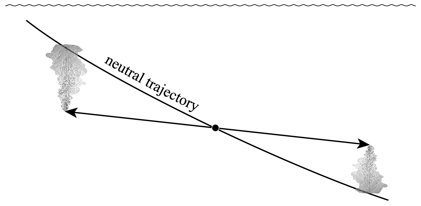
Figure 9 A sketch of what would be expected if lateral mixing did not occur along the neutral tangent plane (neutral trajectory). If a seawater parcel was moved adiabatically either left or right in a direction that was not neutral, it would find that it had a different specific volume to the ocean fluid at its new location. This difference would drive vertical motion, convection and turbulence.

Turbulent mixing is envisaged to occur in a two-stage process. First there is an advection stage where fluid parcels are moved (or exchanged) in an adiabatic and isentropic manner, followed by a second stage where diapycnal mixing (and intimate molecular diffusion) occurs. The same two-stage approach applies to lateral mixing along the neutral tangent plane. In the first stage a fluid parcel is moved a small distance to a new location where the infinitesimal change of pressure is δP while the Absolute Salinity and Conservative Temperature of this seawater parcel are unchanged (since these properties are both “potential” properties) so that the parcel's in-situ density has changed by ρκδP where κ is the adiabatic and isentropic compressibility, $\mathit{\kappa }=-v^{-\mathrm{1}}{\widehat{v}}_{\mathrm{P}}$, where the over-hat indicates that specific volume is being taken to be a function of $(S_{\mathrm{A}},\mathrm{\Theta },P)$. At this new location the ocean environment that surrounds the isolated parcel has an Absolute Salinity that is δS_A different to that at the original location and a Conservative Temperature that is different by δΘ. The in-situ density of the surrounding ocean at this new location is different to that at the original location by $\mathit{\rho }(\mathit{\kappa }\mathit{\delta }P+\mathit{\beta }\mathit{\delta }{S}_{\mathrm{A}}-\mathit{\alpha }\mathit{\delta }\mathrm{\Theta })$ where β and α are the saline contraction coefficient, $-v^{-\mathrm{1}}{\widehat{v}}_{S_{\mathrm{A}}}$, and thermal expansion coefficient, $v^{-\mathrm{1}}{\widehat{v}}_{\mathrm{\Theta }}$, respectively. As discussed in the previous paragraph, the key property of the neutral tangent plane is that seawater parcels do not experience Archimedean buoyant forces when moved small distances in a neutral direction and this requires that the in-situ density of our isolated seawater parcel is the same as the in-situ density of the surrounding ocean at this location, that is, $\mathit{\rho }\mathit{\kappa }\mathit{\delta }P=\mathit{\rho }(\mathit{\kappa }\mathit{\delta }P+\mathit{\beta }\mathit{\delta }{S}_{\mathrm{A}}-\mathit{\alpha }\mathit{\delta }\mathrm{\Theta })$. Hence along a neutral trajectory the variations of Absolute Salinity and Conservative Temperature must obey βδS_A=αδΘ, which applies to both spatial and temporal changes, so that in the limit we have the differential relationships (McDougall, 1987a)

$$\begin{array}{}\text{(39)}& \mathit{\alpha }{\mathrm{\nabla }}_n\mathrm{\Theta }=\mathit{\beta }{\mathrm{\nabla }}_n{S}_{\mathrm{A}},\text{ and }\mathit{\alpha }{\left.{\displaystyle \frac{\partial \mathrm{\Theta }}{\partial t}}\right|}_n=\mathit{\beta }{\left.{\displaystyle \frac{\partial S_{\mathrm{A}}}{\partial t}}\right|}_n,\end{array}$$

where ∇_n denotes the spatial gradient operator in the neutral tangent plane (see McDougall et al., 2014b for more details).

If the seawater parcel described above continues to not mix with its surroundings but instead retains its original Absolute Salinity and Conservative Temperature as it moves finite distances around the ocean (for example, as a sub-mesoscale coherent vortex, SCV) the property of “zero Archimedean buoyant force” for such a finite-amplitude lateral excursion is described by a zero value of the specific volume anomaly $\stackrel{\mathrm{̃}}{\mathit{\delta }}$ defined by (see McDougall, 2026)

$$\begin{array}{}\text{(40)}& \stackrel{\mathrm{̃}}{\mathit{\delta }}(S_{\mathrm{A}},\mathrm{\Theta },P)\equiv v(S_{\mathrm{A}},\mathrm{\Theta },P)-v\left({\stackrel{\mathrm{̃}}{S}}_{\mathrm{A}},\stackrel{\mathrm{̃}}{\mathrm{\Theta }},P\right).\end{array}$$

Such a seawater parcel with the constant values ${\stackrel{\mathrm{̃}}{S}}_{\mathrm{A}}$ and $\stackrel{\mathrm{̃}}{\mathrm{\Theta }}$ moves on the ocean's $\stackrel{\mathrm{̃}}{\mathit{\delta }}=\mathrm{0}$ surface, and this “SCV” behaviour has been discussed and quantified by McDougall (1987c) and Lang et al. (2020).

The gradient of $\stackrel{\mathrm{̃}}{\mathit{\delta }}$ in the neutral tangent plane (the epineutral gradient) can be shown to be (from Klocker et al., 2009, and McDougall and Klocker, 2010)

$$\begin{array}{}\text{(41)}& {\stackrel{\mathrm{̃}}{\mathit{\rho }}}^{\mathrm{\Theta }}{\mathrm{\nabla }}_n\stackrel{\mathrm{̃}}{\mathit{\delta }}\approx T_{\mathrm{b}}(\mathrm{\Theta }-\stackrel{\mathrm{̃}}{\mathrm{\Theta }}){\mathrm{\nabla }}_{n}P\end{array}$$

where ${\stackrel{\mathrm{̃}}{\mathit{\rho }}}^{\mathrm{\Theta }}$ is potential density referenced to the pressure $\stackrel{\mathrm{̃}}{P}$, T_b is the thermobaric parameter $T_{\mathrm{b}}\equiv {\widehat{\mathit{\alpha }}}_P-(\widehat{\mathit{\alpha }}/\widehat{\mathit{\beta }}){\widehat{\mathit{\beta }}}_P$ and again, the over-hats indicate that these variables are functions of ($S_{\mathrm{A}},\mathrm{\Theta },P$). The corresponding epineutral gradient of the potential density ${\stackrel{\mathrm{̃}}{\mathit{\rho }}}^{\mathrm{\Theta }}$ is (from McDougall, 1987a)

$$\begin{array}{}\text{(42)}& {\mathrm{\nabla }}_n\ln {\stackrel{\mathrm{̃}}{\mathit{\rho }}}^{\mathrm{\Theta }}\approx T_{\mathrm{b}}(P-\stackrel{\mathrm{̃}}{P}){\mathrm{\nabla }}_n\mathrm{\Theta },\end{array}$$

while from Appendix A of McDougall et al. (2017) we have the following expression for the gradient of ${\stackrel{\mathrm{̃}}{\mathit{\rho }}}^{\mathrm{\Theta }}$ in a $\stackrel{\mathrm{̃}}{\mathit{\delta }}$ surface,

$$\begin{array}{}\text{(43)}& {\mathrm{\nabla }}_{\stackrel{\mathrm{̃}}{\mathit{\delta }}}\ln {\stackrel{\mathrm{̃}}{\mathit{\rho }}}^{\mathrm{\Theta }}\approx T_{\mathrm{b}}{\mathrm{\nabla }}_{\stackrel{\mathrm{̃}}{\mathit{\delta }}}\left[\right(P-\stackrel{\mathrm{̃}}{P}\left)\right(\mathrm{\Theta }-\stackrel{\mathrm{̃}}{\mathrm{\Theta }}\left)\right],\end{array}$$

where ∇_nΘ and ∇_nP have been assumed to be approximately parallel to each other. The important message from Eqs. (41) and (42) is that both ${\stackrel{\mathrm{̃}}{\mathit{\rho }}}^{\mathrm{\Theta }}$ and $\stackrel{\mathrm{̃}}{\mathit{\delta }}$ vary quadratically in space as one moves along a neutral trajectory away from the original location where the ocean properties are (${\stackrel{\mathrm{̃}}{S}}_{\mathrm{A}},\stackrel{\mathrm{̃}}{\mathrm{\Theta }},\stackrel{\mathrm{̃}}{P}$), while from Eq. (43) we glean that the originally referenced potential density ${\stackrel{\mathrm{̃}}{\mathit{\rho }}}^{\mathrm{\Theta }}$ varies quadratically with distance along the $\stackrel{\mathrm{̃}}{\mathit{\delta }}$ specific volume anomaly surface, this being the surface along which adiabatically insulated fluid parcels move. Hence as the limit of a small horizontal displacement is taken, the $\stackrel{\mathrm{̃}}{\mathit{\delta }}$ surface and the ${\stackrel{\mathrm{̃}}{\mathit{\rho }}}^{\mathrm{\Theta }}$ surface coincide (osculate) with the neutral tangent plane.

The slope of the neutral tangent plane can be compared to the slopes of other surfaces such as potential density surfaces and specific volume anomaly surfaces using simple formulae available in McDougall (1987a, c, 1989) and McDougall and Jackett (1988). An interesting case is the surface of constant in-situ density ρ because incompressible ocean floats move on such surfaces since both their mass and their volume are constant. These surfaces are close to being isobaric surfaces when the vertical stratification is weak, such that even at a depth of 1000 m, in-situ density surfaces typically have a slope of only 20 % of the slope of the neutral tangent plane (McDougall, 1989).

There have been three suggested theoretical alternatives to the neutral direction as the direction in which the strong lateral mixing of mesoscale eddies might be directed. The first (chronologically) is the orthobaric surface concept of de Szoeke et al. (2000), the second is the P-vector (minimum energy direction) concept of Nycander (2011), and the third is the suggestion of Tailleux (2016a, b) that a neutral surface should be a function of only Absolute Salinity and Conservative Temperature, γ(S_A,Θ). We discuss these suggestions in the following three paragraphs in the chronological order of their publication.

A variable called orthobaric density was introduced by de Szoeke et al. (2000). Orthobaric density ρ_v(ρ,P) is a function of only in-situ density and pressure, and McDougall and Jackett (2005b) showed that while it is possible to derive a function of this form to be relatively neutral at all depths in a single ocean basin, it is not possible to do so in both hemispheres because different ρ_v(ρ,P) branches exist on either side of the maximum pressure on a neutral surface. One way of seeing this problem with ρ_v(ρ,P) is from Eq. (42) above. As one proceeds along a neutral path from the outcrop in the South Atlantic to the outcrop in the North Atlantic, the Conservative Temperature increases as does the potential density (referenced to the sea surface) and on some surfaces this increase of potential density exceeds 0.1 kg m⁻³. This explains why the “patched isopycnals” of Reid (1994) had the potential density of the northern and Southern Hemisphere outcrops of the same “patched isopycnal” surface being different by ∼ 0.1 kg m⁻³. At the two outcrops of a neutral surface in the different hemispheres the pressures are the same, but the in-situ densities are different by 0.1 kg m⁻³, hence a neutral surface cannot be described by a single-valued function ρ_v(ρ,P). The two different branches of ρ_v(ρ,P) functions bifurcate near the equator where the epineutral gradient of pressure is zero (see McDougall and Jackett, 2005b).

Nycander (2011) studied mixing in the ocean along inclined planes and sought a direction in which a pair of parcels could exchange positions “without encountering a force” (neither a vertical nor a horizontal force), so not require any energy to exchange the parcels. However the direction of Nycander's P vector depends on an unknown reference pressure in the expression for dynamic enthalpy, and so the direction of the P-vector cannot be determined. However, if this reference pressure is taken to be the in-situ pressure of the parcel exchange, then the P surface coincides with the neutral tangent plane. We ask, when considering an individual mixing event, why would any pressure other than the in-situ pressure of the mixing event be relevant? Because Nycander's approach did not lead to a conclusion as to the direction of lateral mixing in the ocean we interpret this as further support for the long-standing practice (since the 1980s) of defining the neutral direction in terms of the lack of vertical Archimedean buoyant forces, rather than in terms of the changes in gravitational potential energy, or indeed, of any other type of energy. The P-vector idea pursued by Nycander (2011) lacks a physical theorem or principle that motivates energetic minimisation as a desirable property to pursue, and in any case, it has not led to a conclusion because there is no guidance as to what the reference pressure of the potential energy might be. Admittedly the definition of the neutral tangent plane in terms of the lack of Archimedean buoyant forces also lacks a motivating fundamental theorem or principle: instead, it has observational support from the measurements of weak diapycnal mixing in the ocean interior. Since we have discussed gravitational potential energy (GPE) in this paragraph it is worth mentioning the concept of available potential energy (APE) which is defined as that part of the GPE of the global ocean that exceeds that of a resting ocean in which all density surfaces coincide with geopotential surfaces. This resting state is often called the Lorenz-levelled reference state. This reference state has traditionally been difficult to find because of the nonlinear nature of the equation of state of seawater, but Saenz et al. (2015) have pioneered a method that is able to find this state in a computationally efficient manner.

Tailleux (2016a, b) also discuss the mixing by mesoscale eddies and propose that the surface on which this strong mixing occurs is a quasi-material surface, that is, a surface defined by a constant value of a single-valued function γ(S_A,Θ) of only Absolute Salinity and Conservative Temperature fitted to the existing water masses in the global ocean. Such a globally defined function is not consistent with the physics of baroclinic instability which depends on the ocean properties in the region of the instability; the physics of a local mixing event should not depend on the nature of the water masses in a distant ocean basin in a different hemisphere. The reason why a function of the form γ(S_A,Θ) cannot be neutral in the global ocean can be understood from the neutral relationship of Eq. (39), namely α∇_nΘ=β∇_nS_A. As one proceeds along a neutral trajectory from the outcrop in the South Atlantic towards the outcrop in the North Atlantic, the Conservative Temperature and Absolute Salinity increase until they both reach maxima at the approximate latitude of the Mediterranean Sea. Proceeding northwards along the neutral trajectory from this location, the Conservative Temperature and Absolute Salinity now decrease, but the locus of these points on the (S_A,Θ) diagram do not overly the locus of points along the initial trajectory from the southern outcrop to the middle latitudes of the North Atlantic. These sets of points do not overlap because the ratio $\mathit{\alpha }/\mathit{\beta }$ depends on pressure, and the pressure of the data on the neutral trajectory north of the Mediterranean latitude at a given Conservative Temperature, is different to the pressure at the corresponding Conservative Temperature on the southern part of the neutral trajectory. The result is that at a given Conservative Temperature on the same neutral trajectory there are multiple value of Absolute Salinity, as is illustrated in Fig. 9(a) of McDougall and Jackett (2007) for the hydrography of the Atlantic. This means that data on a neutral trajectory, or on an approximately neutral surface, cannot be fitted with a single-valued function γ(S_A,Θ) nor indeed with a single-valued function of the form $\mathit{\gamma }(S_{\mathrm{A}},\mathrm{\Theta },P)$; see Fig. 10 of McDougall and Jackett (2007). This effect can occur even when neutral helicity is zero everywhere. Note that the multi-valued nature of a function γ(S_A,Θ) that would be needed to fit such an approximately neutral surface does not imply that there is path-dependent induced dianeutral upwelling through the approximately neutral surface (McDougall and Jackett, 2007). A more detailed explanation of the reasons for the non-neutrality of the γ(S_A,Θ) functional form can be found in McDougall and Jackett (2005b, 2007).

11 Thermobaricity and Cabbeling

Neglecting the non-conservative source terms (including the term in the dissipation of turbulent kinetic energy, $\mathit{\epsilon }/{\widehat{h}}_{\mathrm{\Theta }}$), the evolution equation (33) for Conservative Temperature becomes (with D and K being the small-scale isotropic and the epineutral scalar diffusivities, respectively)

$$\begin{array}{}\text{(44)}& \begin{array}{rl}{\left.{\displaystyle \frac{\partial \mathrm{\Theta }}{\partial t}}\right|}_n+\mathit{v}\cdot {\mathrm{\nabla }}_n\mathrm{\Theta }+e{\displaystyle \frac{\partial \mathrm{\Theta }}{\partial z}}=& {\mathit{\gamma }}_z{\mathrm{\nabla }}_n\cdot \left({\mathit{\gamma }}_z^{-\mathrm{1}}K{\mathrm{\nabla }}_n\mathrm{\Theta }\right)\\ & +(D{\mathrm{\Theta }}_z{)}_z,\end{array}\end{array}$$

where v is the thickness-weighted horizontal velocity of density-coordinate averaging, or equivalently the horizontal Temporal-Residual-Mean (TRM) velocity, e is the mean vertical velocity through the locally referenced potential density surface, and Θ is the thickness-weighted Conservative Temperature obtained by temporal averaging in Neutral Density coordinates. The terms in the vertical gradient of locally referenced potential density, γ_z, and its reciprocal, account for the lateral gradient of the thickness between density surfaces along which the lateral diffusivity K acts. The lateral gradient operator ∇_n measures the lateral variations of properties in the locally referenced potential density surface which osculates with the neutral tangent plane. The averaging procedure to obtain this TRM-mean evolution equation was derived by McDougall and McIntosh (2001) and is also explained in Sect. A21 of the TEOS-10 Manual (IOC et al., 2010). The corresponding evolution equation for Absolute Salinity is (also ignoring the biogeochemical source term of Absolute Salinity, which for large-scale oceanography, is not insignificant)

$$\begin{array}{}\text{(45)}& \begin{array}{rl}{\left.{\displaystyle \frac{\partial S_{\mathrm{A}}}{\partial t}}\right|}_n+\mathit{v}\cdot {\mathrm{\nabla }}_n{S}_{\mathrm{A}}+e{\displaystyle \frac{\partial S_{\mathrm{A}}}{\partial z}}=& {\mathit{\gamma }}_z{\mathrm{\nabla }}_n\cdot \left({\mathit{\gamma }}_z^{-\mathrm{1}}K{\mathrm{\nabla }}_n{S}_{\mathrm{A}}\right)\\ & +(D{S}_{{\mathrm{A}}_z}{)}_z.\end{array}\end{array}$$

It is instructive to take two different linear combinations of these evolution equations for Θ and S_A with the first combination chosen to eliminate the dianeutral velocity e, and the second to eliminate the temporal and lateral advection terms (using the temporal and spatial neutral relationships Eq. 39), leading to the following two equations (where the cabbeling coefficient is defined by $C_{\mathrm{b}}\equiv {\widehat{\mathit{\alpha }}}_{\mathrm{\Theta }}+\mathrm{2}(\widehat{\mathit{\alpha }}/\widehat{\mathit{\beta }}){\widehat{\mathit{\alpha }}}_{S_{\mathrm{A}}}-(\widehat{\mathit{\alpha }}/\widehat{\mathit{\beta }}{)}^{\mathrm{2}}{\widehat{\mathit{\beta }}}_{S_{\mathrm{A}}}$ and, as a reminder, the over-hats indicate that these variables are functions of ($S_{\mathrm{A}},\mathrm{\Theta },P)$).

$$\begin{array}{}\text{(46)}& \begin{array}{rl}{\left.{\displaystyle \frac{\partial \mathrm{\Theta }}{\partial t}}\right|}_n+\mathit{v}\cdot {\mathrm{\nabla }}_n\mathrm{\Theta }=& {\mathit{\gamma }}_z{\mathrm{\nabla }}_n\cdot \left({\mathit{\gamma }}_z^{-\mathrm{1}}K{\mathrm{\nabla }}_n\mathrm{\Theta }\right)\\ & +Kg{N}^{-\mathrm{2}}{\mathrm{\Theta }}_z(C_{\mathrm{b}}{\mathrm{\nabla }}_n\mathrm{\Theta }\cdot {\mathrm{\nabla }}_n\mathrm{\Theta }\\ & +T_{\mathrm{b}}{\mathrm{\nabla }}_n\mathrm{\Theta }\cdot {\mathrm{\nabla }}_{n}P)\\ & +D\mathit{\beta }g{N}^{-\mathrm{2}}{\mathrm{\Theta }}_z^{\mathrm{3}}{\displaystyle \frac{d^{\mathrm{2}}{S}_{\mathrm{A}}}{d{\mathrm{\Theta }}^{\mathrm{2}}}},\end{array}\end{array}$$

and

$$\begin{array}{}\text{(47)}& \begin{array}{rl}e{g}^{-\mathrm{1}}{N}^{\mathrm{2}}=& -K(C_{\mathrm{b}}{\mathrm{\nabla }}_n\mathrm{\Theta }\cdot {\mathrm{\nabla }}_n\mathrm{\Theta }+T_{\mathrm{b}}{\mathrm{\nabla }}_n\mathrm{\Theta }\cdot {\mathrm{\nabla }}_{n}P)\\ & +\mathit{\alpha }(D{\mathrm{\Theta }}_z{)}_z-\mathit{\beta }(D{S}_{{\mathrm{A}}_z}{)}_z.\end{array}\end{array}$$

These equations were derived by McDougall (1987a, b) and a discussion of them can also be found in Sects. A22 and A23 of IOC et al. (2010). Equation (47) shows that the dianeutral velocity is not a separate physical process but rather is a consequence of the processes of lateral and small-scale isotropic mixing as parameterized with the diffusivities K and D.

When the dianeutral velocity is eliminated from Eqs. (44) and (45) to obtain Eq. (46) one finds that the small-scale mixing process, D, only affects epineutral changes (in time and/or space) in proportion to the curvature $d^{\mathrm{2}}{S}_{\mathrm{A}}/d{\mathrm{\Theta }}^{\mathrm{2}}$ of the vertical water column on the S_A−Θ diagram. In the other case, when the epineutral gradients are eliminated, one finds in Eq. (47) that the dianeutral velocity is caused not only by the small-scale isotropic mixing process but also by $-K(C_{\mathrm{b}}{\mathrm{\nabla }}_n\mathrm{\Theta }\cdot {\mathrm{\nabla }}_n\mathrm{\Theta }+T_{\mathrm{b}}{\mathrm{\nabla }}_n\mathrm{\Theta }\cdot {\mathrm{\nabla }}_{n}P)$ where the epineutral mixing acts in conjunction with the nonlinear nature of the equation of state, resulting in two contributions, cabbeling and thermobaricity, to dianeutral advection.

The thermobaricity and cabbeling processes can be understood with the aid of Fig. 10. Epineutral mixing involves first the movement of fluid parcels in an adiabatic and isentropic manner, followed by the intimate mixing between them. During the adiabatic and isohaline movements the two seawater parcels move along specific volume anomaly surfaces (see the discussion at the beginning of Sect. 10 above). Consider two fluid parcels labelled A and B in Fig. 10a that have been chosen because they get to meet and mix subsequently at physical location D. Parcels A and B were originally on a neutral trajectory along which there are variations of pressure (slope) and Conservative Temperature, and as parcel A is moved to the right, its constant value of Conservative Temperature is soon less than that on the neutral trajectory. This means that the insulated parcel A has a larger compressibility than the fluid surrounding it, and as it moves further to the right it sinks to be further separated from the neutral trajectory. This can be seen in Eq. (41): the insulated parcel A has a constant (zero) value of $\stackrel{\mathrm{̃}}{\mathit{\delta }}$, but the value of $\stackrel{\mathrm{̃}}{\mathit{\delta }}$ on the neutral trajectory increases quadratically to the right from the original location A. The opposite thing happens to parcel B, and the two parcels A and B soon meet at a location where the ocean's properties have properties D. The vertical movement of parcels A and B through the neutral trajectory is called thermobaricity and is due to the thermobaric nonlinearity of the equation of state as reflected in the thermobaric parameter $T_{\mathrm{b}}\equiv {\widehat{\mathit{\alpha }}}_P-(\widehat{\mathit{\alpha }}/\widehat{\mathit{\beta }}){\widehat{\mathit{\beta }}}_P$. Up to this point in the process no intimate mixing has occurred, and in principle, the movements could be reversed. Upon mixing, the density of the mixed fluid is increased so that the potential density referenced to the pressure of parcel D increases and the mixture has properties E (on Fig. 10b) and sinks to location E on Fig. 10a. This part of the process is called cabbeling, and the intimate mixing has also made the dianeutral advection of thermobaricity irreversible (permanent).

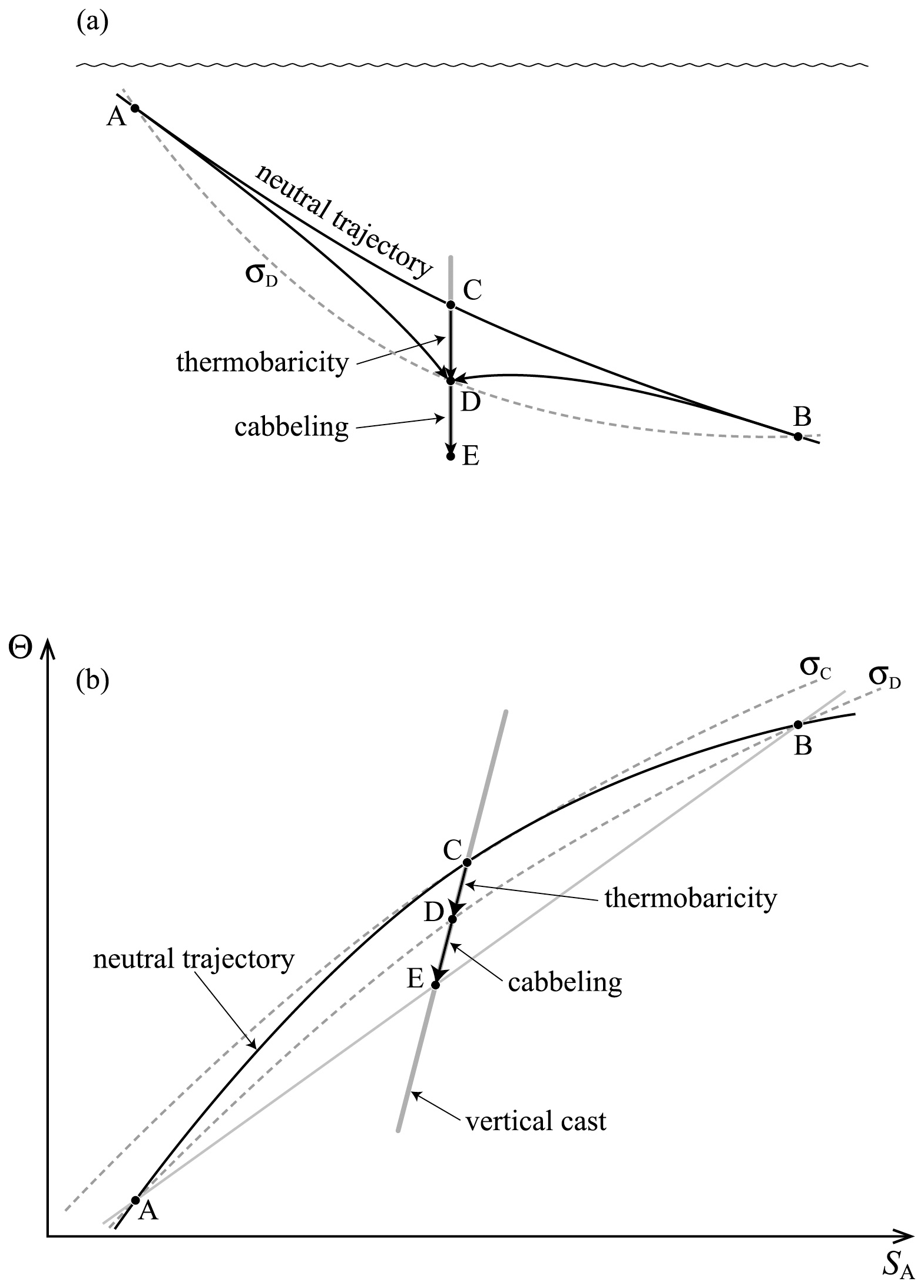
Figure 10 A sketch used to describe the thermobaricity and cabbeling processes in (a) a vertical cross-section, and (b) on the salinity-temperature diagram.

Figure 10 is an explanation of the thermobaricity and cabbeling processes based on the advection and mixing of two fluid parcels. Klocker and McDougall (2010a) have shown that the total dianeutral transport due to cabbeling and thermobaricity (in Sverdups per unit length along the front) across an oceanic epineutral front (that is, a location where there is a gradient of Conservative Temperature on the neutral tangent plane) can be quantified in terms of the product of the average epineutral flux of temperature −K∇_nΘ in the frontal region and the total epineutral differences of Conservative Temperature and of pressure, respectively, across the front. In this way the area-integrated effects of thermobaricity and cabbeling do not depend on having to estimate the epineutral property gradients such as ∇_nΘ, or the epineutral diffusivity K, but rather depend on the spatially averaged epineutral heat flux, and the total cross-frontal epineutral temperature and pressure differences. Several studies such as McDougall and You (1990), McDougall (1991), Iudicone et al. (2008), Klocker and McDougall (2010a), Groeskamp et al. (2016) and Groeskamp (2026) have quantified the magnitudes of thermobaricity and cabbeling in the global ocean and have shown that they are the dominant cause of dianeutral advection in the interior of the Southern Ocean. Moreover, the several Sverdrups of dianeutral advection of thermobaricity and cabbeling in the Southern Ocean are negative (that is, downwards) thus requiring the upwelling caused by small-scale turbulent mixing to be larger than would otherwise be the case.

12 Neutral helicity and the ill-defined nature of neutral surfaces

Equation (39) above defines the neutral tangent plane in terms of the compensating gradients of Absolute Salinity and Conservative Temperature, $\mathit{\alpha }{\mathrm{\nabla }}_n\mathrm{\Theta }-\mathit{\beta }{\mathrm{\nabla }}_n{S}_{\mathrm{A}}=\mathrm{0}$, or equivalently, $\mathit{\kappa }{\mathrm{\nabla }}_{n}P-{\mathrm{\nabla }}_n\ln \mathit{\rho }=\mathrm{0}$, where κ is the adiabatic and isentropic compressibility. The neutral tangent plane can be found at each point in the ocean, but does this guarantee that these neutral tangent planes can be linked together to find a well-defined surface? Let us begin by assuming that these well-defined neutral surfaces do exist. In that case the integral along a series on neutral tangent planes around any closed path in longitude-latitude space will arrive back at the start at the same height as at the beginning of the loop. This means that the closed integral of Absolute Salinity around a loop in the surface is zero, that is, $\oint d{S}_{\mathrm{A}}=\mathrm{0}$, and it follows from Eq. (39) that the closed integral around the same loop along the neutral tangent planes, $\oint (\mathit{\alpha }/\mathit{\beta })d\mathrm{\Theta }$, must also be zero. If $\mathit{\alpha }/\mathit{\beta }$ were a function only of salinity and temperature (which it is not), then $\oint (\mathit{\alpha }/\mathit{\beta })d\mathrm{\Theta }$ would always be zero, but since $\mathit{\alpha }/\mathit{\beta }$ is also a function of pressure, this closed integral will not in general be zero; we will see below that this integral is only zero if the neutral helicity is zero, implying a very special relationship between pressure, salinity and temperature. Figure 1 of McDougall and Jackett (1988) illustrates how the pressure dependence of $\mathit{\alpha }/\mathit{\beta }$ can cause neutral surfaces to be ill-defined.

Here we explain the ill-defined nature of neutral surfaces by examining the property needed of the normal to the neutral tangent plane in order for a neutral surface to be well-defined. The (three dimensional) normal to the neutral tangent plane is in the direction $\mathit{\alpha }\mathrm{\nabla }\mathrm{\Theta }-\mathit{\beta }\mathrm{\nabla }{S}_{\mathrm{A}}=\mathit{\kappa }\mathrm{\nabla }P-\mathrm{\nabla }\ln \mathit{\rho }$ whose vertical component has magnitude g⁻¹N². The neutral tangent plane and its normal, α∇Θ−β∇S_A, exist at every point in space and one might think that this is sufficient to ensure that all the little tangent planes would join up to become a well-defined surface. But this is not the case. Rather, it can be shown (McDougall and Jackett, 1988, 2007) that the scalar product of the normal α∇Θ−β∇S_A with its curl being zero everywhere is a necessary condition for all the neutral tangent planes to join up and describe a surface. This triple scalar product is called the neutral helicity, H,

$$\begin{array}{}\text{(48)}& \begin{array}{rl}H& \equiv (\mathit{\alpha }\mathrm{\nabla }\mathrm{\Theta }-\mathit{\beta }\mathrm{\nabla }{S}_{\mathrm{A}})\cdot \mathrm{\nabla }\times (\mathit{\alpha }\mathrm{\nabla }\mathrm{\Theta }-\mathit{\beta }\mathrm{\nabla }{S}_{\mathrm{A}})\\ & =\mathit{\beta }{T}_{\mathrm{b}}\mathrm{\nabla }P\cdot \mathrm{\nabla }{S}_{\mathrm{A}}\times \mathrm{\nabla }\mathrm{\Theta }\\ & =g^{-\mathrm{1}}{N}^{\mathrm{2}}{T}_{\mathrm{b}}{\mathrm{\nabla }}_{n}P\times {\mathrm{\nabla }}_n\mathrm{\Theta }\cdot \mathit{k}\\ & =P_z\mathit{\beta }{T}_{\mathrm{b}}{\mathrm{\nabla }}_p{S}_{\mathrm{A}}\times {\mathrm{\nabla }}_p\mathrm{\Theta }\cdot \mathit{k}.\end{array}\end{array}$$

A zero value of neutral helicity everywhere on a surface is a necessary but not sufficient condition for neutral surfaces to exist because of the ability of islands to effectively “hide” neutral helicity but still cause path dependence; see the paragraph below that alludes to the work of Stanley (2019a) on this subject.

The last three parts of Eq. (48) have been found by expanding the definition of H in the first line, and k is the unit vertical vector. Each of these expressions contain the thermobaric parameter $T_{\mathrm{b}}\equiv {\mathit{\alpha }}_P-(\mathit{\alpha }/\mathit{\beta }){\mathit{\beta }}_P=\mathit{\beta }(\mathit{\alpha }/\mathit{\beta }{)}_P$ which again says that a prerequisite for a non-zero neutral helicity is that $\mathit{\alpha }/\mathit{\beta }$ be a function of pressure. We can discuss this equation in relation to Fig. 11. First, we know from the definition of the neutral tangent plane definition that $\mathit{\alpha }{\mathrm{\nabla }}_n\mathrm{\Theta }-\mathit{\beta }{\mathrm{\nabla }}_n{S}_{\mathrm{A}}=\mathrm{0}$ so that the neutral tangent plane must contain the line of constant temperature and salinity, ∇Θ×∇S_A. Similarly, we know that $\mathit{\kappa }{\mathrm{\nabla }}_{n}P-{\mathrm{\nabla }}_n\ln \mathit{\rho }=\mathrm{0}$ so the neutral tangent plane must also contain the line ∇P×∇ρ. Figure 11 shows the lines ∇Θ×∇S_A and ∇P×∇ρ, the neutral tangent plane (in red) and five other coloured planes.

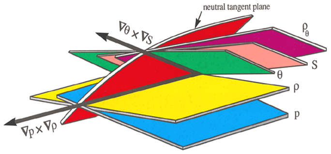
Figure 11 A sketch showing various planes of constant properties in three-dimensional space ($x,y,z)$ in the vicinity of a given point in the ocean. The neutral tangent plane contains both the lines ∇P×∇ρ and ∇Θ×∇S_A. While the neutral tangent plane exists everywhere in space, these little planes do not link up to form a well-defined neutral surface unless the neutral helicity is zero everywhere. This requires that the two lines ∇P×∇ρ and ∇Θ×∇S_A coincide.

The second line of Eq. (48), $H=\mathit{\beta }{T}_{\mathrm{b}}\mathrm{\nabla }P\cdot \mathrm{\nabla }{S}_{\mathrm{A}}\times \mathrm{\nabla }\mathrm{\Theta }$, can be understood from Fig. 11 as requiring that if H is to be zero ∇Θ×∇S_A must lie in the plane of constant pressure; approximately we can say that ∇Θ×∇S_A must be a horizontal vector with no vertical component. It seems rather coincidental that this should be the case in general in the ocean. Now expanding ∇ρ in terms of gradients of salinity, temperature and pressure it can be shown that if neutral helicity H is to be zero then the two lines ∇Θ×∇S_A and ∇P×∇ρ must coincide. The third line of Eq. (48) says that the two-dimensional gradients of pressure and temperature in the neutral tangent plane must be parallel to each other if neutral helicity is to be zero. The fourth line of Eq. (48) says that the two-dimensional gradients of salinity and temperature in the pressure surface must be parallel to each other if neutral helicity is to be zero. Each of these constraints that result from a requirement that neutral helicity be zero seem quite restrictive, but it turns out that most of the ocean has small values of neutral helicity, with the epineutral gradients of pressure and temperature, ∇_nP and ∇_nΘ usually being close to parallel, and when they are not close to parallel, at least one of them has small magnitude. Each of these geometrical interpretations of neutral helicity have been explored and illustrated with oceanographic data in McDougall and Jackett (1988, 2007).

Stanley (2019a) has shown that it is possible for a neutral trajectory to exhibit a vertical excursion after completing a closed loop in latitude and longitude even if the neutral helicity is zero everywhere in the ocean. This occurs when the loop encloses land (an island, or a seamount) inside of which the neutral helicity can effectively “hide”. In this situation the neutral helicity can be zero everywhere along the neutral trajectory, and indeed throughout the entire ocean, but the neutral surface still does not exist. This example of path-dependence was missed in the earlier studies by McDougall and coauthors.

Note that neutral helicity can be expressed in terms of the thermal wind (the vertical gradient of the Eulerian mean geostrophic horizontal velocity $\stackrel{\mathrm{‾}}{v}$) by

$$\begin{array}{}\text{(49)}& H=\mathit{\rho }{T}_{\mathrm{b}}f{\stackrel{\mathrm{‾}}{\mathit{v}}}_z\cdot {\mathrm{\nabla }}_n\mathrm{\Theta },\end{array}$$

showing that neutral helicity is proportional to the component of the thermal wind, ${\stackrel{\mathrm{‾}}{\mathit{v}}}_z$, in the direction of the epineutral temperature gradient, ∇_nΘ (Sect. 3.13 of IOC et al., 2010).

The same geometrical combination of two-dimensional temperature (or salinity) and pressure gradients, ${\mathrm{\nabla }}_{n}P\times {\mathrm{\nabla }}_n\mathrm{\Theta }\cdot \mathit{k}$, that appears in the expression for neutral helicity also occurs in the expression for the mean absolute velocity in terms of the ocean's hydrography. However, in this case the thermobaric coefficient does not multiply ${\mathrm{\nabla }}_{n}P\times {\mathrm{\nabla }}_n\mathrm{\Theta }\cdot \mathit{k}$. The geostrophic balance can be exploited to find the following expression for the mean Eulerian velocity $\stackrel{\mathrm{‾}}{\mathit{v}}$ (as opposed to the temporal residual-mean velocity v in Eq. 46)

$$\begin{array}{}\text{(50)}& \stackrel{\mathrm{‾}}{\mathit{v}}=\left\{{\displaystyle \frac{N^{\mathrm{2}}}{fg\mathit{\rho }}}{\displaystyle \frac{{\mathrm{\nabla }}_{n}P\times \mathit{\tau }\cdot \mathit{k}}{{\mathit{\varphi }}_z}}-{\displaystyle \frac{v_z^{\perp }}{{\mathit{\varphi }}_z}}\right\}\mathit{\tau }\times \mathbf{k}+v^{\perp }\mathit{\tau },\end{array}$$

(McDougall, 1995 and Sect. 3.13 of IOC et al., 2010) where τ is the unit epineutral temperature gradient vector, ${\mathrm{\nabla }}_n\mathrm{\Theta }/\mathrm{|}{\mathrm{\nabla }}_n\mathrm{\Theta }\mathrm{|}$, ϕ_z is the rate at which the direction of ∇_nΘ changes in the vertical (in radians m⁻¹) and v^⊥ is the component of $\stackrel{\mathrm{‾}}{\mathit{v}}$ in the τ direction; this component being caused by mixing processes (as in Eq. 3.13.7 of IOC et al., 2010). Estimates of the absolute velocity usually come from performing an inverse study, and in fact Eq. (50) is the result of such an inverse method since it uses the geostrophic balance equation at two heights separated by the infinitesimal distance dz in the vertical. Equation (50) implies that neutral helicity needs to be non-zero in order for the ocean to have mean Eulerian motion (apart the mean velocity v^⊥τ caused by mixing processes). The study of Eq. (50) for understanding the mean circulation in the ocean has not really begun, but in any case, the ocean seems able to satisfy this requirement while having what seems like small neutral helicity in most places (see the following Sect. 12.1).

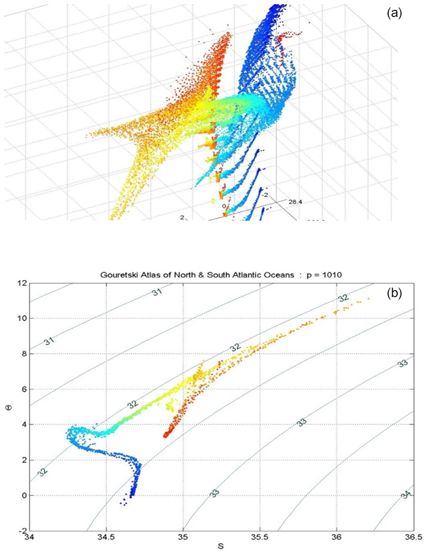
Figure 12 (a) A view of the South and North Atlantic hydrographic data in three-dimensional ($S_{\mathrm{A}},\mathrm{\Theta },P$) space. (b) A section through the same ($S_{\mathrm{A}},\mathrm{\Theta },P$) data at a pressure of 1010 dbar.

12.1 The ocean is quite empty in salinity-temperature-pressure space

Here we begin by exploring what constraint there might be on the ocean hydrography if neutral helicity $\mathrm{\nabla }P\cdot \mathrm{\nabla }{S}_{\mathrm{A}}\times \mathrm{\nabla }\mathrm{\Theta }$ were zero everywhere in the ocean. It can be shown that if $P(x,y,z)$, $S_{\mathrm{A}}(x,y,z)$ and $\mathrm{\Theta }(x,y,z)$ everywhere obey $\mathrm{\nabla }P\cdot \mathrm{\nabla }{S}_{\mathrm{A}}\times \mathrm{\nabla }\mathrm{\Theta }=\mathrm{0}$, then all the pressure, salinity and temperature data lie on a single surface in $S_{\mathrm{A}}-\mathrm{\Theta }-P$ space (McDougall and Jackett, 2007). This theoretical result prompted the visualization of the salinity-temperature-pressure data of the global ocean by rotating this ocean hydrograhic data in $S_{\mathrm{A}}-\mathrm{\Theta }-P$ space. This rotating visualization revealed that the global ocean is rather “empty” or “hollow” in this space, as is illustrated in Fig. 12.

Figure 12a shows a particular view in $S_{\mathrm{A}}-\mathrm{\Theta }-P$ space of all the hydrography of the South and North Atlantic oceans. The blue data from the South Atlantic is clearly separated from the North Atlantic data in red. It is much more obvious to see that the data lies close to a single surface when viewing the data as it rotates in $S_{\mathrm{A}}-\mathrm{\Theta }-P$ space on a computer screen, thereby viewing the data from many different angles. Another way of making this point is to display the hydrographic data on the two-dimensional S_A−Θ plot at just one pressure, and an example is shown in Fig. 12b. This two-dimensional cut through the three-dimensional $S_{\mathrm{A}}-\mathrm{\Theta }-P$ data clearly demonstrates the emptiness of the ocean's hydrography in $S_{\mathrm{A}}-\mathrm{\Theta }-P$ space. At the pressure of 1010 dbar (Fig. 12b) the data snakes around on the S_A−Θ diagram with the warmest and saltiest data being the signature of Mediterranean Water in the North Atlantic. If the data fell exactly on a single curved line, the neutral helicity would be exactly zero everywhere at this pressure (see the last line of Eq. 48) and neutral surfaces would be well-defined in this vicinity. This is not totally the case, but the data of Fig. 12b fills only a few percent of the smallest area defined so that every data point can be connected to every other data point by straight lines that lie wholly within the area. It is not immediately obvious whether filling out only a few percent of such an area represents a very small amount of neutral helicity or not, but the next section attempts to address this question by concentrating on the consequences of (i) the mean vertical advection that occurs because the lateral flow is forced to move along an approximately neutral surface rather than along the neutral tangent plane, and (ii) having lateral mixing occurring along surfaces that differ from the neutral tangent plane.

12.2 Approximately neutral surfaces

There are many different types of surfaces that have been designed with the aim of being approximately neutral. Examples are potential density surfaces, patched potential density surfaces (Reid, 1994), Neutral Density surfaces (Jackett and McDougall, 1997), and some of the purpose-built algorithms specifically designed to approximate neutrality, which we now describe. The Neutral Density algorithm operates by neutrally relating a given hydrographic observation to a pre-labelled global atlas, thus giving the observation a Neutral Density value. Having labelled a data set with Neutral Density, an iso-surface of Neutral Density can then be formed. The Neutral Density algorithm has not yet been updated from EOS-80 to TEOS-10, nor does it yet operate north of 60° N in the North Atlantic. Fixing these deficiencies requires a new labelled reference data set of neutral density values in a global atlas that extends into the Arctic Ocean, a task that has not been completed.

Another type of approximately neutral surface is called an “ω surface” (Klocker et al., 2009) which is formed iteratively from an initial surface that could be a potential density surface or even an isobaric surface. In this initial surface the gradients of Absolute Salinity and Conservative Temperature do not completely compensate each other in terms of their effects of density. That is, $\mathit{\alpha }{\mathrm{\nabla }}_a\mathrm{\Theta }-\mathit{\beta }{\mathrm{\nabla }}_a{S}_{\mathrm{A}}\ne \mathrm{0}$, in comparison with the neutral tangent plane in which α∇_nΘ−β∇_nS_A is zero. The method works using a two-step iterative procedure. In the first step the scalar function of longitude and latitude Φ(x,y) is found that minimizes the integral of

$$\begin{array}{}\text{(51)}& (\mathit{\alpha }{\mathrm{\nabla }}_a\mathrm{\Theta }-\mathit{\beta }{\mathrm{\nabla }}_a{S}_{\mathrm{A}}+{\mathrm{\nabla }}_a\mathrm{\Phi })\cdot (\mathit{\alpha }{\mathrm{\nabla }}_a\mathrm{\Theta }-\mathit{\beta }{\mathrm{\nabla }}_a{S}_{\mathrm{A}}+{\mathrm{\nabla }}_a\mathrm{\Phi }),\end{array}$$

over the area of the initial surface. Φ(x,y) is then interpreted as an increment of the natural logarithm of locally referenced potential density and the second step converts Φ(x,y) to a height increment using a linear Newton step based on the local stratification. The height of the updated surface is then taken to be the original height of the surface plus this height increment. The two-step process is then repeated with this updated surface as the initial condition. Stanley et al. (2021) have made this process computationally efficient by accurately finding the increment of height on the (x,y) vertical cast corresponding to the same increment Φ(x,y) in ln ρ^l, and then using a Poisson equation solver in two dimensions. Their method converges to the final ω surface in the global ocean after just two or three iterations after starting with a potential density surface, and the method includes the “wetting” at new (x,y) locations as each successive iteration adjusts the height of the surface and hence its ability to talk neutrally to adjacent locations.

Lang et al. (2023) have presented additional variations of the ω surface methodology by minimizing not only the gradient of locally referenced potential density in the final approximately neutral ω surface but also the component of the three-dimensional velocity vector through the final surface due to it not exactly coinciding with the neutral tangent plane. This method needs knowledge of the horizontal velocity at each location on the surface and so it is suitable for use with ocean model output. Klocker and McDougall (2010b) quantified the vertical advection due to the ill-defined nature of neutral surfaces through their ω surfaces and found that while the area-average of this dia-surface velocity is small, locally it can be as large as the canonical 10⁻⁷ m s⁻¹. By penalising not only the slope error between the surface and the neutral tangent plane but also the spurious dia-surface flow, Lang et al. (2023) were able to reduce the root-mean-square dia-surface velocity to a few 10⁻⁹ m s⁻¹ which makes such surfaces suitable for the conduct of oceanographic inverse studies.

Klocker and McDougall (2010b) also deliberately introduced a large amplitude and large-scale pattern of neutral helicity into an ocean model and showed that the shear dispersion of lateral mixing erased most of the introduced neutral helicity signal within 50 years, and along with it, the mean dianeutral advection associated with the introduced neutral helicity also disappeared after 50 years of running the ocean model. It is clear that we have very little understanding of what limits the magnitude of neutral helicity in the ocean; the ocean seems to have a mind of its own in this regard, and we have yet to develop the tools to understand the consequences of neutral helicity.

Another type of very accurate approximately neutral surface is the “topobaric” surface developed by Stanley (2019a, b). The computer software developed by Geoff Stanley forms many hundreds of areas on these surfaces in which the specific volume is locally a single-valued function of pressure. These myriad areas are carefully attached to neighbouring areas by the computer algorithm so as to define a single well-defined surface that is approximately neutral. Moreover, an exact geostrophic streamfunction exists in a topobaric surface whereas only an approximate geostrophic streamfunction exists in Neutral Density surfaces (McDougall, 1989; McDougall and Klocker, 2010). Stanley et al. (2021) have shown that topobaric surfaces are sufficiently neutral but are a little slower to compute than are the ω surfaces described above.

We have now discussed two processes that involve the thermobaric coefficient, both of which lead to mean dianeutral motion, namely (i) thermobaricity and (ii) the mean dianeutral motion caused by the path dependent nature of neutral surfaces. Note that thermobaricity depends on the scalar product of the epineutral Θ and P gradients, namely ∇_nP⋅∇_nΘ, whereas the path dependent nature of neutral surfaces depends on the cross product ${\mathrm{\nabla }}_{n}P\times {\mathrm{\nabla }}_n\mathrm{\Theta }\cdot \mathit{k}$. The thermobaric parameter also arises in two other contexts in physical oceanography, namely as a cause of a salinity-temperature mode of motion in the deep ocean that was identified by Müller and Willebrand (1986), and as a mechanism for sustaining solitary Rossby waves (de Szoeke, 2004). Neither of these processes have been explored beyond these original papers. In addition to these processes that involve the thermobaric parameter, there is the expression Eq. (50) for the absolute Eulerian velocity vector which is proportional to the cross product ${\mathrm{\nabla }}_{n}P\times {\mathrm{\nabla }}_n\mathrm{\Theta }\cdot \mathit{k}$ and so “feels like” neutral helicity except for the missing multiplicative thermobaric parameter. It's clear that there are many unfinished loose ends in these topics of theoretical physical oceanography.

13 Neutral Surface Planetary Potential Vorticity

Maps of planetary potential vorticity on neutral surfaces are used to deduce the direction of the horizontal circulation of the ocean, and for this purpose, fN², the product of the Coriolis frequency and the square of the buoyancy frequency, is often used as an approximation to planetary potential vorticity. In this section we quantify the error made in this approximation, relying heavily on the work of McDougall (1988) and the compact derivation in Sect. 3.20 of the TEOS-10 Manual (IOC et al., 2010) of the key results of McDougall (1988).

For the present purposes we will take the ocean hydrography to be in steady-state, Neutral Helicity will be assumed sufficiently small that the existence of neutral surfaces is a good approximation, and we seek the integrating factor $b=b(x,y,z)$ which allows the construction of Neutral Density surfaces (γ surfaces) according to,

$$\begin{array}{}\text{(52)}& \mathrm{\nabla }\ln \mathit{\gamma }=b(\mathit{\beta }\mathrm{\nabla }{S}_{\mathrm{A}}-\mathit{\alpha }\mathrm{\nabla }\mathrm{\Theta })=b(\mathrm{\nabla }\ln \mathit{\rho }-\mathit{\kappa }\mathrm{\nabla }P),\end{array}$$

with α being the thermal expansion coefficient of seawater, β the saline contraction coefficient and κ the adiabatic compressibility.

For notational convenience we will ignore the relative vorticity in comparison to the Coriolis frequency, f, so that this section discusses planetary relative vorticity, but the equations we develop apply equally when relative vorticity is included. Dianeutral advection is caused by small-scale turbulent mixing processes, including double-diffusive convection, as well as by thermobaricity and cabbeling. These contributions to dianeutral motion and to the production of potential vorticity are not discussed here. Rather, we note that the strong lateral mixing and advection in the ocean occurs along neutral surfaces so that Neutral Surface Potential Vorticity (NSPV) is defined as being proportional to the Coriolis frequency f divided by the vertical distance between adjacent neutral surfaces. Specifically, following McDougall (1988) and Straub (1999), NSPV is defined by

$$\begin{array}{}\text{(53)}& \text{NSPV}=-fg(\ln \mathit{\gamma }{)}_z.\end{array}$$

If the equation of state were linear this would be equal to fN², and this approximation is often made in the literature. Here we concentrate on the influence of the nonlinear nature of the equation of state of seawater on the calculation of NSPV by finding expressions for the integrating factor

$$\begin{array}{}\text{(54)}& b={\displaystyle \frac{\text{NSPV}}{f{N}^{\mathrm{2}}}}={\displaystyle \frac{-g(\ln \mathit{\gamma }{)}_z}{N^{\mathrm{2}}}}.\end{array}$$

We begin by considering the simplest case where neutral surfaces are horizontal (zero epineutral gradient of pressure) and where there are also no spatial variations of Absolute Salinity and Conservative Temperature on each neutral surface. In this situation the square of the buoyancy frequency, N², is constant along the neutral surfaces and the NSPV is simply proportional to the Coriolis frequency f times N², and the integrating factor b is a constant. We now consider two other special cases before deriving a general expression for the epineutral gradient of the integrating factor, b, which relates fN² to NSPV. The first of these two special cases is when the neutral surfaces are horizontal but there are epineutral gradients of temperature (and salinity), while in the second special case there are no epineutral gradients of salinity or temperature, but the neutral surfaces are not horizontal.

13.1 The special case ∇_nP=0

Here we consider the variable $\stackrel{\mathrm{̃}}{r}$ defined by

$$\begin{array}{}\text{(55)}& \stackrel{\mathrm{̃}}{r}\equiv {\displaystyle \frac{\mathit{\rho }(S_{\mathrm{A}},\mathrm{\Theta },P)}{\mathit{\rho }\left({\stackrel{\mathrm{̃}}{S}}_{\mathrm{A}},\stackrel{\mathrm{̃}}{\mathrm{\Theta }},P\right)}}={\displaystyle \frac{v\left({\stackrel{\mathrm{̃}}{S}}_{\mathrm{A}},\stackrel{\mathrm{̃}}{\mathrm{\Theta }},P\right)}{v(S_{\mathrm{A}},\mathrm{\Theta },P)}}.\end{array}$$

where the over-tilde on ${\stackrel{\mathrm{̃}}{S}}_{\mathrm{A}}$ and $\stackrel{\mathrm{̃}}{\mathrm{\Theta }}$ indicates the values of these variables at a chosen reference location on a specific neutral surface. We call $\stackrel{\mathrm{̃}}{r}$ the “specific volume ratio” since it has many characteristics in common with the well-known “specific volume anomaly” defined by $\stackrel{\mathrm{̃}}{\mathit{\delta }}\equiv v(S_{\mathrm{A}},\mathrm{\Theta },P)-v({\stackrel{\mathrm{̃}}{S}}_{\mathrm{A}},\stackrel{\mathrm{̃}}{\mathrm{\Theta }},P)$. Taking the epineutral gradient of $\stackrel{\mathrm{̃}}{r}$ we find (since α∇_nΘ=β∇_nS_A on each neutral surface)

$$\begin{array}{}\text{(56)}& {\mathrm{\nabla }}_n\ln \stackrel{\mathrm{̃}}{r}=g\mathit{\rho }\left[\mathit{\kappa }(S_{\mathrm{A}},\mathrm{\Theta },P)-\mathit{\kappa }\left({\stackrel{\mathrm{̃}}{S}}_{\mathrm{A}},\stackrel{\mathrm{̃}}{\mathrm{\Theta }},P\right)\right]{\mathrm{\nabla }}_{n}P\end{array}$$

where κ is the adiabatic compressibility of seawater. The criterion ∇_nP=0 is now assumed to hold in some finite volume in space, that is, on neutral surfaces both above and below the central surface we are studying, so that in our special case of ∇_nP=0 we find that $\stackrel{\mathrm{̃}}{r}$ does not vary along neutral surfaces. In this case the integrating factor, b, which relates the vertical gradient of a neutral density variable to N² is

$$\begin{array}{}\text{(57)}& \begin{array}{rl}b=& {\displaystyle \frac{\text{NSPV}}{f{N}^{\mathrm{2}}}}={\displaystyle \frac{-g(\ln \mathit{\gamma }{)}_z}{N^{\mathrm{2}}}}=\stackrel{\mathrm{̃}}{b}\left[{\displaystyle \frac{-g(\ln \stackrel{\mathrm{̃}}{r}{)}_z}{N^{\mathrm{2}}}}\right],\\ & \text{ ocean with }{\mathrm{\nabla }}_{n}P=\mathbf{0},\end{array}\end{array}$$

since in this region of space successive neutral surfaces coincide with $\stackrel{\mathrm{̃}}{r}$ surfaces so that $(\ln \stackrel{\mathrm{̃}}{r}{)}_z$ is proportional to (ln γ)_z. Here $\stackrel{\mathrm{̃}}{b}$ is the value of the integrating factor at the reference location $({\stackrel{\mathrm{̃}}{S}}_{\mathrm{A}},\stackrel{\mathrm{̃}}{\mathrm{\Theta }},\stackrel{\mathrm{̃}}{P})$ where $-g(\ln \stackrel{\mathrm{̃}}{r}{)}_z=N^{\mathrm{2}}$ We now seek an equation for the epineutral gradient of the integrating factor b and we begin by first taking the vertical gradient of $\ln \stackrel{\mathrm{̃}}{r}$, obtaining

$$\begin{array}{}\text{(58)}& -(\ln \stackrel{\mathrm{̃}}{r}{)}_z=g^{-\mathrm{1}}{N}^{\mathrm{2}}+g\mathit{\rho }\left[\mathit{\kappa }(S_{\mathrm{A}},\mathrm{\Theta },P)-\mathit{\kappa }\left({\stackrel{\mathrm{̃}}{S}}_{\mathrm{A}},\stackrel{\mathrm{̃}}{\mathrm{\Theta }},P\right)\right].\end{array}$$

Taking the epineutral gradient of this equation, we find that in this ∇_nP=0 case where $(\ln \stackrel{\mathrm{̃}}{r}{)}_z$ is constant along neutral surfaces (recall that since ∇_nP=0 in this region of space, the thickness between successive neutral surfaces is essentially constant), $b=\stackrel{\mathrm{̃}}{b}[-g{N}^{-\mathrm{2}}(\ln \stackrel{\mathrm{̃}}{r}{)}_z]$ obeys

$$\begin{array}{}\text{(59)}& {\mathrm{\nabla }}_n\ln b=-\mathit{\rho }{g}^{\mathrm{2}}{N}^{-\mathrm{2}}{T}_{\mathrm{b}}{\mathrm{\nabla }}_n\mathrm{\Theta },\text{ ocean with }{\mathrm{\nabla }}_{n}P=\mathbf{0}.\end{array}$$

This derivation has used the fact that in this special case ∇_nN²=ρg²T_b∇_nΘ which can be shown to hold by writing ∇_nN² in the form $g{\mathrm{\nabla }}_n(\mathit{\alpha }{\mathrm{\Theta }}_z-\mathit{\beta }{S}_{{\mathrm{A}}_z})$ and expanding. Since the specific volume ratio $\stackrel{\mathrm{̃}}{r}$ is constant along each neutral surface in this case, the neutral surface potential vorticity is proportional to the Coriolis frequency times the vertical gradient of $\ln \stackrel{\mathrm{̃}}{r}$, and the epineutral variations of the integrating factor in this case reflects that fN² is not proportional to NSPV.

Spatially integrating Eq. (59) we find the following expression for the integrating factor in this special situation,

$$\begin{array}{}\text{(60)}& \begin{array}{rl}b=& {\displaystyle \frac{\text{NSPV}}{f{N}^{\mathrm{2}}}}={\displaystyle \frac{-g(\ln \mathit{\gamma }{)}_z}{N^{\mathrm{2}}}}=\stackrel{\mathrm{̃}}{b}\left[{\displaystyle \frac{-g(\ln \stackrel{\mathrm{̃}}{r}{)}_z}{N^{\mathrm{2}}}}\right]\\ =& \stackrel{\mathrm{̃}}{b}\exp \left\{-\int \mathit{\rho }{g}^{\mathrm{2}}{N}^{-\mathrm{2}}{T}_{\mathrm{b}}{\mathrm{\nabla }}_n\mathrm{\Theta }\cdot d\mathbf{l}\right\},\\ & \text{ ocean with }{\mathrm{\nabla }}_{n}P=\mathbf{0}.\end{array}\end{array}$$

This result seems surprising because it relates N² (since $g(\ln \stackrel{\mathrm{̃}}{r}{)}_z$ is constant along the neutral surface) at any location on the neutral surface to the lateral integral of ρg²N⁻²T_b∇_nΘ along the surface in this special ∇_nP=0 case. We discuss this aspect of Eq. (60) in relation to Fig. 13 below.

13.2 The special case ∇_nΘ=0

Consider now a region of an ocean in which the epineutral gradients of salinity and temperature are zero, that is, ∇_nΘ=0. This criterion is assumed to hold in some finite volume in space, that is, on neutral surfaces both above and below the central surface we are studying. In this region the ocean S_A−Θ properties lie on a single (possibly curved) line in S_A−Θ space, and the neutral helicity is zero. In this case potential density ${\stackrel{\mathrm{̃}}{\mathit{\rho }}}^{\mathrm{\Theta }}\equiv \mathit{\rho }(S_{\mathrm{A}},\mathrm{\Theta },\stackrel{\mathrm{̃}}{P})$ referenced to any fixed pressure, $\stackrel{\mathrm{̃}}{P}$, is constant along each neutral surface since

$$\begin{array}{}\text{(61)}& \begin{array}{rl}{\mathrm{\nabla }}_n\ln {\stackrel{\mathrm{̃}}{\mathit{\rho }}}^{\mathrm{\Theta }}=& \mathit{\beta }\left(S_{\mathrm{A}},\mathrm{\Theta },\stackrel{\mathrm{̃}}{P}\right){\mathrm{\nabla }}_n{S}_{\mathrm{A}}-\mathit{\alpha }\left(S_{\mathrm{A}},\mathrm{\Theta },\stackrel{\mathrm{̃}}{P}\right){\mathrm{\nabla }}_n\mathrm{\Theta }\\ =& \mathit{\beta }\left(S_{\mathrm{A}},\mathrm{\Theta },\stackrel{\mathrm{̃}}{P}\right)\left[{\displaystyle \frac{\mathit{\alpha }}{\mathit{\beta }}}(S_{\mathrm{A}},\mathrm{\Theta },P)\right.\\ & \left.-{\displaystyle \frac{\mathit{\alpha }}{\mathit{\beta }}}\left(S_{\mathrm{A}},\mathrm{\Theta },\stackrel{\mathrm{̃}}{P}\right)\right]{\mathrm{\nabla }}_n\mathrm{\Theta }.\end{array}\end{array}$$

Since potential density is constant along each neutral surface in this case, the NSPV is proportional to the Coriolis frequency times the vertical gradient of $\ln {\stackrel{\mathrm{̃}}{\mathit{\rho }}}^{\mathrm{\Theta }}$. However, this does not mean that the integrating factor b is unity. Rather, the integrating factor in this special ∇_nΘ=0 case is given by

$$\begin{array}{}\text{(62)}& \begin{array}{rl}b=& {\displaystyle \frac{\text{NSPV}}{f{N}^{\mathrm{2}}}}={\displaystyle \frac{-g(\ln \mathit{\gamma }{)}_z}{N^{\mathrm{2}}}}=\stackrel{\mathrm{̃}}{b}\left[{\displaystyle \frac{-g(\ln {\stackrel{\mathrm{̃}}{\mathit{\rho }}}^{\mathrm{\Theta }}{)}_z}{N^{\mathrm{2}}}}\right],\\ & \text{ ocean with }{\mathrm{\nabla }}_n\mathrm{\Theta }=\mathbf{0}.\end{array}\end{array}$$

and N² does vary along the neutral surfaces. We now seek an equation for the epineutral gradient of the integrating factor b and we begin by first taking the vertical gradient of ${\stackrel{\mathrm{̃}}{\mathit{\rho }}}^{\mathrm{\Theta }}$, obtaining (with $\stackrel{\mathrm{̃}}{\mathit{\alpha }}$ being shorthand for $\mathit{\alpha }(S_{\mathrm{A}},\mathrm{\Theta },\stackrel{\mathrm{̃}}{P})$ and $\stackrel{\mathrm{̃}}{\mathit{\beta }}$ standing for $\mathit{\beta }(S_{\mathrm{A}},\mathrm{\Theta },\stackrel{\mathrm{̃}}{P})$)

$$\begin{array}{}\text{(63)}& -(\ln {\stackrel{\mathrm{̃}}{\mathit{\rho }}}^{\mathrm{\Theta }}{)}_z=g^{-\mathrm{1}}{N}^{\mathrm{2}}-(\mathit{\alpha }-\stackrel{\mathrm{̃}}{\mathit{\alpha }}){\mathrm{\Theta }}_z+(\mathit{\beta }-\stackrel{\mathrm{̃}}{\mathit{\beta }})S_{{\mathrm{A}}_z}\end{array}$$

followed by taking the epineutral gradient of this equation, to find

$$\begin{array}{}\text{(64)}& \begin{array}{rl}{\mathrm{\nabla }}_n\ln b=& -g{N}^{-\mathrm{2}}({\mathit{\alpha }}_P{\mathrm{\Theta }}_z-{\mathit{\beta }}_P{S}_{{\mathrm{A}}_z}){\mathrm{\nabla }}_{n}P,\\ & \text{ ocean with }{\mathrm{\nabla }}_n\mathrm{\Theta }=\mathbf{0}.\end{array}\end{array}$$

where $b=\stackrel{\mathrm{̃}}{b}[-g{N}^{-\mathrm{2}}(\ln {\stackrel{\mathrm{̃}}{\mathit{\rho }}}^{\mathrm{\Theta }}{)}_z]$ in this ∇_nΘ=0 case. This derivation relies first on vertically stretching each water column so that the thickness between adjacent neutral surfaces is spatially uniform (since this stretching does not affect the ratio $-g{N}^{-\mathrm{2}}(\ln {\stackrel{\mathrm{̃}}{\mathit{\rho }}}^{\mathrm{\Theta }}{)}_z$) and then deriving the relationship ${\mathrm{\nabla }}_n{N}^{\mathrm{2}}=g({\mathit{\alpha }}_P{\mathrm{\Theta }}_z-{\mathit{\beta }}_P{S}_{{\mathrm{A}}_z}){\mathrm{\nabla }}_{n}P$ by expanding its left-hand side in the form $g{\mathrm{\nabla }}_n(\mathit{\alpha }{\mathrm{\Theta }}_z-\mathit{\beta }{S}_{{\mathrm{A}}_z})$. Since NSPV in this case is proportional to the Coriolis frequency times $(\ln {\stackrel{\mathrm{̃}}{\mathit{\rho }}}^{\mathrm{\Theta }}{)}_z$, the epineutral variations of the integrating factor in this case again reflects that fN² is not proportional to NSPV.

Spatially integrating Eq. (64) we find the following expression for the integrating factor in this special situation,

$$\begin{array}{}\text{(65)}& \begin{array}{rl}b={\displaystyle \frac{\text{NSPV}}{f{N}^{\mathrm{2}}}}=& {\displaystyle \frac{-g(\ln \mathit{\gamma }{)}_z}{N^{\mathrm{2}}}}=\stackrel{\mathrm{̃}}{b}\left[{\displaystyle \frac{-g(\ln {\stackrel{\mathrm{̃}}{\mathit{\rho }}}^{\mathrm{\Theta }}{)}_z}{N^{\mathrm{2}}}}\right]\\ =& \stackrel{\mathrm{̃}}{b}\exp \mathit{\{}-\int g{N}^{-\mathrm{2}}({\mathit{\alpha }}_P{\mathrm{\Theta }}_z\\ & -{\mathit{\beta }}_P{S}_{{\mathrm{A}}_z}){\mathrm{\nabla }}_{n}P\cdot \mathrm{d}\mathbf{l}\mathit{\}},\\ & \text{ ocean with }{\mathrm{\nabla }}_n\mathrm{\Theta }=\mathbf{0}\end{array}\end{array}$$

This result seems surprising because it relates N² (since $g(\ln {\stackrel{\mathrm{̃}}{\mathit{\rho }}}^{\mathrm{\Theta }}{)}_z$ is constant along the neutral surface) at any location on the neutral surface to the lateral integral of $g{N}^{-\mathrm{2}}({\mathit{\alpha }}_P{\mathrm{\Theta }}_z-{\mathit{\beta }}_P{S}_{{\mathrm{A}}_z}){\mathrm{\nabla }}_{n}P$ along the surface from the reference location in this special ∇_nΘ=0 case. We discuss this aspect of Eq. (65) in relation to Fig. 13 below.

One example of this ∇_nΘ=0 special case is when the ocean resembles a lake in that there are no variations of salinity in any direction in space. Then the neutral surfaces are surfaces of constant Conservative Temperature and the fact that the integrating factor is not constant along a neutral surface again reflects how N² is adversely affected by the thermobaric terms in the equation of state.

13.3 The general expression for the integrating factor

Taking the curl of Eq. (52) gives

$$\begin{array}{}\text{(66)}& \mathrm{\nabla }\ln b\times (\mathit{\kappa }\mathrm{\nabla }P-\mathrm{\nabla }\ln \mathit{\rho })=-\mathrm{\nabla }\mathit{\kappa }\times \mathrm{\nabla }P.\end{array}$$

The bracket on the left-hand side is normal to the neutral tangent plane, pointing in the direction $\mathit{n}=-{\mathrm{\nabla }}_{n}z+\mathbf{k}$ and is $g^{-\mathrm{1}}{N}^{\mathrm{2}}(-{\mathrm{\nabla }}_{n}z+\mathbf{k})$. Taking the component of Eq. (66) in the direction of the normal to the neutral tangent plane, n, we find (using the equalities ${\mathit{\kappa }}_{S_{\mathrm{A}}}={\mathit{\beta }}_P$ and ${\mathit{\kappa }}_{\mathrm{\Theta }}=-{\mathit{\alpha }}_P$)

$$\begin{array}{}\text{(67)}& \begin{array}{rl}\mathrm{0}& =\mathrm{\nabla }\mathit{\kappa }\times \mathrm{\nabla }P\cdot \mathit{n}=({\mathrm{\nabla }}_n\mathit{\kappa }+{\mathit{\kappa }}_z\mathit{n})\times ({\mathrm{\nabla }}_{n}P+P_z\mathit{n})\cdot \mathit{n}\\ & ={\mathrm{\nabla }}_n\mathit{\kappa }\times {\mathrm{\nabla }}_{n}P\cdot \mathbf{k}=({\mathit{\kappa }}_{S_{\mathrm{A}}}{\mathrm{\nabla }}_n{S}_{\mathrm{A}}+{\mathit{\kappa }}_{\mathrm{\Theta }}{\mathrm{\nabla }}_n\mathrm{\Theta })\times {\mathrm{\nabla }}_{n}P\cdot \mathbf{k}\\ & =T_{\mathrm{b}}{\mathrm{\nabla }}_{n}P\times {\mathrm{\nabla }}_n\mathrm{\Theta }\cdot \mathbf{k}=g{N}^{-\mathrm{2}}{H}^n,\end{array}\end{array}$$

which simply says that the neutral helicity $H^n\equiv g^{-\mathrm{1}}{N}^{\mathrm{2}}{T}_{\mathrm{b}}{\mathrm{\nabla }}_{n}P\times {\mathrm{\nabla }}_n\mathrm{\Theta }\cdot \mathbf{k}$, must be zero for the dianeutral component of Eq. (66) to hold.

Writing ∇b as ∇_nb+b_zn, Eq. (66) becomes

$$\begin{array}{}\text{(68)}& g^{-\mathrm{1}}{N}^{\mathrm{2}}{\mathrm{\nabla }}_n\ln b\times (-{\mathrm{\nabla }}_{n}z+\mathbf{k})=-P_z{\mathrm{\nabla }}_p\mathit{\kappa }\times (-{\mathrm{\nabla }}_{p}z+\mathbf{k})\end{array}$$

where $\mathrm{\nabla }P=P_z(-{\mathrm{\nabla }}_{p}z+\mathbf{k})$ has been used, $(-{\mathrm{\nabla }}_{p}z+\mathbf{k})$ being normal to the isobaric surface. Concentrating on the horizontal components of this equation we see that $g^{-\mathrm{1}}{N}^{\mathrm{2}}{\mathrm{\nabla }}_n\ln b=-P_z{\mathrm{\nabla }}_p\mathit{\kappa }$, and using the hydrostatic equation $P_z=-g\mathit{\rho }$ gives the tantalizingly simple relationship

$$\begin{array}{}\text{(69)}& {\mathrm{\nabla }}_n\ln b=\mathit{\rho }{g}^{\mathrm{2}}{N}^{-\mathrm{2}}{\mathrm{\nabla }}_p\mathit{\kappa }\end{array}$$

We now write ∇_pκ in Eq. (69) as ${\mathrm{\nabla }}_n\mathit{\kappa }+{\mathit{\rho }}^{-\mathrm{1}}{g}^{-\mathrm{1}}{\mathit{\kappa }}_z{\mathrm{\nabla }}_{n}P$ (which has used the hydrostatic equation $P_z=-g\mathit{\rho }$ and the relationship $[{\mathrm{\nabla }}_{p}z-{\mathrm{\nabla }}_{n}z]={\mathit{\rho }}^{-\mathrm{1}}{g}^{-\mathrm{1}}{\mathrm{\nabla }}_{n}P)$ and then expand both the epineutral and vertical gradients of κ in terms of its thermodynamic partial derivatives ${\mathit{\kappa }}_{S_{\mathrm{A}}},{\mathit{\kappa }}_{\mathrm{\Theta }}$, κ_P and the corresponding spatial gradients of salinity, temperature and pressure. This leads to

$$\begin{array}{}\text{(70)}& \begin{array}{rl}{\mathrm{\nabla }}_n\ln b=& -\mathit{\rho }{g}^{\mathrm{2}}{N}^{-\mathrm{2}}{T}_{\mathrm{b}}{\mathrm{\nabla }}_n\mathrm{\Theta }\\ & -g{N}^{-\mathrm{2}}({\mathit{\alpha }}_P{\mathrm{\Theta }}_z-{\mathit{\beta }}_P{S}_{{\mathrm{A}}_z}){\mathrm{\nabla }}_{n}P,\end{array}\end{array}$$

noting that during the expansion two terms in κ_P∇_nP cancel, and that the definition of the thermobaric parameter is $T_{\mathrm{b}}={\mathit{\alpha }}_P-(\mathit{\alpha }/\mathit{\beta }){\mathit{\beta }}_P$. This form of the expression for ∇_nln b has expressed the isobaric gradient expression ρg²N⁻²∇_pκ of Eq. (69) into contributions from the epineutral variations of spice (∇_nΘ) and those due to the slope of the neutral surface (∇_nP). This equation can be spatially integrated from a location on a given approximately neutral surface where the Absolute Salinity, Conservative Temperature and absolute pressure are $({\stackrel{\mathrm{̃}}{S}}_{\mathrm{A}},\stackrel{\mathrm{̃}}{\mathrm{\Theta }},\stackrel{\mathrm{̃}}{P})$ obtaining

$$\begin{array}{}\text{(71)}& \begin{array}{rl}b=& {\displaystyle \frac{\text{NSPV}}{f{N}^{\mathrm{2}}}}={\displaystyle \frac{-g(\ln \mathit{\gamma }{)}_z}{N^{\mathrm{2}}}}\\ =& \stackrel{\mathrm{̃}}{b}\exp \left\{-\int \mathit{\rho }{g}^{\mathrm{2}}{N}^{-\mathrm{2}}{T}_{\mathrm{b}}{\mathrm{\nabla }}_n\mathrm{\Theta }\cdot d\mathbf{l}\right\}\\ & \times \exp \left\{-\int g{N}^{-\mathrm{2}}({\mathit{\alpha }}_P{\mathrm{\Theta }}_z-{\mathit{\beta }}_P{S}_{{\mathrm{A}}_z}){\mathrm{\nabla }}_{n}P\cdot \mathrm{d}\mathbf{l}\right\}\end{array}\end{array}$$

where $\stackrel{\mathrm{̃}}{b}$ is the value of the integrating factor at $({\stackrel{\mathrm{̃}}{S}}_{\mathrm{A}},\stackrel{\mathrm{̃}}{\mathrm{\Theta }},\stackrel{\mathrm{̃}}{P})$ on this approximately neutral surface, and the integrals are performed along this surface from the $({\stackrel{\mathrm{̃}}{S}}_{\mathrm{A}},\stackrel{\mathrm{̃}}{\mathrm{\Theta }},\stackrel{\mathrm{̃}}{P})$ location. Since we have assumed zero neutral helicity, ∇_nΘ and ∇_nP have been assumed to be parallel. This expression (71) was originally found by McDougall (1988) and was derived in the above compact manner in Sect. 3.20 of the TEOS-10 manual (IOC et al., 2010).

An example of Eq. (71) in action is illustrated in Fig. 13. Figure 13a shows a vertical cross section of five neutral surfaces between vertical casts A and B. Surfaces 2 and 4 are depicted at an initial time by dashed lines and by full lines at a later time, while surfaces 1, 3 and 5 are in full lines in both epochs. Figure 13b and c shows the cross section through these five neutral surfaces for both epochs on the S_A−Θ and Θ−P diagrams, respectively. Between the two epochs surfaces 2 and 4 have undergone some vertical heaving (exaggerated in the figure) so that the vertical distance between these two surfaces is increased in the later epoch compared with the first epoch. The integrand of the second exponential integral expression in Eq. (71) will be approximately the same in the two epochs because along surface 3 both g⁻¹N² and (${\mathit{\alpha }}_P{\mathrm{\Theta }}_z-{\mathit{\beta }}_P{S}_{{\mathrm{A}}_z}$) will be affected by the heave in approximately the same proportion so their ratio will not be affected. The integrand in the first exponential expression is directly affected by the larger vertical distance between surfaces 2 and 4 in the later epoch compared with the first, with N⁻² being larger at the later time, resulting in a larger negative exponent of the exponential, so causing the integrating factor b at cast B to be less in the later epoch compared with the first. This is consistent with the vertical spacing between points 2^′ and 4^′ being greater on cast B than the vertical distance between points 2 and 4. The different vertical locations of points 2 and 2^′ (and also between 4 and 4^′) can also be understood as a consequence of neutral helicity. Integrating Eq. (42) along neutral trajectory 2 from point 2 on cast B to point 2 on cast A (along the dashed line) and then at the later time back to cast B along the neutral trajectory to point 2^′ on cast B (along the full line), one finds that the difference in potential density can be deduced from the shaded area in Fig. 13c according to

$$\begin{array}{}\text{(72)}& \mathrm{\Delta }\left(\ln {\stackrel{\mathrm{̃}}{\mathit{\rho }}}^{\mathrm{\Theta }}\right)\approx \oint T_{\mathrm{b}}(P-\stackrel{\mathrm{̃}}{P})\mathrm{d}\mathrm{\Theta }.\end{array}$$

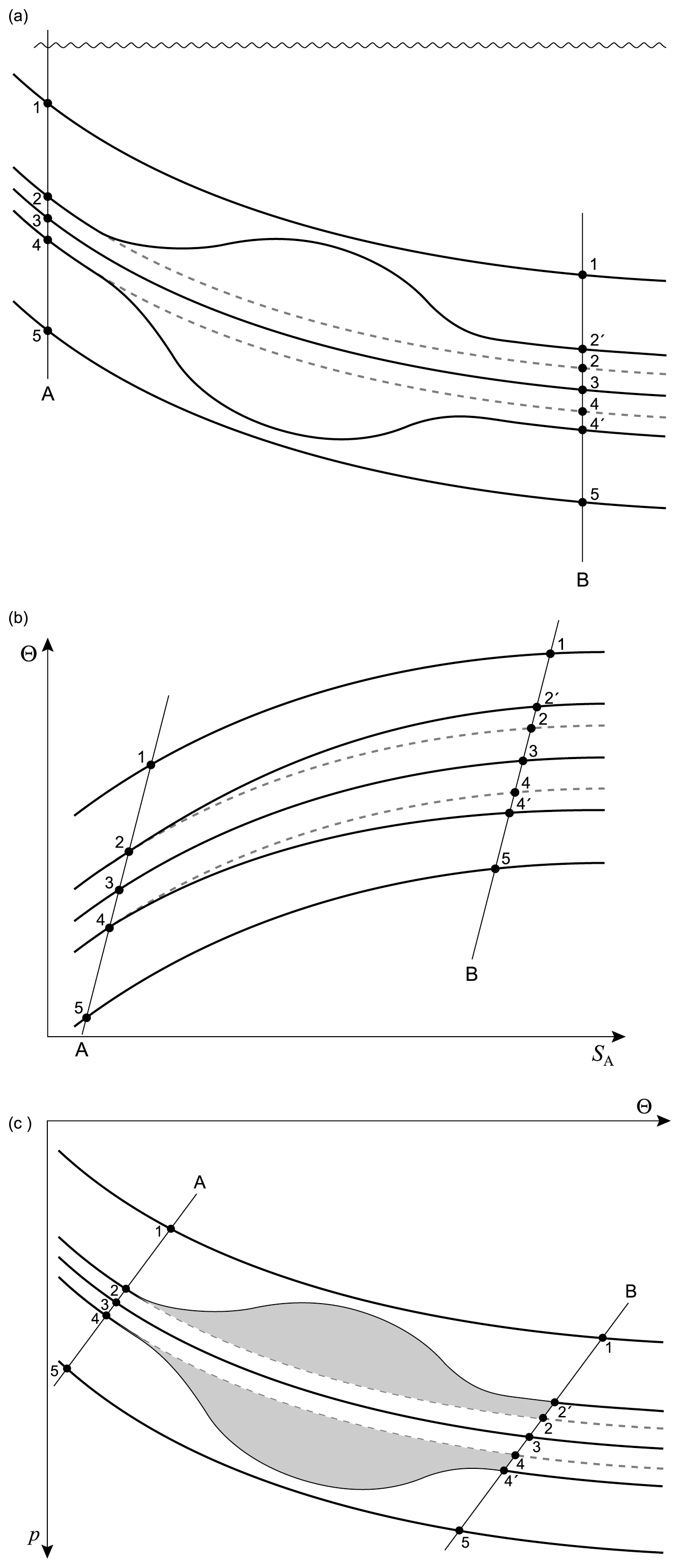
Figure 13 An ocean cross-section illustrating aspects of the epineutral variations of the integrating factor b.

13.4 Discussion of the expressions for the integrating factor

In the above we have found in the special case when ∇_nP=0, that ${\mathrm{\nabla }}_n\ln b=-\mathit{\rho }{g}^{\mathrm{2}}{N}^{-\mathrm{2}}{T}_{\mathrm{b}}{\mathrm{\nabla }}_n\mathrm{\Theta }$ and when ∇_nΘ=0, that ${\mathrm{\nabla }}_n\ln b=-g{N}^{-\mathrm{2}}({\mathit{\alpha }}_P{\mathrm{\Theta }}_z-{\mathit{\beta }}_P{S}_{{\mathrm{A}}_z}){\mathrm{\nabla }}_{n}P$, while in the general case we have found in Eq. (70) that ∇_nln b is the sum of these two contributions. It makes sense that the general case would be the sum of the two special cases since we expect the general expression for ∇_nln b to be linear in the two relevant epineutral gradients, ∇_nΘ and ∇_nP, consistent with the expansion of ∇_pκ in terms of ∇_nΘ and ∇_nP in going from Eq. (69) to Eq. (70). But the two special cases have delivered something that the general case has not, namely that in the two special cases we have been able to find expressions for the integrating factor b in terms of oceanographic properties on a single vertical water column rather than only in terms of its epineutral gradient through ∇_nln b; recall from Eqs. (60) and (65) that the integrating factor in the two special cases are $\stackrel{\mathrm{̃}}{b}[-g{N}^{-\mathrm{2}}(\ln \stackrel{\mathrm{̃}}{r}{)}_z]$ and $\stackrel{\mathrm{̃}}{b}[-g{N}^{-\mathrm{2}}(\ln {\stackrel{\mathrm{̃}}{\mathit{\rho }}}^{\mathrm{\Theta }}{)}_z]$, respectively. Given this knowledge we may be tempted to approximate the integrating factor in the general case as the product of these two expressions that apply in the special cases. That is, an approximation to the integrating factor might be thought to be

$$\begin{array}{}\text{(73)}& \begin{array}{rl}b& ={\displaystyle \frac{\text{NSPV}}{f{N}^{\mathrm{2}}}}={\displaystyle \frac{-g(\ln \mathit{\gamma }{)}_z}{N^{\mathrm{2}}}}\\ & \approx \stackrel{\mathrm{̃}}{b}\left[{\displaystyle \frac{-g(\ln \stackrel{\mathrm{̃}}{r}{)}_z}{N^{\mathrm{2}}}}\right]\left[{\displaystyle \frac{-g(\ln {\stackrel{\mathrm{̃}}{\mathit{\rho }}}^{\mathrm{\Theta }}{)}_z}{N^{\mathrm{2}}}}\right]\end{array}\end{array}$$

This equation is exact at finite amplitude in the two special cases ∇_nP=0 and ∇_nΘ=0, but Dr. Geoff Stanley (personal communication, 2025) has found that with a reference fluid parcel $({\stackrel{\mathrm{̃}}{S}}_{\mathrm{A}},\stackrel{\mathrm{̃}}{\mathrm{\Theta }},\stackrel{\mathrm{̃}}{P})$ near the equator on a given approximately neutral surface, this expression is not accurate in either the Southern Ocean or the North Atlantic. Hence, we are not justified in simply multiplying the two expressions for the integrating factor that apply in the two special case. That is, Eq. (73) is not a reasonable approximation to Eq. (71).

The rather simple-looking relationship (69), namely ${\mathrm{\nabla }}_n\ln b=\mathit{\rho }{g}^{\mathrm{2}}{N}^{-\mathrm{2}}{\mathrm{\nabla }}_p\mathit{\kappa }$, was published by McDougall (1988), and in the 38 years since 1988 I have sought a simple physical explanation of it, but without success. The progress reported here in understanding this relationship is limited to the realization that the terms in ∇_nΘ and ∇_nP that appear on the right-hand sides (Eq. 59) and (Eq. 64) of the two special cases are in fact the same terms in ∇_nΘ and ∇_nP whose sum is the right-hand side of the general expression (Eq. 70) for ∇_nln b. That is, we can claim to understand the general equation Eq. (71) for b in the two special cases, and in those two special cases, expressions have been found for the integrating factor that avoid the need to perform an epineutral integral. Given the almost four decades that have elapsed since McDougall (1988), I am quite disappointed not to have found a deeper understanding and faster progress on this topic!

14 Conclusions

This article reviews the aspects of physical oceanography in which thermodynamic concepts underlie modern oceanographic practice. These thermodynamic concepts are central to the research that led to TEOS-10 (the International Thermodynamic Equation Of Seawater – 2010) and also to the choices of variables that TEOS-10 recommended for oceanographic use. The Fundamental Thermodynamic Relationship and the First Law of Thermodynamics underlie all of seawater thermodynamics, and the derivations of these equations are outlined in Sect. 2 of this review.

Two important and commonly used quantities in physical oceanography and climate science are the ocean heat content (OHC) and the meridional heat transport of the ocean circulation. To evaluate the ocean heat content and the oceanic meridional transport of heat one would like to use a heat-like variable whose amount and whose transport can be compared to the air–sea flux of heat. An ideal variable for this purpose would be both a “potential” variable and a “conservative” variable, and these two attributes of thermodynamic variables are discussed in Sect. 3 above. We have discussed prior choices for evaluating the OHC and the meridional heat transport and have shown in Sect. 5 that the use of Conservative Temperature for these purposes is superior to using the previously suggested options; Conservative Temperature is a “potential” variable, and its non-conservation is just 1 % of that of potential temperature.

To be specific, the ocean heat content and the meridional heat flux should not be evaluated using either in-situ temperature or potential temperature, and these evaluations should not involve a spatially variable specific heat capacity. Rather, Conservative Temperature should be used along with the constant specific heat capacity, $c_p^{\mathrm{0}}\equiv$ 3991.86795711963 $\mathrm{J}{\mathrm{kg}}^{-\mathrm{1}}{\mathrm{K}}^{-\mathrm{1}}$. This recommendation applies to both observed ocean data and to the output of ocean models.

A new thermodynamic potential function has been introduced in Sect. 6 where it was shown that with Conservative Temperature as the temperature variable (as opposed to in-situ temperature or potential temperature), the thermodynamic information contained in enthalpy, $\widehat{h}(S_{\mathrm{A}},\mathrm{\Theta },P)$, is completely separate to the thermodynamic information contained in entropy, $\widehat{\mathit{\eta }}(S_{\mathrm{A}},\mathrm{\Theta })$. Such thermodynamic independence is not the case for the pair $h(S_{\mathrm{A}},T,P)$ and $\mathit{\eta }(S_{\mathrm{A}},T,P)$, nor for the pair $\stackrel{\mathrm{̃}}{h}(S_{\mathrm{A}},\mathit{\theta },P)$ and $\stackrel{\mathrm{̃}}{\mathit{\eta }}(S_{\mathrm{A}},\mathit{\theta })$. As a consequence, all of the following quantities, internal energy u, specific volume v, the thermal expansion coefficient α, the saline contraction coefficient β, the adiabatic compressibility κ, the speed of sound c, the adiabatic lapse rate of ln (T) (Eq. 16), and the ratio of the absolute in-situ and potential temperatures, $(T_{\mathrm{0}}+t)/(T_{\mathrm{0}}+\mathit{\theta })$, (Eq. 17), depend only on $\widehat{h}(S_{\mathrm{A}},\mathrm{\Theta },P)$ and are independent of $\widehat{\mathit{\eta }}(S_{\mathrm{A}},\mathrm{\Theta })$. This is a rather neat and appealing separation of the influence of enthalpy and entropy on these commonly used thermodynamic quantities. Since enthalpy is simply the following pressure integral of specific volume,

$$\begin{array}{}\text{(74)}& \widehat{h}(S_{\mathrm{A}},\mathrm{\Theta },P)=c_p^{\mathrm{0}}\mathrm{\Theta }+{\int }_{P_{\mathrm{0}}}^P\widehat{v}\left(S_{\mathrm{A}},\mathrm{\Theta },P^{\prime }\right)d{P}^{\prime },\end{array}$$

all of the above-listed thermodynamic quantities can be also found from knowledge of the Roquet et al. (2015) polynomial expression for specific volume, $\widehat{v}(S_{\mathrm{A}},\mathrm{\Theta },P)$, without needing any additional information about entropy.

TEOS-10 recognises that Practical Salinity, which depends on the electrical conductivity of seawater, is affected by the non-standard composition of seawater in a different way than is specific volume. This issue is addressed by TEOS-10 by defining the Absolute Salinity of seawater as the salinity that gives the correct specific volume (at the given temperature and pressure). Two different methods are summarised for relating the measured Practical Salinity to the Absolute Salinity that is needed to evaluate specific volume (and thereby, the thermal wind relationship).

Section 9 has shown that the temperature variable in ocean models must be interpreted as being Conservative Temperature because otherwise some of the heat that the atmosphere gives to (or receives from) the ocean disappears at the air–sea boundary in an unacceptable manner. Section 9 also makes clear that the salinity variable in both TEOS-10 and EOS-80 based ocean models should be interpreted as Preformed Salinity S_∗ (or $S_{\ast }/u_{\text{PS}}$ in the case of EOS-80 models).

It is shown in Sect. 9 that since ocean models to date have made no attempt to include the effects of the variable composition of seawater on the model's specific volume, meridional overturning transports can be in error by an estimated 13.5 % because of this neglect. Presumably the meridional heat transport in ocean models is also in error by a similar percentage, although this has not yet been studied. While this 13.5 % percentage figure is poorly known, and this percentage has only been estimated for the North Atlantic, it seems urgent to address this issue in ocean and climate models.

We have reviewed the thermodynamic reasoning that justifies the neutral tangent plane as being the local surface in which the strong lateral mixing of mesoscale turbulence occurs. The confusing subject of the path-dependent nature of neutral surfaces is also introduced, and some potential implications are discussed. This area of oceanographic research has attracted very little research and very few papers, but nevertheless there are several options for forming surfaces that are approximately neutral, and these options are discussed in Sect. 12.2. It is customary to take the planetary potential vorticity to be the Coriolis frequency multiplied by the square of the buoyancy frequency, but due to the thermobaric nonlinearity of the equation of state, this is not the case; Sect. 13 summarises what is known about this complication.

Looking forward, the most important improvement that is sorely needed in ocean models is to account for the difference between Absolute Salinity S_A and Preformed Salinity S_∗ (Preformed Salinity being the salinity variable of all ocean models to date). Because of the variable composition of seawater, approximately half of the locations deeper than 1000 m in ocean models have the thermal wind in error by more than 3 %. The suggested way of including this effect of biogeochemistry on specific volume in ocean models is discussed in Sects. 8 and 9 and involves the use of Eq. (37). An alternative method of allowing for the variations of seawater composition by relaxing towards existing observations has also been suggested by IOC et al. (2010), Wright et al. (2011), McDougall and Barker (2011) and McDougall et al. (2013).

Another refinement in ocean models that might be contemplated at some stage in the future is to include the dissipation of turbulent kinetic energy as a source of heat in the evolution equation of Conservative Temperature in ocean models. As discussed in Sects. 7 and 9 and in Fig. 7, this is a small positive definite source of heat, and when expressed as a surface flux of heat, only 5 % of the associated surface heat fluxes exceed the rather small surface heating of the ocean of 10 mW m⁻². Hence this refinement in the treatment of the First Law of Thermodynamics is trivial in comparison with the rather urgent need to include the effects of biogeochemistry (that is, $S_{\mathrm{A}}-S_{\ast }$) on specific volume and thereby on the ocean circulation and the meridional heat flux.