Response of a semi-enclosed sea to perturbed freshwater and open ocean salinity forcing

The sensitivity of Baltic Sea salinities to changed freshwater forcing and other forcing factors have been debated during the last decades, since changed salinities would have large impacts on the marine ecosystems, and since this parameter still shows a high degree of uncertainty in regional climate projections. In this study, we performed a sensitivity experiment where freshwater forcing and salinities at the outer boundaries of the North Sea were perturbed in a systematic way in order to obtain a second-order Taylor polynomial of the statistical steady state mean salinity. The polynomial was constructed based on perturbations of a 57 year long hindcast run for the period 1961–2017 with a regional ocean model covering the North Sea and the Baltic Sea. The results show that the Baltic Sea is highly sensitive to freshwater forcing, and that about one third of the boundary salinity change propagates into the Baltic Sea. The results are also analysed in terms of a total exchange flow analysis in the entrance region, and it is found that the Baltic Sea salinity sensitivity to freshwater forcing to a large degree can be explained by increased freshwater input causing (1) dilution inside the Baltic Sea, (2) decreased inflows caused by changes to the mean sea level gradient in the entrance region, and (3) reduced inflow salinities due to recirculation of outflowing Baltic Sea water in the entrance region where the inflow water consists of about two parts outflowing Baltic water and one part North Sea water. Besides providing new understanding of the processes that govern the Baltic Sea salinity sensitivity to freshwater forcing, the results of this study provide means of quickly assessing Baltic Sea salinity changes based on changes of North-East Atlantic salinities and Baltic Sea freshwater forcing.

1 Introduction

The Baltic Sea, Fig. 1, is a brackish, semi-enclosed sea in northern Europe, connected to the North Sea through a narrow and shallow entrance area. Marine ecosystems in the Baltic Sea have adjusted to the brackish (mostly less than 12 psu) conditions through thousands of years, and salinity changes are expected to have large impacts on ecosystems. For example, a cumulative impact study showed that a projected decrease in salinity together with increased temperatures and decreasing sea ice cover for the RCP4.5 and RCP8.5 scenarios are as important as the cumulative impacts of all other present anthropogenic pressures, e.g. fisheries, shipping, and eutrophication (Wåhlström et al., 2022). Projections of future salinities show a large spread with a range of about ±2 psu change by 2100 (e.g. Meier et al., 2021). Most regional ocean downscalings show a salinity decrease due to increased future precipitation, whereas some of those that also include sea level rise show increased salinities due to larger inflows of salt (e.g. Meier et al., 2017). In order to reduce the spread, there is a need of better understanding of the relative importance of various processes that influence the Baltic Sea salinity.

Figure 1 Model bathymetry for the North Sea/Baltic Sea region with red line indicating position of the Northern Kattegat transect and orange lines indicating the position of the sill transects. Yellow markers show the position of observation stations BY5 (circle), BY15 (triangle), and BY38 (star). Basin abbreviations are: Sk: Skagerrak, Kg: Kattegat, and GoB: Gulf of Bothnia. Note that the depth contours are non-linearly distributed.

Salinities in the Baltic Sea are the result of a balance between precipitation and evaporation over the Baltic Sea and its watershed, inflow of saline water through the entrance, and outflow of mixed water (e.g. Lehmann et al., 2022). This leads to a predominantly salinity stratified water body with a halocline at about 60–80 m depth in the Baltic proper, although seasonally a thermocline develops at 10–30 m depth over most parts of the Baltic Sea. Mean freshwater net input is about 15 000–16 000 m³ s⁻¹ (Meier et al., 2019). This consists of both river runoff and precipitation minus evaporation, with river runoff being the dominant component with a mean of about 14 000 m³ s⁻¹ and interdecadal variability of 1000–2000 m³ s⁻¹ (e.g. Meier et al., 2019). The inflow of saline water from the Kattegat is of about the same magnitude (Knudsen, 1900; Burchard et al., 2018). It is to a large degree barotropic, i.e. caused by wind-forced sea level differences between southern Kattegat and the south-western Baltic Sea, although there are also baroclinic inflows driven by the density difference between surface waters in Kattegat and the southern Baltic Sea (e.g. Mohrholz, 2018). Smaller barotropic inflows occur regularly, and mainly through the Sound, and do explain a large part of the salt import to the Baltic Sea. Larger inflows, so-called Major Baltic Inflows (MBIs) that are dense enough to modify the Baltic deepwater, flow through both the Sound and the Belts, and do occur much less frequently and mainly during winter time (Mohrholz, 2018).

Analysis of historical records and model results indicate a large sensitivity of Baltic Sea salinities to freshwater input. Rodhe and Winsor (2003) propose a more than 3 % salinity decrease for a 1 % freshwater increase based on observational data. Modeling studies show somewhat smaller sensitivities, 1 %–1.5 % salinity decrease for a 1 % freshwater increase (Stigebrandt and Gustafsson, 2003; Meier and Kauker, 2003).

Based on a long hindcast simulation, Radtke et al. (2020) claim that multidecadal surface salinity variability in the Baltic Sea is mainly caused by modulated precipitation over the watershed, with about 27 % being caused by direct dilution of the Baltic Sea and the rest being caused by reduced inflows of salt. Meier et al. (2023) find that the salinity response to freshwater forcing is dominated by direct dilution and reduced inflow salinities due to increased freshwater volumes in Kattegat, whereas the model study of Stigebrandt and Gustafsson (2003) include both decreased inflow volumes and decreased salinities in Kattegat as explanations for the Baltic Sea salinity response to freshwater forcing.

Other factors that influence Baltic Sea salinities are zonal winds and atmospheric pressure gradients in the entrance area, through their influence on MBIs, e.g. Schimanke and Meier (2016), and sea level rise (e.g. Hordoir et al., 2015). Another potentially important factor for Baltic Sea salinities is changing salinities in the North-East Atlantic. This factor has not been investigated thoroughly earlier since most regional ocean models used for Baltic Sea projections have had an outer boundary in northern Kattegat or eastern Skagerrak where the salinities may be influenced by salinity changes within the domain. Global climate model simulations indicate that salinity in the North-East Atlantic is likely to change in response to increased freshwater input from melting ice masses, an intensified hydrological cycle, and weakening of the Atlantic Meridional Overturning Circulation (AMOC), with a substantial inter-model spread in projected salinity changes by 2100 (Molodtsov et al., 2025). This will in turn cause changes in boundary conditions for a regional downscaling of the North Sea and the Baltic Sea when these global climate models are used. There is therefore a need to quantify the importance of North-East Atlantic salinities on the Baltic Sea salinities.

In this study we focus on the steady state sensitivity of Baltic Sea salinities to (i) net freshwater input to the Baltic Sea, and to (ii) changing salinities at the boundary of the North Sea, since we know that freshwater input is important, and because we want to know how important the boundary salinities are relative to that. We use a 3D model setup of the Baltic Sea and the North Sea, where the open boundaries are influenced less by the Baltic Sea than most other earlier models used for Baltic Sea studies. We design the sensitivity experiment in order to estimate a second order Taylor polynomial based on the two variables freshwater input and boundary salinity, which can be used for interpolation and to some degree extrapolation of the Baltic Sea salinity changes based on changes of the two input variables. We also use total exchange flow analysis (e.g. Burchard et al., 2018) at two transects in the entrance region to quantify the physical processes that cause the sensitivity, including the influence of recirculation in the Kattegat and Belt Sea region. This turns out to result in new understanding and a simplified framework for estimating Baltic Sea salinities.

2 Methods

2.1 Experimental design: Taylor expansion

As mentioned in the introduction we are interested in the response of the Baltic Sea salinity to perturbations in precipitation/runoff and boundary salinity. Moreover, in this section we restrict our attention to study this response in a statistical steady state.

Let $\stackrel{\mathrm{‾}}{S}$ denote a long-time averaged salinity property, for example the basin mean salinity, defined through

$$\begin{array}{}\text{(1)}& \stackrel{\mathrm{‾}}{S}={\displaystyle \frac{\mathrm{1}}{V(t_{\mathrm{2}}-t_{\mathrm{1}})}}{\int }_{t_{\mathrm{1}}}^{t_{\mathrm{2}}}\mathrm{d}t{\int }_{V}s\mathrm{d}V,\end{array}$$

where V is the volume of the basin, t₁ and t₂ the start and end times of the averaging period and s the salinity. To study the response of $\stackrel{\mathrm{‾}}{S}$ to the aforementioned perturbations we approximate $\stackrel{\mathrm{‾}}{S}$ using a second order Taylor polynomial

$$\begin{array}{}\text{(2)}& \begin{array}{rl}\stackrel{\mathrm{‾}}{S}& \approx \stackrel{\mathrm{‾}}{S}({\text{SB}}_{\mathrm{0}},{\text{RP}}_{\mathrm{0}})+{\displaystyle \frac{\partial \stackrel{\mathrm{‾}}{S}}{\partial \text{SB}}}(\text{SB}-{\text{SB}}_{\mathrm{0}})+{\displaystyle \frac{\partial \stackrel{\mathrm{‾}}{S}}{\partial \text{RP}}}(\text{RP}-{\text{RP}}_{\mathrm{0}})\\ & +{\displaystyle \frac{\mathrm{1}}{\mathrm{2}}}{\displaystyle \frac{{\partial }^{\mathrm{2}}\stackrel{\mathrm{‾}}{S}}{\partial {\text{SB}}^{\mathrm{2}}}}(\text{SB}-{\text{SB}}_{\mathrm{0}}{)}^{\mathrm{2}}+{\displaystyle \frac{\mathrm{1}}{\mathrm{2}}}{\displaystyle \frac{{\partial }^{\mathrm{2}}\stackrel{\mathrm{‾}}{S}}{\partial {\text{RP}}^{\mathrm{2}}}}(\text{RP}-{\text{RP}}_{\mathrm{0}}{)}^{\mathrm{2}}\\ & +{\displaystyle \frac{{\partial }^{\mathrm{2}}\stackrel{\mathrm{‾}}{S}}{\partial \text{SB}\partial \text{RP}}}(\text{SB}-{\text{SB}}_{\mathrm{0}})(\text{RP}-{\text{RP}}_{\mathrm{0}}),\end{array}\end{array}$$

where SB and RP denote the boundary salinity and runoff+precipitation respectively, and the 0 subscript denotes the unperturbed state (i.e. long-time averages from a historical simulation). RP is normalized with the runoff + precipitation of the unperturbed state.

The choice of a second order Taylor polynomial as opposed to a simpler first order one is motivated by the fact that it gives us a chance to quantify the interaction between the two forcing terms through the cross-derivative term. To compute the coefficients for the Taylor polynomial, six runs are needed in addition to the unperturbed hindcast giving the $\stackrel{\mathrm{‾}}{S}({\text{SB}}_{\mathrm{0}},{\text{RP}}_{\mathrm{0}})$ term. The scheme is as follows:

$$\begin{array}{}\text{(3)}& {\displaystyle \frac{\partial \stackrel{\mathrm{‾}}{S}}{\partial \text{SB}}}=\left(\mathrm{2}h{)}^{-\mathrm{1}}\right(\stackrel{\mathrm{‾}}{S}({\text{SB}}_{\mathrm{0}}+h,{\text{RP}}_{\mathrm{0}})-\stackrel{\mathrm{‾}}{S}({\text{SB}}_{\mathrm{0}}-h,{\text{RP}}_{\mathrm{0}})),\text{(4)}& {\displaystyle \frac{\partial \stackrel{\mathrm{‾}}{S}}{\partial \text{RP}}}=\left(\mathrm{2}k{)}^{-\mathrm{1}}\right(\stackrel{\mathrm{‾}}{S}({\text{SB}}_{\mathrm{0}},{\text{RP}}_{\mathrm{0}}+k)-\stackrel{\mathrm{‾}}{S}({\text{SB}}_{\mathrm{0}},{\text{RP}}_{\mathrm{0}}-k)),\text{(5)}& {\displaystyle }\begin{array}{rl}{\displaystyle \frac{{\partial }^{\mathrm{2}}\stackrel{\mathrm{‾}}{S}}{\partial {\text{SB}}^{\mathrm{2}}}}& =h^{-\mathrm{2}}\left(\stackrel{\mathrm{‾}}{S}\right({\text{SB}}_{\mathrm{0}}+h,{\text{RP}}_{\mathrm{0}})-\mathrm{2}\stackrel{\mathrm{‾}}{S}({\text{SB}}_{\mathrm{0}},{\text{RP}}_{\mathrm{0}})\\ & +\stackrel{\mathrm{‾}}{S}({\text{SB}}_{\mathrm{0}}-h,{\text{RP}}_{\mathrm{0}})),\end{array}\text{(6)}& {\displaystyle }\begin{array}{rl}{\displaystyle \frac{{\partial }^{\mathrm{2}}\stackrel{\mathrm{‾}}{S}}{\partial {\text{RP}}^{\mathrm{2}}}}& =k^{-\mathrm{2}}\left(\stackrel{\mathrm{‾}}{S}\right({\text{SB}}_{\mathrm{0}},{\text{RP}}_{\mathrm{0}}+k)-\mathrm{2}\stackrel{\mathrm{‾}}{S}({\text{SB}}_{\mathrm{0}},{\text{RP}}_{\mathrm{0}})\\ & +\stackrel{\mathrm{‾}}{S}({\text{SB}}_{\mathrm{0}},{\text{RP}}_{\mathrm{0}}-k)),\end{array}\text{(7)}& {\displaystyle }\begin{array}{rl}{\displaystyle \frac{{\partial }^{\mathrm{2}}\stackrel{\mathrm{‾}}{S}}{\partial \text{SBdRP}}}& =\left(\mathrm{2}hk{)}^{-\mathrm{1}}\right(\stackrel{\mathrm{‾}}{S}({\text{SB}}_{\mathrm{0}}+h,{\text{RP}}_{\mathrm{0}}+k)-\stackrel{\mathrm{‾}}{S}({\text{SB}}_{\mathrm{0}}+h,{\text{RP}}_{\mathrm{0}})\\ & -\stackrel{\mathrm{‾}}{S}({\text{SB}}_{\mathrm{0}},{\text{RP}}_{\mathrm{0}}+k)+\mathrm{2}\stackrel{\mathrm{‾}}{S}({\text{SB}}_{\mathrm{0}},{\text{RP}}_{\mathrm{0}})\\ & -\stackrel{\mathrm{‾}}{S}({\text{SB}}_{\mathrm{0}}-h,{\text{RP}}_{\mathrm{0}})-\stackrel{\mathrm{‾}}{S}({\text{SB}}_{\mathrm{0}},{\text{RP}}_{\mathrm{0}}-k)\\ & +\stackrel{\mathrm{‾}}{S}({\text{SB}}_{\mathrm{0}}-h,{\text{RP}}_{\mathrm{0}}-k)),\end{array}\end{array}$$

where h is a salinity perturbation on the outer boundary, and k is a fractional perturbation of the precipitation and runoff. This means that in addition to the reference case $\stackrel{\mathrm{‾}}{S}({\text{SB}}_{\mathrm{0}},{\text{RP}}_{\mathrm{0}})$, the following integrations are needed: $\stackrel{\mathrm{‾}}{S}({\text{SB}}_{\mathrm{0}}+h,{\text{RP}}_{\mathrm{0}})$, $\stackrel{\mathrm{‾}}{S}({\text{SB}}_{\mathrm{0}}-h,{\text{RP}}_{\mathrm{0}})$, $\stackrel{\mathrm{‾}}{S}({\text{SB}}_{\mathrm{0}},{\text{RP}}_{\mathrm{0}}+k)$, $\stackrel{\mathrm{‾}}{S}({\text{SB}}_{\mathrm{0}},{\text{RP}}_{\mathrm{0}}-k)$, $\stackrel{\mathrm{‾}}{S}({\text{SB}}_{\mathrm{0}}+h,{\text{RP}}_{\mathrm{0}}+k)$ and $\stackrel{\mathrm{‾}}{S}({\text{SB}}_{\mathrm{0}}-h,{\text{RP}}_{\mathrm{0}}-k)$.

Note that a relative change in precipitation and runoff is not the same as a relative change in net freshwater input to a system, Q_f, since a large fraction of the precipitation is lost to evaporation, making $Q_{\mathrm{f}}/Q_{\text{f0}}$ smaller than RP. Evaporation is relatively constant between the different runs in this experiment, so the change in net freshwater input is about equal to the change in precipitation and runoff, but since Q_f is smaller than precipitation + runoff, the relative change in Q_f is about 28 % when the change in RP is 20 %.

2.2 Total exchange flow analysis

Analysing transports through a transect in salinity coordinates rather than Eulerian vertical coordinates (e.g. Walin, 1977; MacCready, 2011; Burchard et al., 2018) enables quantification of water mass transformation and estuarine water exchange in a way very similar to the ideas behind the Knudsen theorem (Knudsen, 1900). The time averaged advective inflows of volume and salt mass in water with salinity larger than s can be written as

$$\begin{array}{}\text{(8)}& Q\left(s\right)=\stackrel{\mathrm{‾}}{{\int }_{A\left(s\right)}u\mathrm{d}A},\end{array}$$

and

$$\begin{array}{}\text{(9)}& F\left(s\right)=\stackrel{\mathrm{‾}}{{\int }_{A\left(s\right)}su\mathrm{d}A},\end{array}$$

where A(s) at any time is the transect area with salinity larger than s, u is the horizontal velocity component normal to the transect pointing into the estuary, and overbar denotes time averaging. These can be integrated into in- and outflows through

$$\begin{array}{}\text{(10)}& {\displaystyle }{Q}_{\text{in}}={\int }_{\mathrm{0}}^{\mathrm{\infty }}max\left(\mathrm{0},-{\displaystyle \frac{\partial Q}{\partial s}}\right)\mathrm{d}s,\text{(11)}& {\displaystyle }{Q}_{\text{out}}={\int }_{\mathrm{0}}^{\mathrm{\infty }}max\left(\mathrm{0},{\displaystyle \frac{\partial Q}{\partial s}}\right)\mathrm{d}s,\text{(12)}& {\displaystyle }{F}_{\text{in}}={\int }_{\mathrm{0}}^{\mathrm{\infty }}max\left(\mathrm{0},-{\displaystyle \frac{\partial F}{\partial s}}\right)\mathrm{d}s,\text{(13)}& {\displaystyle }{F}_{\text{out}}={\int }_{\mathrm{0}}^{\mathrm{\infty }}max\left(\mathrm{0},{\displaystyle \frac{\partial F}{\partial s}}\right)\mathrm{d}s,\end{array}$$

where

$$\begin{array}{}\text{(14)}& max(x,y)=\left\{\begin{array}{ll}x,& x\ge y\\ y,& x<y\end{array}\right..\end{array}$$

Now, mean inflow and outflow salinities can be calculated as

$$\begin{array}{}\text{(15)}& S_{\text{in}}={\displaystyle \frac{F_{\text{in}}}{Q_{\text{in}}}},S_{\text{out}}={\displaystyle \frac{F_{\text{out}}}{Q_{\text{out}}}}.\end{array}$$

When averaged over long time relative to the residence times of salt and freshwater in the system, and changes to inflow and freshwater input, the accumulation of volume and salt are small relative to the in- and outflow transports, and a steady state volume and salt budget analysis results in the Knudsen relations (see Burchard et al., 2018, for a discussion)

$$\begin{array}{}\text{(16)}& {\displaystyle }{Q}_{\text{in}}={\displaystyle \frac{S_{\text{out}}}{S_{\text{in}}-S_{\text{out}}}}{Q}_{\mathrm{f}},\text{(17)}& {\displaystyle }{Q}_{\text{out}}={\displaystyle \frac{S_{\text{in}}}{S_{\text{in}}-S_{\text{out}}}}{Q}_{\mathrm{f}},\end{array}$$

where Q_f is the mean integrated freshwater input (runoff + precipitation − evaporation) to the estuary inside the investigated transect.

For two transects, A and B, where B is located closest to the open ocean, part of the outflow through section A, Q_RA, is recirculated and contribute to the inflow through section A, while the rest, Q_outA−Q_RA, flows out through section B. Similarly, part of the inflow through section B, Q_RB, is recirculated and contribute to the outflow through section B, while the rest, Q_inB−Q_RB, contributes to the inflow though section A. The corresponding salt and volume inflows through section A can be written as

$$\begin{array}{}\text{(18)}& {\displaystyle }{Q}_{\text{inA}}{S}_{\text{inA}}=(Q_{\text{inB}}-Q_{\text{RB}})S_{\text{inB}}+Q_{\text{RA}}{S}_{\text{outA}},\text{(19)}& {\displaystyle }{Q}_{\text{inA}}=Q_{\text{inB}}-Q_{\text{RB}}+Q_{\text{RA}}+\mathit{\gamma }\mathrm{\Delta }{Q}_{\mathrm{f}},\end{array}$$

where ΔQ_f is the freshwater input between section A and B and γ is the fraction of this that enters the Baltic Sea. The recirculation fluxes can now be found as

$$\begin{array}{}\text{(20)}& {\displaystyle }{Q}_{\text{RA}}={\displaystyle \frac{Q_{\text{inA}}(S_{\text{inB}}-S_{\text{inA}})-\mathit{\gamma }\mathrm{\Delta }{Q}_{\mathrm{f}}{S}_{\text{inB}}}{S_{\text{inB}}-S_{\text{outA}}}},\text{(21)}& {\displaystyle }{Q}_{\text{RB}}={\displaystyle \frac{Q_{\text{outB}}(S_{\text{outB}}-S_{\text{outA}})+(\mathrm{1}-\mathit{\gamma })\mathrm{\Delta }{Q}_{\mathrm{f}}{S}_{\text{outA}}}{S_{\text{inB}}-S_{\text{outA}}}}.\end{array}$$

These expressions are similar to the efflux/reflux expressions first presented by Cokelet and Stewart (1985), except for the addition of local runoff. They basically express that the water masses flowing out from the region bounded by the A and B sections are a result of turbulent mixing between the water masses flowing into the region. In- and outflows, and recirculation fluxes, were calculated as described above for two transects, Fig. 1, one in northern Kattegat (section B), and one that includes the Darss- and Drogden sills at the rim of the Baltic Sea (section A). The recirculation fluxes are therefore caused by water mass modifications in Kattegat or in the Belts and the Sound. Temporal averages were based on the period 1990–2017.

2.3 Model setup

Our experiments use a NEMO 4.2 configuration of the North Sea and Baltic Sea region (see Fig. 1). The configuration builds on a previous NEMO 3.6 configuration with evaluations of ocean and sea-ice parameters presented in Hordoir et al. (2019) and Pemberton et al. (2017), respectively. The horizontal resolution is 0.055° in the zonal and 0.033° in the meridional direction, which amounts to a nominal resolution of 3.7 km (2 nmi). To adapt the configuration to NEMO 4.2 we have changed the tracer advection scheme to 4th order Flux Corrected Transport (FCT) scheme, and the lateral viscosity formulation from a laplacian to a bi-laplacian operator. To improve the salinity dynamics of the model configuration we have changed the vertical coordinate system from the geopotential Z-partial steps formulation (used in Hordoir et al., 2019) to the terrain-following Multi-Envelope s-coordinate (MEs) system developed by Bruciaferri et al. (2018). The MEs coordinates are configured to use 2 envelopes. The upper envelope ranges between the surface and 250 m and uses 43 levels, and the lower envelope covers all depths below 250 m using 13 levels. We thus retain the 56 vertical levels used in Hordoir et al. (2019) but gain a higher vertical resolution in the Baltic Sea. In a separate study (Pemberton et al., 2026) we make a thorough evaluation of the impact of the vertical coordinate system on the Baltic Sea hydrography and circulation. Here we instead restrict our evaluation to compare the mean vertical salinity distribution and surface/bottom salinity evolution for the hindcast run to observations at three stations.

Figure 2 Salinity profiles at three selected stations in the Baltic Sea for the period 1970 to 2017. The blue solid lines represent the temporal mean of the hindcast experiment, and the dashed lines the 5th and 95th percentiles. The grey dots represent observed salinity from the SHARK database.

The hindcast run is the reference simulation for the perturbation runs described in Sect. 2.4. It is a run from 1961 to 2017 based on the best available forcing. Before performing the hindcast and perturbation runs, we spun up the model circulation by using initial conditions for salinity and temperature from the Janssen et al. (1999) climatology, with ocean currents and sea surface height set to zero. Then we ran the model three cycles repeating the same 10 years period using atmospheric, runoff and open boundary forcing from 1961–1970 so that model dynamics reached near-equlibrium level. The meteorological forcing was derived from the UERRA regional reanalysis (Dahlgren et al., 2016), which offers a spatial resolution of 11 km and a temporal resolution of 1 h for parameters such as wind, air pressure, air temperature, humidity, and both solar and long-wave downward radiation. Precipitation (rain and snow) is provided at a temporal resolution of 12 h. River runoff forcing was provided as daily values from a dedicated simulation with the Hydrological Predictions for the Environment model with the European application v.3.1.8 (E-HYPE; Donnelly et al., 2016). The open boundary forcing includes barotropic currents, sea level, nine tidal constituents, and monthly salinity and temperature data. The barotropic currents and sea level were calculated using the 2D North Atlantic Model (NOAMOD; She et al., 2007) storm-surge model. These values were adjusted for baroclinic influences by incorporating monthly sea level data from the European Centre for Medium-Range Weather Forecasts' Ocean Reanalysis System 4 (ORAS4), which enhances the description of the North Sea ocean circulation. The salinity and temperature profiles are monthly mean values interpolated from the ORAS4 configuration (Balmaseda et al., 2013).

To illustrate the model performance, observations were taken from the Swedish archive for oceanographic data (SHARK, https://www.smhi.se, last access: 12 January 2026), at three selected stations in the Baltic Sea, located at different distances from the entrance (see Fig. 1). Vertical salinity profiles from the three stations (Fig. 2) show that the salinity stratification and the range of variability are well described by the model at the three stations. The temporal variability in the surface water and in the bottom water (Fig. 3) show that surface water salinity is well represented by the model both with respect to short-term variability and long-term trends. Note that since the observational stations are often located near the deepest point in a basin, the bottom water comparison was done somewhat above the bottom to make the time series representative for the water volume below the halocline rather than for just a small local bottom water volume. Both model and observations show a decrease in surface water salinity between 1980 and 2000. Before 1980 the model surface salinities are slightly larger than the observed salinities, which may be due to an adjustment from too high initial salinities. Near-bottom water model salinities also show similar temporal variability as in observations with a long period between 1980 and 1993 without strong inflows of saline water. Generally, the model salinities compare as well with observations as those of the better models in the Baltic Sea Model Intercomparison Project (Gröger et al., 2022) and the model is therefore well suited for the sensitivity study which is the focus of this work.

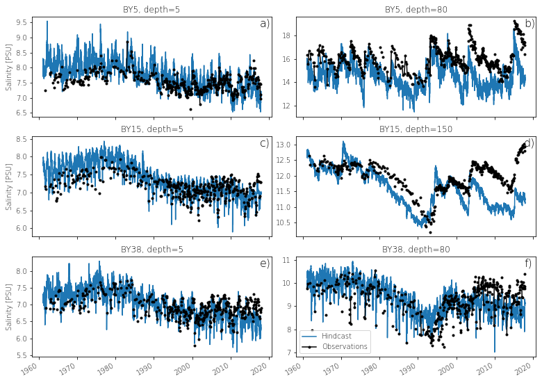
Figure 3 Time-evolution of surface water (left column) salinity and bottom water (right column) salinity at three selected stations in the Baltic Sea. The blue solid lines are from the hindcast experiment and the black dots observations from the SHARK database. The approximate station depths are BY5: 90 m, BY15: 240 m, BY38: 100 m.

2.4 Model runs

To investigate the salinity dynamics of the Baltic Sea in response to variations in freshwater input and boundary salinity using a Taylor expansion approach (Sect. 2.1), we performed a series of model simulations in which these two factors were systematically perturbed over the period from 1961 to 2017, see Table 1. In these runs, either boundary salinities were maintained the same as in the reference run while freshwater input was varied by ±20 % relative to the reference scenario (runs RP+ and RP-), or boundary salinities (meaning the salinities at the open boundaries in the Channel and between the Orkney Islands and Norway, Fig. 1) were altered by ±0.5 psu compared to the reference experiment while runoff and precipitation was maintained equal to those of the reference run (runs SB+ and SB-). These choices for size of perturbations were somewhat arbitrarily chosen to yield a span containing the long-term variability and expected effects of climate change. For river runoff, 20 % is in the upper end of the expected increase in runoff by 2100 (e.g. Saraiva et al., 2019). For boundary salinity 0.5 psu represents rather well the expected variability in changes at the outer boundaries of the North Sea (e.g. Quante and Colijn, 2016). However, the variability in projected salinity changes between different GCMs is rather in the range of 1–2 psu, so in hindsight we could have chosen a larger perturbation value.

Table 1 Model runs performed.

The fractional changes in freshwater input were applied using NEMO namelist options for runoff and precipitation multipliers. To capture interaction terms, two experiments were performed (RP+SB+ and RP-SB-). Finally, three additional runs were carried out to evaluate the polynomial's validity outside the bounds of the runs used to determine the polynomial. These involved; a 50 % increase in freshwater input and a 1.0 psu rise in boundary salinity from the reference run (RP++SB++), a 10 % increase in freshwater input and 0.6 psu rise (RP+10SB+06) and 0.6 psu decrease (RP+10SB-06) in boundary salinity.

3 Results

3.1 Temporal and spatial salinity changes

The time series of yearly mean salinities averaged over the whole Baltic Sea volume inside the sill transect (Fig. 1) are shown in Fig. 4. It is clearly seen that the salinities show a large sensitivity towards freshwater forcing, with a difference from the hindcast run of about 2 psu. When freshwater forcing increases (red lines), the salinities decrease relative to the hindcast (black solid line), and when the freshwater forcing decreases (blue lines), the salinities increase. The green lines are the additional runs (runs 7–9 in Table 1) and the solid green line corresponds to the most extreme case with 50 % increase in runoff and precipitation. The changes caused by changing boundary salinity (dashed and dotted lines) are much smaller, maybe due to the choice of perturbation values. The adjustment to new forcing is seen to be largest during the first 20–30 years and then level out relative to the hindcast run. In the following, the period 1990–2017 is therefore chosen to represent the “steady state” conditions where the runs have adjusted to the changed forcing.

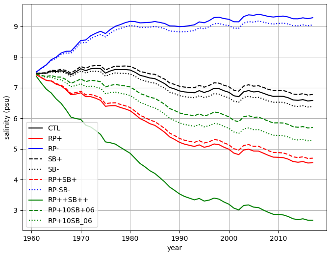
Figure 4 Yearly mean salinities for the Baltic Sea averaged over the volume inside the sill transect.

Figure 5 shows maps of depth averaged salinity changes relative to the hindcast (CTL) run, averaged over the period 1990–2017. For the precipitation and evaporation change (RP+ and RP-) runs, the salinity changes are larger inside the Baltic Sea than outside and rather homogeneous, however gradually somewhat decreasing as we move north. The changes for these runs are almost equal but of opposite sign, except for the Gulf of Bothnia where the salinity decrease is smaller for increasing runoff than the salinity increase for decreasing runoff. In Kattegat, changes are mainly seen in the shallow areas towards the Danish coast and close to the Swedish coast, and in Skagerrak and the North Sea, changes are mainly concentrated in the coastal areas.

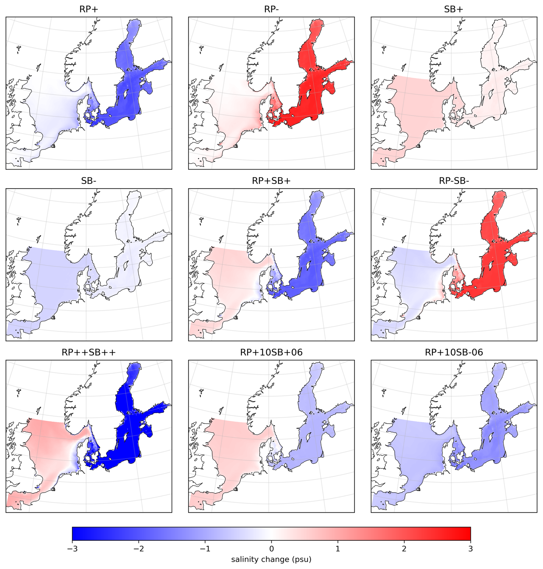
Figure 5 Changes relative to hindcast (CTL) run for depth averaged mean salinities for the period 1990–2017.

The boundary salinity changes (SB+ and SB-) manifest themselves rather uniformly in the North Sea, Skagerrak and Kattegat. Inside the Baltic Sea, the changes are much smaller but still distributed rather uniformly.

For combinations of the perturbations, the changes caused by runoff and precipitation dominate in the Baltic Sea, Kattegat and along the coasts of Skagerrak and the North Sea, while the boundary salinity changes dominate in the open parts of the North Sea and Skagerrak.

3.2 Taylor expansion

Figure 6, shows the second order Taylor polynomial for $\stackrel{\mathrm{‾}}{S}$. The coefficients of the polynomial are given in Table 2. It is quite clear from the figure that the response to perturbations is close to linear in h (boundary salinity change), and nonlinear in k (runoff and freshwater input change). The latter is seen through the increasing distance between level curves as k increases. The interaction term, the cross derivative, is not very important. It is negative (Table 2), meaning that for positive changes in RP and SB, the salinity decrease will be slightly larger with than without the interaction term. The change is, however, small, which can easiest be seen by comparing polynomial plots with and without (not shown) the interaction term. These two plots are very similar. It is also clear from Fig. 4 that boundary salinity changes are damped in the basin. The first derivative of $\stackrel{\mathrm{‾}}{S}$ with respect to SB is 0.36, indicating that a salinity change of 1 psu at the boundary gives a change in $\stackrel{\mathrm{‾}}{S}$ of 0.36 psu in the Baltic Sea.

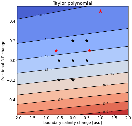
Figure 6 Taylor polynomial (psu) for $\stackrel{\mathrm{‾}}{S}$ as function of the change in salinity at the open boundaries (SB), and fractional change in precipitation and runoff (RP).

Table 2 Polynomial coefficients for second order polynomial of Baltic Sea mean salinities for the period 1990–2017.

The interpolation and extrapolation qualities of the polynomial are shown in Fig. 7. The scatter plot shows modeled $\stackrel{\mathrm{‾}}{S}$ against $\stackrel{\mathrm{‾}}{S}$ derived from the Taylor polynomial. The point with the largest deviation is from to the $\stackrel{\mathrm{‾}}{S}({\text{SB}}_{\mathrm{0}}+\mathrm{2}h,{\text{RP}}_{\mathrm{0}}+\mathrm{2.5}k)$ run (RP++SB++) which is a large extrapolation. Even so the quality is rather good. Note also that only the point $\stackrel{\mathrm{‾}}{S}({\text{SB}}_{\mathrm{0}},{\text{RP}}_{\mathrm{0}})$ is exactly equal for the polynomial and the model, but almost all the other points also fall on a near perfect line, indicating very good interpolation properties. Looking beyond $\stackrel{\mathrm{‾}}{S}$ one can also estimate Taylor polynomials for other quantities based on the present experiment, for example surface salinities, bottom salinities, or higher percentiles of the Baltic Sea salinity distribution. As an example, the Taylor polynomial for the 95th percentile of the Baltic Sea spatial salinity distribution gives a larger response to boundary salinity change than the mean salinity, with first derivative of the 95 % percentile with respect to SB being 0.57 where it is 0.36 for $\stackrel{\mathrm{‾}}{S}$. However, qualitatively, polynomials for different percentiles are relatively similar.

Figure 7 Comparison of modeled and Taylor polynomial $\stackrel{\mathrm{‾}}{S}$ at known points. Black stars are for runs used to calculate the polynomial and red stars are for the remaining runs. The lowest salinity comes from the $\stackrel{\mathrm{‾}}{S}(\text{SB}+\mathrm{2}h,\text{RP}+\mathrm{2}k)$ run and is thus a rather large extrapolation. The black straight line shows the 1:1 relationship.

3.3 Total exchange flow analysis

The inflow functions, Q and F, for volume and salt, defined in Eqs. (8) and (9), and averaged over the period 1990 to 2017, are shown in Figs. 8 and 9.

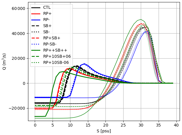
Figure 8 Cumulated inflows of volume, Q, of water with salinity larger than s as defined in Eq. (8), and for the period 1990–2017. Thick lines are for transports through the sill transect, and thin lines are for transports through the northern Kattegat transect. Inflows happen at salinity intervals with negative gradient of Q, whereas outflows happen at salinity intervals with positive gradient.

Figure 9 Cumulated inflows of salt, F, in water with salinity larger than s as defined in Eq. (9), and for the period 1990–2017. Thick lines are for transports through the sill transect, and thin lines are for transports through the northern Kattegat transect. Inflows happen at salinity intervals with negative gradient of F, whereas outflows happen at salinity intervals with positive gradient.

For the hindcast run, the net outflow, seen as Q at s=0, Fig. 8, is 15 700 m³ s⁻¹ at the sill transect and 16 400 m³ s⁻¹ at the northern Kattegat transect. The main outflows at the sill transect, seen as the part of Q with positive gradient with respect to salinity, have salinities between 7 and 11 psu, and the main inflows have salinities between 11 and 28 psu. At the northern Kattegat transect, the main outflows have salinities between 15 and 31 psu while the inflows happen at 31–36 psu. The strength of the inflow, seen as the maximum value of Q, is about 13 500 m³ s⁻¹ at the sill transect and 45 000 m³ s⁻¹ at northern Kattegat.

For increased runoff and precipitation, RP+, RP+SB+, and RP++SB++, the inflow strengths through the sill transect are reduced and the salinities of inflows and outflows are also decreased. For the northern Kattegat transect, the inflow strength increases for these cases, the outflow salinities decrease, whereas the inflow salinities are less affected.

The salinity and inflow strength changes for cases with decreasing runoff and precipitation are opposite to those for the cases with increasing runoff and precipitation.

Changing boundary salinities are mainly affecting the salinities of inflows and outflows at the northern Kattegat boundary, but do cause less changes to the inflows and outflows at the sill transect, and only small changes to the inflow and outflow strengths.

Figure 9 clearly illustrates that the overturning of salt in Kattegat and the Belts and Sound is much larger than within the Baltic Sea. Otherwise, it shows many of the same features as seen in Fig. 8. In a steady state condition, the net cumulated inflow of salt at small salinities should be zero. It is, however, seen that many of the curves have a small negative value there, i.e. a net outflow of salt, which corresponds to the negative mean salinity trend in the period 1990–2017 seen in Fig. 2.

The in- and out fluxes through the transects and the recirculation calculated from Eqs. (20) and (21) are shown for the hindcast run in Fig. 10. The recirculation fluxes are calculated using γ=0, i.e. assuming the local freshwater input between transects A and B is being added to the outflow through transect B. It is seen that the inflowing water to the Baltic Sea through transect A consists of about 64 % outflowing Baltic Sea water and 36 % inflowing Skagerrak water, and that the outflow through transect B consists of about 64 % inflowing Skagerrak water, 1 % local freshwater and 35 % outflowing Baltic Sea water.

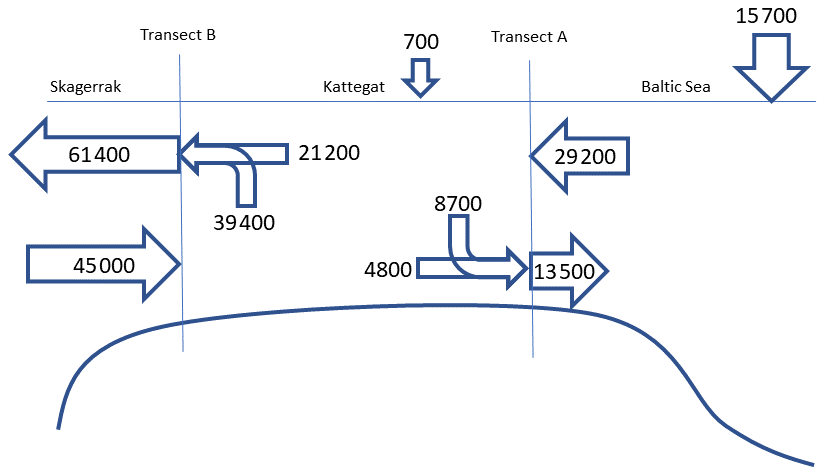
Figure 10 Mean volume fluxes for the period 1990–2017 in m³ s⁻¹. The vertical arrows show the net inputs of freshwater to the Baltic Sea inside transect A and to the region between transects A and B. Large horizontal arrows show in- and outflows through the transects. Smaller horizontal and bended arrows show the contributions from inflow (outflow) through transect B (A), and recirculated outflow (inflow) from transect A (B) to the inflow (outflow). The recirculation fluxes are calculated with γ=0, in Eqs. (20) and (21), i.e. assuming that the local freshwater contribution between transects A and B are added to the outflow through transect B.

When modifying the runoff, precipitation and boundary salinity, these fluxes change. The changes are small for the SB+ and SB- experiments (not shown), but for the RP+ and RP- experiments the changes are larger. Figure 11 shows the changes to these fluxes for an increase in Q_f of 100 m³ s⁻¹, calculated from the central differences derivative of these fluxes with respect to Q_f based on the RP+ and RP- experiments. It is seen that 54 % of the increased net inflow of freshwater to the Baltic Sea cause increased outflows from the Baltic, while the remaining 46 % cause decreased inflows to the Baltic Sea. The decreased inflow is caused by about $\mathrm{2}/\mathrm{3}$ decreased recirculation and $\mathrm{1}/\mathrm{3}$ decreased Skagerrak water. This means that the inflowing waters continue to consist of about $\mathrm{2}/\mathrm{3}$ Baltic Sea water and $\mathrm{1}/\mathrm{3}$ Skagerrak water also when the freshwater forcing changes. While the overturning of salt inside the Baltic Sea decreases due to decreasing inflows, the overturning within Kattegat increases, since both the inflows and outflows through the northern Kattegat transect increase. One way to explain this increased overturning may be the increased baroclinic pressure gradients between Skagerrak and Kattegat when the salinities in Kattegat decrease with increasing freshwater forcing.

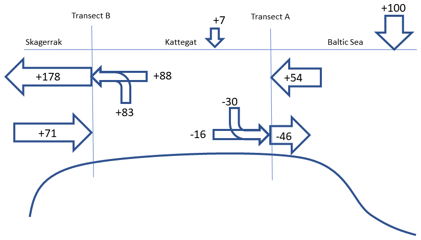
Figure 11 Change in volume fluxes in m³ s⁻¹ for an increase in freshwater input to the Baltic Sea of $\mathrm{\Delta }{Q}_{\mathrm{f}}=\mathrm{100}{\mathrm{m}}^{\mathrm{3}}{\mathrm{s}}^{-\mathrm{1}}$ averaged over the period 1990–2017. The arrows are described in the Fig. 10 caption. The fluxes are based on the differences between runs RP+ and RP- but normalized to represent an increase in Q_f of 100 m³ s⁻¹.

Figure 12 shows the probability density functions (pdf) for inflows and outflows through the sill transect for the hindcast and changed runoff and precipitation cases. It is seen that the changed freshwater basically shifts the pdf towards larger or smaller inflows while maintaining the same shape.

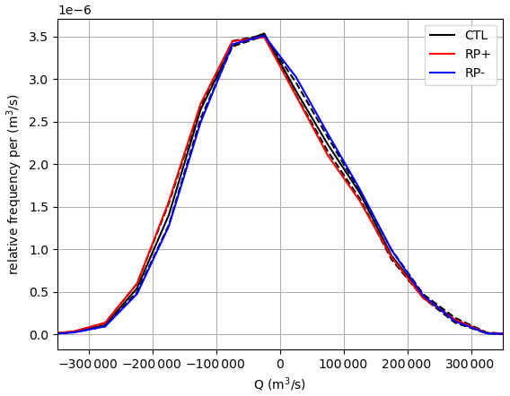
Figure 12 Probability density function for inflows (net inflows at each time step) for the hindcast run and the RP+ and RP- runs at the sill transect. Dashed lines show the frequency distributions for the hindcast run with 4387 m³ s⁻¹ added and subtracted from the hindcast run time series.

Since the curve is almost symmetric around zero, though shifted somewhat towards the negative side, shifting the curve laterally causes almost the same decrease or increase on the positive side as the increase or decrease on the negative side. This explains why the changes in inflows and outflows (Fig. 11) are of about the same magnitude.

The dashed lines in Fig. 12 are pdfs obtained from the hindcast run time series with an addition or subtraction of a constant volume flux corresponding to the mean change in Q_f for the RP+ and RP- cases. These are quite similar to the corresponding RP+ and RP- curves. This indicates that the changed in- and outflows are basically caused by a shift up or down of the time series with the mean change in Q_f. This also means that there is a larger relative change to intermediate strength in- and outflows than to low and high strength in- and outflows where the change in frequency is small when changing the volume flux with the change in Q.

One way to explain that an increased input of freshwater causes a more or less constant change to the fluctuating inflows is that they cause a raised sea level relative to the reference situation, Fig. 13, which causes an extra outward barotropic flow. Similarly, a decreased input of freshwater will cause a lowered sea level relative to the reference situation and therefore smaller outward barotropic flows and increase inward barotropic flows.

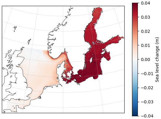
Figure 13 Mean sea level difference (m) between run RP+ and CTL for the years 1990–2017.

4 Summary and discussion

The sensitivity of the Baltic Sea steady state salinity was investigated with a series of 57 year runs with a regional ocean model for the Baltic and North Sea, consisting of a hindcast run, and perturbations of that with respect to boundary salinity and freshwater forcing.

A second order polynomial of the Baltic Sea mean steady state salinity in terms of the variables boundary salinity and freshwater forcing was constructed. This provides means of quickly assessing the importance of changes of North-East Atlantic salinities and freshwater forcing for Baltic Sea salinities, e.g. based on global projections and/or regionally downscaled atmospheric and hydrological projections. Similar polynomials can be constructed for sensitivity of other parameters to these variables based on the present run. The results showed a large and non-linear sensitivity to precipitation and runoff, whereas the response to boundary salinity was linear. The response of the Baltic Sea to boundary salinity may be seen as small or large depending on perspective. Only 36 % of the boundary salinity change was seen in the Baltic Sea, but since the salinity of the Baltic Sea is only about 22 % of that in the North Sea, the relative change is actually larger in the Baltic Sea than in the North Sea.

Total exchange flow analysis was used to analyze inflows and outflows through two transects located over the sills and in the northern end of Kattegat, as well as the water mass transformation within Kattegat and the Belt Sea. It was found that the inflowing water through the sill transect consisted of 36 % Skagerrak water (inflow water through the northern Kattegat transect) and 64 % outflowing Baltic Sea water. When modifying runoff and precipitation, this mixture remained relatively constant.

When increasing precipitation and runoff to the Baltic Sea, the net outflow though the entrance will increase with about the same amount. This can result in either increased outflows and/or decreased inflows. In our model study, 54 % of the runoff increase resulted in increased outflows of volume through the sill transect, whereas 46 % resulted in decreased inflows of volume. One way to explain this change is that the increased freshwater input causes a higher sea level in the Baltic Sea, and therefore a net change in sea level gradients over the inflow region which causes a change to the barotropic flows. With the large-amplitude fluctuations in in- and outflows taking place in the inflow region, such a more or less constant net change to the barotropic flows contributes almost equally to increased outflows and decreased inflows.

The above results show that the sensitivity of the Baltic Sea mean salinity to increased freshwater forcing is caused both by decreased inflow volume fluxes and by recirculation of the outflowing Baltic Sea water that causes fresher inflows. In a steady state, following Knudsen (1900), the net flow of salt is zero and the net outflow of volume is equal to the net input of freshwater. To this can be added the result of the present work that the salinity of inflows through the sill transect can be written as

$$\begin{array}{}\text{(22)}& S_{\text{in}}=\mathit{\alpha }{S}_{\mathrm{0}}+(\mathrm{1}-\mathit{\alpha })S_{\text{out}},\end{array}$$

where S₀ is the salinity of the inflowing water from Skagerrak, S_out is the salinity of outflowing water from the Baltic Sea through the sill transect, and α is the amount of Skagerrak water in the inflowing water, α=0.36 according to the results of this study. Using Eq. (22) in combination with the Knudsen relations give the following equation for the salinity of outflowing water from the Baltic Sea

$$\begin{array}{}\text{(23)}& S_{\text{out}}=\mathit{\alpha }{S}_{\mathrm{0}}{\displaystyle \frac{Q_{\text{in}}}{Q_{\mathrm{f}}+\mathit{\alpha }{Q}_{\text{in}}}}.\end{array}$$

Assuming that α andS₀ are independent of Q_f, the derivative with respect to S_out can be written as

$$\begin{array}{}\text{(24)}& {\displaystyle \frac{\partial S_{\text{out}}}{\partial Q_{\mathrm{f}}}}=\mathit{\alpha }{S}_{\mathrm{0}}{\displaystyle \frac{-Q_{\text{in}}+\mathit{\beta }{Q}_{\mathrm{f}}}{(Q_{\mathrm{f}}+\mathit{\alpha }{Q}_{\text{in}}{)}^{\mathrm{2}}}}\end{array}$$

where $\mathit{\beta }=\frac{\partial Q_{\text{in}}}{\partial Q_{\mathrm{f}}}=-\mathrm{0.46}$ according to the results above. With S₀=33.5 psu (calculated with the total exchange flow analysis for the CTL case), $Q_{\text{in}}=\mathrm{13}\mathrm{500}{\mathrm{m}}^{\mathrm{3}}{\mathrm{s}}^{-\mathrm{1}}$ (Fig. 10), and Q_f=15 700 m³ s⁻¹ this gives $\partial S_{\text{out}}/\partial Q_{\mathrm{f}}=-\mathrm{5.91}\times {\mathrm{10}}^{-\mathrm{4}}$ psu s m⁻³ or 1.05 % decrease in outflow salinity for 1 % increase in Q_f. The finite difference derivative based on mean outflow salinities and net freshwater input of the RP+ and RP- experiments is $\mathrm{\Delta }{S}_{\text{out}}/\mathrm{\Delta }{Q}_{\mathrm{f}}=-\mathrm{5.23}\times {\mathrm{10}}^{-\mathrm{4}}$ psu s m⁻³ or 0.93 % decrease in outflow salinity for 1 % increase in Q_f. The two estimates are similar enough to support the assumptions behind the simplified steady state expressions, keeping in mind that α is not perfectly constant, that the runs are not totally in steady state, and that diffusive transports across the transects are not considered in the total exchange flow analysis.

With β=0, i.e. with no decrease in inflow for increasing freshwater input, Eq. (24) gives $\partial S_{\text{out}}/\partial Q_{\mathrm{f}}=-\mathrm{3.85}\times {\mathrm{10}}^{-\mathrm{4}}$ psu s m⁻³ which is 65 % of the value with $\mathit{\beta }=-\mathrm{0.46}$. This means that 35 % of the sensitivity of Baltic Sea salinity to freshwater input can be attributed to decreased inflows alone.

If we instead assume that the inflow salinity at the sill transect is constant (i.e. not governed by Eq. 22), the outflow salinity can be found directly from the Knudsen relations as

$$\begin{array}{}\text{(25)}& S_{\text{out}}={\displaystyle \frac{S_{\text{in}}{Q}_{\text{in}}}{Q_{\mathrm{f}}+Q_{\text{in}}}}.\end{array}$$

with the partial derivative with respect to Q_f being

$$\begin{array}{}\text{(26)}& {\displaystyle \frac{\partial S_{\text{out}}}{\partial Q_{\mathrm{f}}}}=S_{\text{in}}{\displaystyle \frac{-Q_{\text{in}}+\mathit{\beta }{Q}_{\mathrm{f}}}{(Q_{\mathrm{f}}+Q_{\text{in}}{)}^{\mathrm{2}}}}.\end{array}$$

With a constant inflow salinity of 17.6 psu calculated with the total exchange flow analysis for the steady state reference run, this gives $\partial S_{\text{out}}/\partial Q_{\mathrm{f}}=-\mathrm{4.28}\times {\mathrm{10}}^{-\mathrm{4}}$ psu s m⁻³, which is 72 % of the full sensitivity. This means that 28 % of the sensitivity can be attributed to decreased inflow salinity alone, i.e. by recirculation of outflow water in the Kattegat and Belt Sea region.

The sensitivity with both constant inflow volume flux and constant inflow salinity, i.e. caused by dilution inside the Baltic Sea alone, can be determined from Eq. (26) with β=0 and is 47 % of the total sensitivity. The combined influence of reduced inflow volume fluxes and reduced inflow salinities due to recirculation in the entrance region therefore is 53 % of the total sensitivity. These simplified estimates based on results from the full sensitivity study cannot be expected to give the exact picture, but they do show that dilution inside the Baltic Sea, inflow changes, and inflow salinity changes due to recirculation in the entrance region are all important contributions to the Baltic Sea sensitivity to freshwater forcing. These results do give a new picture of the factors influencing Baltic Sea salinity sensitivity to freshwater forcing. For example, Radtke et al. (2020) find that only about 25 % of the salinity sensitivity is caused by direct dilution, and Meier et al. (2023) although they find that both direct dilution and changing inflows are important for low-frequency salinity variability, they do not separate the influences of inflow volume and inflow salinity, and they do not quantify the various contributions. It is also worth mentioning that both of these studies focus on the low-frequency variability rather than the steady stated change that we are approaching.

A sensitivity of about 1 % salinity decrease for a 1 % inflow increase is in the same order of magnitude but in the low end of earlier estimates (e.g. Stigebrandt, 1983; Stigebrandt and Gustafsson, 2003; Meier and Kauker, 2003) which are generally in the range 1.15 %–1.5 %. These studies have explained the sensitivity in terms of other processes, including geostrophic control in the Arkona basin (Meier and Kaufer, 2003), and geostrophic control of the outflowing Kattegat water combined with assumptions on how this relates to inflow salinities as well as reduced inflow volumes with increased freshwater input (Stigebrandt and Gustafsson, 2003). The present results provide a simpler framework for describing the salinity sensitivity, although work is still needed to understand why the fractions of North Sea and Baltic Sea water remain relatively constant, when freshwater forcing changes.

The sensitivity of Baltic Sea outflow salinity to North Sea salinity can easily be determined from Eq. (23) as

$$\begin{array}{}\text{(27)}& {\displaystyle \frac{\partial S_{\text{out}}}{\partial S_{\mathrm{0}}}}=\mathit{\alpha }{\displaystyle \frac{Q_{\text{in}}}{Q_{\mathrm{f}}+\mathit{\alpha }{Q}_{\text{in}}}},\end{array}$$

which gives 0.24. This is smaller than 0.37 which is found from the finite difference gradient of outflow salinities based on the SB+ and SB- runs, which may again have to do with the lack of totally steady conditions. Note that according to this expression the relative change in the Baltic Sea is expected to be equal to the relative change in the North Sea. It is interesting to note that Stigebrandt (1983) found a sensitivity of 0.3 with a model much simpler than our regional model but also much more complex than Eqs. (23) and (25).

The validity of the presented results depends on the validity of the model. The model has shown a good representation of historical variability of salinities in the Baltic Sea in response to varying freshwater input and atmospheric forcing, which lends some confidence in the conclusions.

The next step is to look further into the sensitivity of Baltic Sea salinities to sea level rise. With sea level rise, both the recirculation of water in the Kattegat and Belts Sea region and the inflow strength will change. Both the fraction of Skagerrak water in the inflows and the inflows themselves will increase. It is uncertain to what degree the present model is able to describe these changes, both with regard to the basic coarse resolution of the bathymetry and straits where small cross-sectional changes may not be well represented, and with respect to resolving important physical processes governing the changes in inflow strength and mixing (e.g. Arneborg, 2016; Haid et al., 2020). Given the large importance of recirculation and mixing in the entrance region for Baltic Sea salinity, it will be necessary to look further into how well the model and possibly higher-resolution versions of the model represent water mass transformation processes in this region.