Modelling seawater pCO₂ and pH in the Canary Islands region based on satellite measurements and machine learning techniques

Recent advancements in remote sensing systems, combined with new machine-learning model-fitting algorithms, have enabled the estimation of seawater carbon dioxide partial pressure (pCO_2,sw) and pH (pH_T,is) in the waters around the Canary Islands (13–19° W; 27–30° N). Continuous time-series data collected from moored buoys and Voluntary Observing Ships (VOS) between 2019 and 2024 were used to train and validate the models, providing a robust observational basis for satellite-derived estimates.

Among all models tested, bootstrap aggregation (bagging) performed best, achieving an RMSE of 2.0 µatm (R²>0.99) for pCO_2,sw and 0.002 for pH_T,is. Multilinear regression (MLR), neural networks (NN) and categorical boosting (CatBoost) also showed good predictive skill, with RMSE values between 5.4 and 10 µatm for pCO_2,sw (360–481 µatm) and 0.004–0.008 for pH_T,is (7.97–8.07). Using the most reliable model, we identified an increasing trend in pCO_2,sw of 3.51±0.31 µatm yr⁻¹, exceeding the atmospheric CO₂ growth rate (2.3 µatm yr⁻¹), alongside an acidification trend of −0.003 ± 0.001 yr⁻¹.

Over the 2019–2024 period, rising atmospheric CO₂ and increasing sea surface temperatures (reaching up to 0.2 °C yr⁻¹ during the unprecedented 2023 marine heatwave) likely contributed to these trends. The Canary Islands region shifted from a weak CO₂ source (0.90 Tg CO₂ yr⁻¹) in 2019 to 4.5 Tg CO₂ yr⁻¹ in 2024. After 2022, eastern sites that previously acted as annual CO₂ sinks became net sources.

1 Introduction

Anthropogenic emissions of carbon dioxide (CO₂) from fossil fuel combustion, cement production and land-use change (Doney et al., 2009; Le Quéré et al., 2009; Siegenthaler and Sarmiento, 1993; Zeebe, 2012) since the First Industrial Revolution have sharply increased atmospheric concentrations of this trace gas. This rise is partly mitigated by uptake from terrestrial vegetation and the oceans (Friedlingstein et al., 2025). The North Atlantic Ocean is reported as one of the major oceanic CO₂ sinks in the Northern Hemisphere, absorbing 2.6 ± 0.4 Pg CO₂ yr⁻¹. This is equivalent to ∼ 25 % of the oceanic anthropogenic CO₂ sink, based on 18 years of observations (Gruber et al., 2002).

Recent research has placed increasing emphasis on quantifying oceanic CO₂ uptake and its impact (e.g., Bange et al., 2024; Gregor et al., 2024). A common approach involves using regression models to estimate surface ocean CO₂ partial pressure (pCO_2,sw) from environmental variables. However, these models often fall short in capturing the complexity of dynamic regions such as coastal zones and continental shelves (Sun et al., 2021). These areas exhibit intense physical and biogeochemical activity, driven by high rates of primary production, carbon burial, organic matter recycling, and calcium carbonate deposition (Boehme et al., 1998; Borges et al., 2005; Gattuso et al., 1998). Despite their importance, these regions remain poorly constrained in global carbon budgets and air-sea CO₂ flux estimates (Dai et al., 2022).

Pioneering studies by Borges et al. (2005) and Cai et al. (2006) provided the first global assessments of coastal CO₂ fluxes, emphasizing strong spatial heterogeneity and functional diversity of coastal ecosystems in the global carbon cycle. More recent studies indicate that coastal regions act as significant CO₂ sinks, with global ingassing estimates of 0.54–1.47 Pg CO₂ yr⁻¹ (Cao et al., 2020; Laruelle et al., 2014), though updated assessments suggest lower rates (Dai et al., 2022; Regnier et al., 2022; Resplandy et al., 2024; Roobaert et al., 2019).

At large latitudinal scale, sea surface temperature (SST) is a primary driver of surface ocean pCO_2,sw, often expressed as CO₂ fugacity (fCO_2,sw), which accounts for non-ideal gas behaviour due to molecular interactions and is typically slightly lower than pCO₂ (Wanninkhof et al., 2022). At smaller spatial scales (within latitudinal bands), additional drivers such as upwelling-driven CO₂ supply and biological uptake of dissolved inorganic carbon (C_T) become relevant (e.g., Laruelle et al., 2014).

The pCO_2,sw is governed by four interconnected processes: thermodynamic forcing, biological activity, physical mixing, and air-sea CO₂ exchange (Fennel et al., 2008; Ikawa et al., 2013). One or two of these processes typically dominating in any given region (Bai et al., 2015). The thermodynamic component is primarily influenced by the SST and sea surface salinity (SSS), which determine CO₂ solubility (Weiss, 1970) and carbonic acid dissociation constants (e.g., Lueker et al., 2000). Biological effects can be approximated using satellite-derived chlorophyll a (Chl a) and the diffuse attenuation coefficient of downwelling irradiance at 490 nm (Kd₄₉₀) (Bai et al., 2015; Chen et al., 2019; Lohrenz et al., 2018). Vertical mixing processes, particularly those enriching surface waters with CO₂ from deeper layers, are commonly parameterised using mixed-layer depth (MLD) (Chen et al., 2019). Additionally, the continuous rise in pCO_2,atm, which drives the air-sea CO₂ gradient, must be considered in long-term assessments.

Satellite remote sensing provides broad spatiotemporal coverage for surface pCO_2,sw estimation (Chen et al., 2019). In the open settings with relatively variability, satellite-based estimates achieve RMSE < 17 µatm. Errors exceed 90 µatm in coastal waters due to increased complexity in physical and biogeochemical processes (Lohrenz et al., 2018; Sun et al., 2021). Traditional empirical approaches include multilinear (MLR) and nonlinear regression (MNR). Shadwick et al. (2010) applied MLR to the Scotian Shelf (R²=0.81; SE = 13 µatm). Signorini et al. (2013) reported RMSE of 22.4–36.9 µatm along the U.S. East Coast. Chen et al. (2016) developed a satellite-based model for the West Florida Shelf with RMSE < 12 µatm.

Machine learning (ML) approaches, such as neural networks (NN), random forests and CatBoost, have improved prediction skills. Lefèvre and Taylor (2002) reported NN residuals of 3–11 µatm in the subpolar gyre. Telszewski et al. (2009) obtained RMSE of 11.6 µatm in the North Atlantic. Sun et al. (2021) used CatBoost to reach RMSE of 8.25 µatm (R²=0.946). Gregor et al. (2024) applied ML with target transformation at the global scale (1982–2022), resolving 15 % more CO₂ flux (FCO₂) variance than traditional methods.

In coastal studies, Jo et al. (2012) used NN with SST and Chl a in the South China Sea (RMSE = 6.9 µatm; r=0.98). Duke et al. (2024) showed that nearshore outgassing reduces net flux in the Northeast Pacific. Roobaert et al. (2024) highlighted strong seasonal FCO₂ variability driven by open-ocean and intracoastal exchanges. Wu et al. (2024) applied ML in the Gulf of Mexico, estimating 1.5 TgC yr⁻¹ of CO₂ uptake, though long-term trends remained uncertain.

The present study focuses on the coastal Canary Islands basin (27.0–30° N; 13.0–19° W) (Fig. 1), located in oligotrophic waters of the eastern subtropical North Atlantic gyre (Pelegrí et al., 1996). The region is influenced by the Canary Current and trade winds, which generate mesoscale eddies. Despite low surface Chl a concentrations, primary productivity may increase due to upwelling filaments from NW Africa, eddies, and dust fertilization (Davenport et al., 1999). Marine heatwaves (MHWs) are intensifying under climate change (Frölicher and Laufkötter, 2018; Hobday et al., 2016; Holbrook et al., 2019). Varela et al. (2024) reported that 2023 was the warmest year in the Canary Upwelling System since 1982, with widespread record SST, likely affecting CO₂ dynamics.

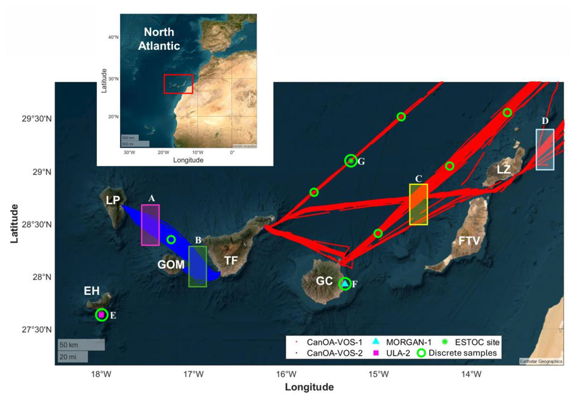
Figure 1 Map of the Canary Islands showing the CanOA-VOS tracks (CanOA-VOS-1 Jona Sophie, in red; and CanOA-VOS-2 Benchijigua Express, in blue), the locations of the moored oceanographic buoys (MORGAN-1, cyan triangle; ULA-2, purple square), the ESTOC site (green star), and green circles indicate discrete sampling locations. The positions of sites A–F are also indicated, with site E corresponding to the ULA-2 buoy, site E to the MORGAN-1 buoy, and site G to the ESTOC site. The island acronyms are included (EH: El Hierro, LP: La Palma, GOM: La Gomera, TF: Tenerife, GC: Gran Canaria, FTV: Fuerteventura, LZ: Lanzarote). The figure was created with Matlab (version 2023b) software using the geoplot function with a satellite basemap. Basemap: Esri World Imagery (satellite imagery), © Esri and its data providers.

Long-term observations reveal a consistent rise in surface pCO_2,sw in this region. Takahashi et al. (2009) estimated an increase of 1.8 ± 0.4 µatm yr⁻¹ for the North Atlantic (1972–2006). Bates et al. (2014) reported 1.92 ± 0.92 µatm yr⁻¹ (1996–2012) at the ESTOC (European Station for Timeseries in the Ocean Canary Islands) site, with pH_T,is (pH in total scale and at in situ temperature) decreasing by −0.0018 ± 0.0002 yr⁻¹. More recently, González-Dávila and Santana-Casiano (2023) reported pCO_2,sw increasing by 2.1 ± 0.1 µatm yr⁻¹ and pH_T,21 decreasing by −0.002 ± 0.0001 yr⁻¹ in the upper 100 m (1995–2023), around 20 % faster than rates for 1995–2010.

The aim of this study was to develop and validate a machine-learning algorithm to estimate pCO_2,sw, pH_T,is and FCO₂ in the Canary Basin (NE Atlantic) using satellite-derived environmental variables and a high-resolution time series of pCO_2,sw observations from voluntary observing ships (VOS) and moored oceanographic buoys.

2 Material and methods

2.1 Data

2.1.1 In situ observations

The observational dataset was compiled using measurements from Surface Ocean Observation Platforms (SOOPs) installed on Volunteer Observing Ships (VOS) and moored oceanographic buoys (Fig. 1; Table S1 in the Supplement). Two VOS collect continuous underway data along their routine shipping routes:

1. The CanOA-VOS-1 on board the Jona Sophie (formerly Renate P.) operated in Spain by Nisa Marítima and owned by Reederei Stefan Patjens GmbH & Co. KG. This cargo vessel services the eastern Canary Islands between Tenerife (TF; 28.4867° N, 16.2284° W), Gran Canaria (GC; 28.1319° N, 15.4185° W) and Lanzarote (LZ; 28.9682° N, 13.5294° W) and continues northeast of Lanzarote in route to Barcelona (Spain). Seawater is sampled from a depth of 7 m. CanOA-VOS-1 contributes to the Spanish component of Integrated Carbon Observation System (ES-SOOP-CanOA, ICOS-ERIC; https://www.icos-cp.eu/, last access: 22 January 2026) since 2021 and has been classified as an ICOS Class 1 Ocean Station.

2. The CanOA-VOS-2 on board Benchijigua Express, operated and owned by Fred Olsen Express, covering the western islands between a second port in Tenerife (TF; 28.0486° N, 16.7163° W), La Gomera (GOM; 28.0859° N, 17.1090° W) and La Palma (LP; 28.6751° N, 17.7666° W). The seawater intake is located at 5 m depth.

In addition, two coastal oceanographic buoys record surface data at 1 m depth:

1. MORGAN-1 (Gando, Gran Canaria, 27.9296° N, 15.3646° W; González et al., 2024).

2. ULA-2 (El Hierro, 27.6350° N, 17.9964° W).

All autonomous underway monitoring and data acquisition follows the quality-control procedures recommended by Pierrot et al. (2009). A detailed description of equipment can be found in Curbelo-Hernández et al. (2021, 2022) and in the Supplement. The number of used observations is listed in Table S1 in the Supplement.

Discrete samples of total alkalinity (A_T) and total inorganic carbon (C_T) were collected on board by a scientist on a transect every three months on the same seawater intake line used by the underway system, ensuring coverage across seasons and sampling sites (Fig. 1). Analyses were performed using a VINDTA 3C (Marianda™) following Mintrop et al. (2000). Calibration was carried out using Certified Reference Material (CRMs; provided by Andrew Dickson, Scripps Institution of Oceanography), with an accuracy of ± 1.5 µmol kg⁻¹ for A_T and ± 1.0 µmol kg⁻¹ for C_T. Differences between pCO_2,sw (converted from measured xCO_2,sw; for method see below) and discrete pCO_2(AT,CT) (CO₂sys.V2.1.xls, set of carbonic acid constants from Lueker et al., 2000, n=66) were 4 ± 4 µatm for the GO8050 and 7 ± 5 µatm for the ProCV system. A correction factor was applied to account for these offsets.

For regional comparison, seven locations were defined across the archipelago (Fig. 1): Site A, along the LP-GOM route (17.5 ± 0.05° W); Site B, along the GOM-TF route (16.95 ± 0.05° W). Site C, at the intersection of multiple ship routes (14.65 ± 0.05° W); Site D, near the NW African coast along the LZ-Iberian Peninsula route (13.2 ± 0.05° W); Site E, at the ULA-2 buoy near El Hierro; Site F at the MORGAN-1 buoy at Gando bay (GC); and Site G at the ESTOC site.

2.1.2 Satellite data

Satellite-derived SST, Chl a, Kd₄₉₀, MLD data were used to develop the pCO_2,sw and pH_T,is forecast models, while wind speed was incorporated for FCO₂ calculation. All satellite products were obtained from the Copernicus Marine Environmental Monitoring Service (CMEMS; https://marine.copernicus.eu/access-data, last access: 27 May 2025). Wind speed data were retrieved from the Agencia Estatal de Meteorología (AEMET; AEMET Open Data, https://opendata.aemet.es/centrodedescargas/productosAEMET, last access: 8 October 2025). Wind measurements were taken La Palma Airport (33 m), La Gomera Airport (15 m), Fuerteventura Airport (25 m), Lanzarote Airport (14 m), Gran Canaria Airport (24 m), and El Hierro Airport (32 m), corresponding to sites A–F of the study area. Wind speeds were standardised to 10 m height following Allen et al. (1998). All variables were processed and matched in time and space to the observational records, and daily means were used for model calibration and validation. The full daily dataset was then applied to generate the surface marine carbonate system variables in the Canary Islands.

Satellite-derived products carry inherent uncertainties associated with remote sensing retrievals. For the used CMEMS products, mean uncertainties were 0.62 °C for SST and 0.485 mg m⁻³ for Chl a. Their contribution to prediction error was assessed during model validation through comparison with coincident in situ measurements.

2.2 Variable determination and computational methods

The raw data were processed using MATLAB^® R2019b and Python 3.13.6 (2023). For the VOS dataset, xCO_2,sw measurement from the GO8050 system were calibrated using a four-standard procedure, after filtering data points collected near ports where seawater CO₂ concentrations may be influenced by local activities. Quality control included applying minimum flow thresholds of 2.5 L min⁻¹ for the seawater line and 50 mL min⁻¹ for the LICOR^© gas flow.

The partial pressure of CO₂ in seawater (pCO_2,eq) was calculated from corrected dry xCO₂ (Dickson et al., 2007). Values from both VOS routes were subsequently adjusted to intake temperature to account for differences between the thermosalinograph/equilibrator temperature and SST (Takahashi et al., 1993). Fugacity (fCO_2,sw) was then computed from pCO_2,sw for both VOS and buoy datasets (Dickson et al., 2007). Discrete samples analysed for A_T using the VINDTA 3C were used to determine an A_T-SSS relationship for the study region (n=66), consistent with that previously reported for the ESTOC site (González Dávila et al., 2010). The normalised A_T (NA${}_{\mathrm{T}}=A_{\mathrm{T}}/\text{SSS}\times \mathrm{35}$) was 2290±3 µmol kg⁻¹, significant at the 99 % confidence level (p-value < 0.01; r²=0.96), with no evidence of seasonal variability, in agreement with long-term ESTOC observation (González Dávila et al., 2010). This relationship was applied to compute total scale pH_T,is(A_T(SSS), fCO_2,sw) for the Canary Region (González Dávila et al., 2010). All process variables were averaged to a daily resolution.

Daily mean atmospheric xCO_2,atm was obtained from onboard atmospheric measurements and compared with records from the World Meteorological Organisation (WMO) Izaña Atmospheric Observatory (AEMET, 2024) in Tenerife (28°18^′ N, 16°29^′ W), due to potential contamination by ship operations. Winter maxima were similar between datasets (±1.5 µatm), while late summer minima at Izaña were on average 3 µatm higher than values measured at the ship's 10 m inlet. As in situ coverage was limited and the Izaña record provided a longer continuous series, the Izaña xCO_2,atm dataset was adopted for this study. Atmospheric xCO_2,atm was converted to pCO_2,atm (Dickson et al., 2007).

The flux of CO₂, FCO₂, was determined using Eq. (1):

$$\begin{array}{}\text{(1)}& {\mathrm{FCO}}_{\mathrm{2}}=\mathrm{0.24}kS\mathrm{\Delta }p{\mathrm{CO}}_{\mathrm{2}}\end{array}$$

where 0.24 is the conversion factor to express the flux in mmol m⁻² d⁻¹, S is the solubility of CO₂ in seawater (Weiss, 1970), ΔpCO₂ is pCO${}_{\mathrm{2},\mathrm{sw}}-p$CO_2,atm and k is the gas transfer rate determined using the Wanninkhof (2014) parameterization (Eq. 2):

$$\begin{array}{}\text{(2)}& k_{\mathrm{Wan}}=\mathrm{0.251}{u}^{\mathrm{2}}(Sc/\mathrm{650}{)}^{-\mathrm{0.5}}\end{array}$$

where u is the wind speed (m s⁻¹) and Sc is the Schmidt number.

Equation (1) was applied to the daily modelled data. Daily fluxes were averaged to provide monthly fluxes, which are reported as daily average value for each month (mmol m⁻² d⁻¹).

Each physicochemical variable y (including pCO_2,atm and fCO_2,atm) was fitted to a harmonic function (Eq. 3, where t is the year fraction for each observation). Seasonal anomalies were obtained by adding the residuals between observed values and those predicted by Eq. (3) to the constant term a in Eq. (3), representing the mean value of y for the study period. Interannual trends were then estimated using Eq. (4) applied to the deseasonalised time series. Although the length of the dataset is relatively short (5–6 years), the use of detrended seasonal anomalies minimizes end-effects and improves the robustness of the trend estimation.

$$\begin{array}{}\text{(3)}& {\displaystyle }\begin{array}{rl}y& =a+c\cdot \sin \left(\mathrm{2}\mathit{\pi }t\right)+d\cdot \cos \left(\mathrm{2}\mathit{\pi }t\right)+e\cdot \sin \left(\mathrm{4}\mathit{\pi }t\right)\\ & +\cos \left(\mathrm{4}\mathit{\pi }t\right)\end{array}\text{(4)}& {\displaystyle }\begin{array}{rl}y& =a+b\cdot \left(t-\mathrm{2019}\right)+c\cdot \sin \left(\mathrm{2}\mathit{\pi }t\right)+d\cdot \cos \left(\mathrm{2}\mathit{\pi }t\right)\\ & +e\cdot \sin \left(\mathrm{4}\mathit{\pi }t\right)+\cos \left(\mathrm{4}\mathit{\pi }t\right)\end{array}\end{array}$$

2.3 Model fitting and statistical treatment

Statistical analyses were conducted using R (R Core Team, 2019). Machine-learning methods were used to fit the different models. The dataset was initially partitioned into training (80 %) and validation (20 %) subsets, with allocation performed randomly at the cruise level to avoid temporal bias. This random split was repeated for each model run to ensure representative sampling. Once model performance had been evaluated, the complete dataset was used to provide the optimal model parameters.

The simplest fitted model was a multiple linear regression (MLR), defined analytically in Eq. (5):

$$\begin{array}{}\text{(5)}& \begin{array}{rl}p{\mathrm{CO}}_{\mathrm{2},\mathrm{sw}}& =p_{\mathrm{0}}+\widehat{\mathit{\alpha }}p{\mathrm{CO}}_{\mathrm{2},\mathrm{atm}}\left(\mathrm{\mu }\mathrm{atm}\right)+\widehat{\mathit{\beta }}\mathrm{SST}\left(\mathrm{°}\mathrm{C}\right)\\ & +\widehat{\mathit{\gamma }}\mathrm{Chl}\left(\mathrm{mg}{\mathrm{m}}^{-\mathrm{3}}\right)+\widehat{\mathit{\delta }}{K}_{\mathrm{d},\mathrm{490}}\left({\mathrm{m}}^{-\mathrm{1}}\right)\\ & +\widehat{\mathit{\epsilon }}\mathrm{MLD}\left(\mathrm{m}\right)+\mathit{\vartheta }\end{array}\end{array}$$

where $\widehat{\mathit{\alpha },}\widehat{\mathit{\beta }},\widehat{\mathit{\gamma }},\widehat{\mathit{\delta }}$ and $\widehat{\mathit{\epsilon }}$ are the estimated coefficients for each predictor and ϑ the residuals. The same equation (without the $\widehat{\mathit{\alpha }}$ term) was used to model pH_T,is dependence.

Three machine-learning techniques were used: neural network (NN; Wang, 2003), categorical boosting (CatBoost; Dorogush et al., 2018; Prokhorenkova et al., 2018; Qian et al., 2023) and bootstrap aggregation (bagging; Breiman, 1996).

These approaches are widely employed in environmental modelling and provide complementary approaches for improving predictive accuracy by reducing variance and capturing nonlinear relationships.

CatBoost is a gradient-boosting algorithm that constructs decision trees sequentially and efficiently handles categorical features, minimising information loss. Its ordered-boosting framework reduces prediction shift associated with gradient bias (Dorogush et al., 2018; Prokhorenkova et al., 2018; Qian et al., 2023; Sun et al., 2021).

Neural Networks (NN) are flexible nonlinear models inspired by the human brain, capable of capturing complex relationships between inputs and outputs (Wang, 2003). These methods are composed of interconnected neurons arranged in layers: an input layer representing predictors, one or more hidden layers, and an output layer producing the final prediction.

Bootstrap aggregation (bagging) is an ensemble technique that improves predictive robustness by generating multiple versions of a model trained on different bootstrap samples of the dataset (Breiman, 1996). Predictions are then averaged to reduce variance and prevent overfitting, making the overall model more stable and reliable.

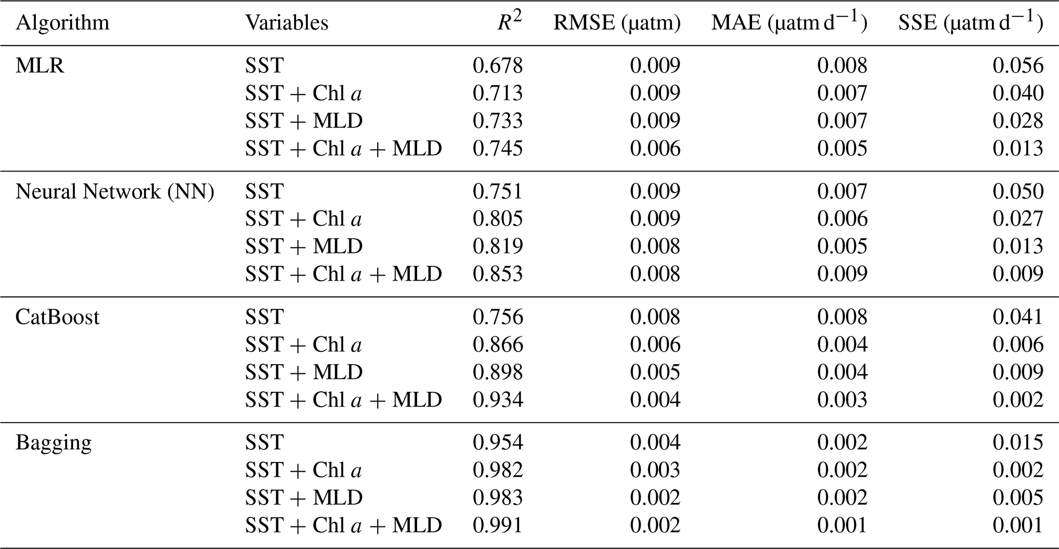
Model performance was assessed using the validation dataset through the coefficient of determination (R²), root mean square error (RMSE; Eq. 6), mean absolute error (MAE; Eq. 7), and daily sum of squared errors (SSE; Eq. 8).

$$\begin{array}{}\text{(6)}& {\displaystyle }\mathrm{RMSE}=\sqrt{{\displaystyle \frac{{\sum }_{i=\mathrm{1}}^N{\left(p{\mathrm{CO}}_{\mathrm{2},i}-\widehat{p{\mathrm{CO}}_{\mathrm{2},i}}\right)}^{\mathrm{2}}}{N}}}\text{(7)}& {\displaystyle }\mathrm{MAE}={\sum }_{i=\mathrm{1}}^N\left|p{\mathrm{CO}}_{\mathrm{2},I}-\widehat{p{\mathrm{CO}}_{\mathrm{2},i}}\right|/d\text{(8)}& {\displaystyle }\mathrm{SSE}={\sum }_{i=\mathrm{1}}^N{\left(p{\mathrm{CO}}_{\mathrm{2},I}-\widehat{p{\mathrm{CO}}_{\mathrm{2},i}}\right)}^{\mathrm{2}}/d\end{array}$$

where pCO_2,i and $\widehat{p{\mathrm{CO}}_{\mathrm{2},i}}$ are the observed and modelled pCO₂, N is the number of observations and d is the number of days in the dataset.

The Akaike information criterion corrected for a finite dataset (AIC_c) was determined using Eq. (9). It evaluates the balance between goodness-of-fit and model complexity (i.e., number of predictors). Among competing models, the one with the lowest AIC_c is considered the most appropriate.

$$\begin{array}{}\text{(9)}& {\mathrm{AIC}}_{\mathrm{c}}=\mathrm{2}k-\mathrm{2}\ln \left(L\right)+{\displaystyle \frac{\mathrm{2}{k}^{\mathrm{2}}+\mathrm{2}k}{n-k-\mathrm{1}}}\end{array}$$

where k is the number of parameters involved in the model, ln (L) is the log-likelihood for the predicted model and n is the number of observations.

To estimate the coefficients of each seasonal model and determine confidence intervals, two assumptions were tested: (1) normality of residuals, assessed using the two-Welch Shapiro-Wilk test (α=0.05) and quantile-quantile plots, and (2) homogeneity of residual variance (homoscedasticity), assessed graphically. When the normality assumption was not met, bootstrapping was used to determine confidence intervals. Model comparisons were performed using analysis of covariance (ANCOVA) and analysis of variance (ANOVA) to detect significant differences at α=0.05.

3 Results

The observational data enabled the construction of a database for modelling the behaviour of pCO_2,sw and pH_T,is in the Canary Basin. To characterise the measured and satellite-derived parameters used in this study, Table 1 summarises their seasonal mean and standard deviations for each observation system. In situ SST (Fig. 2) showed a clear seasonal cycle, with maximum temperatures in summer (July–September) and minima in winter (January–March). The highest SST occurred in the westernmost sector of the archipelago (between La Palma and Tenerife), averaging ∼ 1 °C warmer than the eastern sector (between Gran Canaria and Lanzarote). A similar seasonal and longitudinal pattern was observed for pCO_2,sw and pH_T,is (Table 1). Seasonal and annual SST means derived from in situ and satellite observations differed by ∼ 0.15 °C on average.

Table 1 Seasonal mean and standard deviations of observational data (pCO_2,sw and SST) and satellite-derived data (SST, Chl a, Kd₄₉₀ and MLD) used in this study. The locations listed in the first column correspond to the two ship routes (CanOA-VOS-1 Jona Sophie and CanOA-VOS-2 Benchijigua Express) and the two moored buoys (MORGAN-1 and ULA-2).

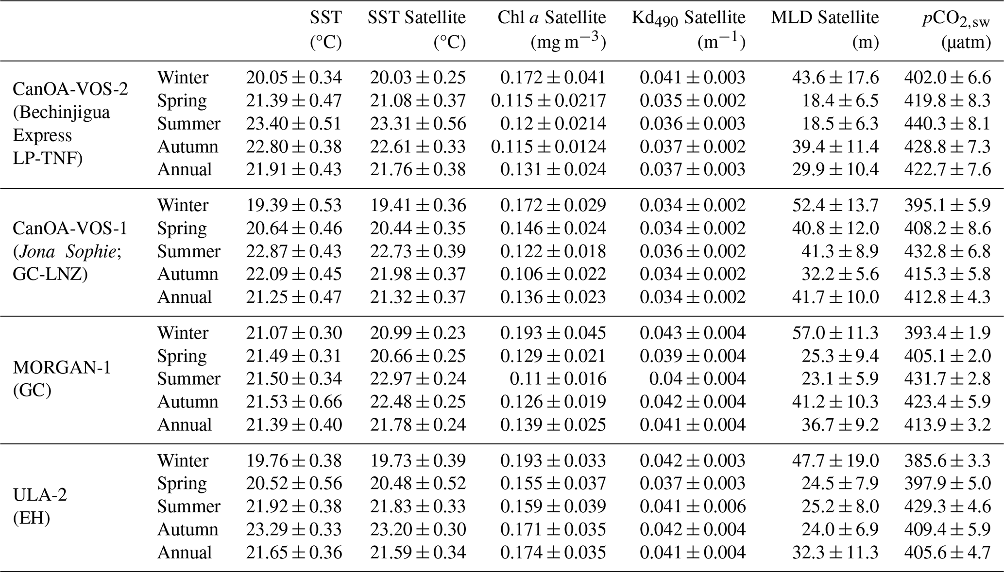
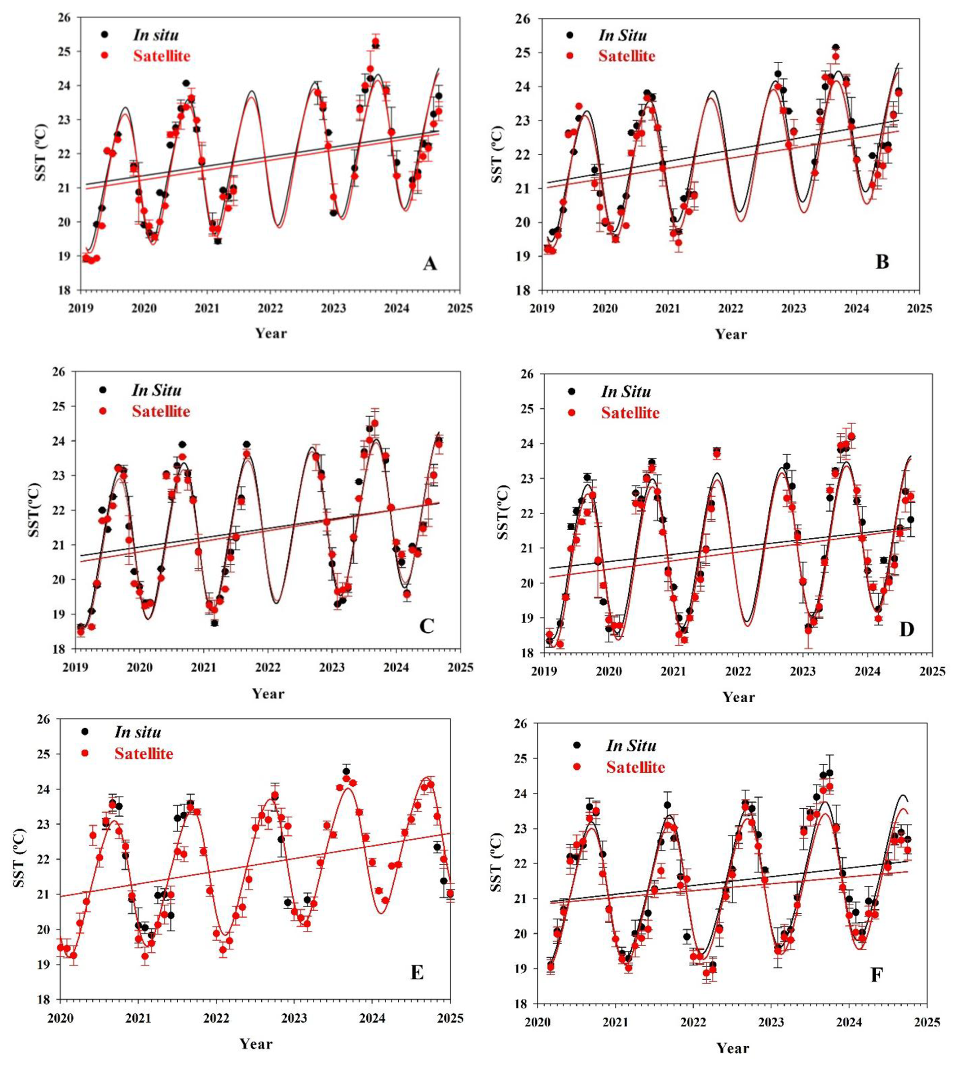
Figure 2 Monthly mean in situ SST (black) obtained from ship-based observations and moored buoys, and satellite-based SST (red) at locations (A)–(F). Harmonic fittings (Eq. 4) of the data are shown together with the linear fitting for the seasonally detrended data. Error bars represent the standard deviation of the measurements.

3.1 Variability of the SST data

Figure 2 shows the monthly mean SST derived from observations and satellite products at sites A–F. A clear seasonal cycle is evident across sites, with maximum SST in September (24.20 ± 0.76 °C in the western sites at A–B and 23.70 ± 0.68 °C in the eastern sites C–D) and minima in March (19.47 ± 0.24 and 18.97 ± 0.31 °C, respectively). Anomalous high SST were recorded during summer 2023, exceeding 25 °C at sites A–C and 24 °C at site D. The seasonal amplitude was 4.2 ± 0.4 °C along CanOA-VOS-1 and 4.5 ± 0.5 °C along the CanOA-VOS-2. Although no significant differences were found between sections within the same region (A vs B and C vs D), the mean SST at site D (20.59 ± 0.09 °C) was slightly lower than at site C (21.00 ± 0.09 °C). The covariance analysis between observational and satellite SST shows no significant differences between datasets (p<0.05). The mean daily residuals were 0.16 °C (SE = 0.12 °C) in the western region and 0.12 °C (SE = 0.10 °C) in the eastern region.

A seasonal SST cycle was evident at site E, despite the scarcity and temporal gaps of the ULA-2 buoy (Fig. 2E). Using the year with the most continuous data (2021), the seasonal amplitude was 5.10 ± 0.18 °C, with maximum SST in September (24.70 ± 0.26 °C) and minimum values in March (19.60 ± 0.40 °C). A comparable pattern was observed at site F from the MORGAN-1 buoy record (Fig. 2F), with SST peaking in September (23.71 ± 0.47 °C) and reaching its lowest in March (19.46 ± 0.52 °C), corresponding to a seasonal amplitude of 4.22 ± 0.51 °C.

Longitudinal variability in SST from both CanOA-VOS and satellite records is shown in Figs. 2 and S1 in the Supplement. In the western region, observed SST ranged from 20.59 ± 0.09 °C in winter to 24.04 ± 0.13 °C in summer, with an annual mean of 22.45 ± 0.11 °C. Seasonal averages matched those calculated from the satellite-derived data (0.1–0.2 °C), with the largest differences occurring in summer (0.26 °C). Although SST in the eastern region were lower throughout the year (annual mean 21.02 ± 0.27 °C), influenced by the Northwest African upwelling, similar seasonal variations were found (from 19.19 ± 0.24 °C in winter to 22.82 ± 0.25 °C in summer). Differences between in situ and satellite SST were smaller than those in the western region (0.05–0.2 °C). The west-east SST decrease persisted consistently along the longitudinally monitored span of the Canary archipelago, except for a slight warming associated with the island wake effect south of Tenerife captured along the CanOA-VOS-2 route (Fig. S1).

3.2 Predictive models of pCO_2,sw

Daily averaged pCO_2,sw and SST from all observational platforms, together with coincident satellite-derived chlorophyll a and MLD data at the same location, were used to train the four predictive models.

3.2.1 Multiple linear regression (MLR)

The first set of models used traditional multiple linear regression (MLR) to provide an initial, simple approximation of pCO_2,sw prediction. Five model configurations were tested, using different combinations of the available predictors: pCO_2,atm, SST, Chl a, Kd₄₉₀ and MLD, following the analytical form in Eq. (5). Considering the strong correlation between Chl a and Kd₄₉₀ (R²=0.96), Kd₄₉₀ was deemed non-significant and excluded from further analysis. The coefficients obtained for each configuration are listed in Table 2.

Table 2 Regression coefficients obtained from the multiple linear regression models for pCO_2,sw (top) and pH_T,is (bottom), applied to the different predictor combinations according to Eq. (5), using the full dataset.

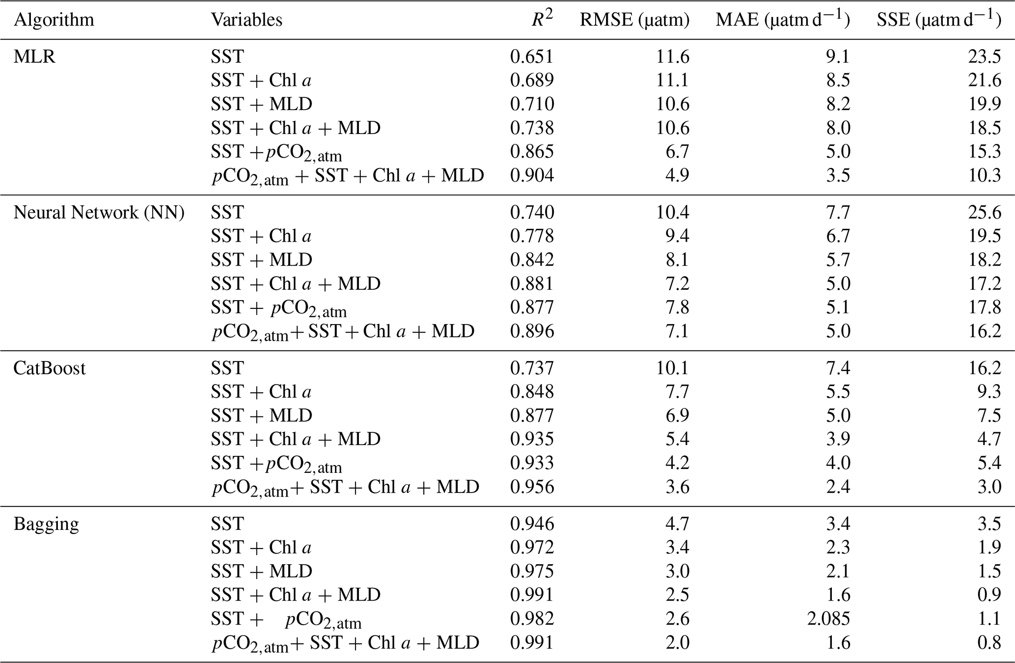
Model selection based on the Akaike Information Criterion (AIC_c<2) together with performance statistics (Table 3) suggest that the best-performing MLR included the atmospheric CO₂, thermal, physical and biological drivers (pCO${}_{\mathrm{2},\mathrm{atm}}+$ SST + MLD + Chl a). However, a two-variable model (SST and pCO_2,atm) produced comparable accuracy. Figure S2 shows measured versus predicted values for the training and validation datasets using four variables, pCO${}_{\mathrm{2},\mathrm{atm}}+$ SST + MLD + Chl a. Although many measured and predicted pCO_2,sw showed small differences, considerable scatter was observed, reflected in the performance metrics (Table 3). Validation results (Table S2) were consistent with training performance.

Table 3 Performance metrics for the comparison between predicted and measured pCO_2,sw (µatm) for each model using the training dataset.

3.2.2 Machine learning techniques

Table 3 compares the performance of the machine-learning approaches trained using observational pCO_2,sw data. All models were developed using the same dataset and input variables.

Neural Network (NN)

The first machine-learning method applied to predict pCO_2,sw was a neural network (NN). The performance metrics are presented in Table 3.

No analytical expression is provided, as the learned relationships are embedded within the synoptic weights of its neurons. Statistics indicate similar performances between the three-variable models (SST + MLD + Chl a) and the four-variable model, including pCO_2,atm, where two-variable models performed only slightly less effectively. Scatter plots of measured versus predicted pCO_2,sw for both training and validation datasets using the best NN model are shown in Fig. S2. Overall agreement was good, although prediction dispersion increased at higher pCO_2,sw, suggesting slightly poorer fitness in this range. For the training dataset, RMSE, MAE, SSE, and R² were 7.1 µatm, 5.0 µatm d⁻¹, 16.2 µatm² d⁻¹, and 0.891, respectively.

Categorical boosting (CatBoost) regression

The second machine-learning method applied to predict the pCO_2,sw in the Canary Archipelago was CatBoost. A total of 500 iterations were used to generate the prediction model. The performance statistics for all model configurations are summarised in Table 3. The pCO${}_{\mathrm{2},\mathrm{atm}}+$ SST + Chl a + MLD configuration yielded the best results, achieving the lowest RMSE, MAE and SSE, and the highest R². The performance of this model (Fig. S2), applied to both the training and validation datasets, yielded an R² greater than 0.95 with an RSME of only 3.6 µatm. The training dataset provided the most accurate results, with an MAE of 2.4 µatm d⁻¹ and an SSE of 3.0 µatm² d⁻¹. The validation statistics were consistent with those obtained during the training phase (Table S2).

Bootstrap aggregating (bagging) regression

A bagging algorithm was applied to predict pCO_2,sw using 200 bootstrap replicates. The computed statistics for the training set, combining the different parameters controlling the pCO_2,sw are summarised in Table 3.

Based on the statistical analysis, the models with the best predictive capacity were those that considered three or four parameters, as they yielded lower RMSE, MAE, and SSE. As observed in the previously fitted models, those including SST + MLD or SST +pCO_2,atm also performed well (Table 3). The bagging algorithm provided the highest R², lowest RMSE, MAE and SSE (0.991, 2.0, 1.6, 0.8, respectively) for any combination of variables, even when only SST was considered. The plot of measured versus predicted pCO_2,sw for both the training and validation sets using a four-variable model is shown in Fig. S2. This model presented low RMSE, MAE, and SSE (2.0 µatm, 1.6 µatm d⁻¹, and 0.8 µatm² d⁻¹, respectively). In this scenario, the application of the model to the validation set showed greater data dispersion than the training set (Table S2), due to the smaller sample size (Fig. S2).

3.3 Predictive models for pH_T,is

pH_T,is predictions were generated from the computed pH_T(A_T(SSS), fCO₂), using observations and satellite data (interpolated to the time and location of each observation) as input variables. In this case, pCO_2,atm was excluded from the predictive variables to avoid redundancy. Table 4 shows a comparison of the models employed in the machine-learning-based approaches. It is important to note that all models were developed using the same dataset and input variable.

Table 4 Performance metrics for the comparison between predicted and measured pH_T,is for each model using the training dataset.

3.3.1 Multiple linear regression (MLR)

The coefficients obtained for each of the four combination models are shown in Table 2. The statistical performance of these models is presented in Table 4. As observed for the pCO_2,sw fitting, the model including SST + Chl a + MLD provided the best performance for pH_T,is, with an R² of 0.745 and an RMSE of 0.006. The plot of measured versus predicted pH_T,is for model training (Fig. S3) shows a distribution similar to that of the validation dataset. This indicates that the number of data points used for validation was not a limiting factor for the model.

3.3.2 Machine learning techniques

All three techniques yielded higher correlation coefficients than those obtained using MLR (Table 4). The performance of the NN was lower than that of CatBoost, while bagging showed the best performance across all models. The model including three variables (SST + Chl a + MLD) was the most accurate for predicting pH_T,is in all cases (Table 4), with an R² of up to 0.99 and an RMSE as low as 0.002 when applying the bagging technique. Every combination of satellite data, even when considering only the SST, resulted in an R² greater than 0.95 with bagging. For CatBoost, the three-variable model was required to achieve an R² above 0.93.

We compared the accuracy indicators for the training and validation datasets for the three-variable models (Tables 4 and S3, Fig. S3) within the pH_T,is range of this study (7.97–8.07). When applying machine learning techniques, bagging consistently provided the best fit, ad increasing the data volume improved determination. RMSE, MAE, and SSE for both training and validation datasets remained below 0.01 in pH, reaching 0.002 and 0.003, respectively, when using bagging.

3.4 Validation of the results

The best prediction models for each class, based on the evaluated statistical parameters, were used to reconstruct the monthly mean pCO_2,sw and pH_T,is at sites A–D, and the results were compared. The temporal variability of observed and predicted values is presented in Fig. 3. All models successfully reproduced the seasonal cycle: pCO_2,sw reached its maximum in March and its minimum in August-September, while pH_T,is exhibited the opposite pattern. The predictions showed minor but statistically non-significant differences relative to the observations (p>0.05). No significant differences were detected among the linear, NN, CatBoost models (p<0.05). When comparing bagging predictions with observational data, no significant differences were found, confirming that boostrap aggregation yielded the most accurate representation of the measured values. Overall, observed pCO_2,sw were slightly higher than predicted ones, with mean differences of 1.7 ± 1.8 µatm for pCO_2,sw and 0.002 ± 0.001 for pH_T,is.

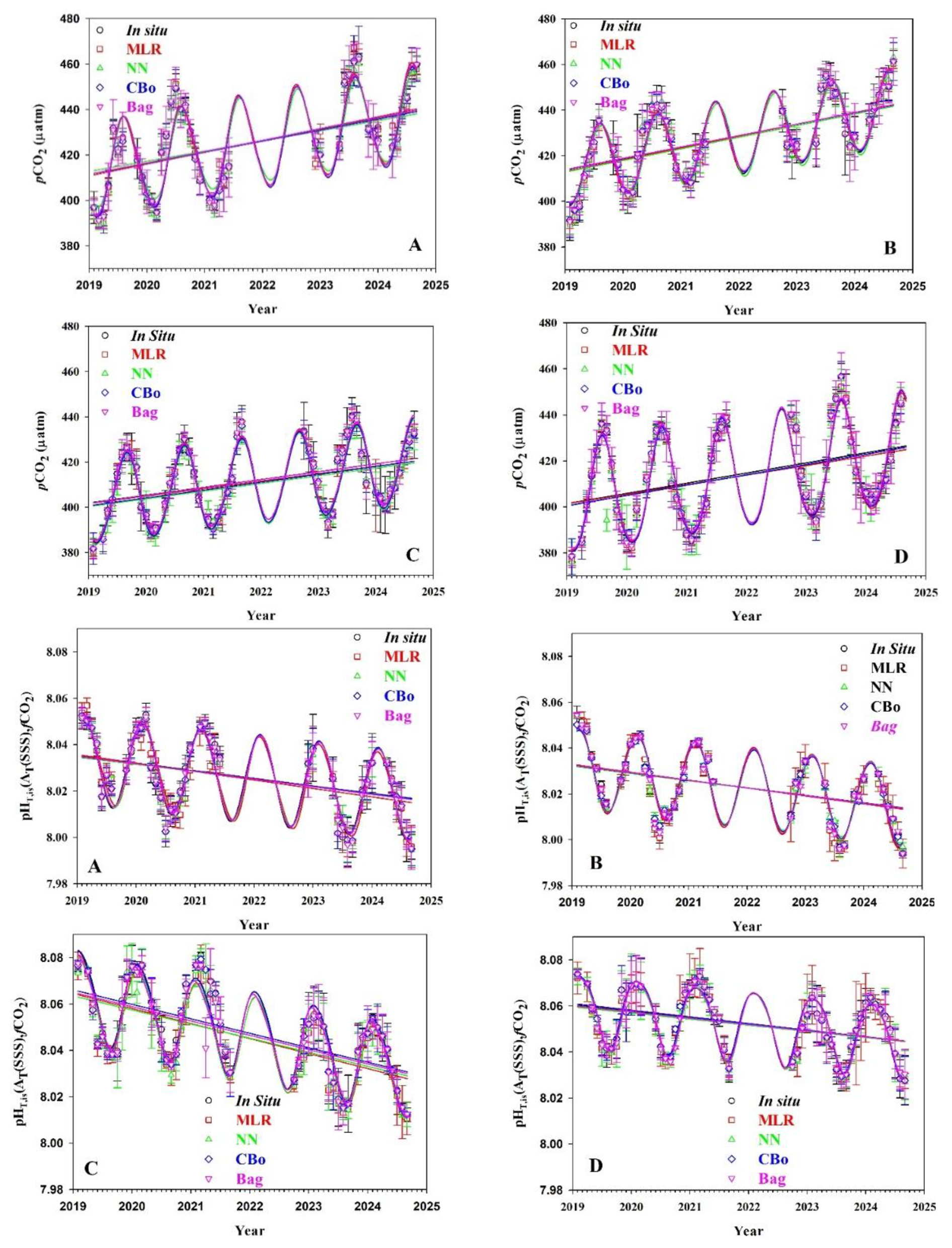
Figure 3 Monthly means of observational-based and model-predicted pCO_2,sw(pCO_2,atm, SST, Chl a, MLD) and pH_T(SST, Chl a, MLD) at the locations A–D (Fig. 1). MLR (red) means multilinear regression, NN (green) means neural network, CBo (blue) means CatBoost and Bag (purple) means bagging. Linear fittings for the seasonally detrended data are plotted.

Statistical differences (p>0.05) were detected when comparing the western and eastern sectors by ANCOVA. At sites A and B (Fig. 3), pCO_2,sw (and pH_T,is) varied seasonally between 404 ± 18 µatm (8.045 ± 0.012) and 449 ± 19 µatm (8.004 ± 0.010), with seasonal amplitudes of 47 ± 8 µatm (0.049 ± 0.005). At sites C and D (Fig. 3), seasonal values ranged between 390 ± 15 µatm (8.069 ± 0.008) and 440 ± 16 µatm (8.028 ± 0.012), with amplitudes of 52 ± 7 µatm (0.038 ± 0.006).

4 Discussion

Three oceanographic variables (SST, Chl a and MLD) with high-resolution satellite coverage for oceanic surface seawater, together with atmospheric CO₂ partial pressure, were used to model pCO_2,sw and pH_T,is in the Canary Archipelago. Salinity was excluded from the fitted models due to its negligible influence on pCO_2,sw variability (Sarmiento et al., 2007; Shadwick et al., 2010). Furthermore, satellite-derived salinity has been shown to differ considerably from in situ measurements, exhibiting elevated variability and uncertainty (Yu, 2020). Although Kd₄₉₀ was included in the initial model tests, its lack of statistical significance is likely due to its strong correlation with Chl a (R²=0.96), making it redundant and therefore not retained as a predictor.

4.1 The Canary Region during 2019–2024: Observational and modelling data

In the Canary Islands, the highest temperatures (Fig. 2) were recorded in late summer (September), driven by enhanced stratification of the water column and increased solar radiation. The lowest temperatures were measured in winter (February–March) due to convective mixing induced by surface cooling of the water column. This seasonal behaviour is consistent with the hydrographic conditions described at the ESTOC site, where surface waters exhibit a seasonal temperature amplitude of 4–6 °C, with minimum and maximum temperatures of 18 and 24 °C, respectively, recorded before 2023 (González-Dávila and Santana-Casiano, 2023). This range is also comparable to the SST observed in the easternmost region covered by the CanOA VOS-1 during 2019–2020 (Curbelo-Hernández et al., 2021).

The statistically significant differences (p<0.05) observed between the western and eastern sections are related to their distance from the African continent. The easternmost part of the archipelago is more exposed to upwelling filaments (Davenport et al., 1999), whereas the westernmost part is partially sheltered by the islands themselves. This spatial pattern, clearly visible in Figs. 2 and S1 as a progressive decrease in SST towards the African coast, is well captured by satellite observations. Their validation showed no significant differences (p<0.05), even near the islands. Therefore, satellite data were deemed suitable for model fitting and subsequent parameter estimation.

MORGAN-1 data (site F) show anomalously high SST during the summer of 2023, consistent with the occurrence of extreme SST conditions in the Canary Upwelling System in 2023 (Varela et al., 2024). Satellite data at the coastal buoy locations also showed anomalously high summer values, although these were on average 0.3 °C lower than those measured by the buoy sensors. In situ temperatures from June to October 2023 were more than 1 °C higher than those recorded in previous years. These elevated temperatures were not observed in 2024, indicating that 2023 should be considered an anomalous year in this region.

It is noteworthy that SST during February–March 2024 remained high. Winter SST (JFM) increased in 2024 and was, on average, 1 °C warmer than in the previous years (average for 2020–2022 was 19.09 ± 0.20 °C; average for 2023–2024 was 20.01 ± 0.25 °C). These anomalies strongly influence the trends observed in both satellite and observational datasets.

Harmonic fitting of temperature (Eq. 4) for the period March 2020 to March 2023, despite the limitation of only three years of data, indicates a warming trend of 0.03 °C yr⁻¹ in the seasonally detrended Gando Bay dataset (González et al., 2024). This rate is comparable to warming rates trends reported at the ESTOC site for the period October 1995 to March 2023 (González-Dávila and Santana-Casiano, 2023) and for the full Canary Upwelling System over 1982–2023 (Varela et al., 2024).

When considering the full five-year seasonally detrended in situ dataset from Gando Bay (March 2020 to October 2024), the warming rate increases to 0.19 ± 0.06 °C yr⁻¹ (0.14 ± 0.06 °C yr⁻¹ when derived from monthly mean satellite data). This SST increase was also observed at sites A–D (Fig. 2), where warming rates over the six years from February 2019 to October 2024 ranged from 0.29 ± 0.03 °C yr⁻¹ at sites A–C to 0.21 °C r⁻¹ at site D. The mean temperature at the western station (ULA-2) was ∼ 1 °C higher (22.12 ± 0.16 °C) than at the eastern station F (MORGAN-1; 21.13 ± 0.12 °C), reflecting the influence of Northwest African upwelling and island coastal upwelling. ANCOVA applied to both buoy datasets showed no significant differences between in situ and the satellite-derived SST, with mean differences below 0.19 °C, comparable to the regional mean difference of 0.15 °C for the full Canary dataset.

Satellite-derived data were used to predict pCO_2,sw and pH_T,is. The neural network model exhibited the highest prediction error (RMSE = 7.1 µatm, R²=0.896), whereas the MLR model performed slightly better (RMSE = 4.9 µatm, R²=0.904 for pCO_2,sw). Previous studies applying MLR along the US coasts reported RMSE values ranging from 22.4 to 36.9 µatm (Signorini et al., 2013), while NN-based approaches in the North and South Atlantic Ocean yielded RMSE values exceeding 19 µatm (Ford et al., 2022) and 21.68 µatm (Friedrich and Oschlies, 2009), respectively. In comparison, both MLR and NN models applied in the present study perform favourably, likely due to the limited spatial domain and the extensive observational dataset. For pH_T,is estimation, RMSE as low as 0.006 and 0.008 were obtained for MLR and NN, respectively, which fall within the typical analytical uncertainty.

The CatBoost empirical algorithm estimated pCO_2,sw and pH_T,is with uncertainties below 4 µatm and 0.004 pH, respectively, and R²>0.93 for both variables. This demonstrates robustness to uncertainty in satellite-derived variables influenced by different processes and coastal proximity, supporting its applicability in the region. However, the bagging approach exhibited exceptional performance, yielding uncertainties of 2.0 µatm for pCO_2,sw and 0.002 pH for pH_T,is over the period 2019–2024.

These particularly favourable results, and the comparatively low errors relative to ocean-scale models, likely arise because variability in pCO_2,sw and pH_T,is in the Canary Island waters is largely dominated by thermal effects (González-Dávila and Santana-Casiano, 2023; Takahashi et al., 2002). In this region, thermal control of surface carbonate chemistry is effectively captured by satellite-derived SST. In all cases, models using SST alone showed high correlation coefficients ($\mathrm{0.65}<R^{\mathrm{2}}<\mathrm{0.94}$). Although not the best-performing configurations, these single-variable models provide a reasonable representation of observed variability. The coefficient estimated from annual linear regression (10.40 µatm °C⁻¹, Table 2) deviates from the theoretical regional rate for 2019–2024 (16 µatm °C⁻¹; Takahashi et al., 2002), likely reflecting the influence of biological and physical processes (i.e., primary production, remineralisation and water mass mixing). Nevertheless, this rate remains consistent with those reported for ESTOC (Santana-Casiano et al., 2007).

Across all four sites and in Gando Bay, both observational data and model predictions indicate that pCO_2,sw increased between 2019 and 2024 at a rate of 3.8 ± 0.6 µatm yr⁻¹. The pH_T,is decreased at a rate of −0.004 ± 0.001 yr⁻¹ over the same period. Previous analyses at ESTOC for 1995–2023 (González-Dávila and Santana-Casiano, 2023) and at Gando Bay (site F) for 2020–2023 (González et al., 2024) reported a pCO_2,sw increase of 2.1 ± 0.1 µatm yr⁻¹ and a pH_T,is decrease of −0.002 ± 0.001 yr⁻¹. Comparable rates are observed across all selected sites when restricting analysis to March 2019–March 2023, excluding the anomalous conditions observed in late 2023, consistent with González et al. (2024).

4.2 Monthly pCO_2,sw and pH_T,is gridded maps

The bagging technique was used to construct gridded monthly maps of pCO_2,sw and pH_T,is for the Canary region (13–19° W, 27–30° N) over the study period. Results for the year 2023 are presented in Fig. 4. Monthly experimental averages are shown alongside the model predictions to illustrate the accuracy of the estimates. The expected seasonal pattern was reproduced, with higher pCO_2,sw in September and lower in March, and the opposite behaviour for pH_T,is. A clear longitudinal gradient was observed, with higher pCO_2,sw and lower pH_T,is toward the eastern sector, primarily driven by the thermal effect. Cooler seawater in the east, together with the influence of nutrient-rich, lower-pH Northeast African upwelled seawater (Pelegrí et al., 2005), counteract each other, increasing mean values while reducing seasonal amplitude.

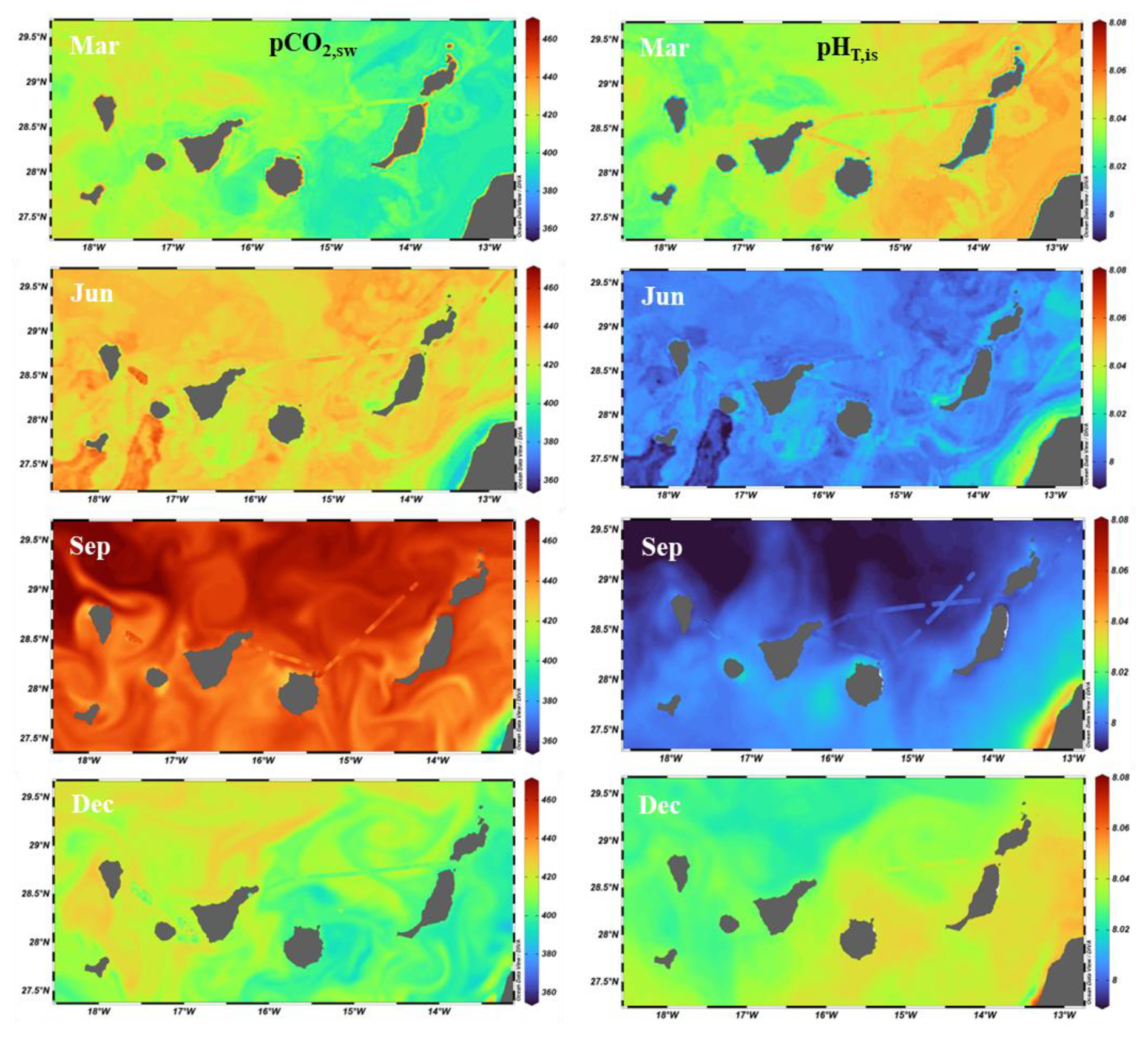
Figure 4 Gridded maps for pCO_2,sw (left) and pH_T,sw (right) predicted with bagging for the full March (Mar), June (Jun), September (Sep) and December (Dec) 2023 using pCO_2,atm and satellite conditions of SST, Chl a, and MLD together with observational data available for that month (the same colour code was used). Figure produced with Ocean Data View (Schlitzer, 2021; https://odv.awi.de, last access: 10 July 2025).

Several oceanographic features are apparent. Upwelling filaments, characterised by lower temperatures, locally reduce pCO_2,sw. In contrast, leeward island wake zones exhibit warmer waters, leading to increased pCO_2,sw and decreased pH_T,is. The African coastal upwelling signal is particularly evident in June and September, when lower pCO_2,sw and higher pH_T,is are observed as a result of enhanced biological activity that partially offsets the CO₂-rich upwelled waters.

Monthly mean pCO_2,sw and pH_T,is for the Canary Basin, predicted using the bagging approach for the period 2019–2024, are shown in Fig. 5. Monthly means were computed by applying the bagging model to daily satellite-derived SST, Chl a, and MLD, together with pCO_2,atm, and subsequently averaging the results spatially and temporally. Over these six years, mean pCO_2,sw was 419.7 ± 16 µatm, with a seasonal amplitude of 55 µatm. Harmonic fitting (Eq. 4) of the predicted time series indicates an increasing trend of 3.51 ± 0.31 µatm yr⁻¹ for 2019–2024, exceeding the contemporaneous increase in pCO_2,atm (2.3 µatm yr⁻¹).

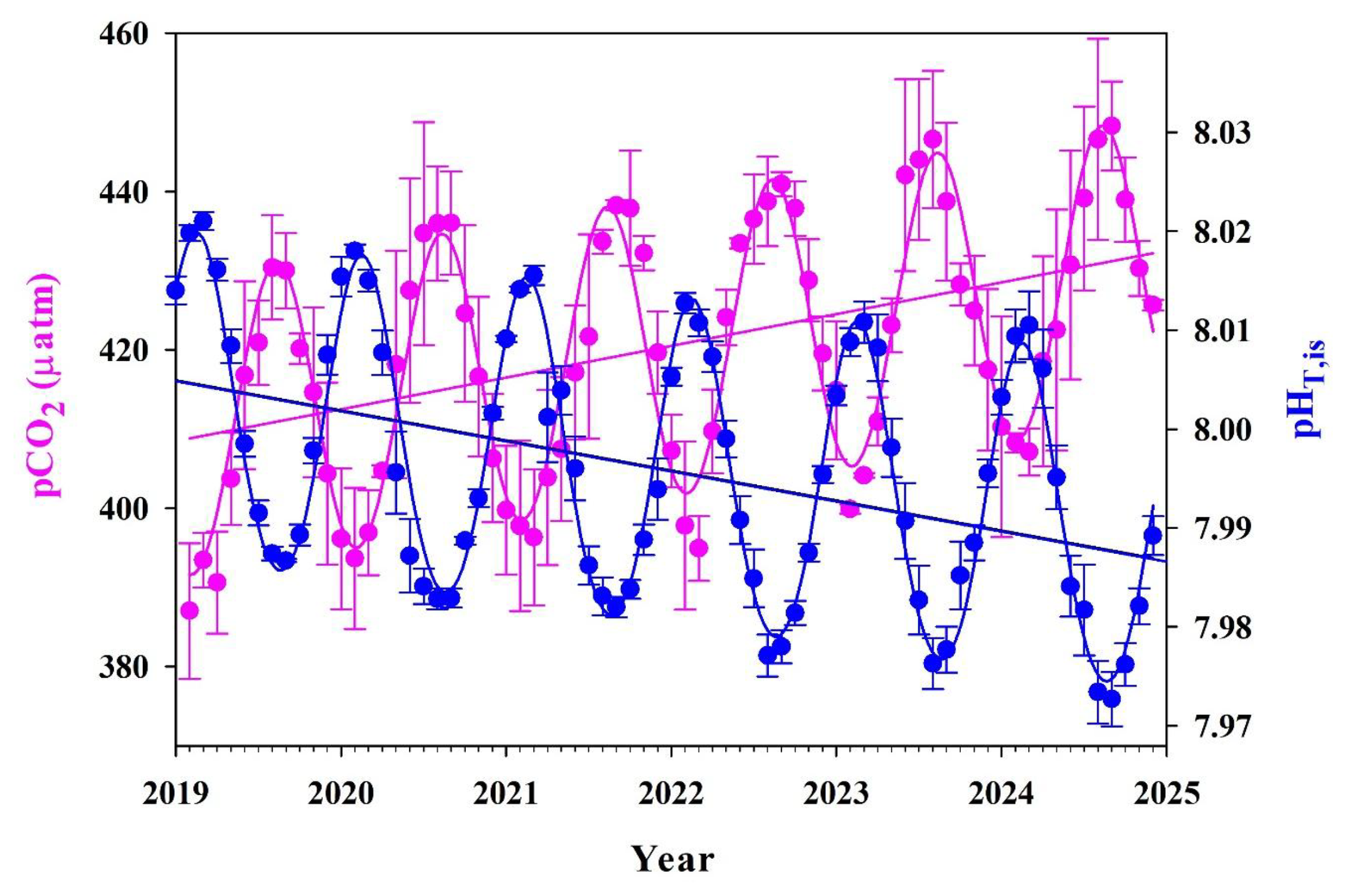
Figure 5 Monthly means of pCO_2,sw (µatm) and pH_T,sw predicted with bagging for 2019–2024 for the entire Canary region (27–30° N, 13–19° W). Linear fittings for the seasonally detrended data are also plotted.

Predicted pH_T,is (Fig. 5) ranged from 8.015 ± 0.049 in February–March to 7.980 ± 0.058 in September–October, reflecting a seasonal decrease of ∼ 0.04 pH from winter to summer. Elevated winter values reflect lower temperatures and enhanced convective mixing, whereas lower summer values are attributed to biological activity and water-column stratification (Santana-Casiano et al., 2001, 2007). This seasonal pH decrease is partially offset by the thermal effect, which compensates for approximately 33 % of the total decline. The thermal contribution corresponds to a pH decrease of 0.06 associated with a temperature increase of 4.1 °C. This compensating effect is evident near the African coast (Fig. 5), where upwelling of deep, cold, CO₂-rich waters reduces both SST and pH, generating a pronounced longitudinal gradient across the Canary region.

Figure 5 further shows that pH_T,is declined throughout the study period due to increasing ocean acidity, with a rate of −0.003 ± 0.001 yr⁻¹ derived from seasonally detrended data. The strong influence of MHW events, particularly during summer 2023 and winter 2023–2024, on the interannual trends of both variables is evident. The rise in pCO_2,atm is accompanied by an increase in SST of 0.2 °C yr⁻¹ over the six years, equivalent to a cumulative warming of 1.2 °C between 2019 and 2024. This increase is largely driven by the anomalously warm conditions in 2023, higher SST in winter 2020 compared to 2019, and elevated winter SST in 2023 and 2024 relative to 2022, when winter temperatures dropped below 18 °C and have since remained near 19 °C. These conditions have contributed to higher recent trends in pCO_2,sw and ocean acidification relative to long-term estimates at ESTOC, which were 2.1 µatm yr⁻¹ and −0.002 yr⁻¹, respectively, for the period 1995 to early 2023 (González-Dávila and Santana-Casiano, 2023). The limited six-year time series may also contribute to the magnitude of the observed rates. Notably, winters with SST exceeding 19 °C and summers with SST above 25 °C had not been recorded at the ESTOC site before 2023.

4.3 Long-term model prediction at ESTOC site

The bagging predictive model developed using data from the period 2019–2024 was applied to the ESTOC site for the period 2004–2024. Earlier years were not considered because the monthly satellite data before this period had lower spatial resolution. Satellite-derived SST, Chl a, and MLD, together with atmospheric pCO₂ computed from xCO₂ measurements at the Izaña (IZO) station, were used as model inputs (https://gml.noaa.gov/aftp/data/trace_gases/co2/flask/surface/txt/co2_izo_surface-flask_1_ccgg_event.txt, last access: 26 May 2025). Estimated values at 29°10^′ N and 15°30^′ W were compared with in situ observations from ESTOC (González-Dávila and Santana Casiano, 2023), updated to 2024, and are shown in Fig. 6. The model reproduced the ESTOC observations with mean residuals of 1.3 ± 3.1 µatm and yielded consistent trends of 1.9 ± 0.1 µatm yr⁻¹ over the study period, as determined from both model output and the seasonally detrended observational data.

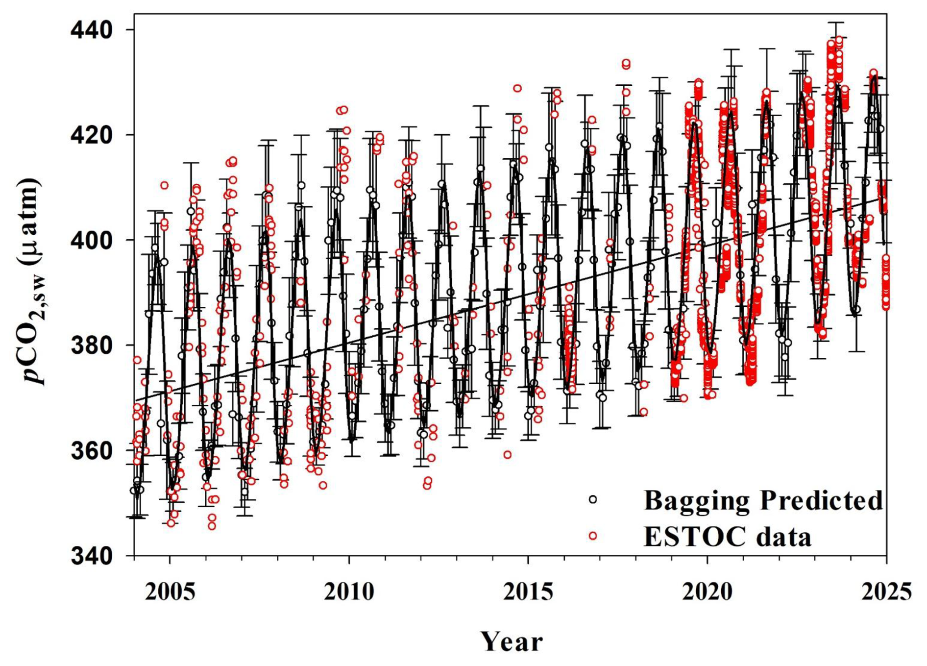
Figure 6 Monthly means of pCO_2,sw (µatm) predicted with bagging considering pCO_2,atm, SST, Chl a, MLD for the period 2004–2024 at the location of the ESTOC site (G in Fig. 1) and measured ESTOC pCO_2,sw.

When models excluding pCO_2,atm were applied, residuals increased to values exceeding 2 µatm, particularly during the early part of the record (2004–2010), when residuals approached 4 µatm. This behaviour reflects the increased weighting assigned to SST in the absence of atmospheric forcing, especially during periods characterised by strong thermal anomalies such as the 2023 marine heatwave in the Canary Upwelling System. Analysis of satellite-derived SST at the ESTOC site for 2004–2024 shows minimal temperature variability during 2004–2019 (0.0012 ± 0.002 °C yr⁻¹), followed by a marked warming trend during 2019–2024 (0.21 ± 0.01 °C yr⁻¹), consistent with the behaviour observed at sites A–F (Fig. 1). Consequently, when models based solely on SST, Chl a and MLD were applied to earlier periods, lower pCO_2,sw trends were predicted. In contrast, inclusion of pCO_2,atm in the model allows both thermal and atmospheric contributions to pCO_2,sw to be accounted for, ensuring that periods with weak SST trends still reflect the concurrent rise in atmospheric CO₂ and its influence on surface seawater pCO₂.

4.4 Air-sea CO₂ exchange in the Canary Archipelago

The predicted pCO_2,sw is highly useful for estimating FCO₂ with improved spatial and temporal resolution. Figure 7 shows FCO₂ calculated using the parametrisation proposed by Wanninkhof (2014) under monthly mean conditions for the period 2019–2024. The seasonal cycle of FCO₂ is primarily controlled by the large seasonal variability in pCO_2,sw, which governs ΔpCO₂, as pCO_2,atm exhibits a much smaller seasonal amplitude. In contrast, the effect of wind speed and gas solubility exhibits a smaller seasonal amplitude (Landschützer et al., 2014).

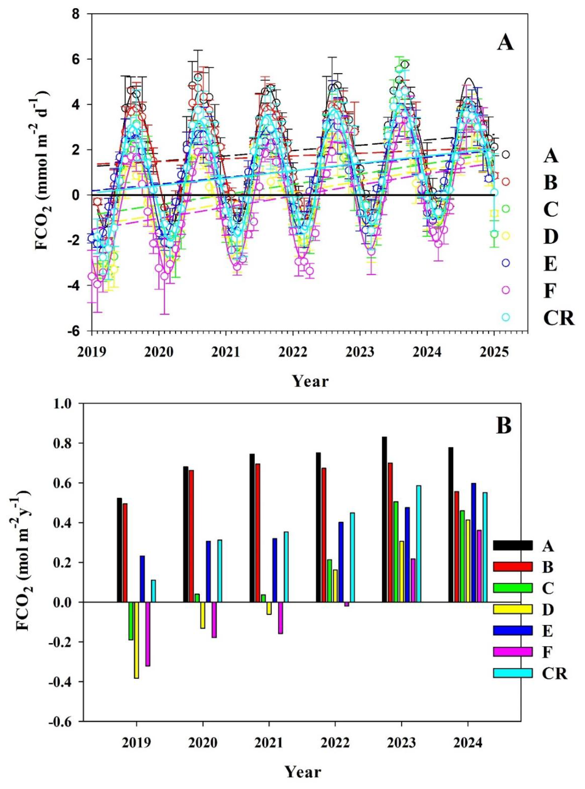
Figure 7 (A) Monthly means of FCO₂ (mmol m⁻² d⁻¹) in the Canary archipelagic waters predicted with bagging from 2019 to 2024 and (B) net annual FCO₂ (mol m⁻² yr⁻¹). In both plots, FCO₂ was represented at locations A–F and for the entire Canary Region (CR). Linear fittings for the seasonally detrended data are also plotted.

The region acts as a strong CO₂ sink during winter and spring, whereas during the warm season it behaves as a source. During the warm period from late May to early September (González-Dávila et al., 2003), when the dominant trade winds impact the Canary Islands, pCO_2,sw exceeds pCO_2,atm. This leads to higher wind speeds and reinforces the role of CO₂ supersaturation in the total flux estimation, favouring the region's role as a CO₂ source.

Sites located closer to the African continent (C and D) and the coastal waters (F in the Gando Bay, also in the eastern part of the Canary Islands) are more likely to act as a CO₂ sink than the westernmost region (Curbelo-Hernández et al., 2021). This behaviour is primarily associated with the thermal gradient, with temperatures more than 1 °C lower than in the western sector, as well as with higher biological productivity. However, Fig. 7B shows that, due to the increase in SST across the Canary Islands during the study period, all locations that previously acted as an annual CO₂ sink shifted to behaving as a source after 2022.

For the period 2019–2024, the Canary region acted as a weak CO₂ source, with a mean flux of 0.39 ± 0.17 mol m⁻² yr⁻¹. Increasing flux trends were observed across all sub-regions, ranging from 0.18 to 0.37 mmol m⁻² d⁻¹, with an average rate of 0.25 ± 0.02 mmol m⁻² d⁻¹. When considering the entire Canary region (13–19° W, 27–30° N), covering an area of 185 000 km² after excluding the island land masses, the system transitioned from a weak source of 0.9 Tg CO² in 2019 to a source of 4.5 Tg CO₂ in 2024, with a maximum of 4.8 Tg CO₂ in 2023. This peak coincided with the highest SST recorded during the study period (Fig. 2), favouring the largest increase in pCO_2,sw.

These estimates are primarily based on surface water measurements, particularly those derived from satellite data. Although such datasets provide high spatial resolution and robust representation of surface trends, they do not capture subsurface processes or vertical gradients in CO₂ and temperature.

5 Conclusions

This study presents the first predictive modelling framework for surface seawater pCO_2,sw and pH_T,is in the Canary Islands basin. The results demonstrate the value of satellite observations as a complement to in situ platforms such as voluntary observing ships and moored buoys. By combining satellite products from the Copernicus Marine Environmental Monitoring Service with in situ observations, it was possible to characterise the variability of pCO_2,sw and pH_T,is in the waters surrounding the Canary Islands and to quantify the regional air-sea CO₂ flux.

Four modelling approaches, ranging from classical multivariate statistics to more sophisticated machine-learning techniques, were applied using atmospheric pCO₂, SST, Chl a, and MLD as controlling variables. Multiple linear regression, neural network, and categorical boosting models yielded comparable results, with RMSE, MAE, and R² values similar to those reported for oceanic-scale applications. Among all approaches, the bagging model provided the best performance, with RMSE values below 2.5 µatm (< 0.7 %) for pCO_2,sw and 0.002 for pH_T,is, R² exceeding 0.99, and no significant differences relative to monthly mean observations.

Application of the bagging approach enabled a detailed description of the seasonal and longitudinal variability of pCO_2,sw and pH_T,is across the Canary region. After confirming agreement between in situ and satellite-derived SST within ±0.15 °C, the model was trained using measured xCO_2,sw (converted to pCO_2,sw) together with satellite SST, chlorophyll a and MLD, providing high-resolution spatial and temporal coverage. A persistent longitudinal SST gradient of ∼ 1 °C, driven by African coastal upwelling and offshore transport of upwelling filaments, resulted in systematically higher pCO_2,sw and lower pH_T,is values in the western sector (between El Hierro and Tenerife) compared with the eastern sector (between Tenerife and Lanzarote). In terms of air-sea CO₂ exchange, the western region acted as a source throughout the study period, whereas the eastern region transitioned from a weak sink to a source after 2022. The increasing trend in SST across the Canary region, particularly during the anomalous warm year 2023 and during warmer winters in 2020, 2023 and 2024, is identified as the main driver of enhanced CO₂ outgassing. Overall, the Canary region acted as a net CO₂ source of 0.39 ± 0.17 mol m⁻² yr⁻¹ between 2019 and 2024, increasing from 0.9 Tg CO₂ in 2019 to 4.5 Tg CO₂ in 2024, with a maximum of 4.8 Tg CO₂ in 2023. These results highlight the complexity of modelling pCO_2,sw and pH_T,is in coastal and island-influenced environments, where physical and biological is greater than in the open ocean. The pronounced influence of the 2023 marine heatwave, which persisted for more than one year, underscores the sensitivity of short time series to extreme events and reinforces the need for long-term observations when assessing interannual trends. Although model performance is robust, longer time series are required to better constrain long-term changes in pCO_2,sw and pH_T,is in the Canary Islands waters. Nevertheless, this study demonstrates that the integration of sustained observations, satellite data and machine-learning techniques provides a powerful framework for characterising regional air-sea CO₂ exchange.