Externally-forced and intrinsic variability of the Mediterranean surface and overturning circulations

Part of Mediterranean Sea variability is forced and paced by external drivers (e.g. atmosphere, river runoffs, Atlantic inflow), while the other part has a random phase and spontaneously emerges due to chaotic intrinsic variability (CIV). This study quantifies across time scales the imprints of both variability components on the surface and zonal overturning circulations within the basin, from a 39-year 30-member ensemble ocean $\mathrm{1}/\mathrm{12}$° simulation. We find that most of sea surface height (SSH) variance is intrinsic over 17 % of the basin, in particular in the southern Ionian and Levantine basins, and most notably in the Algerian basin where CIV explains 80 % of the SSH variance at periods greater than 4 months. In contrast, 75 % of the interannual-to-decadal SSH variance of the North Ionian Gyre circulation is paced by the atmosphere, suggesting an external triggering of the Adriatic-Ionian Bimodal Oscillating System (BiOS) reversal. CIV exerts a larger influence on the Rhodes, Bonifacio, and Alboran gyre circulations. Fluctuations of the density-coordinate zonal overturning circulation (ZOC_σ) and of associated transports are mostly paced by the forcing over the basin. However, CIV tends to explain a larger fraction of these transports variance in the intermediate and bottom layers near deep convection sites, in particular in the Levantine basin where this fraction exceeds 50 % between 27 and 30° E at submonthly periods, 30 % at subannual periods, and 20 % at longer periods (reaching 20 years locally). This partly random character of the multi-scale Mediterranean variability has implications for evaluating model simulations and designing long-term observation systems, which are finally discussed.

1 Introduction

The large-scale circulation of the Mediterranean Sea may be sketched as a zonal overturning, whose shallow limb is fed by the eastward surface inflow of Atlantic Waters entering through the Strait of Gibraltar. These waters become progressively denser as they flow eastward and finally contribute to the formation of Levantine Intermediate Water (LIW), which feeds a westward return flow at intermediate depth. A counterclockwise cell sits below; deep waters mostly formed by wintertime convection in the Gulf of Lions, the Adriatic Sea, and the Aegean Sea sink and partly feed the lower cell and the westward intermediate flow, which then exits the basin within the Gibraltar overflow (Demirov and Pinardi, 2007; Pinardi et al., 2015, 2019).

An overall cyclonic circulation to the north of the basin, and a number of persistent horizontal circulation features such as the Alboran Gyres, the Algerian eddies, the North Ionian Gyre (NIG), are superimposed on this meridionally-integrated overturning upper cell (Millot and Taupier-Letage, 2005; Schroeder et al., 2012). Alongside active mesoscale eddies and other modes of multi-scale variability, these multiple circulation features are influenced by the basin’s complex geometry and drive fluctuating three-dimensional transport and redistribution of water properties and mass in three dimensions across the basin (Millot et al., 1990; Robinson et al., 2001; Viúdez et al., 1998; Gačić et al., 2010; Menna et al., 2019).

This time-varying circulation is forced at first order by external drivers, such as the exchanges with the Atlantic Ocean through the Strait of Gibraltar, the atmospheric forcing, and river runoffs (Pinardi and Masetti, 2000; Demirov and Pinardi, 2007). However, recent studies have shown that a substantial part of the ocean variability may arise spontaneously, i.e. from intrinsic fluctuations generated by ocean nonlinearities. Beyond its oceanic origin, this variability also has a random phase and is thus often labeled “chaotic intrinsic variability” (see e.g. Bessières et al., 2017; Wolfe et al., 2017). This phenomenon therefore acts as a source of uncertainty in oceanic hindcasts and forecasts, and question the attribution of oceanic fluctuations to external drivers solely. Rubino et al. (2023) and Gnesotto et al. (2024) have shown from idealized eddying simulations of the basin that mesoscale–topography interactions alone can generate intrinsic variability up to decadal scales, even without variable forcing. Using observations, idealized simulations, or laboratory experiments, Gačić et al. (2010), Civitarese et al. (2023), and Rubino et al. (2020) have suggested that interannual-to-decadal reversals of the NIG may also be driven by CIV operating within the Adriatic–Ionian Bimodal Oscillating System (BiOS); the sole oceanic origin of such reversals is still debated though, as other authors highlight the impact of large-scale wind stress curl anomalies on the NIG reversals (Pinardi and Masetti, 2000; Demirov and Pinardi, 2002; Nagy et al., 2019; Liu et al., 2022). Realistic ocean model studies help investigate in more complex contexts how intrinsic mechanisms compete with external drivers in generating variability. Such studies have suggested in particular that a significant fraction of the basin-scale seasonal sea surface height (SSH) variability is intrinsic (Benincasa et al., 2024), that deep convection in the Gulf of Lions is modulated by a strong sub- to inter-annual intrinsic variability (Waldman et al., 2017, 2018). Most realistic model studies, however, were focused on specific regions or relatively short timescales, leaving the impacts of intrinsic variability and of the external forcing partly unexplored at interannual-to-decadal timescales over the whole basin.

The OceaniC Chaos – ImPacts, strUcture, predicTability (OCCIPUT) project has shown from an ensemble of $\mathrm{1}/\mathrm{4}$° global ocean/sea-ice simulations (Bessières et al., 2017; Penduff et al., 2014) that the contribution of CIV may indeed compete with, and locally dominate the (externally-) forced variability of several oceanic indices in many regions of the global ocean, up to the scale of basin gyres and multiple decades. For instance, Leroux et al. (2018) and Carret et al. (2021) emphasized the substantial imprint of CIV on the subannual-to-decadal Atlantic overturning circulation and on regional SSH fields, respectively. However, the relatively modest OCCIPUT model resolution limits its ability to represent fine-scale Mediterranean dynamics, especially mesoscale–topography interactions that are likely important for the generation of intrinsic variability in this basin.

The goal of the present study is to evaluate the imprints of (atmospherically-)forced and intrinsic ocean variability over the Mediterranean Sea, with an emphasis on interannual and longer scales. We use a relatively large (30 members) and high resolution ($\mathrm{1}/\mathrm{12}$°, 7–8 km) realistic ensemble simulation spanning almost 4 decades to disentangle the external and intrinsic sources of Mediterranean variability, aside from the seasonal timescales on which Benincasa et al. (2024) focused. Compared with OCCIPUT, this $\mathrm{1}/\mathrm{12}$° configuration is expected to provide a more realistic representation of mesoscale activity, boundary current instabilities, and dense water formation processes in the Mediterranean Sea.

We focus on the variability of three complementary indices derived from the simulation and from observations when available: (i) SSH, which captures the imprint of mesoscale and horizontal circulation; (ii) SSH-derived relative vorticity of various gyres (including the NIG) and recirculation features; and (iii) components of the zonal overturning circulation (ZOC) computed in density space, which link the surface, intermediate and bottom branches of the Mediterranean large-scale circulation.

The remainder of the paper is organized as follows. Section 2 describes the ensemble simulation, the observational products, and our post-processing techniques. Section 3 provides an assessment of the model skill with respect to observational products and existing studies from subannual to decadal timescales. Section 4 then assesses the contributions of external and intrinsic sources of this multi-scale variability. Section 5 summarizes the main conclusions and discusses the broader implications of these findings.

2 Datasets and methods

2.1 Ensemble ocean simulation

Our ensemble ocean simulation is based on the NEMOMED12 configuration of the NEMO ocean model, implemented over the Mediterranean basin at 1/12^∘ resolution and over 75 vertical levels, and driven by specified forcing between 1979 and 2017. Beuvier et al. (2012), Adloff et al. (2015), Hamon et al. (2016), and Waldman et al. (2017) have presented this model configuration in detail, and evaluated its skill in representing the circulation and water masses of the basin, when driven by earlier versions of our atmospheric forcing.

Our surface forcing is provided by the new ALDERA3 dataset, which consists in 3-hourly air-sea fluxes (wind stress, heat and freshwater fluxes). This dataset was developed by dynamically downscaling the ERA5 reanalysis at 12 km resolution with the version 6 of the CNRM-ALADIN regional climate model (Nabat et al., 2020) using a spectral nudging option (Colin et al., 2010) to increase the large-scale control of ALADIN by ERA5. With respect to the first version of ALDERA (Hamon et al., 2016), ALDERA3 was designed to improve the output temporal resolution, cover the more recent years thanks to the ERA5 forcing, improve the large-scale chronology via the spectral nudging technique, use a smoother interpolation of the sea surface temperature (SST) forcing, and add an explicit representation of natural and anthropogenic aerosols interacting with the radiative and cloud schemes (see Nabat et al., 2020). ALDERA3 covers the whole Med-CORDEX domain and is a contribution to this international initiative (Ruti et al., 2016). A Newtonian relaxation is applied to NEMOMED12 SSTs during the simulation to maintain thermal stability, with a restoring coefficient equivalent to 40 W m⁻² K⁻¹.

River runoff is prescribed at the river mouths and along the coastline as a surface freshwater flux. A 1980–2017 climatological seasonal cycle derived from the interannual dataset of Ludwig et al. (2009) is used. Major Mediterranean rivers fluxes are directly taken from the database, other smaller rivers are gathered into a coastal runoff (Hamon et al., 2016; Waldman et al., 2017). Boundary forcing in the Gulf of Cadiz is applied in each ensemble member within a buffer zone, where the model temperature, salinity and SSH fields are relaxed towards their monthly climatological counterparts extracted from the ORAS4 global ocean reanalysis (Balmaseda et al., 2013), with a relaxation time scale decreasing westwards. More details about the model configuration and the buffer zone are given in Beuvier et al. (2012) and Adloff et al. (2018).

The simulation starts with a 20-year one-member spin-up (1979–1998), which adjusts the upper part of the basin. The 30 ensemble members are then initialized by this spun-up state, and subsequently driven by the same surface and lateral fluxes throughout the 39-year integration period (from January 1979 to December 2017). Ensemble dispersion is generated by introducing slight stochastic perturbations to the biharmonic viscosity coefficient (perturbations amount to 0.01 % of the nominal coefficient) during the first 6 months of the run. These tiny perturbations are shut off on 27 June 1979 for the rest of the integration. The ensemble spread grows and stabilizes in amplitude after about 3 years (not shown).

We will thus focus our analyses over the period 1982–2017, over which all ensemble members share the same model setup, the same atmospheric and lateral forcing, ensuring that ensemble dispersion is solely due to intrinsic ocean variability emerging inside the domain. The use of climatological relaxation fields in the Gulf of Cadiz implies that non-seasonal Atlantic variability is absent from our simulation; in other words, the forced and intrinsic non-seasonal variabilities on which we shall focus are endemic to the Mediterranean basin.

2.2 Sea Surface Height observational product

The observational dataset used in this study is the European Seas Gridded Sea Surface Height product, distributed by the Copernicus Marine Service (CMEMS, 2026). This product provides daily sea level fields on a $\mathrm{1}/\mathrm{8}\mathit{°}\times \mathrm{1}/\mathrm{8}\mathit{°}$ grid over the European seas, covering the period from January 1993 to December 2017. It provides Absolute Dynamic Topography (ADT) derived by combining Sea Level Anomalies (SLA) with a Mean Dynamic Topography using the DUACS system (Data Unification and Altimeter Combination System). ADT is used as the observational counterpart to the model SSH, allowing direct comparison between modeled and observed daily sea level fields over the Mediterranean Sea, after subtraction of their spatial means.

2.3 Diagnostics

2.3.1 Geostrophic vorticity

The vertical component of geostrophic relative vorticity is derived from SSH as

$$\begin{array}{}\text{(1)}& \mathit{\zeta }={\displaystyle \frac{g}{f}}{\mathrm{\nabla }}^{\mathrm{2}}\mathrm{SSH}\end{array}$$

within each ensemble member and from the observational product, where g is the gravitational acceleration and f the Coriolis parameter. We computed vorticity from low-frequency SSH fields (see Sect. 2.3.3), and averaged the result over localized boxes shown in Fig. 1. The resulting timeseries characterize the slow evolution of regional gyre-like features of interest.

2.3.2 Overturning

The Mediterranean zonal overturning circulation provides a quantitative meridionally-integrated view of volume transports and water mass transformations within the basin, from their surface inflow to their subsurface outflow through Strait of Gibraltar (Sayol et al., 2023). In order to assess the imprint of forced and intrinsic variability on the zonal transports in various density classes throughout the basin, we computed in each ensemble member the zonal overturning circulation (ZOC_σ, in Sverdrups: 10⁶ m² s⁻¹) in density space from potential density referenced at the surface (σ₀) and velocity fields saved as successive 5-daily averages, as described in Hirschi et al. (2020):

$$\begin{array}{}\text{(2)}& \begin{array}{rl}{\mathrm{ZOC}}_{\mathit{\sigma }}(x,{\mathit{\sigma }}_{\mathrm{0}},t,n)& =\underset{y_{\mathrm{1}}}{\overset{y_{\mathrm{2}}}{\int }}\underset{-h(x,y)}{\overset{\mathit{\eta }}{\int }}u(x,y,z,t,n)\\ & \times H\left({\mathit{\sigma }}_{\mathrm{0}}\right(x,y,z,t,n)-{\mathit{\sigma }}_{\mathrm{0}})\mathrm{d}y\mathrm{d}z\end{array}\end{array}$$

where y₁ and y₂ denote the basin's latitudinal boundaries (5 and 45° N), η the free surface height, h(x,y) the bottom depth, σ₀ the reference isopycnal for transport integration, $u(x,y,z,t,n)$ the zonal velocity at depth z and time t in member n, and H the Heaviside step function with H(x)=1 for x>0 and H(x)=0 otherwise. Time series of zonal transports are finally derived from ZOC_σ as explained in Sect. 3.2, post-processed as explained in the next two sections, and analyzed in the rest of the paper.

2.3.3 Temporal scale decomposition

The 1979–2017 linear trends and mean seasonal cycles are removed from all SSH and ZOC-derived time series before decomposing them into temporal scales. Each of the resulting time series, noted X(x,t) at location x and time t, may be then decomposed following Sérazin et al. (2015):

$$\begin{array}{}\text{(3)}& X(\mathit{x},t)=\stackrel{\mathrm{‾}}{X}\left(\mathit{x}\right)+X_{\text{LF}}(\mathit{x},t)+X_{\text{HF}}(\mathit{x},t),\end{array}$$

where

• $\stackrel{\mathrm{‾}}{X}\left(\mathit{x}\right)$ is the temporal average;

• X_LF(x,t) is the low-frequency (LF) component (variability with periods longer than about 2.5 years) calculated by applying a low-pass Lanczos filter with a cut-off period of 912 d; the first and last 2 years of filtered time series are discarded to avoid filtering side effects.

• $X_{\text{HF}}(\mathit{x},t)=X(\mathit{x},t)-X_{\text{LF}}(\mathit{x},t)$ is the high-frequency (HF) component. Interannual variability is thus included in the HF component.

2.3.4 Total, intrinsic and forced variabilities; intrinsic variance ratios

All variance estimates presented below were computed from demeaned, detrended, deseasonalized time series within all members, with or without decomposition into temporal scales (see Sect. 2.3.3). Let X_n(t) be the time series of a variable of interest in the n-th ensemble member, with $t\in [\mathrm{1},T]$, $n\in [\mathrm{1},N]$, and N=30. Let overbars and brackets denote temporal and ensemble means, respectively: $\stackrel{\mathrm{‾}}{X_n}=\frac{\mathrm{1}}{T}{\sum }_{t=\mathrm{1}}^T{X}_n\left(t\right)$, and $\langle X\rangle \left(t\right)=\frac{\mathrm{1}}{N}{\sum }_{n=\mathrm{1}}^N{X}_n\left(t\right)$. These operators are used to split the total variability X_n(t) into its (externally-) forced and intrinsic components following Hogg et al. (2022).

• The forced variability component is common to all members, and is thus estimated as the time-varying ensemble mean: X_F(t)=〈X〉(t).

• The intrinsic variability component in member n is computed by subtracting the forced from the total variability: $X_{\mathrm{I},n}\left(t\right)=X_n\left(t\right)-X_{\mathrm{F}}\left(t\right)$. By construction, $\stackrel{\mathrm{‾}}{X_{\mathrm{I},n}}=\mathrm{0},\forall n$.

The variances of the total signal X_n, and of its forced (X_F) and intrinsic (X_I) components are estimated and compared as follows:

• Mean variance of the total variability: ${\mathit{\sigma }}_{\mathrm{T}}^{\mathrm{2}}=\langle \stackrel{\mathrm{‾}}{\left(X_n\right(t)-\stackrel{\mathrm{‾}}{X_n}{)}^{\mathrm{2}}}\rangle$

• Mean variance of the forced variability: ${\mathit{\sigma }}_{\mathrm{F}}^{\mathrm{2}}=\stackrel{\mathrm{‾}}{\left(X_{\mathrm{F}}\right(t)-\stackrel{\mathrm{‾}}{X_{\mathrm{F}}}{)}^{\mathrm{2}}}$

• Time dependent variance of the intrinsic variability (or instantaneous ensemble variance): ${\mathit{\sigma }}_{\mathrm{I}}^{\mathrm{2}}\left(t\right)=\langle X_{\mathrm{I},n}(t{)}^{\mathrm{2}}\rangle$

• Time dependent intrinsic variance ratio (or instantaneous contribution of intrinsic processes to the total variance): $R_{\mathrm{i}}\left(t\right)=\frac{{\mathit{\sigma }}_{\mathrm{I}}^{\mathrm{2}}\left(t\right)}{{\mathit{\sigma }}_{\mathrm{T}}^{\mathrm{2}}}$

• Mean variance of the intrinsic variability: ${\mathit{\sigma }}_{\mathrm{I}}^{\mathrm{2}}=\stackrel{\mathrm{‾}}{{\mathit{\sigma }}_{\mathrm{I}}^{\mathrm{2}}\left(t\right)}$

• Mean intrinsic variance ratio $R_{\mathrm{i}}=\stackrel{\mathrm{‾}}{R_{\mathrm{i}}\left(t\right)}$.

Our choice of biased variance estimates applied on zero-mean detrended time series ensures that ${\mathit{\sigma }}_{\mathrm{T}}^{\mathrm{2}}={\mathit{\sigma }}_{\mathrm{F}}^{\mathrm{2}}+{\mathit{\sigma }}_{\mathrm{I}}^{\mathrm{2}}$ (Narinc et al., 2024).

3 Assessment of the ensemble simulation

Before disentangling the forced and intrinsic components of variability from our simulation, we first assess how well the model driven by ALDERA3 reproduces the mean features and the total variability of the Mediterranean horizontal and overturning circulations, at both low- and high-frequency.

3.1 Sea Surface Height (SSH)

3.1.1 Time averaged SSH

At first order, the Mediterranean surface circulation is characterized by cyclonic and anticyclonic gyres and semi-permanent jets. These coherent structures persist throughout the simulation and are clearly visible in both the time-averaged altimetric observations and the time-ensemble-averaged model fields, shown in Fig. 1a–b.

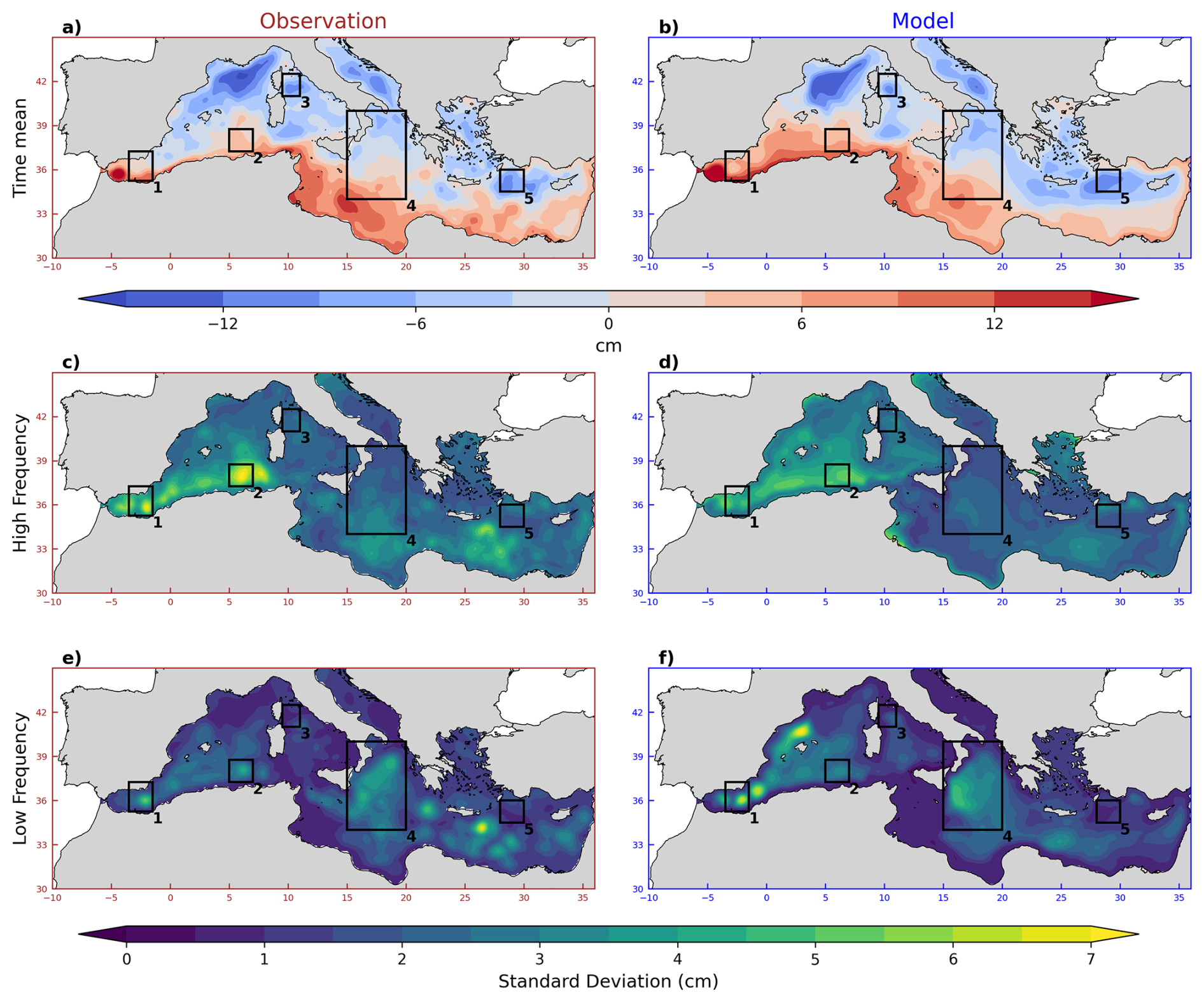
Figure 1 Time-averaged SSH between 1995 and 2015 from the Copernicus observational product (a) and from the ensemble-averaged simulation outputs (b). Total SSH standard deviation from satellite altimetry at high-frequency (c) and low-frequency (d). The same quantities derived from the simulation are shown respectively in (e) and (f). The black boxes surround the gyres investigated in Sect. 4.2: (1) Eastern Alboran Gyre, (2) Algerian Gyre, (3) Bonifacio Gyre, (4) North Ionian Gyre (NIG), and (5) Rhodes Gyre.

The model skillfully simulates the time-averaged general circulation in most parts of the basin, in particular large-scale features such as the inflow of Atlantic waters along the north African coast, the cyclonic gyres in the Gulf of Lions, in the Southern Adriatic Sea, and the Rhodes Gyre. The main simulation-observation difference appears in the Balearic sea (2° W to 1° E along the Spanish coast), where the observations reveal a weak cyclonic geostrophic circulation that has an opposite sign in the simulation. In the south and west of Crete, smaller circulation features – Ierapetra (35° N; 26° E) and Pelops (36° N; 22° E) gyres – appear less clearly in the model.

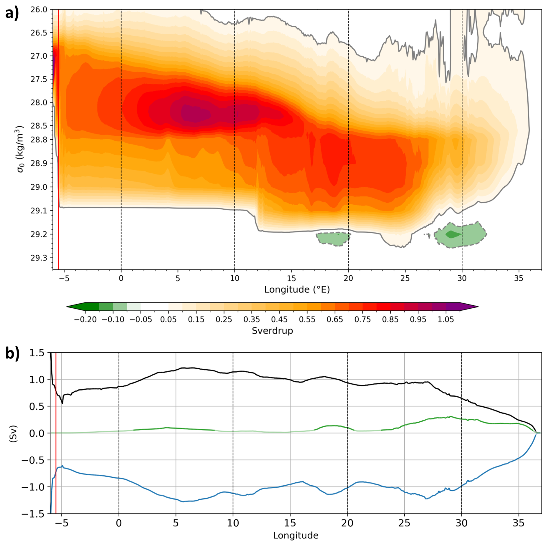
Figure 2 (a) Time-ensemble-averaged ZOC_σ as a function of longitude and potential density (σ₀). Density classes with transports smaller than 0.05 Sv are shown in white. The grey contour indicates −0.05 Sv (dotted line) and 0.05 Sv (solid line). (b) Mean transport of the surface (black), intermediate (blue), and bottom (green) zonal flows associated with the overturning cells, calculated from the differences ZOC${}_{\mathit{\sigma }}(max)-{\mathrm{ZOC}}_{\mathit{\sigma }}\left(\text{surface}\right)$, ZOC${}_{\mathit{\sigma }}(min)-{\mathrm{ZOC}}_{\mathit{\sigma }}(max)$, and ZOC${}_{\mathit{\sigma }}\left(\text{bottom}\right)-{\mathrm{ZOC}}_{\mathit{\sigma }}(min)$, respectively. Min and Max are calculated before the time-ensemble average, and so are not directly comparable with panel (a). Transparency indicates where time-mean zonal transports fall below 0.05 Sv. In both figures, the longitude of the Tarifa Narrows is shown as a red line.

3.1.2 Total variability (σ_T) of SSH

In both the observations and the simulations, the high-frequency (HF) total SSH variability reaches its maxima along the Algerian jet, and in the Levantine Sea (Fig. 1c, d). In these regions, the model slightly underestimates the observed HF total variability, as was reported by Beuvier et al. (2012) in a similar but non-ensemblist NEMO simulation; it is also possible in our case that the underestimation of local HF variability maxima is enhanced by the ensemble averaging process that smoothes out inter-member differences. Another discrepancy is found southeast of Crete, in the Ierapetra gyre, where the simulated HF variability is weaker than observed. On the opposite, HF variability maxima are simulated in coastal bands narrower than 100 km in the Gulf of Lions and of the Gulf of Gabès, which do not appear as clearly in the altimetric estimate whose effective resolution is likely too coarse. We will come back to the probable origin of these narrow bands in the following. Aside from these local differences, the model reproduces HF SSH variability reasonably well, with standard deviations of 3–4 cm matching observations.

The model correctly reproduces the low-frequency (LF) total SSH variability (Fig. 1e, f), capturing the main observed patterns and amplitudes. In particular, the North Ionian Gyre (NIG) stands out as one of the dominant modes of LF variability, both in the observations and the simulations. Observations reveal local LF variability maxima around the Cretan Sea, but their simulated counterparts appear too weak, suggesting a lack of energetic regional variability there. Conversely, the model overestimates the variability in the Balearic Sea (39.5° N; 2.5° E), as also reported by Waldman et al. (2018); Hamon et al. (2016) using earlier versions of the same model configuration. Based on these results, we excluded the Ierapetra, Pelops, and Balearic gyres from the subsequent analysis of vorticity in Sect. 4.2. These gyres either exhibit too small low-frequency variability in the observations, or significant discrepancies in their modeled representation–particularly in terms of amplitude and persistence. The five gyres retained for their subsequent analysis in terms of forced and intrinsic LF fluctuations are those that are correctly located and exhibit a substantial variability in both the simulated and observed datasets.

3.2 Zonal Overturning Streamfunction (ZOC) in density coordinates

ZOC represents the zonal transport cumulated from the densest waters up to a lighter density class. Its maximum along the density axis indicates at each longitude the intensity of the clockwise upper overturning cell, and its minimum at depth the intensity of the counterclockwise lower cell (where and when it exists). Depending on longitude, these two cells are associated with two or three opposite flows stacked vertically:

1. Surface eastward flow: its transport is given by the difference between the maximum of ZOC_σ and its value at the lightest density level (surface).

2. Intermediate westward flow: its transport is given by the difference between the ZOC_σ minimum in dense classes and its aforementioned maximum.

3. Bottom eastward flow: where it exists, its transport is given by ZOC_σ in the densest class (zero by construction) and the ZOC_σ minimum.

3.2.1 Time averaged ZOC_σ and zonal transports

Figure 2a shows the time-ensemble-mean zonal overturning circulation in density space in the basin. ZOC_σ reaches its maximum around 28.4 kg m⁻³ near 6° E and around 28.9 kg m⁻³ around 19° E. This limit marks the center of the clockwise upper overturning cell, and the lower boundary of its upper limb (surface eastward flow). Atlantic Waters (AW) crossing the Strait of Gibraltar are carried eastwards within this branch, get progressively denser during their journey as evaporation salinizes and cools them. In the eastern basin, most of the surface waters have become dense enough to sink and flow back underneath towards the Strait of Gibraltar, within the lower limb of this upper cell (intermediate westward flow). Part of these westward-flowing waters get lighter and are upwelled back into the upper limb in the western basin, but most of them cross the Straits and overflow into the Atlantic Ocean.

The simulated transports at Gibraltar are evaluated at the longitude of the Tarifa narrow (5.5° W), as done by Soto-Navarro et al. (2015). The time-ensemble-mean eastward transport of Atlantic waters is 0.79 Sv, close to the 0.85 ± 0.05 Sv estimate deduced by combining current meter observations and basin-scale mass balance (Gonzalez et al., 2025). The time-ensemble-mean deeper westward transport of Mediterranean waters is 0.74 Sv at the same longitude. This is also close to observed reconstructions, with an estimated outflow of 0.81 ± 0.05 Sv from INGRES measurements (Sammartino et al., 2015).

The time-ensemble-mean of the surface eastward transport (Fig. 2b) increases from about 0.74 Sv at Tarifa Narrows (5.5° W) to 1.2 Sv near 6° E (Gulf of Lions and Algerian basin), mostly due to the aforementioned upwelling of denser waters in the western basin (Waldman et al., 2018). This transport smoothly decreases between 6 and 15° E and remains close to 1 Sv up to 27° E; it decreases to zero in the easternmost part of the basin as this 1 Sv of AW sinks, ultimately feeding the westward-flowing intermediate layer. This latter transport shows overall consistent zonal variations with the surface eastward transport, the bottom transport being largely second-order west of 25° E.

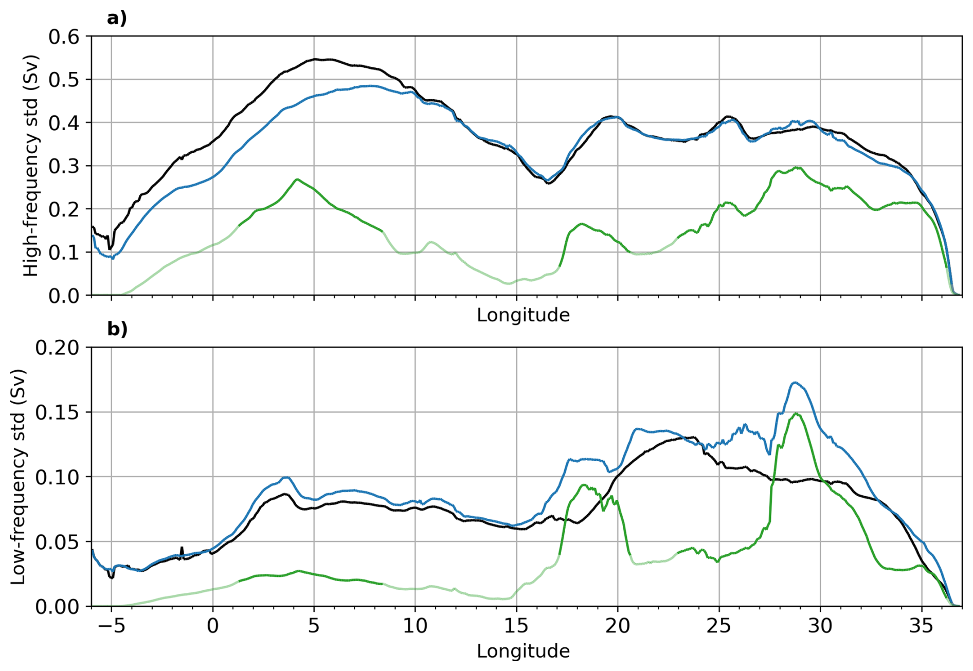
Figure 3 Standard deviation of the total variability of surface (black), intermediate (blue), and bottom (green) zonal transports at high-frequency (a) and low-frequency (b). Transparency indicates where time-mean zonal transports fall below 0.05 Sv.

The time-ensemble-mean ZOC_σ upper cell structure and amplitude are qualitatively – if not quantitatively – consistent with those described by Sayol et al. (2023) based on a $\mathrm{1}/\mathrm{12}$° reanalysis. Their Fig. 3c shows a similar basin-wide upper cell in density coordinates, with a similar zonal profile of the surface eastward transport. Our ensemble captures the longitudinal alternation of small transport maxima (associated with secondary overturning cells), with peaks located around 5 and 11° E in the western basin, and 17, 18.5, and 24° E in the eastern Mediterranean – slightly shifted eastward relative to the reanalysis. Another difference is found in the maximum density of the surface eastward flow in the western basin, which is about 0.3–0.4 kg m⁻³ smaller in our simulation than in the reanalysis, likely reflecting some differences in buoyancy forcing, convection patterns or water mass properties. Overall, the model shows good agreement with the representation of Atlantic inflow into the Mediterranean, the eastward transport of AW throughout its longitudinal range, and the rate and location of AW sinking throughout the basin.

Slightly negative ZOC_σ extrema are found at largest densities at certain deep locations east of 3° E; they correspond to the counterclockwise bottom overturning cell, which feeds the bottom eastward flow, and locally intensifies the westward intermediate flow. This lower cell, which is very likely influenced by dense water formation in the Gulf of Lions, Aegean Sea and Adriatic Sea, is weaker than the upper cell: its lower limb drives an eastward mean bottom transport of about 0.1 Sv around 4° E, 0.2 Sv at 19° E and 0.34 Sv at 29° E. Its upper limb slightly intensifies the intermediate westward transport with the same time-mean amplitude, thus explaining the slight asymmetry between the black and blue lines in Fig. 2b.

3.2.2 Total variability (σ_T) of zonal transports

The high-frequency standard deviation of the surface eastward and intermediate westward transports (Fig. 3a, blue and black lines) is of the same order of magnitude as their time-mean values (standard deviation of about 0.4 Sv and a mean value of about 1 Sv), indicating substantial HF fluctuations in the upper ZOC_σ cell. In the surface eastward branch, the HF standard deviation reaches its maximum (0.55 Sv) at 5° E, i.e. near the Gulf of Lions deep convection site, and remains close to 0.4 Sv from 19 to 31° E. Its low-frequency counterpart (Fig. 3b, black) is 3–5 times smaller, and exhibits an opposite zonal asymmetry with larger values in the eastern basin (up to 0.14 Sv at 23° E). This suggests that the atmospheric forcing and/or intrinsic ocean dynamics drive ZOC fluctuations with different time scales in both halves of the basin. This hypothesis is addressed in the next section, where total variability is split into forced and intrinsic components.

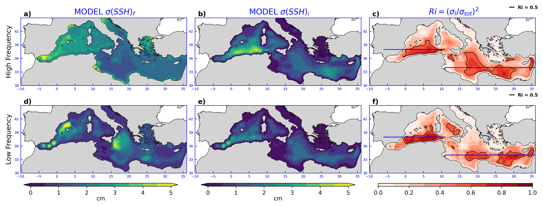
Figure 4 Forced and intrinsic standard deviations of the HF SSH variability (a, b) and of the LF SSH variability (d, e). The right column shows corresponding mean intrinsic variance ratios R_i defined in Sect. 2.3.4, at HF and LF (c, f); the black contour corresponds to R_i=0.5. Horizontal lines in panels (c) and (f) indicate the latitudes where SSH spectra are shown in Fig. 5 (see Sect. 4.1.3).

The total HF variability of the intermediate westward transport is about 20 % weaker than that of the eastward surface transport west of 10° E. This difference may be associated with the local maximum of HF variability of bottom eastward transport at 4° E. There, the instantaneous bottom transport can reach nearly three times its mean value, likely due to short and intense deep‐water formation events in the Gulf of Lions.

West of 10° E, the total HF variability of intermediate westward transports is smaller than that of surface eastward transport, suggesting that short-term anomalies of the upper and lower ZOC cells have the same sign (both clockwise or both counterclockwise). In the eastern basin, LF variability shows the opposite behaviour: intermediate transport fluctuations dominate over those at the surface, especially between 17–21 and 27–30° E, close to the Adriatic and Aegean deep convection sites. This suggests that long-term anomalies in the upper and lower ZOC cells often tend to have opposite signs, i.e. one clockwise and the other counterclockwise. These two longitude ranges are also those where low-frequency zonal transport fluctuations are weaker at the surface than at the bottom: intermediate zonal transports are thus mostly modulated there by the lower ZOC cell at low-frequency.

Explaining the dynamical origin of the signals described in this section lies beyond the scope of this study; these results however suggest that deep convection impacts zonal transport anomalies in contrasting ways depending on density, time scale, and longitude.

4 Contributions of forced and intrinsic variability

We have described at this point the total variability of our variables of interest in the simulation in comparison with available observations. We now take advantage of ensemble statistics introduced in Sect. 2.3.4 to split the simulated variability at various time scales into its forced and intrinsic components, and to compare them.

4.1 Sea Surface Height

The left and middle panels in Fig. 4 show the decomposition of the SSH variability into its forced and intrinsic components, at HF (top) and at LF (bottom).

4.1.1 High-frequency SSH variability

The forced high-frequency SSH variability (Fig. 4a) is strongest along the coasts. It reaches local maxima in the northeastern Aegean sea, in the Gulfs of Lions, Gabès and Venice, potentially favored by the concave geometry and shallow depth of these regions. SSH variability maxima may be driven by HF fluctuations of dominant winds in the latter regions (e.g. Tramontane, Mistral, Meltemi, Bora), as well as in the Alboran Sea subjected to fluctuations of the Levante and Poniente winds.

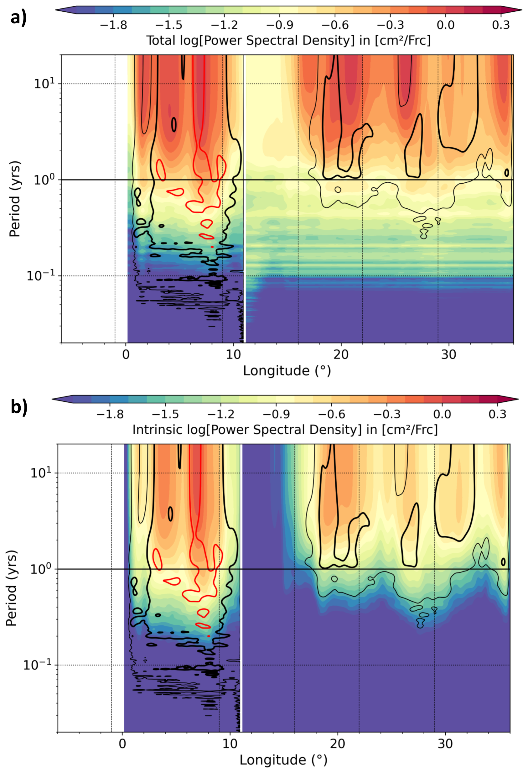
Figure 5 Colors show the logarithm of the Power Spectral Density (PSD) of total (a) and intrinsic (b) SSH variability as a function of longitude along the zonal lines shown in Fig. 4c, d. PSDs were computed within each member from 38-year deseasonalized and detrended daily SSH timeseries, without (a) and with (b) prior removal of their ensemble mean, and then ensemble averaged. PSDs are shown using a log10 scale (cm² day). The intrinsic-to-total PSD ratio is shown in both panels as 25 %, 50 %, and 75 % isolines (thin solid, thick black, and red contours, respectively). To improve readability, both PSDs were smoothed in the frequency domain using a 11-point Hanning window as done in Leroux et al. (2018).

Intrinsic HF variability exhibits a very different spatial distribution, likely associated with eddy-active regions along the Algerian coast, the Ionian Basin and in the Levantine Basin (Fig. 4b). The strong intrinsic HF signal along the Algerian coast likely reflects the combined effect of baroclinic instability and the interaction of currents with complex coastal topography (Puillat et al., 2002; Demirov and Pinardi, 2007). These processes can lead to the spontaneous generation of energetic mesoscale structures whose high-frequency random fluctuations are relatively independent of direct atmospheric fluctuations. A marked intrinsic signal is also found near 29° E–36° N, within the northern part of the Rhodes Gyre. Intrinsic HF variability remains negligible in shallow regions such as the Adriatic and Aegean Seas, the Gulf of Lions, and over the Tunisian shelf; the model resolution may not be fine enough there to resolve hydrodynamic instabilities because of small Rossby radii.

The HF intrinsic variance ratio is shown in Fig. 4c. A ratio of 1 indicates that variability is entirely intrinsic, and a value of 0 reflects purely forced variability. Intrinsic processes account for about 20 % of the HF SSH variance over the shallow coastal areas (Aegean Sea, Adriatic Sea, Tunisian shelf), and about 40 %–50 % in the central Mediterranean. The largest HF ratios are found along the Algerian coast (up to 60 %), in the Levantine Basin and in the South Ionian Sea.

4.1.2 Low-frequency SSH variability

Maxima in forced LF variability (up to 7 cm) are found in the Balearic, Alboran and Ionian Seas (Fig. 4d). In these regions, intrinsic LF variability is about 2–3 times smaller (2–3 cm, Fig. 4e), indicating that low-frequency SSH anomalies there are mostly driven by the atmosphere. This intrinsic LF component exhibits a more homogeneous distribution across the central and southern Mediterranean, with notable maxima east of the Alboran Sea and within the Algerian Basin, and remains small in most shallow regions as reported at HF.

However, the intrinsic component explains more than 50 % of the LF SSH variance in several regions, including the Algerian Basin, the Tyrrhenian Sea, the southern Ionian Sea, and the Levantine Basin. Altogether, these areas represent approximately 17 % of the total basin area both at HF and LF, and are located in the same regions at both time scales with two exceptions: R_i exceeds 50 % at LF and not at HF in the Tyrrhenian Sea, and the opposite is found in the central Ionian Sea. Considerable LF intrinsic variance ratios are found along the Algerian coast, where up to 75 % of the LF SSH variance is of intrinsic origin. Small intrinsic variance ratios characterize shallow regions, where the LF variability is thus mostly paced by the atmospheric forcing.

4.1.3 Spectral analysis of SSH variability

The variance maps presented above provide a spatial view of SSH variability in two wide classes of time scales. We now extend our analysis to the entire frequency spectrum by computing the power spectral density (PSD) of SSH variability components between 2 d and 18 years, focusing on two latitudes where R_i is largest: 38° N in the western basin and 34° N in the eastern basin (Fig. 4c, f). Colors in Fig. 5a and b show along this line the longitude-dependent PSDs of the total and intrinsic variability, respectively.

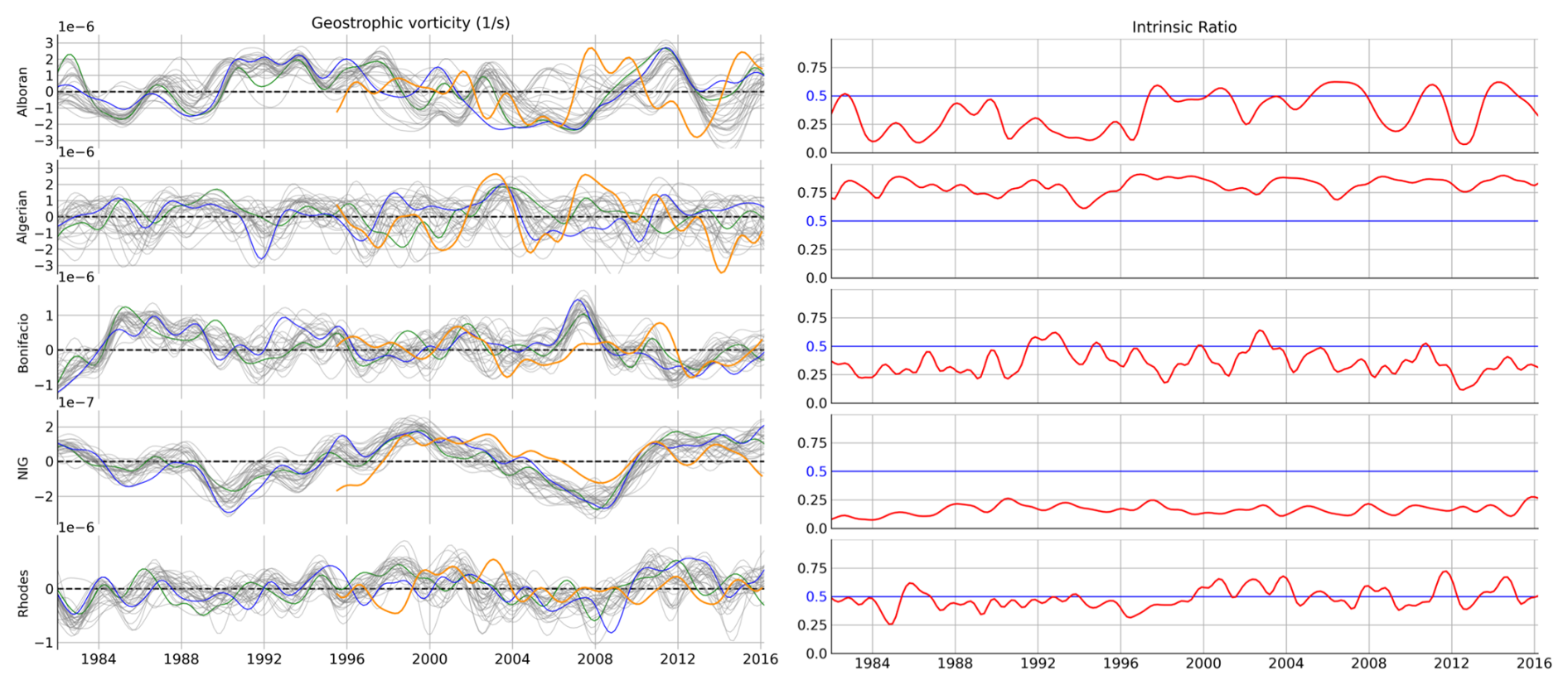
Figure 6 Left: low-frequency evolution of geostrophic vorticity anomalies within the boxes shown in Fig. 1, computed as explained in Sect. 4.2. Two randomly selected members are shown in blue and green, the remaining 28 ensemble members are shown in grey, and the vorticity derived from AVISO is shown in orange. Right: temporal evolution of the intrinsic variance ratio R_i(t) for each gyre. The blue line indicates the 0.5 threshold, above which intrinsic variability dominates.

The total and intrinsic SSH variability spectra are red throughout the basin. Consistently with Fig. 1d and f, the total spectrum shows moderate longitudinal contrasts at subannual periods at both latitudes, and localized peaks at periods longer than 1–2 years. The second spectrum reveals that high-frequency intrinsic variability (0.2–0.5 year periods) is much larger in the western basin where the 38° N line intersects the eddy-active Algerian current. More generally, the SSH intrinsic variability is strongest at periods longer than 1 year along both latitudes, except between 11 and 15° E above shallow topography south of Sicily.

The isolines in Fig. 5 represent the intrinsic-to-total PSD ratio. As for R_i, a ratio equal to 1 indicates that the variability at a given frequency and longitude is totally intrinsic, while a value of 0 corresponds to purely forced variability. More than 75 % of the SSH variability is paced by the atmosphere outside the thin black line (R_i<25 %), i.e. at subannual periods throughout the eastern basin and at all frequencies south of Sicily.

Thick black contours surround the frequency–longitude domains where intrinsic variability dominates, i.e. where SSH variability is mostly random. The clear dominance of intrinsic processes is striking in the western basin, particularly between 2 and 10° E at all periods longer than two months. The highest ratios are concentrated near 7° E, where more than 75 % of the SSH variance is random (red shading), at all periods ranging from 3–4 months to 2 decades. In the eastern basin, intrinsic variability plays a less dominant role overall but still accounts for a substantial fraction of the SSH variance; it explains at least 25 % of the SSH variability at periods longer than 5–12 months east of 18° E, and more than half of its interannual variance around 18–22 and 30–32° E.

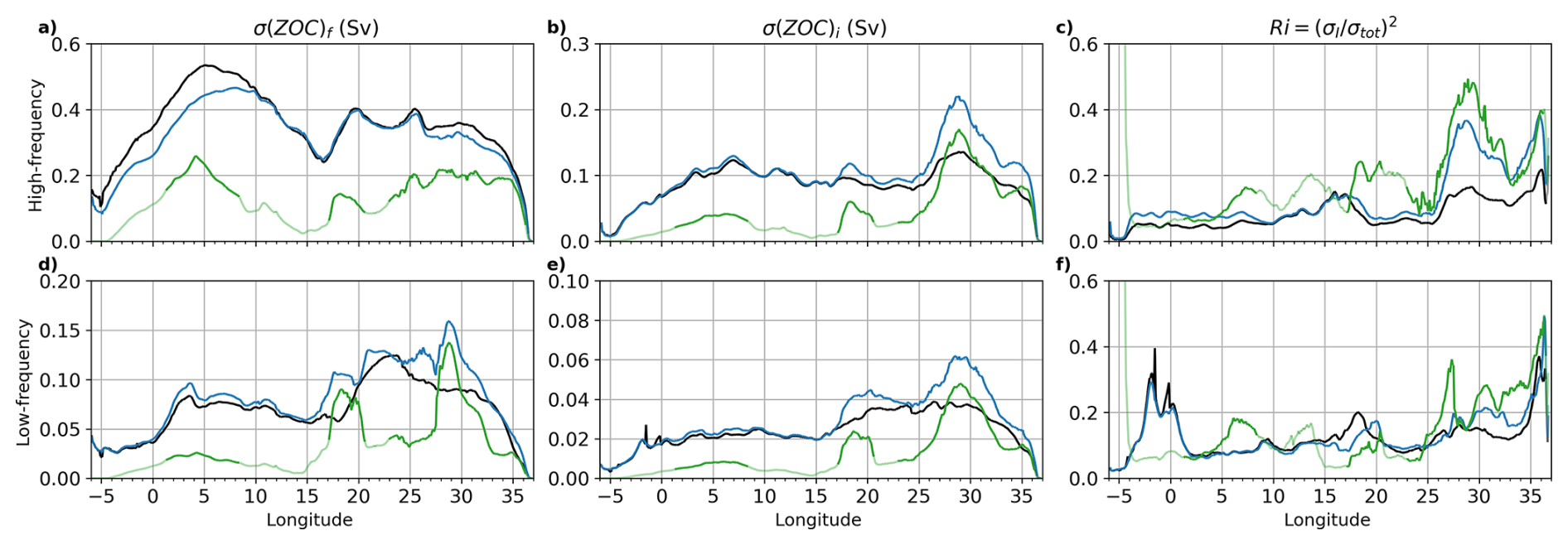
Figure 7 Forced (left) and intrinsic (middle) variabilities in Sv of the surface (black), intermediate (blue), and bottom (green) zonal transports at high (first line) and low (second line) frequency. Corresponding mean intrinsic variance ratios (R_i) are shown in the right panels. Color transparency indicates where time-mean zonal transports fall below 0.05 Sv.

4.2 Low-frequency modulation of regional gyres

We now turn our attention to the debated contributions of forced and intrinsic low-frequency variability on the NIG; these latter two contributions are examined within four other regional gyres as well, to assess the potential diversity of gyre dynamics across the basin (Fig. 1). The LF time series of their geostrophic vorticity relative to their temporal mean is shown for each member (left panels in Fig. 6), and reveals contrasting amplitudes and imprints of intrinsic variability within different gyres. A first indication of the model skill is given by the fact that the observed vorticity, shown in orange in the left panels, remains generally within the ensemble range (despite temporary exceptions, e.g. in 2007–2008 and 2012–2013 in the Alboran gyre). The right panels in this figure quantify the time-varying random character of these gyres' fluctuations. In particular, large R_i events indicate substantial phase differences between members, such as in the Algerian gyre around 1998 where the members shown in blue and green in the left panel generate opposite vorticity anomalies. The different phases of these gyres in various members clearly illustrate the advantage of ensemble over single simulations for attributing specific events to external drivers (also see Narinc et al., 2024).

• Eastern Alboran Gyre. the upper panels of Fig. 6 confirm the substantial imprint of intrinsic variability in this region, as already reported by Peliz et al. (2013). The intrinsic variance ratio R_i(t) exhibits strong temporal changes in this gyre: its LF variability is mostly forced over certain periods (e.g., 1990–1997) and intrinsic at other times (e.g., 1997–2008, 2011 and 2014). Hints of bimodal intrinsic behaviours also seem to appear in 2005–2008, when 5 members simulate positive vorticity anomalies, most others simulate the opposite, and a few switched modes.

• Algerian Gyre. In agreement with SSH diagnostics, the Algerian gyre LF vorticity fluctuations match AVISO in terms of amplitude, and remain strongly random during these 35 years (65 % $<R_{\mathrm{i}}\left(t\right)<\mathrm{90}$ %) despite the common external forcing and the tiny initial perturbations of our integration strategy.

• Bonifacio Gyre. The low-frequency fluctuations of this gyre are weaker and in relatively good agreement with AVISO in terms of amplitude, but not in terms of phase in 2007 and 2001. Its intrinsic variance ratio lies around 40 % (25 % to 55 %) suggesting oscillating contributions from external forcing and internal dynamics.

• North Ionian Gyre (NIG). As mentioned in the introduction, low-frequency modulations of the NIG vorticity are attributed to intrinsic variability by certain authors and to the atmospheric variability by others. The phase of the NIG vorticity anomalies is relatively well reproduced in our simulation, despite a small lack of amplitude (Fig. 6). Our model results suggest that this variability is weakly sensitive to CIV, as R_i(t) remains between 10 % and 25 % throughout the period. In other words, simulated NIG fluctuations are mostly paced by the atmospheric variability, as also suggested by Liu et al. (2022) with a different modeling approach. This result, however, does not explain the precise dynamics of this atmospheric influence, which is left for future studies. This result, however, does not explain the precise dynamics of this atmospheric influence, which is left for future studies.

• Rhodes Gyre. This easternmost gyre exhibits the smallest variability amplitude, roughly matching AVISO estimates. R_i(t) in this gyre remains close to 50 % throughout the period, suggesting a balanced contribution of forced and intrinsic processes in driving its inter-annual deviations.

These diagnostics thus reveal a wide range of gyre behaviours, from strongly forced (NIG) to largely intrinsic (Algerian gyre), and mixed regimes (Alboran, Bonifacio and Rhodes gyres), and highlight the need for dedicated sub-basin analyses.

4.3 Zonal transports

After presenting the imprints of forced and intrinsic variabilities on horizontal circulation patterns, we now assess their imprints on the three ZOC-derived meridionally-integrated zonal transports across the basin within various density ranges.

4.3.1 High-frequency variability of zonal transports

The forced and total HF variability of the surface eastward transport closely match each other (black lines in Figs. 3a and 7a), indicating the atmospheric pacing of most of its variance. Intrinsic variability remains modest (∼ 0.1 Sv, Fig. 7b), keeping R_i around 10 % throughout most of the basin. Similar values of R_i are found in the intermediate westward transport, except near 29° E where HF intrinsic fluctuations peak and raise R_i up to 37 % (blue lines in Fig. 7b–c).

In the western basin, forced HF fluctuations are slightly stronger at the surface than at the intermediate level (by about 0.05 Sv, Fig. 7a), suggesting positively-correlated, atmospherically-paced variations of the upper and lower ZOC cells. Intrinsic HF fluctuations exhibit the opposite pattern in the eastern basin, being larger at the intermediate level (Fig. 7b), which suggests anti-correlated random variations of the two cells (see Sect. 3.2.2).

The strongest HF intrinsic variance ratio is found in the bottom eastward transport (green line in Fig. 7c): R_i at 6 and 19° E is 2–3 times larger than in the upper branches, and reaches 50 % at 29° E. These localized maxima incidentally coincide with deep convection sites (Gulf of Lions, Adriatic and eastern Levantine basins), raising the hypothesis that the ensemble spread associated with short-term convection events (see Waldman et al., 2017) propagates downward and induce random HF transport fluctuations. Testing this hypothesis is left for future studies.

4.3.2 Low-frequency variability of zonal transports

Figure 7d–e shows that the forced and intrinsic LF variabilities of surface and intermediate transports are largest between 20 and 32° E, with more uniform and smaller amplitudes in the western basin. Forced fluctuations of both transports are smallest west of 1–2° W, probably since no LF variability is forced into the basin through the western buffer zone; this probably explains why intrinsic variance ratios R_i in the uppermost 2 layers reach a local maximum (about 30 %, black and blue lines in Fig. 7f) in the Alboran basin. Values of R_i decrease further east and get down to 10 % near 3° E, progressively increase again toward the east and reach another peak near 35° E.

The forced LF variability of bottom transports (green line in Fig. 7d) is maximum in the central and eastern basins, unlike its HF counterpart. In contrast, the LF intrinsic variability of bottom transports has the same zonal distribution as its HF counterpart with a 3–4 time smaller standard deviation. As at HF, the R_i of bottom transports at LF exceeds that of the other two layers east of 25° E, where 15 % to 50 % of the bottom transport variance has a random phase.

To summarize, the contribution of intrinsic processes on the HF and LF variance of zonal transports is globally largest in the eastern basin and in dense layers, with an additional maximum west of 3° E in the lightest two layers. More than 30 %–40 % of the variance of such transports can be random in phase locally, advocating for a more thorough analysis of their underlying dynamics, and for the need to keep in mind the importance of this intrinsic driver of random ZOC variability that competes with the atmospheric one.

4.3.3 Spectral analysis of intermediate transport variability

Figure 8a shows over the whole longitudinal and frequency domains the total variability of the intermediate westward transport. In accordance with Fig. 3a, the total variability PSD exhibits localized minima at the eastern end of the domain, around 26° E where topography is shallow, and at its western boundary where the lateral forcing is purely seasonal and intrinsic variability is damped. The intrinsic variability of this intermediate transport (Fig. 8b) reaches two maxima at LF in the eastern basin, in particular in the eastern Levantine basin, close to the Aegean convective site (26–29° E). In this longitude range, the intrinsic-to-total PSD ratio decreases with increasing time scales: above 50 % in the submonthly range, 30 %–50 % between 2 months and 2 years, and above 20 % up to 5 years.

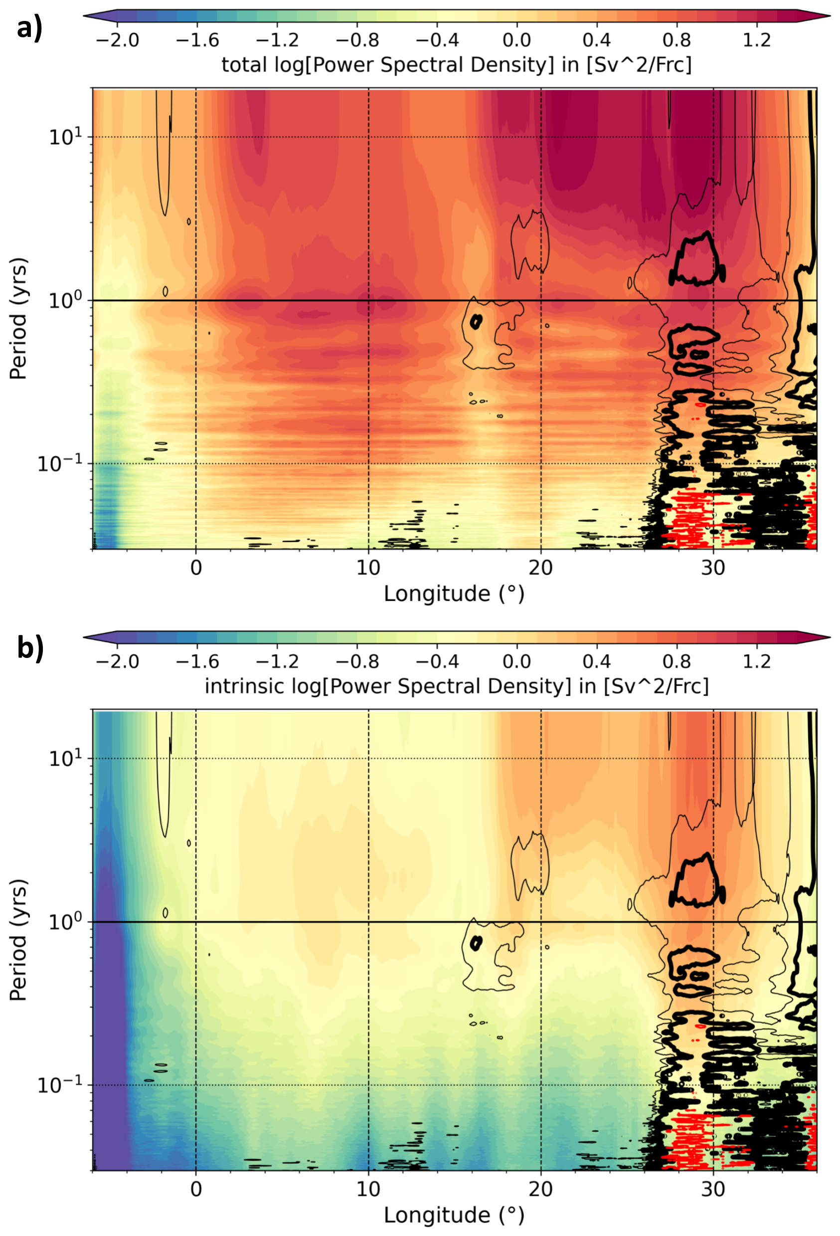
Figure 8 As Fig. 5 but for the intermediate transport variability (PSDs in color; units Sv² day). The intrinsic-to-total PSD ratio is shown as 20 %, 30 %, and 50 % isolines (thin solid, thick black, and red contours, respectively).

In the Ionian Sea (15–20° E) the intrinsic-to-total PSD ratio exceeds 20 % within the 5 months-3 year range. At 2° W in the Alboran Sea, this ratio exceeds 20 % at timescales longer than 4 years. We recall that all the results presented in this study only concern the intrinsic and forced components of the non-seasonal variability that is generated within the Mediterranean Sea: besides the climatological boundary forcing in the Gulf of Cadiz, no other potential influence of the Atlantic is injected into our domain.

5 Conclusions

This study explores from a 30-member ensemble $\mathrm{1}/\mathrm{12}$° simulation the respective imprints of the forced variability and of the chaotic intrinsic variability (CIV) in the Mediterranean Sea over the period 1979–2017. The forced variability is paced by the fluctuations of the external (atmospheric, river and lateral) forcing, while CIV spontaneously emerges from nonlinearities within the basin and has a random phase. We mainly focus on the surface circulation through SSH, and on the zonal transports within three layers associated with the density-coordinate overturning.

We evaluate the relative contribution of CIV on the variability of these fields at high and low frequencies (periods shorter and longer than about 2 years, respectively) using the metric R_i, the ratio between intrinsic and total variances, which varies between 0 (variability is fully forced) and 1 (variability is fully intrinsic).

Our analysis reveals that both high and low-frequency SSH fluctuations are mostly random (R_i>0.5) over 17 % of the Mediterranean Sea, in particular in the Algerian Basin, the southern Ionian Sea, and the Levantine Basin. The Algerian Basin is the main hot spot of Mediterranean intrinsic variability, where up to 80 % of the SSH variance is random at all periods between 4 months and 2 decades at least. Forced and intrinsic low-frequency variabilities have comparable amplitudes in the Rhodes, Bonifacio, and Alboran gyres; the relative contributions of both variability components substantially evolves in time in the latter gyre. In contrast, the simulated decadal fluctuations of the North Ionian Gyre are mostly paced by the atmosphere: less than 25 % of its low-frequency variance is intrinsic and random. This implies that, in this realistic simulation with fully varying air-sea fluxes, the timing of the observed reversals of the BiOS is mostly imposed by the atmosphere. This result contrasts with some previous studies based on observational data, idealized simulations, and laboratory experiments, which highlighted the potentially dominant role of CIV in NIG fluctuations (see introduction). Our simulation confirms that CIV has an impact on the NIG behavior, but suggests, as do other realistic ocean modeling studies, that taking into account complex stratification, basin geometry, and fully variable atmospheric variability gives more weight to external factors than to intrinsic processes in the timing of these fluctuations. Future studies will help further assess the robustness of these conclusions.

Between Gibraltar and about 25° E, the variability of the upper overturning cell, which is fed by the transport of Atlantic Waters (AW) to the east and of underlying intermediate waters to the west, is mostly paced by the atmosphere (and by the western boundary forcing at annual scale). However, an interannual-to-decadal intrinsic variability peak is found in the Alboran Sea within this upper cell, where R_i reaches 30 % for zonal transports in the surface and intermediate layers. East of 25° E, R_i increases only slightly in the surface transport, but reaches 35 %–40 % for intermediate layer transports in the Levantine basin (26–30° E) at timescales shorter than 3 years. This peak is due to a large maximum of intrinsic variability in the lower overturning cell, which strongly randomizes bottom and intermediate zonal transports.

Forced and intrinsic fluctuations of bottom transports, and of intermediate transports to a lesser extent, also happen to peak at all time scales near convection sites, i.e. near 29° E (eastern Levantine Basin), 18° E (western Ionian Basin) and 6° E (Gulf of Lions). These longitudinal correspondences raise the hypothesis that forced wintertime convection and associated intrinsic variability may have a specific impact on the lower overturning cell in these sites, in particular at 29° E where forced and intrinsic high-frequency variabilities have comparable influences (R_i∼30 %–50 %) on intermediate and bottom transports.

Our results extend over subannual and interannual time scales a previous basin-wide study of forced and intrinsic variability impacts at seasonal time scales (Benincasa et al., 2024). They also extend over the whole basin and over different variables a previous multi-scale analysis of forced and intrinsic variability impacts on deep convection in the Gulf of Lions (Waldman et al., 2018). This latter study highlighted the substantial imprint of multi-scale CIV on the volume of deep water formation, which might be related to the marked imprint of CIV on deep and intermediate advection via ZOC_σ-related flows in convection sites (see our Fig. 7b, c, e, f). A preliminary search of potential covariances between deep convection and zonal transports, and between horizontal and overturning circulations, did not reveal any simple and clear connections, though. A more thorough investigation of such hypothetical links should focus on forced and intrinsic variability mechanisms separately, which is left for future studies.

With a slightly different choice of filtering time scale, Carret et al. (2021) showed from the $\mathrm{1}/\mathrm{4}$° OCCIPUT ensemble simulation that interannual CIV has a very strong imprint on SSH in several regions of the global ocean (σ_i reaches 30 cm locally), but not in the Mediterranean Sea where σ_i reached modest maxima (about 1 cm) in the Alboran Sea and in the Algerian current. Maximum values of LF σ_i are found in the same area in our $\mathrm{1}/\mathrm{12}$° simulation, but they reach about 3 cm (Fig 4e). Such a 2 cm increase in LF σ_i was previously attributed to increased model resolution in the same region and across the basin (see the bottom panel of Fig. 10 in Sérazin et al., 2015), and presumably brings LF intrinsic variability to more realistic magnitudes at $\mathrm{1}/\mathrm{12}$°.

Whether intrinsic variability would further increase at even finer horizontal resolutions is very likely at mesoscale, but not certain in general: tripling the resolution of a global simulation did not significantly increase the Atlantic overturning interannual CIV (Grégorio et al., 2015). Assessing the robustness of the present results to model resolution and other parameters is left for future studies.

The spontaneous generation of multi-scale random fluctuations within the basin is a source of uncertainties that questions the attribution of regional fluctuations to sole atmospheric drivers, and that may hamper the predictability of its variability. Note that our experiment only gives access to the forced and intrinsic variabilities generated within the basin (as in most regional ensemble simulations, see e.g.  Lin et al., 2023; Jamet et al., 2020), and restricts the Atlantic influence to its mean seasonal cycle within the western buffer zone. It would be interesting in future experiments to inject through the western buffer zone the forced and intrinsic variabilities coming from the Atlantic (using e.g. the global OCCIPUT ensemble run outputs), and to assess within the Mediterranean basin the relative contributions of endogenous and exogenous variability sources.

The numerical model configuration used in this study however shows certain deficiencies in representing emblematic Mediterranean Sea features and events, such as the Eastern Mediterranean Transient, the Ierapetra anticyclonic gyre, or the North Balearic cyclonic circulation. This prevented us from drawing conclusions about the impact of intrinsic variability on these features, encouraging further studies with improved model configurations, ideally with ensemble integration strategies.

The imprint of multi-scale CIV in several parts of the Mediterranean Sea also has practical implications on modeling and observing the basin. Indeed, even a perfect model would most likely differ from observations in terms of phase in the presence of CIV.

On the one hand, this means that misrepresenting the phase of random events in an unassimilated single member simulation does not necessarily mean that the model is wrong. Ensemble simulations then provide modellers with an adequate means to explicitly represent and evaluate this stochasticity, and probabilistic assessment approaches that take all members into account may be used to robustly assess the skill of numerical models in the presence of this CIV-related uncertainty (see e.g. Narinc et al., 2024; Leroux et al., 2018) . On the other hand, observationalists could favor strategies that capture as completely as possible the statistics of key phenomena, that is to say with a long-term repetition of measurements at the same location. This argues to favor observations from anchored platforms such as buoys or moorings, whose time series are less challenging to interpret in the presence of CIV than those captured by moving platforms such as Argo floats or gliders.