Spatiotemporal scales of mode water transformation in the Sea of Oman

In the Sea of Oman, mode water forms at the surface and is trapped under a warm stratified layer in summer. This capped and well-mixed oxygenated layer decouples the oxygen minimum zone from ocean surface processes. It also provides a space for remineralisation, reducing oxygen demand in the oxygen minimum zone. Several physical processes, from isopycnal and diapycnal mixing to advection, transform mode water and change its properties. We perform a volume budget analysis to investigate the mechanisms driving mode water volume change in the Sea of Oman from monthly to 3 d temporal scales using monthly climatologies derived from profiling floats and high-resolution underwater glider observations. Isopycnal and diapycnal water-mass transformations are estimated in a density-spice framework. Our study shows that mode water predominantly transforms along isopycnals, yet strong but transient diapycnal transformation occurs at shorter timescales. Moreover, fluxes between the mode water layer and its surroundings are highly sensitive to the presence of mesoscale eddies. Across eddies, diapycnal and isopycnal transformations intensify by 61 % and 45 % respectively, compared to non-eddy conditions, indicating that eddies are drivers of both lateral and vertical water mass exchanges. This study provides a novel application of the water mass transformation framework to high-resolution underwater gliders, and shows that this methodology can be used at higher resolution than traditional climatological products or models. By comparing monthly climatological products to the high-resolution glider data, we suggest that the climatological estimates are outside of the high-resolution glider mean ± standard error 40 % of the time for diapycnal and 60 % of the time for isopycnal transformation. These results highlight the intense variability occurring at small scales and can serve to inform future estimates of water mass transformation uncertainty from coarser products.

1 Introduction

Mode waters are vertically homogeneous waters formed in the surface mixed layer and then subducted into the ocean interior (Hanawa and Talley, 2001). Surface water properties and tracers (e.g., heat, oxygen, organic matter) are trapped below the mixed layer during mode water formation. The seasonal variations of the mixed layer result in alternating mixing and stratification periods, trapping mode waters in the ocean subsurface, and favoring heat uptake, carbon sequestration, and oxygen ventilation (Lacour et al., 2023; Li et al., 2023; Portela et al., 2020a). Thus, mode water plays a crucial role as a pathway connecting the surface and subsurface ocean, influencing the distribution and transport of oxygen, heat, and remineralized organic matter.

In the Sea of Oman, mode water forms when springtime warming and weak turbulent fluxes stratify the surface layer and cap the deep surface mixed layer formed during the winter monsoon (Font et al., 2022, 2025; Senafi et al., 2019). The fate of mode water determines whether subducted surface properties are retained and transported into the ocean interior or mixed back into the surface mixed layer. This fate is governed by a variety of complex physical processes and instabilities that act at different spatial and temporal scales, resulting in diapycnal and isopycnal mixing and advection of mode water properties. Thus, these processes collectively regulate the transformation, ventilation, and residence time of mode water, thereby controlling its capacity to act as an oxygen reservoir (Kalvelage et al., 2015), or as a remineralization buffer layer (Weber and Bianchi, 2020).

In the Sea of Oman, mode water volume and residence time are among the largest within the Arabian Sea (thickness>50 m and residence time >4 months, Font et al., 2025), making it a key reservoir of oxygen. Mode water provides significant opportunities for the remineralization of labile sinking organic matter within this layer, reducing biological oxygen demand in the core of the oxygen minimum zone (Weber and Bianchi, 2020). Moreover, these are oxygen-rich waters, which can sustain the oxygen supplied to the upper oxygen minimum zone across the oxycline. It has been shown that, for instance, 50 % of the oxygen changes along mode water ventilation pathways are due to net community respiration within the water mass, the rest being due to mixing with surrounding oxygen-poorer waters (Jutras et al., 2025). Given their role in ocean heat uptake, biogeochemical cycling, and carbon sequestration, the life cycle of mode water and its changes have significant implications for both regional and global ocean-climate dynamics. Understanding the physical processes that mix and stratify mode water across scales, and how these processes interact with biogeochemical dynamics, is critical. While Font et al. (2025) provide valuable estimates of mode-water volume and residence time, the subseasonal and small-scale variability that governs changes in its properties remains poorly constrained, largely because observations at the necessary spatiotemporal resolution are still scarce.

Based on the method first introduced by Walin (1982) to compute water-mass transformation in thermohaline coordinates, we use a density-spice (σ-τ) framework (Portela et al., 2020b) to investigate volume changes at timescales, from daily to monthly, of mode water in the Sea of Oman leveraging high spatio-temporal resolution from underwater glider observations and Argo monthly climatologies. Potential density is used because it is materially conserved under adiabatic and isohaline motions and therefore provides a practical approximation to separate isopycnal and diapycnal fluxes, while spice is added as a second dimension in the volume budget to identify different water masses spreading along isopycnals (Jackett and McDougall, 1985; McDougall and Krzysik, 2015). Spice acts as a tracer of thermohaline changes along isopycnals, enabling the identification of water masses that are indistinguishable in density but differ in origin or transformation history. The water mass transformation framework has been widely employed to quantify how water masses change properties over seasonal to interannual timescales, often using Argo float data or numerical models (Badin et al., 2013; Evans et al., 2014; Nurser et al., 1999; Portela et al., 2020b). These studies reveal gradual seasonal transformation driven by surface fluxes and large-scale circulation. However, evidence highlights the significant contribution of mesoscale eddies and other transient processes to shorter-term variability and transformation events (e.g., Liu and Li, 2013; Shi et al., 2018; Trott et al., 2019; Thoppil, 2024; Xu et al., 2016). Our approach and a high-resolution dataset allow us to capture the episodic and localized transformations often missed by coarser-resolution climatologies and models, to resolve short-term drivers of isopycnal and diapycnal change.

Specifically, this study addresses the following key questions: (1) How does mode water change across different timescales, from days to seasons? (2) Which physical mechanisms predominantly drive mode water transformations in the Sea of Oman? By combining glider data with climatological products, we provide a quantitative assessment of water mass transformation dynamics of this layer with important biogeochemical regional implications.

Figure 1 Data distribution. (a) Sea of Oman colored by the number of Argo profiles per 0.25°×0.25° geographical grid. Land is shaded gray, the coastline is marked as a solid line, and the contours of the 100 m and 1000 m isobaths are dotted. The dashed orange line is the transect across the Sea of Oman where Argo profiles are projected to. The glider transect is marked with the black line, and its duration is colored in black in the time bar. (b) Yearly and (c) monthly distribution of the number of Argo profiles in the Sea of Oman. (d) Monthly climatological stratification (Brunt-Vaisala frequency squared, N²) profiles from Argo data. (e) Stratification time series of the upper 200 m from the glider data. The white solid line is the mixed layer depth, the upper and lower boundaries of the mode water layer (25 and 25.25 kg m⁻³ isopycnals, respectively) are marked with white dotted contours, and the yellow dashed line is the 60 µmol kg⁻¹ oxygen contour. Note that after May, no more oxygen data are available due to sensor failure.

2 Data and methods

2.1 Ocean glider observations and Argo climatology

We utilized four months of glider observations sampling across the continental shelf in the southern Sea of Oman. The Seaglider carried out repeated sampling along an 80 km transect between 23.65° N, 58.65° E and 24.25° N, 59° E in 2015 (Fig. 1a). Observations were projected onto a straight across-shelf transect (Fig. 1a, black line) and median-binned onto a 0.5 m (vertical) and 2 km (horizontal) grid. The origin of coordinates was taken at the 300 m isobath. Binned sections were interpolated vertically (1 m), then horizontally (4 km) to fill minor gaps, and smoothed horizontally with a 6 km running mean. The 6 km running mean is selected as a compromise between filtering out submesoscale variability (≲O(10 km)) and preserving mesoscale structures (≳O(20 km), comparable to the local Rossby radius). Mixed layer depth was defined using a potential density threshold of 0.125 kg m⁻³ relative to the surface (Font et al., 2022). Spice (τ; kg m⁻³) was computed from Conservative Temperature (Graham and McDougall, 2013; McDougall, 2003) and Absolute Salinity (McDougall et al., 2012) following the TEOS-10 routines (gsw_spiciness0, McDougall and Barker, 2011). Potential density and spice are referenced at 0 dbar. Eddy kinetic energy (EKE) was estimated from two independent sources: (1) the depth-averaged currents (DAC) derived from the glider flight model as $\text{EKE}=(\text{DAC}-\stackrel{\mathrm{‾}}{\text{DAC}}{)}^{\mathrm{2}}$, where $\stackrel{\mathrm{‾}}{\text{DAC}}$ is the mean DAC during the glider campaign (Frajka-Williams et al., 2011); and (2) from sea surface height-derived surface geostrophic velocities from satellite (CMEMS, 2025). EKE is defined as ${u^{\prime }}^{\mathrm{2}}+{v^{\prime }}^{\mathrm{2}}$; where $u^{\prime }=u-\stackrel{\mathrm{‾}}{u}$ and $v^{\prime }=v-\stackrel{\mathrm{‾}}{v}$ are respectively the zonal and meridional velocity time anomalies, where u and v are the surface geostrophic velocities at the glider transect location and $\stackrel{\mathrm{‾}}{u}$ and $\stackrel{\mathrm{‾}}{v}$ are the mean surface geostrophic velocities during the glider-sampling period. Mesoscale eddies in the region were identified using the ToEddies dataset, which applies an eddy detection algorithm to satellite-derived Absolute Dynamic Topography (ADT) fields (Laxenaire et al., 2024). The dataset provides daily information on eddy properties, including polarity, center location, and spatial extent (Laxenaire et al., 2024; Ioannou et al., 2024).

In addition, we used a total of 3565 Argo profiles of temperature, salinity, and pressure between 2000 and 2023 in the Sea of Oman (22.5–26° N, 56–61° E, Fig. 1a). Only profiles flagged as “good” by the CORIOLIS Data Centre were used (Gaillard et al., 2009). Argo float coverage spans the entire domain, with an average density of 28 profiles per 0.25°×0.25° grid cell (Fig. 1a) and a relatively uniform monthly distribution (Fig. 1c). Argo profiles within a 200 km distance from the across-Sea of Oman transect (Fig. 1a, orange dashed line) were selected. This strategy ensures sufficient monthly sampling coverage in this sparsely observed region to construct an across-gulf monthly climatology. Moreover, to avoid the influence of shallow profiles on the continental shelf, profiles shallower than 1000 m were excluded, so the transect remains representative of the environment where mode water forms and persists. Each profile was then orthogonally projected onto the nearest point along the transect (the orange dashed line in Fig. 1a), which provides its along-transect coordinate. Profiles were vertically interpolated onto a uniform 2 m pressure grid, and all projected profiles were median-binned into 3 km horizontal bins along the transect. Averaging was performed on pressure levels. Monthly climatologies were produced by taking the median across all profiles within each (depth, distance) bin for each month between 2000 and 2023. This gridded product is then used as input for the σ-τ water-mass transformation calculations.

We defined the mode water core as the layer bounded by the 25 and 25.25 kg m⁻³ isopycnals, which effectively capture the low-stratification and low-potential vorticity typical of mode water. This density-based definition closely aligns with a more traditional identification based on potential vorticity (Feucher et al., 2022; Herraiz-Borreguero and Rintoul, 2011; McCartney, 1982), as demonstrated by a strong correlation between potential vorticity and the potential density threshold method (see Fig. S1 in the Supplement, mode water thickness correlation between methods is r²=0.96). Using a fixed isopycnal threshold simplifies the interpretation of water mass transformation processes within the σ-τ framework (see Sect. 2.2), while remaining consistent with dynamically meaningful definitions of mode water.

2.2 Water mass transformation framework

The analyses are performed in σ-τ coordinates since: (1) potential density is the natural coordinate to study ocean dynamics and provides information about the diapycnal nature of the mechanisms driving the volume change; and (2) spice is interpreted as a measure of thermohaline variability along isopycnals, reflecting isopycnally-compensated temperature and salinity changes associated with the spreading of distinct water masses (Jackett and McDougall, 1985; McDougall and Krzysik, 2015).

Based on the constructed Argo monthly climatology and the ocean glider dataset, we performed a volume budget in σ-τ coordinates for the interior ocean (i.e., below the mixed layer). The water-mass volume change $\mathrm{d}V/\mathrm{d}t$ results from the sum of water-mass transformation, $\sum U(\mathit{\sigma },\mathit{\tau }$), and the exchange flux across the domain's geographical limits Ψ (Fig. 2a and Eq. (1), Evans et al., 2014; Portela et al., 2020b). U is the water-mass transformation due to isopycnal and diapycnal mixing fluxes, whereas its convergence or divergence is represented by the sum (∑) of the interior fluxes across the geographical limits of a given a σ-τ class (Donners et al., 2005; Walin, 1982). The isopycnal and diapycnal transformation rates represent the net mixing of water masses along and across density surfaces, respectively, resulting in an irreversible property change. Ψ represents the net exchange across the northern boundary of the domain, defined as the northernmost bin of the glider and climatology transect. Since the southern end is shelf-constrained, cross-section exchange there is assumed to be negligible. Note that an underestimation of the exchange flux Ψ could result in an apparent overestimation of the local transformation rate U. However, since both diapycnal and isopycnal transformations are estimated using the same underlying framework, there is no reason to expect a preferential bias toward either component. A diagram illustrating how changes in water characteristics are represented in σ-τ space is shown in Fig. 2a. The processes that modify the volume of a σ-τ class are depicted in geographical coordinates in Fig. 2b and c. The σ-τ class highlighted with a square in Fig. 2a is marked with dots in Fig. 2b and c. In summary, changes in volume within a given σ-τ class can be attributed to the convergence or divergence of interior fluxes across σ or τ boundaries, or via exchange fluxes across the domain boundaries within the same σ-τ class. Unlike interior mixing, exchange fluxes do not imply a transformation of water mass properties.

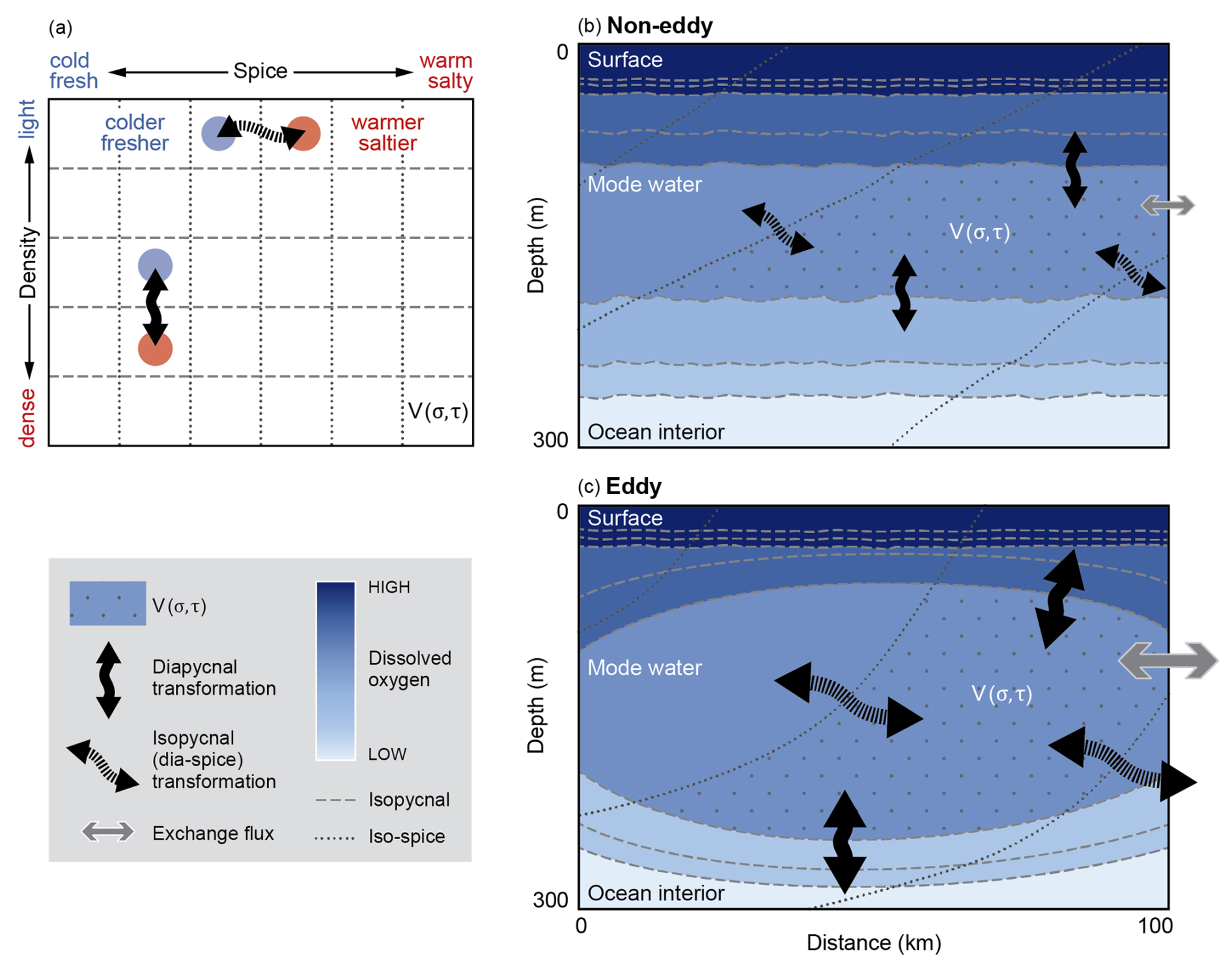
Figure 2 Water mass transformation framework for eddy and non-eddy sections. (a) Diagram showing the effect of the transformation of a given water class in σ-τ space (adapted from Fig. 1a from Portela et al., 2020b), and (b, c) processes involved in the volume change of a given σ-τ class in geographical coordinates for (b) a non-eddy and (c) an eddy section colored by dissolved oxygen concentration.

The method used here to compute water-mass transformation in the σ-τ coordinates is based on Portela et al. (2020b) and Evans et al. (2014). The volume change within a given σ-τ class can be expressed as:

$$\begin{array}{}\text{(1)}& {\displaystyle \frac{\mathrm{d}V}{\mathrm{d}t}}({\mathit{\sigma }}^{\prime },{\mathit{\tau }}^{\prime })=U_{\mathit{\sigma }}({\mathit{\sigma }}^{\prime },{\mathit{\tau }}^{\prime })+U_{\mathit{\tau }}({\mathit{\sigma }}^{\prime },{\mathit{\tau }}^{\prime })+\mathrm{\Psi }({\mathit{\sigma }}^{\prime },{\mathit{\tau }}^{\prime })\end{array}$$

where

$$\begin{array}{}\text{(2a)}& {\displaystyle }{U}_{\mathit{\sigma }}(\mathit{\sigma },\mathit{\tau })={\int }_{{\mathit{\sigma }}^{\prime }=\mathit{\sigma }}\mathrm{\Pi }(\mathit{\tau },{\mathit{\tau }}^{\prime })\cdot u_{\mathit{\sigma }}\cdot \mathrm{d}A\text{ and}\text{(2b)}& {\displaystyle }{U}_{\mathit{\tau }}(\mathit{\sigma },\mathit{\tau })={\int }_{{\mathit{\tau }}^{\prime }=\mathit{\tau }}\mathrm{\Pi }(\mathit{\sigma },{\mathit{\sigma }}^{\prime })\cdot u_{\mathit{\tau }}\cdot \mathrm{d}A;\end{array}$$

where u_σ and u_τ are the diapycnal and isopycnal (diaspice) velocity components, respectively, and dA is the cross-sectional area of the transect occupied by water within the specified σ-τ class. Π is defined as

$$\begin{array}{}\text{(3)}& \mathrm{\Pi }(\mathit{\sigma },{\mathit{\sigma }}^{\prime })=\mathrm{\Pi }(\mathit{\tau },{\mathit{\tau }}^{\prime })=\left\{\begin{array}{ll}\mathrm{1}& \text{if }\mathit{\sigma }\in {\mathit{\sigma }}^{\prime }\text{ and }\mathit{\tau }\in {\mathit{\tau }}^{\prime }\\ \mathrm{0}& \text{otherwise.}\end{array}\right.\end{array}$$

where ${\mathit{\sigma }}^{\prime }=(\mathit{\sigma }\pm \mathrm{\Delta }\mathit{\sigma }/\mathrm{2}$) and ${\mathit{\tau }}^{\prime }=(\mathit{\tau }\pm \mathrm{\Delta }\mathit{\tau }/\mathrm{2}$) and determines if a water parcel falls into a chosen σ-τ class. The volume integration was made in σ-τ classes with density intervals of 0.05 kg m⁻³ between 23–27.5 kg m⁻³ and spice intervals of 0.1 kg m⁻³ between 4–8.5 kg m⁻³. This choice reflects a trade-off between adequately representing each water mass class and ensuring that the mode water layer is well resolved.

Using Eq. (1), a set of linear equations can be generated to equate the volume trend and the interior water-mass transformation in σ-τ coordinates as $\mathrm{d}\mathbf{V}/\mathrm{d}t=\mathbf{A}\mathit{x}$, where $\mathrm{d}\mathbf{V}/\mathrm{d}t$ is the observed change in volume of each sigma-spice class, divided by the relevant time interval; A is the matrix of coefficients of the linear equations; and x is the vector of the resulting diasurface transformations and exchange flux. This system is solved by means of a least squares regression for the unknown transformation and exchange flow. The detailed methodology can be found in Sect. S1 in the Supplement. The solution x was then decomposed into the transformation across spice and density surfaces and the exchange flux across the geographical domain.

The volume of water bounded by a given tracer iso-surface (e.g., here σ or τ ) can change due to mixing across the tracer iso-surface or due to volume transport into or out of the domain. However, it can also change by air-sea buoyancy fluxes if the tracer surface outcrops at the ocean surface (Evans et al., 2014, 2023; Groeskamp et al., 2019). To assess the role of surface forcing, we applied the water mass transformation framework in temperature-salinity (T-S) space (Evans et al., 2014, 2023). Using glider and Argo T-S observations, together with ERA5 air-sea buoyancy fluxes (Hersbach et al., 2020), we diagnosed the surface transformation of distinct T-S classes, thereby identifying which classes are actively transformed by air-sea fluxes. These classes were mapped into σ-τ space and compared with the σ-τ domain of the mode water (Fig. S2), showing no overlap. The classes influenced by surface fluxes lie well above the density range of the mode water (Fig. S2), indicating that surface buoyancy forcing does not influence the observed mode water transformations. Moreover, we exclude a subduction term through the base of the deepest mixed layer (in contrast to Portela et al., 2020b). This is justified because we start the water-mass transformation analysis well after mode waters are capped and the σ-τ classes lie well below the surface mixed layer under strong stratification ($O\left({\mathrm{10}}^{-\mathrm{3}}\right){\mathrm{s}}^{-\mathrm{2}}$).

The water-mass transformation framework was applied to 20 repeated ocean glider sections, each 60 km long and extending from the surface to 500 m depth, at the location indicated in black in Fig. 1a. To minimize the influence of shelf processes on the transformation, sections begin 10 km from the 300 m isobath, where depths exceed 500 m. The temporal resolution is approximately 3 d between successive sections. The first transect included in the analysis starts on 25 March, roughly a week after restratification, to minimize the influence of potential subduction/exchange with the surface mixed layer. Moreover, the framework is also applied to the across-gulf monthly climatology to obtain a climatological average of water mass transformations in the region. As restratification of the surface mixed layer typically completes by mid-March (Font et al., 2022), we restrict the analysis of monthly transformations to the period from April onwards. The residual errors for both datasets, computed as ($|\mathrm{d}\mathbf{V}/\mathrm{d}t-\mathit{A}\mathit{x})|/|(\mathrm{d}\mathbf{V}/\mathrm{d}t)|$, were on average of order 10⁻⁵, which is on the higher end of values reported in previous studies (e.g., Portela et al., 2020b).

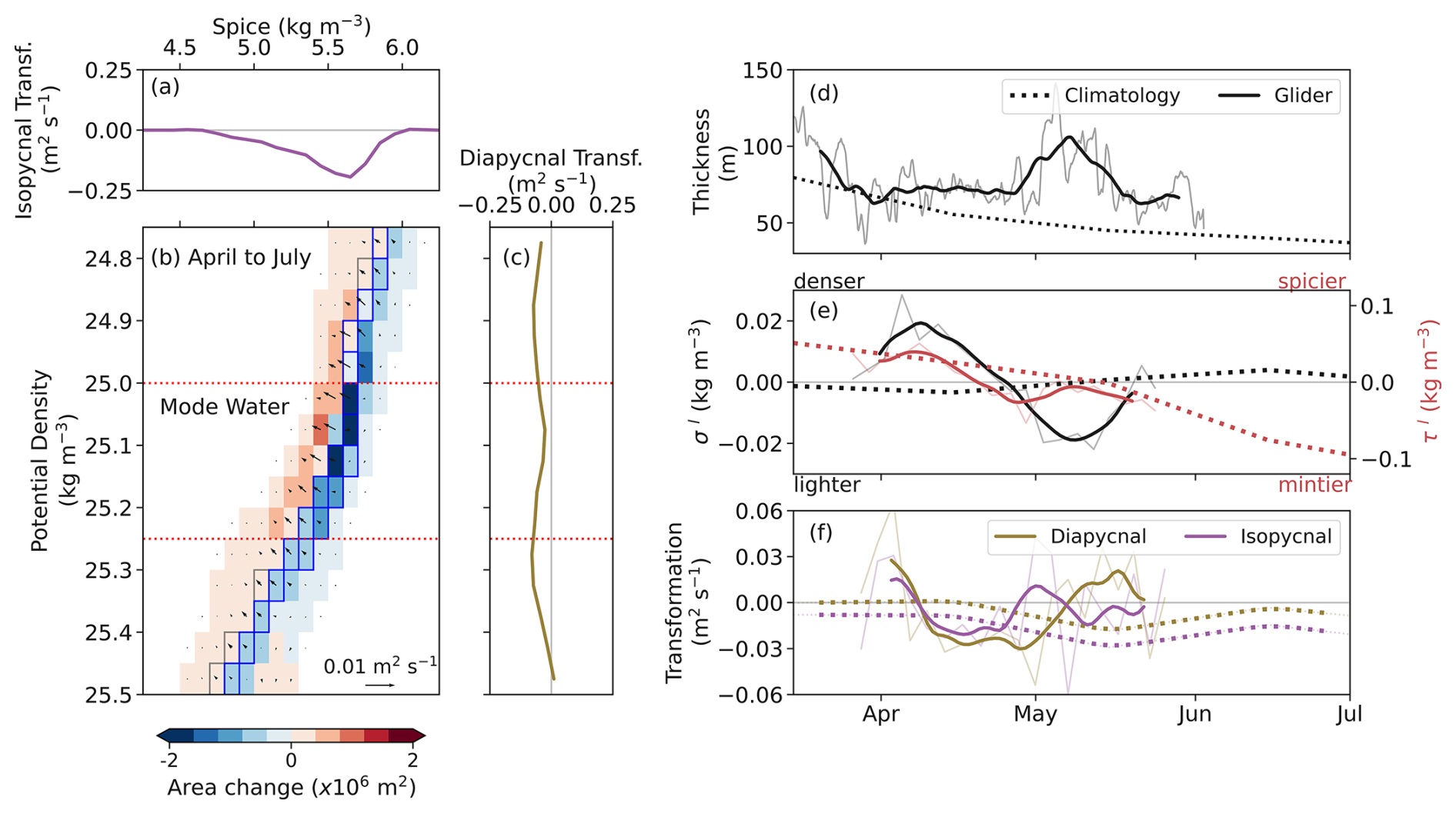
Figure 3 Timescales of mode water transformation. (a) Integrated isopycnal transformation per spice class from panel (b). (b) Climatological area changes between April and July. Arrows depict the transformation direction and magnitude per σ-τ water class. Mode water band (σ: 25–25.25 kg m⁻³) is delimited between the horizontal red dotted lines in panels (b) and (c). The σ-τ classes at the domain's boundary, thus, subjected to exchange flux, are marked with squares, colored blue when contributing more than 25 % of the area loss, and red when contributing more than 25 % of the area gain. (c) Integrated diapycnal transformation per potential density class from panel (b). (d) Mode Water thickness from glider data (solid gray), after applying a 24 h rolling mean (solid black), and the climatology (dotted). (e) Temporal anomalies of potential density (σ^′) and spice (τ^′) computed as deviations from their time-mean over the March–July period as ${\mathit{\sigma }}^{\prime }\left(t\right)=\mathit{\sigma }\left(t\right)-\stackrel{\mathrm{‾}}{\mathit{\sigma }}$ and ${\mathit{\tau }}^{\prime }\left(t\right)=\stackrel{\mathrm{‾}}{\mathit{\tau }}$ where $\stackrel{\mathrm{‾}}{\mathit{\sigma }}$ and $\stackrel{\mathrm{‾}}{\mathit{\tau }}$ are the time-means computed over the analysis period. Solid light lines show the 3 d glider anomalies; solid dark lines show the glider anomalies after applying a 10 d rolling mean; dotted lines show the monthly climatological anomalies. (f) Integrated diapycnal transformation (brown) and isopycnal transformation (purple) for mode water (σ: 25–25.25 kg m⁻³), from glider data (solid light), the glider after applying a 10 d rolling mean (solid), and the climatology (dotted).

3 Results

3.1 Timescales of transformation of mode water

We examine the seasonal-scale evolution of mode-water properties and transformations using the monthly Argo climatology (April–July). This climatological view captures the broad, low-frequency changes as the mode water evolves through late spring and early summer, but necessarily smooths over shorter-term variability. Mode water forms between February and March, and lingers as a homogeneous layer below the seasonal pycnocline (Fig. 1d and e), forming a boundary between the mixed layer above and the Arabian Sea oxygen minimum zone below ($<\mathrm{60}\mathrm{\mu }\mathrm{mol}{\mathrm{kg}}^{-\mathrm{1}}$) (Fig. 1e). Climatologically, the low stratification characteristic of mode water in the Sea of Oman is present until June (Fig. 1d), but it can persist longer inside eddies (Font et al., 2025; Liu and Li, 2013). Over seasonal timescales, the transformation framework reveals a net shift toward mintier (i.e., fresher and colder) and lighter waters, driven by negative isopycnal and diapycnal transformations (Fig. 3). Isopycnal transformation (Fig. 3a) indicates mixing into colder, fresher classes, while diapycnal transformation (Fig. 3c) reflects mixing into lighter classes. On average, the isopycnal transformation dominates ($-\mathrm{0.015}\pm \mathrm{0.009}{\mathrm{m}}^{\mathrm{2}}{\mathrm{s}}^{-\mathrm{1}}$), with a magnitude approximately three times larger than the diapycnal transformation ($-\mathrm{0.005}\pm \mathrm{0.008}{\mathrm{m}}^{\mathrm{2}}{\mathrm{s}}^{-\mathrm{1}}$) (Fig. 3a, c, and f). The signs of the transformation terms reflect the direction of the fluxes between density and spices classes, whereas the net Δσ and Δτ reflect the evolution of the volume-weighted mean properties. Thus, there is mode water volume formed due to transformation from lighter and mintier waters (red shading, Fig. 3b), but a large destruction predominantly in the lighter and spicier classes of mode water (blue shading, Fig. 3b). This fact, alongside a thinning of the mode water layer (ΔThickness=10 m per month, Fig. 3d), results in mean mintification and densification of mode water between March and June ($\mathrm{\Delta }\mathit{\tau }=-\mathrm{0.03}\mathrm{kg}{\mathrm{m}}^{-\mathrm{3}}$ per month, $\mathrm{\Delta }\mathit{\sigma }=\mathrm{0.0013}\mathrm{kg}{\mathrm{m}}^{-\mathrm{3}}$ per month, Fig. 3e).

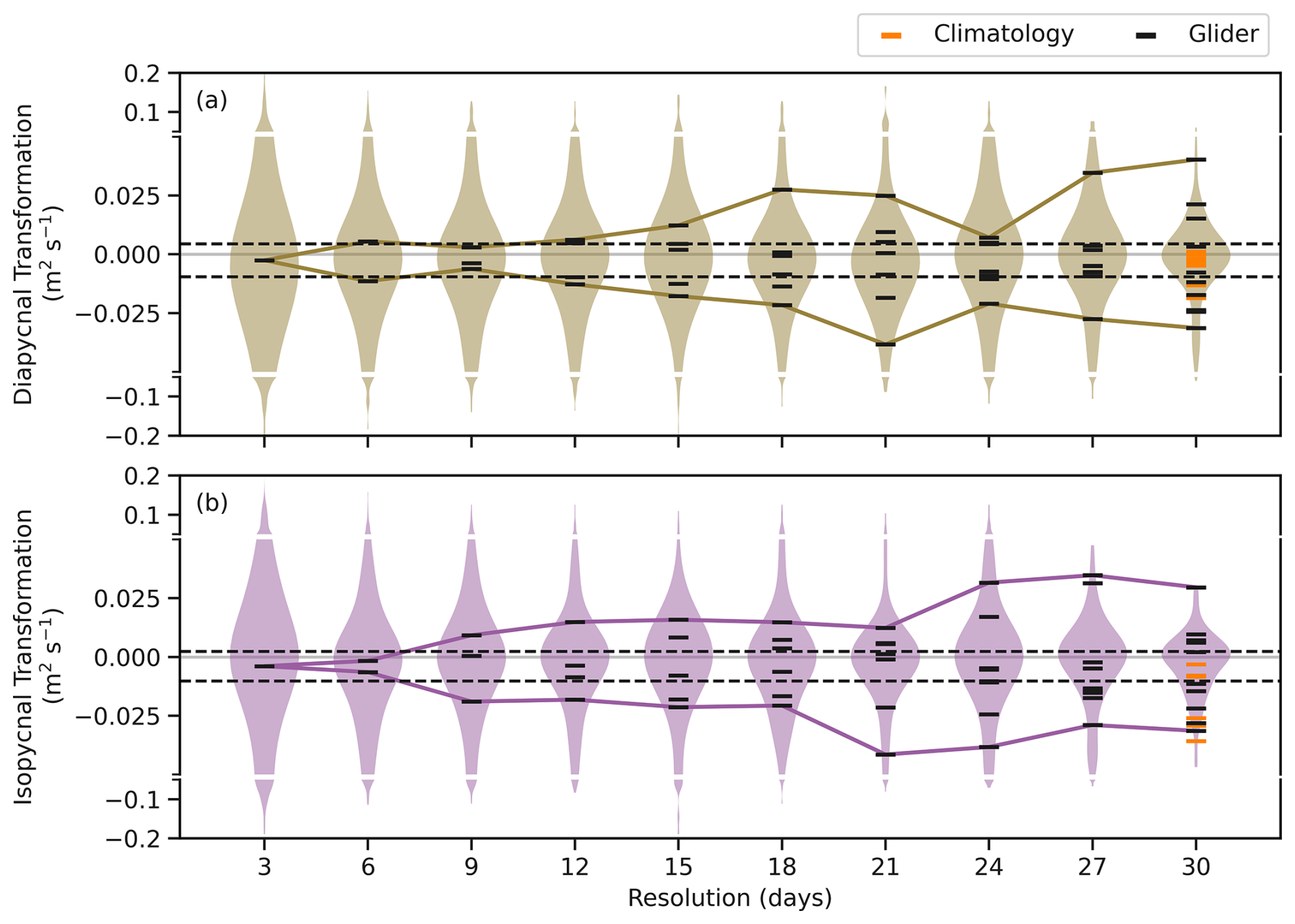
Figure 4 Sensitivity of mean transformation estimates to sampling resolution. (a) Diapycnal and (b) isopycnal transformations distribution after smoothing the transformation with a resolution-day rolling mean as violin plots. Lines (–) indicate mean transformations estimated from sub-sampling the 3 d time series at coarser intervals (resolutions): black for the glider dataset, and orange for the climatological dataset. The coloured line envelopes the minimum and maximum mean transformations from sub-sampling the time series, and the black dashed lines indicate the transformations within the mean ±1 standard error of the highest resolution (3 d).

The previous analysis was based on monthly climatologies and, therefore, mesoscale and smaller scale contributions to the transformation are largely averaged out. In contrast to the climatological perspective, the high-resolution glider time series resolves submonthly variability and therefore reveals the episodic, intraseasonal changes in mode water structure and transformations that are absent from the monthly climatology. This allows us to directly quantify short-lived events associated with transient processes, such as mesoscale eddies. Over shorter timescales, the high-resolution time series provided by the ocean gliders offers a unique view that highlights the large variability of mode water thickness and depth due to eddy presence and topographical interactions with the shelf break (Figs. 1e and 3d). We observe a transition toward mintier waters throughout the study period ($\mathrm{\Delta }\mathit{\tau }=-\mathrm{0.04}\mathrm{kg}{\mathrm{m}}^{-\mathrm{3}}$ per month), albeit with notable temporal variability as indicated by the sign changes in the isopycnal transformation (Fig. 3e and f). Until early April, waters become spicier (isopycnal transf.>0). Then, they shift to mintier conditions (isopycnal transf.<0), which last until the end of April. After that, waters get spicier again. This behaviour reverses in mid-May, and the period ends with mintier waters (isopycnal transf.<0). A similar pattern is observed in the diapycnal transformation. Over the sampled period, waters get slightly lighter (Δσ=0.001 kg m⁻³ per month) but with large variability ($\mathrm{\Delta }\mathit{\sigma }=\pm \mathrm{0.02}$ kg m⁻³, Fig. 3e). Densification occurs until early April (diapycnal transf.>0), followed by a period of lightening (diapycnal transf.<0), and a shift to densification after mid-May (diapycnal transf.>0, Fig. 3e). Notably, the isopycnal and diapycnal transformations are well correlated through most of the period until they begin to diverge in late April, when the isopycnal transformation changes sign approximately two weeks before the diapycnal transformation (Fig. 3f).

Despite the variability, the mean magnitude of the glider-based transformations is of the same order (10⁻²–${\mathrm{10}}^{-\mathrm{3}}{\mathrm{m}}^{\mathrm{2}}{\mathrm{s}}^{-\mathrm{1}}$) as the climatological transformation, with twice the contribution from isopycnal to diapycnal transformation, yet larger extremes for the latter (isopycnal: −0.004 ± 0.027 m² s⁻¹; diapycnal: 0.002 ± 0.029 m² s⁻¹, Fig. 3f). We suggest that the high variability in both positive and negative diapycnal transformations is averaged out in the monthly climatological sections.

Applying the water-mass transformation framework to high-resolution glider sections enables quantification of transformation variability across different temporal resolutions and scales. To assess how sampling period and resolution affect the ability to reproduce the high-resolution glider mean, the 3 d transformation time series (Fig. 3f) was sub-sampled over a continuous range of intervals from 3 d to monthly (Fig. 4, scatters). For each interval, we generated multiple realizations of a mean by shifting the starting time iteratively by 3 d steps – for example, a 6 d sampling interval yielded two mean estimates, while a 30 d interval produced 10. This approach provides a distribution of possible means for each effective sampling resolution. To illustrate how smoothing influences variability, we also applied rolling means of increasing window length to the 3 d series (shown as violin plots in Fig. 4). As the window size increases, extreme values in both isopycnal and diapycnal transformation are progressively damped (Fig. 4). The spread in the mean transformation (black markers) increases as resolution decreases (up to monthly climatology resolution, orange markers). This spread reflects the reduced likelihood of recovering the 3 d mean. If each transformation were insensitive to the sampling frequency, its magnitude would remain close to the high-resolution mean regardless of the sampling period. From an Argo monthly climatological perspective, the probability of recovering the 3 d sampled mean within one standard error is about 60 % for the diapycnal transformation and 40 % for the isopycnal transformation. Using the glider sub-sampled timeseries, this likelihood drops with coarser sampling: from 75 % at 6 d intervals to less than 50 % at sampling frequencies longer than 12 d. These results highlight the importance of collecting data at least weekly to capture the influence of high-frequency variability. For example, sampling only once every 30 d reduces the chance of capturing the 3 d mean by about 85 % compared to 3 d sampling.

3.2 Enhancement of diapycnal and isopycnal transformation by mesoscale eddies

The high-resolution observations provide an excellent dataset to analyze the temporal and spatial evolution of mesoscale eddy activity and associated water mass transformation within the mode water from mid-March to early June. The ToEddies Global Mesoscale Eddy Atlas (see Sect. 2.1, Laxenaire et al., 2024) reveals the presence and persistence of anticyclonic and cyclonic eddies in the Sea of Oman during this period (Fig. 5a), as well as the crossing of three anticyclones along the glider's trajectory (Fig. 5b). These mesoscale structures dominate the surface circulation during the sampling period and undergo gradual displacement and structural changes over time. The glider's path through these eddies (Fig. 5b) captures the dynamic interaction between the platform and the evolving eddy field. Enhanced EKE values (Fig. 5c) correspond to periods of intensified mesoscale activity and potential eddy-glider encounters. The agreement between the satellite-derived EKE and the glider-derived EKE confirms the presence of high-EKE periods during the campaign.

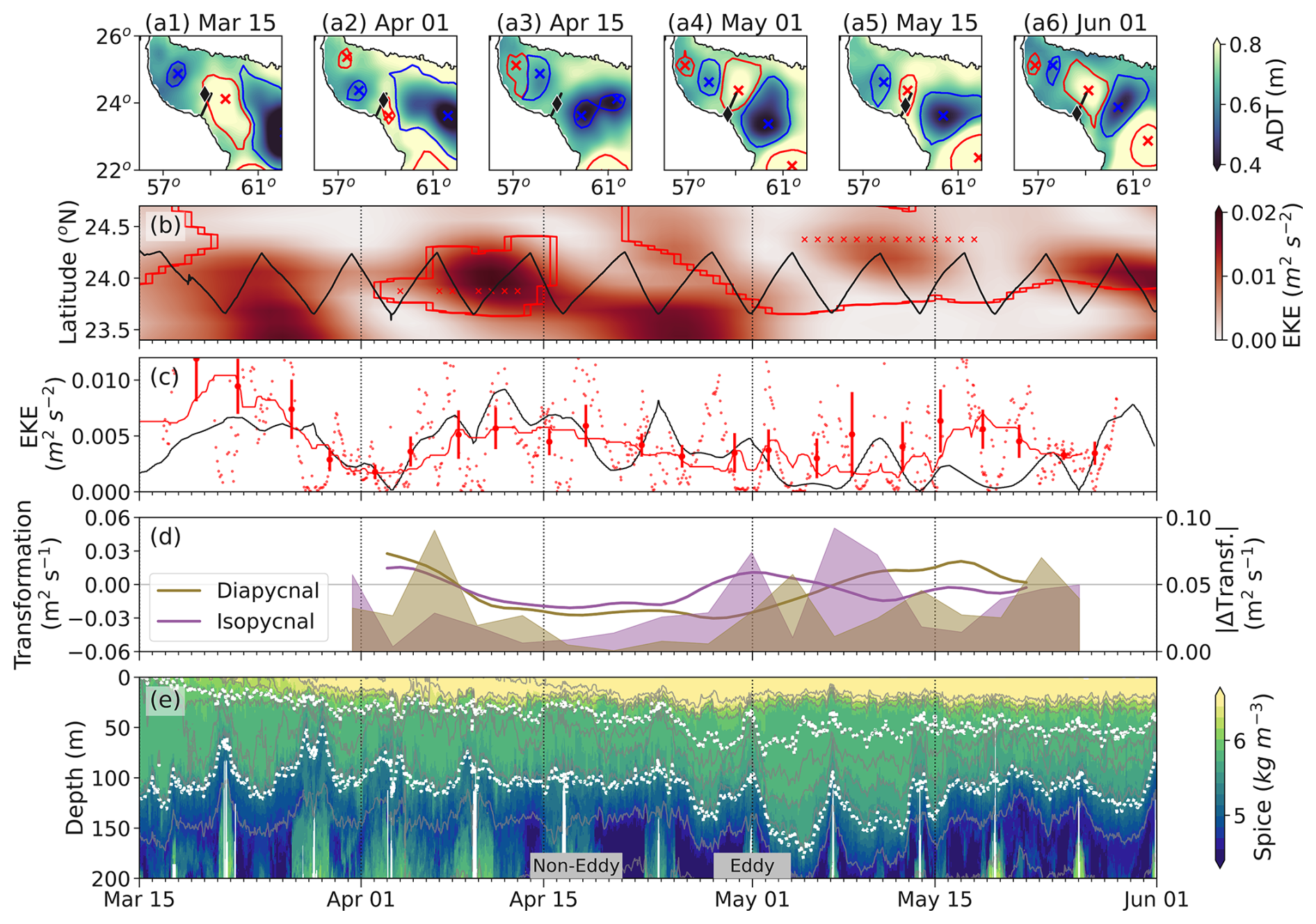
Figure 5 Mesoscale eddies and mode water transformation. (a1–a6) Snapshots of Absolute Dynamic Topography (ADT) in the Sea of Oman on the 1st and 15th day of each month between March and June. The glider location on each date is marked with a black diamond, and its transect is shown as a black line. The eddies are retrieved from TOEddies Atlas (anticyclones in red, cyclones in blue): the eddy center (×) and the maximum extent (solid contour) are also shown. (b) Hovmoller of EKE from satellite-derived geostrophic velocities with the glider track in black. The eddy center (×) and the contours of maximum extent (solid contour) are shown as in panel (a). (c) EKE retrieved from the glider dive-average current (small red dots), after applying a 24 h rolling mean (red line), and average per transect (large red dots) with the standard deviation for the transect as a vertical red line. EKE retrieved from ADT (black line), scaled by a factor of 2 to match the magnitude of the EKE from the glider. (d) Mean transformation per transect (left axis), and the absolute change of transformation over time ($\left|\mathrm{\Delta }\text{Transf.}\right|$; right axis) to show when the change in transformation occurs for both diapycnal and isopycnal transformation. (e) Spice time series with the top and bottom boundaries of the core of the mode water (25–25.25 kg m⁻³; white dotted lines) and isopycnals (gray lines). The two labels show the periods chosen as “Eddy” and “Non-Eddy” study cases in Fig. 6.

The glider-derived observations reveal the vertical imprint of these eddies on the thermohaline structure and associated water mass transformation. The observed vertical displacements of isopycnals and intrusions of anomalous water masses (Fig. 5e) are consistent with mesoscale stirring. These anomalies coincide with changes in isopycnal and diapycnal transformation along with mesoscale eddy activity (Fig. 5d), suggesting an active role of mesoscale dynamics in modulating vertical exchanges and interior ventilation. For instance, around 6 April, when an anticyclone is present, a marked increase in surface EKE (Fig. 5b) corresponds with simultaneous peaks in both isopycnal and diapycnal transformation rates of change ($\left|\mathrm{\Delta }\text{Transf.}\right|$, Fig. 5c and d), suggesting intensified stirring and mixing as the glider samples through the eddy structure.

Around 15 April (non-eddy case), the mesoscale eddy moves away from the glider transect, as indicated by both the ADT maps (Fig. 5a3) and the glider spice time series, where isopycnals flatten (Fig. 5e). The glider trajectory during this period does not intersect any prominent eddy (Fig. 5b), suggesting that it is transiting through a relatively quiescent background flow. Correspondingly, the transformation rates, both diapycnal and isopycnal, are stable and similar to the ones derived from the climatology (negative and O(10⁻²), Figs. 3f and 5d). This calm period contrasts with the more dynamic intervals before and after, suggesting that enhanced transformation is closely tied to eddy presence and activity. The transformation around 15 April thus serves as an ad hoc baseline, highlighting the mesoscale-driven nature of the stronger exchange events observed throughout the record.

A second event occurs around 27 April–3 May (Eddy case), when the glider crosses an anticyclone again (Fig. 5a4, b, and e) and isopycnal transformation increases (Fig. 5d), underscoring the dominant role of mesoscale processes in lateral tracer transport. This is followed by a pronounced diapycnal transformation event, likely driven by vertical exchanges at eddy boundaries and/or interaction with shelf bathymetry.

Figure 6 Case studies. (a) Mean diapycnal and (b) isopycnal transformations in geographical space (distance from shelf vs. depth). Gray lines: isopycnals; red lines: 25.00 and 25.25 kg m⁻³; dotted: iso-spice. Density classes lighter than 24.5 kg m⁻³ are diagonally hatched (//) to exclude water classes with a potential air-sea flux transformation term. (c) Diapycnal, isopycnal transformations, and exchange fluxes averaged over 0.25 kg m⁻³ density bands. Panels (d)–(f) show a case without an eddy (Non-Eddy Case); (g)–(i) a case with an eddy (Eddy Case). (d, g) Diapycnal, (e, h) isopycnal transformations in geographical space; (f, i) transformations and fluxes in density space. In (d)–(e), (g)–(h), dotted and solid isopycnals correspond to initial and final time steps. Vertical hatches ($\left|\right|$) mark regions where exchange flux accounts for >25 % of volume change. Density classes lighter than 24.5 kg m⁻³ are hatched (//) to exclude water classes with a potential air-sea flux transformation term. (j–l) Spice-integrated averages of (j) diapycnal, (k) isopycnal transformations, (l) exchange flux; lines: eddy (solid), non-eddy (dashed), and Argo climatology (dotted). The averages are on the absolute values of the transformations, thus focusing on their magnitudes rather than their direction. (m) Mean density profile for eddy (solid) and non-eddy (dashed) classification, and climatology (dotted). N indicates the number of glider sections that contribute to the mean. Lines in (c), (f), and (i)–(l) separate 0.25 kg m⁻³ bands; red lines denote the potential density range of mode water (25 and 25.25 kg m⁻³). Note differing x axis ranges in (c, f, i), and (j–l).

To investigate the spatial structure of water-mass transformation and its dependence on mesoscale eddy activity, we remapped the transformations in distance-pressure coordinates from the shelf. The transformation rates, when averaged over the repeated sections of the entire glider deployment (Fig. 6a and b) show weak diapycnal and isopycnal transformations. This mean view closely resembles those derived from the monthly climatological dataset, despite the climatology being composed of basin-wide Argo profiles (Fig. 3b), reaffirming that glider-based observations can reproduce the climatological view when averaged over long enough timescales, and that high-frequency variability is largely smoothed out in monthly means.

We compare the average transformation sections with two contrasting case studies: one with no eddy presence (Fig. 6d–f) and one with an eddy (Fig. 6g–i, the periods marked in Fig. 5e). The Non-Eddy Case (Fig. 6d–f) provides a baseline scenario where the glider transect occurs in a region with no identifiable eddy, as confirmed by the lack of coherent structures in the ADT maps (Fig. 5a3). Both isopycnal and diapycnal transformation rates are comparable to the climatological mean and are relatively weak within the mode water core ($\sim -\mathrm{0.01}$ and 0.005 m² s⁻¹, respectively, Figs. 3, 6d and e).

The Eddy case (Fig. 6g–i) captures a glider transect through an anticyclonic eddy. In contrast to the quiescent background conditions seen in the Non-Eddy Case, this eddy drives an order of magnitude enhancement of diapycnal transformation above and below the mode water core ($\sim \mathrm{0.05}{\mathrm{m}}^{\mathrm{2}}{\mathrm{s}}^{-\mathrm{1}}$), pointing to intense vertical exchanges associated with eddy-induced mixing. Isopycnal transformation is also intensified and spatially coherent along sloping density surfaces ($\sim \mathrm{0.04}{\mathrm{m}}^{\mathrm{2}}{\mathrm{s}}^{-\mathrm{1}}$). The elevated isopycnal transformation rates imply vigorous lateral mixing along density surfaces, enhanced by eddy-driven stirring and frontal slumping. Such strong transformation rates suggest that the eddy acts as an efficient conduit for water-mass transformation, especially within mode water density layers. This case highlights the dynamically active role of anticyclonic eddies in modulating both vertical and lateral mixing processes, and thus promoting the redistribution of heat and salt and contributing to the ventilation of the ocean interior.

The exchange term (grey bars in Fig. 6c, f, and i), calculated as the residual in the transformation budget, serves as a proxy for advective fluxes through the section and can highlight dynamically active regions where advection dominates over mixing. In the Eddy Case, this term is particularly pronounced, indicating a strong advective component related to eddy presence ($\mathrm{0.59}\pm \mathrm{0.48}{\mathrm{m}}^{\mathrm{2}}{\mathrm{s}}^{-\mathrm{1}}$, Fig. 6i). In contrast, the exchange flux is much weaker in both the mean section and the Non-Eddy Case ($\mathrm{0.16}\pm \mathrm{0.13}{\mathrm{m}}^{\mathrm{2}}{\mathrm{s}}^{-\mathrm{1}}$, Fig. 6c and f), suggesting a reduced role of advective processes. Eddies, both surface and subsurface, are well known to transport coherent parcels across long distances (e.g., Frenger et al., 2018), driving the strong exchange seen here. Altogether, the exchange term adds an important dimension to the volume budget, helping to quantify the net effect of non-mixing processes, and further supporting the view that mesoscale advection can be a dominant pathway for ventilation and altering stratification in the upper ocean.

The impact of the dynamical regime on transformation magnitudes within the mode water layer is striking (Fig. 6j–l). The passage of mesoscale eddies leads to a marked intensification of all three components of the volume budget within the mode water layer, reflecting enhanced isopycnal and diapycnal mixing as well as increased advective exchange (see summary schematic in Fig. 2). Compared to non-eddy conditions, diapycnal, isopycnal, and exchange fluxes increase by 61 %, 45 %, and 66 %, respectively (Fig. 6j–l). In the absence of eddies, mode water undergoes significantly weaker transformation – with transformation magnitudes similar to the climatological average (Fig. 6j–l). It is noteworthy that these estimates represent integrated values across the glider transect, and local transformation rates may vary substantially, enhanced or suppressed, depending on eddy position, intensity, and interactions with topography.

To further contextualize these differences, we compared the transformation rates under eddy and non-eddy conditions with the climatological mean derived from Argo profiles. Diapycnal transformation exhibits the largest relative increase during eddy periods, rising by 163 % compared to the climatological mean (Fig. 6j). This substantial enhancement likely reflects intensified vertical exchange driven by eddy-related processes that are absent from monthly climatologies. Even outside of eddy influence, the diapycnal transformation from the glider data remains elevated ($\sim \mathrm{0.13}{\mathrm{m}}^{\mathrm{2}}{\mathrm{s}}^{-\mathrm{1}}$, a 63 % increase relative to the climatological mean), likely due to the glider's ability to resolve finer-scale vertical structure and fluxes resulting from diapycnal mixing.

Isopycnal transformation also increases under eddy influence, with a pronounced peak in the mode water layer ($\sim \mathrm{0.16}{\mathrm{m}}^{\mathrm{2}}{\mathrm{s}}^{-\mathrm{1}}$), corresponding to a 43 % rise over the climatological mean (Fig. 6k). This points to enhanced lateral stirring and strain-driven intrusions along density surfaces, characteristic of mesoscale eddy activity. In contrast, during non-eddy conditions, isopycnal transformation remains weaker and closely matches the climatological estimate ($\sim \mathrm{0.11}{\mathrm{m}}^{\mathrm{2}}{\mathrm{s}}^{-\mathrm{1}}$). This suggests that eddy-related strain and intrusions play a major role in redistributing water masses and altering thermohaline structure within the mode water. In the absence of eddies, isopycnal transformation is reduced and comparable to the climatological mean.

The exchange component (Fig. 6l) similarly shows a pronounced peak in the presence of eddies ($\sim \mathrm{0.5}{\mathrm{m}}^{\mathrm{2}}{\mathrm{s}}^{-\mathrm{1}}$, 140 % increase relative to climatology), and is notably lower under non-eddy conditions ($\sim \mathrm{0.3}{\mathrm{m}}^{\mathrm{2}}{\mathrm{s}}^{-\mathrm{1}}$, 45 % above the climatological mean). The greater exchange fluxes observed in the high-resolution glider dataset reflect the contribution of strong mesoscale advection not captured in the monthly climatologies.

4 Discussion

Mode waters play a crucial role as pathways connecting the surface and subsurface ocean, influencing the distribution and transport of tracers, including heat, salt, oxygen, and other biogeochemical properties. For instance, in the Arabian Sea, mode waters bound the upper oxycline of the Arabian Sea oxygen minimum zone, thus playing a central role in shaping regional oxygen distributions (Font et al., 2025). As shown by Jutras et al. (2025), at long-term and large spatial scales, more than 50 % of oxygen changes along mode water ventilation pathways can be attributed to mixing with surrounding oxygen-poorer waters. While we do not diagnose oxygen directly, our results extend this understanding by showing that the physical drivers of such mixing are strongly intensified at short timescales during eddy activity. These episodic but vigorous transformation events likely modulate ventilation efficiency and tracer redistribution within mode waters.

High-resolution glider observations reveal the much greater intermittency and intensity of transformation processes missed in climatological datasets. This challenges the underlying assumptions of climatological approaches for estimating water mass transformation and understanding upper-ocean dynamics. Monthly climatologies, while valuable for capturing broad seasonal trends, inherently smooth out the episodic and spatially localized processes (e.g., mesoscale eddies and submesoscale fronts) that strongly contribute to net water-mass transformation. Our analysis shows that a significant fraction of the total transformation, particularly within the mode water layer, occurs during short-lived eddy events, which are effectively diluted in monthly-averaged fields (Figs. 3 and 4). As a result, climatological approaches miss sub-monthly variability and underestimate both the intensity and variability of transformation processes (Fig. 4), particularly the contributions from isopycnal stirring and advective exchange (Fig. 6).

Mesoscale eddies can trap and transport mode water, preserving its properties and prolonging the lifespan of this buffer layer. In the Arabian Sea, eddies have been shown to modulate the distribution and characteristics of water masses such as the Arabian Sea High Salinity Water (Thoppil, 2024; Trott et al., 2019). Moreover, anticyclonic eddies have been found to trap more mode water than cyclonic ones (e.g., Liu and Li, 2013, in the North Atlantic), contributing significantly to total mode water transport – up to 17 % south of the Kuroshio Extension (Shi et al., 2018), comparable to the transport by the mean flow (Xu et al., 2016). We complement these findings by showing that, at short spatial and temporal scales, eddies transform mode waters (Figs. 2, 5, and 6). We hypothesize that by driving intermittent but intense exchanges, eddies can influence stratification and shape mode water transformation. While the water-mass transformation framework allows for indirect estimation of the integrated effects of mixing, understanding the specific mechanisms behind these transformations, particularly at fine scales, requires direct observations. Including turbulence measurements, such as microstructure-derived diffusivities to resolve the role of vertical mixing, could allow for disentangling those from lateral stirring and advection, and thus refine the interpretation of transformation processes in dynamic regions like the Sea of Oman.

Mesoscale eddies play a crucial role as biogeochemical agents. Subsurface eddies can carry oxygen and nutrient signatures over distances of hundreds of kilometers (Frenger et al., 2018) and can influence subsurface biogeochemistry over extended periods (Karstensen et al., 2017; Schütte et al., 2016). Mesoscale eddies influence the boundaries of oxygen minimum zones (e.g., Auger et al., 2021; Eddebar et al., 2021; Sarma and Udaya Bhaskar, 2018), and it has been shown that eddy-resolving models lead to better representation of these zones' intensity and extent (Calil, 2023; Lévy et al., 2022; Resplandy et al., 2012). The intensified isopycnal and exchange-driven transformations we observe during eddy periods (Figs. 2, 5, and 6) imply stronger horizontal and vertical transport, reinforcing the idea that they play a disproportionate role in regulating fluxes of heat, salt, and biogeochemical tracers in the upper ocean.

We suggest that ventilation timescales for the mode water layer are highly variable in time and space. This variability has significant implications for interpreting biogeochemical observations or budgets derived from time-averaged or coarse-resolution data, which may underestimate the influence of short-lived but intense eddy events. Our findings raise important questions about the timescales over which biological activity and physical mixing interact and balance across broader spatial and temporal domains, which need to be further investigated. Capturing this level of detail is essential for improving biogeochemical model parameterizations, which rely on an accurate representation of exchange rates and timescales. Moreover, it provides a basis for evaluating how these processes may respond to future changes in ocean stratification, eddy activity, and circulation patterns.

5 Conclusions

Through a detailed characterization of the temporal variability, we find that the mode water core in the Sea of Oman becomes progressively denser and mintier as its volume diminishes between March (when it is capped just below the surface) and June. By applying the water mass transformation framework in σ-τ space to both high-resolution glider data and a monthly climatological Argo dataset, we quantify the dominant timescales and transformation processes acting within the mode water layer. Isopycnal transformation rates were, on average, three times greater than diapycnal transformation. However, episodic mesoscale eddy events lead to locally enhanced diapycnal fluxes.

This framework, traditionally applied to coarse-resolution climatologies or model simulations, proves capable of capturing transformation variability and extremes that are absent from monthly climatological datasets, highlighting the unique value of gliders. We estimate that the likelihood of recovering the 3 d sampled mean from monthly climatologies is between 40 %–60 %, emphasizing how coarse temporal sampling can distort our understanding of the inherently episodic and dynamic nature of water-mass transformation. This observed variability is attributed to mesoscale eddies.

During eddy passages, all three components of the mode water volume budget-diapycnal, isopycnal transformations, and exchange flux – are significantly intensified compared to non-eddy conditions (as the schematic in Fig. 2 shows). Overall, our results demonstrate that transformation within the mode water layer is strongly enhanced by mesoscale activity. These findings underscore the need for sustained, high-resolution observations, as they would allow us to link integrated transformation rates more explicitly to underlying physical drivers, resolve the vertical structure of mixing processes, and assess the role of mesoscale and submesoscale dynamics and topographic interactions. Ultimately, combining transformation diagnostics with targeted in situ measurements will improve our ability to constrain ocean ventilation and tracer budgets, refine model parameterizations, and evaluate how these processes respond to a changing climate.