Multi-year predictability of hydrography and circulation on the U.S. Northeast Shelf: a dynamical downscaling perspective

The U.S. Northeast Shelf (NES) is a dynamic and economically important marine ecosystem where temperature and salinity variability are shaped by interactions among large-scale climate variability, Gulf Stream shifts, mesoscale eddies, and local shelf processes. Predicting these variations on multi-year timescales remains a major challenge for current climate systems, as global models at typically 1–2° resolution exhibit poor skills for the NES. Here, we evaluate a high-resolution regional prediction of NES based on the downscaling of global Community Earth System Model Decadal Prediction Large Ensemble (CESM-DPLE) using the Regional Ocean Modeling System (ROMS-DOWN) to assess its potential for improving interannual-to-decadal prediction skill on the NES. Compared to CESM-DPLE, ROMS-DOWN substantially reduces mean-state biases in temperature, salinity, sea surface height, and upper-ocean heat content across the shelf and slope, where bathymetry effect and shelf-slope exchange are critical but poorly resolved in global models. Both deterministic and probabilistic metrics indicate improved forecast performance with lead time up to 5 years. The predictive skill reflects contributions from externally forced trends and interannual-to-decadal internal variability, with dominant timescales of predictability differing among variables. ROMS-DOWN also skillfully reproduces key shelf features such as the Middle Atlantic Bight cold pool and slope-water mixing characteristics in the Gulf of Maine, though their predictability remains moderate likely due to internal variability, boundary condition biases, and model uncertainties. Overall, these results demonstrate that dynamical downscaling can effectively bridge large-scale climate predictability and regional coastal processes, providing a foundation for improved multi-year prediction and understanding of ocean variability on the NES.

1 Introduction

The U.S. Northeast Shelf (NES) Large Marine Ecosystem is one of the most dynamic and socioeconomically important marine systems in the world, supporting valuable fisheries and coastal communities (Link et al., 2002; Lucey and Nye, 2010; Gartland et al., 2023). Over recent decades, the NES has experienced substantial changes in its hydrography, circulation, and ecosystem structure in response to natural climate variability and anthropogenic forcing (Claret et al., 2018; Chen et al., 2020; Gonçalves Neto et al., 2021; Guo et al., 2022a; Friedland et al., 2024). These physical changes strongly influence biological productivity and fish distributions, creating challenges for resource management and climate adaptation (Pershing et al., 2015; McHenry et al., 2019; Friedland et al., 2025). Developing reliable predictions of the physical environment on seasonal to multi-year timescales is therefore a critical step toward supporting climate-informed fisheries management and improving ecosystem forecasts for the NES.

Skillful predictions for the NES is challenging due to the region's complex dynamics and multi-scale processes. The NES lies at the confluence zone of contrasting subpolar and subtropical water masses, where cold, fresh waters advected southward by the Labrador Current meet warm, saline waters carried northward by the Gulf Stream and slope currents (Loder, 1998; Chapman and Beardsley, 1989; Fratantoni and Pickart, 2007; Kwon et al., 2010). This intersection, together with strong interactions between the shelf and open ocean through multiscale dynamic processes and frequent atmospheric disturbances along the mid-latitude storm track, drives large variability on timescales from subseasonal to decadal (Kelly et al., 2010; Chen et al., 2014a; Guo et al., 2023). Standard-resolution global prediction models with 1° horizontal resolution struggle to capture these variabilities because they poorly resolve Gulf Stream mean position and variability, shelf–slope exchange, coastal currents, and fine-scale bathymetry, all of which are critical to reproducing NES water characteristics and their variability (e.g., Saba et al., 2016; Jacox et al., 2020; Chen et al., 2022).

At the same time, observational and modeling studies suggest that variations in water properties on the NES may be influenced by predictable large-scale signals. Variability in the North Atlantic Oscillation (NAO), Atlantic Meridional Overturning Circulation (AMOC), and Gulf Stream path have all been linked to temperature and salinity changes on the NES with time lags of 1–5 years (Mountain, 2012; Xu et al., 2015; Saba et al., 2016; Gonçalves Neto et al., 2021; Karmalkar and Horton, 2021). For instance, Labrador Slope Water intrusions into the Gulf of Maine are correlated with AMOC variability 1 to 2 years earlier (Saba et al., 2016), while Gulf Stream path shifts have been shown to modulate shelf temperature and fish distributions (Nye et al., 2011; Davis et al., 2017; Gonçalves Neto et al., 2021). This implies that multi-year predictability over the NES may be achievable if large-scale oceanic and/or atmospheric signals are effectively transmitted to the coastal environment through enhanced model resolution and better representation of local dynamics.

Recent advances in global climate prediction systems have demonstrated that skillful forecasts on seasonal to decadal timescales are increasingly achievable, particularly in regions where large-scale ocean dynamics provide memory to the climate system (Meehl et al., 2009; Yeager et al., 2018; Christensen et al., 2020; Yeager et al., 2022). In the North Atlantic, initialized decadal prediction systems – including the CESM Decadal Prediction Large Ensemble (CESM-DPLE) – have shown notable skill in predicting variability in the subpolar gyre, AMOC, Labrador Sea convection, and basin-scale SST patterns several years in advance (Yeager et al., 2018; Athanasiadis et al., 2020). These forecasts capture coherent low-frequency ocean signals linked to heat content anomalies, buoyancy forcing, and large-scale circulation changes, underscoring the potential for predictable pathways that can influence downstream regions such as the NES. The demonstrated skill of CESM-DPLE in the broader North Atlantic provides a strong foundation for regional downscaling: if large-scale predictable signals are reproduced in the global system, a high-resolution regional model may translate that information into improved predictability of coastal ocean properties.

Building on these advances in large-scale prediction, dynamical downscaling provides a pathway to bridge large-scale climate signals with regional-scale ocean processes by embedding a high-resolution regional model within global forecast systems. Previous downscaling studies have demonstrated substantial improvement in the representation of NES hydrography using dynamical downscaling at both seasonal (Ross et al., 2024) and decadal timescales (Koul et al., 2024). However, these approaches target distinct prediction horizons, and the extent to which dynamical downscaling enhances forecast skill on intermediate (multi-year) timescales remains less well understood. This timescale is particularly relevant for living marine resource management, where decisions often require outlooks beyond seasonal forecasts and are more actionable than decadal projections.

In this study, we evaluate the improvement in multi-year prediction skill over the NES using a high-resolution Regional Ocean Modeling System (ROMS) configuration (hereafter ROMS-DOWN) forced by large-scale anomaly fields from CESM-DPLE (Yeager et al., 2018). Although the ROMS model domain extends beyond the shelf to include the adjacent Slope Sea and Gulf Stream, our evaluation focuses primarily on prediction skill over the NES. By quantifying the improvements and limitations of dynamical downscaling, we aim to achieve a better understanding of multi-year predictability on the NES and to provide guidance for advancing climate-informed ocean forecasting and ecosystem management in the region.

2 Data and Methods

2.1 Observations and reanalysis

Two satellite-based observational datasets are used to evaluate mean-state fidelity of both the reanalysis dataset and the model outputs on the NES: one for sea surface temperature (SST) and the other for sea surface height (SSH). For SST, we use the NOAA Optimum Interpolation Sea Surface Temperature (OISST; Reynolds et al., 2007; Huang et al., 2021), which provides high-resolution daily fields based on blended satellite and in situ observations. For SSH, we use the AVISO (Archiving, Validation, and Interpretation of Satellite Oceanographic) gridded altimetry product archived from the data portal Copernicus Marine Environment Monitoring Service (CMEMS), which merges measurements from multiple satellite missions to generate consistent maps of sea level anomalies relative to a long-term mean. Both datasets are provided at a horizontal resolution of approximately 25 km and are used exclusively to validate the climatological mean distributions across the model domain, thereby providing a reference for the mean pattern of ocean circulation and surface water properties on the NES.

To evaluate multi-year prediction skill, we employ the GLORYS ocean reanalysis (Global Ocean Reanalysis and Simulation) version 12V1, produced by Mercator Ocean and distributed through the CMEMS (Lellouche et al., 2021). The CMEMS product is provided on a regular $\mathrm{1}/\mathrm{12}$° (∼ 8 km in the study area) grid with 50 standard vertical levels and spans the satellite altimetry era from 1993 to the present (Lellouche et al., 2021). It assimilates a wide range of observations, including satellite-derived SST and SSH, sea-ice concentration, and in situ profiles of temperature and salinity from ARGO floats, and ship-based measurements. Independent evaluations have shown, through comprehensive comparisons with available observations, that GLORYS is one of the best global reanalysis products in representing the climatological hydrography, circulation, and their temporal and spatial variability over the NES region (Castillo-Trujillo et al., 2023). These characteristics make GLORYS an appropriate benchmark for assessing the predictive skill of both the regional and global prediction systems analyzed in this study. One limitation of GLORYS is that it does not explicitly include tidal forcing, which can contribute to residual temperature and salinity biases in strongly tidal regions such as Georges Bank and parts of the Gulf of Maine (Castillo-Trujillo et al., 2023). However, in this study prediction skill is evaluated using annual-mean anomalies with a lead-time-dependent climatology removed, which reduces sensitivity to mean-state biases and high-frequency variability associated with tidal processes. In addition, GLORYS's representation of shallow coastal waters is limited, which may introduce additional uncertainties in nearshore regions.

2.2 CESM Decadal Prediction Large Ensemble (CESM-DPLE)

The global simulations used in this study are based on the Community Earth System Model version 1.1 (CESM1.1), a fully coupled global climate model that integrates atmosphere, ocean, sea ice, and land components through a central flux coupler (Hurrell et al., 2013). The atmospheric component employs the Community Atmosphere Model version 5 (CAM5) at approximately 1° × 1° horizontal resolution with 30 vertical levels (Park et al., 2014), while the ocean component uses the Parallel Ocean Program version 2 (POP2) at a comparable 1° × 1° resolution with 60 vertical levels (Smith et al., 2010). Sea ice is simulated with the Community Ice Code version 4 (CICE4) on the ocean grid (Hunke et al., 2010), and land processes are represented by Community Land Model version 4 (CLM4) on the atmospheric grid (Lawrence et al., 2011).

To provide large-scale lateral boundary condition and surface forcing fields as well as the initial condition for the dynamic downscaling experiments, and to compare skill directly with a global prediction system, we use the CESM Decadal Prediction Large Ensemble (CESM-DPLE; Yeager et al., 2018). CESM-DPLE is a global prediction system, which consists of 40 ensemble members, each initialized every 1 November from 1954 to 2015, and integrated for 10 years. The system uses CESM1.1 with nominal 1° horizontal resolution in both the ocean and atmosphere. Initialization of the ocean and sea ice is based on an ocean–sea ice-only simulation forced with Coordinated Ocean Research Experiments (CORE) bulk fluxes (Danabasoglu et al., 2016), while the atmosphere and land components are initialized from the CESM Large Ensemble (CESM-LE; Kay et al., 2015). The external forcing is prescribed to be identical to CESM-LE.

CESM-LE is a fully coupled companion ensemble of simulations designed to represent the response of the climate system to external forcing (e.g., greenhouse gases, aerosols, volcanic eruptions) in the absence of initialization from observations. Each member is generated by applying small perturbations to the atmospheric initial state. Because CESM-LE is uninitialized, each member exhibits year-to-year ocean internal variability such that the temporal evolution is not necessarily consistent with observations. Instead, the ensemble mean captures the externally forced component of variability. As such, CESM-LE serves two important roles in this work: (1) it provides a baseline for assessing how much of the forecast skill in CESM-DPLE and ROMS-DOWN arises from external forcing versus initialization, and (2) it illustrates the level of multi-year predictability expected solely from forced long-term trends or externally driven decadal variations.

CESM-DPLE has been widely used to assess decadal predictability of the Atlantic and global climate system, and has demonstrated robust skill in the subpolar North Atlantic (Yeager et al., 2018; Athanasiadis et al., 2020). In CESM-DPLE, high-frequency atmospheric output (daily or sub-daily) is archived for only a subset of ensemble members; the implications of this constraint for the regional downscaling design are described in Sect. 2.4.

2.3 ROMS Hindcast (ROMS-HIND)

To evaluate the performance of our regional ocean model configuration, we use a hindcast simulation (ROMS-HIND). ROMS-HIND is based on the Regional Ocean Modeling System (ROMS), a free-surface hydrostatic, primitive equations numerical model (Shchepetkin and McWilliams, 2005). The model domain encompasses the NES, adjacent slope waters and the Gulf Stream. It extends from 30 to 55° N and from 80 to 35° W (Fig. 1). The northern boundary of ROMS-HIND and ROMS-DOWN is set within the subpolar gyre so that the boundary condition from CESM-DPLE may contain highly skillful prediction (Yeager et al., 2018). The model has a curvilinear grid with a ∼ 5 km spatial resolution and 40 terrain-following vertical levels that are unevenly spaced with a higher resolution near the surface. A minimum depth of 10 m was imposed by modifying the bathymetry prior to the simulation to avoid wetting and drying of grid cells. At the open boundaries, Chapman boundary conditions were used for the free surface, Shchepetkin lateral boundary conditions for the depth-averaged momentum, and all other fields use radiation boundary conditions (Chapman, 1985; Mason et al., 2010).

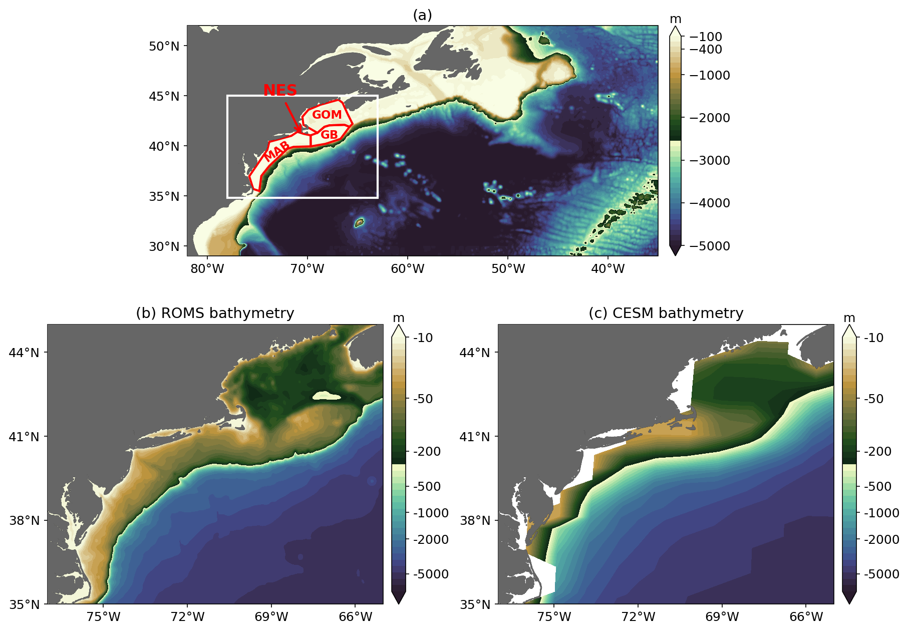
Figure 1 Study area. (a) ROMS model domain showing bathymetry. The white box denotes the analysis region shown in (b). (b) Bathymetry within the analysis region. The U.S. Northeast Shelf (NES) is defined as the shelf region shallower than 200 m and consists of the Middle Atlantic Bight (MAB), Georges Bank (GB), and the Gulf of Maine (GOM), outlined in red. (c) Same as (b), but for the CESM bathymetry.

The model bathymetry is derived from the ETOPO1 Global Relief Model (Fig. 1a and b). To reduce the pressure gradient errors due to the steep bathymetry, the bathymetry was smoothed with the Batteen and Miller (2009) method using a maximum roughness value of R_xo = 0.25 and R_x1 = 7. Several sensitivity experiments were conducted in which R_xo was varied, producing different degrees of bathymetry smoothing and shifts in the shelf break position relative to the coast (Fig. A1 in the Appendix). The configuration presented here was selected because it yielded the most realistic Gulf Stream path – including separation near Cape Hatteras – while minimizing pressure gradient errors and maintaining a realistic shelf circulation.

Surface atmospheric forcing is obtained from the European Centre for Medium-Range Weather Forecasts (ECMWF) Reanalysis v5 (ERA5) (Hersbach et al., 2020). The ERA5 analysis provides hourly estimates for a large number of atmospheric, ocean-wave, and land-surface quantities. ERA5 combines vast amounts of historical observations into global estimates using advanced modeling and data assimilation systems. ROMS-HIND is forced with hourly data including zonal and meridional wind, shortwave and longwave radiation, cloud, atmospheric pressure, rain, and humidity via COARE 3.5 bulk flux formula (Edson et al., 2013). The initial and open boundary ocean conditions are produced from daily $\mathrm{1}/\mathrm{12}$° GLORYS12v1 output. The model is forced with monthly climatological river discharge and temperature at 21 river mouths along the NES, derived from the global river reanalysis dataset of Dai (2021). Tidal forcing is included in the model using the dominant semidiurnal tidal constituents (M2 and S2) from the TPXO09 global tidal model (Egbert and Erofeeva, 2002), providing the primary tidal mixing necessary to realistically represent the circulation over the Shelf (Chen and He, 2015). The simulation was performed from January 2004 to December 2010 which overlaps with the satellite and reanalysis datasets used for validation and with the ROMS-DOWN predictions described below.

2.4 ROMS Downscaling (ROMS-DOWN)

To perform dynamical downscaling for multi-year prediction on the NES, we employ a regional forecast system (ROMS-DOWN) based on the same ROMS configuration used in ROMS-HIND. Unlike ROMS-HIND, which is initialized and forced solely by reanalysis products, ROMS-DOWN is initialized and forced by anomalies from CESM-DPLE. The atmospheric forcing is constructed as the 1993–2024 ERA5 monthly climatology plus daily CESM-DPLE anomaly fields, where the daily anomalies are computed relative to a daily climatology obtained by interpolating the 1993–2010 monthly climatology. Similarly, the ocean initial and lateral boundary conditions are constructed from the 1993–2021 GLORYS monthly climatology plus monthly CESM-DPLE ocean anomaly fields computed relative to the 1993–2010 monthly climatology. The different climatology periods reflect the temporal coverage of the respective datasets. Monthly ocean anomalies are used because the CESM-DPLE ocean variables required to force the regional model are available only as monthly means. This temporal resolution is also appropriate because the large-scale ocean variability relevant to multi-year prediction evolves primarily on monthly to longer timescales, while also reducing computational and storage requirements. River input is prescribed identically to ROMS-HIND using monthly climatological river transport and temperature at 21 river mouths along the NES. Because river discharge is prescribed as a repeating climatology, interannual freshwater variability is not included in ROMS-DOWN. This “anomaly downscaling” strategy reduces the impact of mean-state biases in CESM-DPLE while allowing large-scale signals to propagate into the high-resolution regional domain.

ROMS-DOWN consists of 20 start years (1992–2011), each initialized on 1 January with 10 ensemble members and integrated for 8 years, yielding a total of 200 eight-year forecasts. Our downscaling experimental design is constrained by the availability of high-frequency CESM-DPLE atmospheric output. The required daily (or 3-hourly) atmospheric forcing fields are archived only for a limited subset of CESM-DPLE ensemble members and initialization years; as a result, only 10 members provide the necessary forcing for our study period. This output constraint dictated the choice of a 10-member ROMS-DOWN. To assess whether the ensemble size of 10 members and the number of start dates of 20 are sufficient for NES multi-year prediction, sensitivity tests were conducted using the larger CESM-DPLE ensemble set (62 start years and 40 ensemble members). The results suggest that 10 members and 20 start dates are adequate to capture the ensemble-mean forecast signal over the NES region (Fig. A2), indicating that the ensemble design provides a sufficient sample to characterize forecast spread and uncertainty. By construction, ROMS-DOWN preserves the global predictability inherited from CESM-DPLE while resolving smaller-scale shelf processes that are absent in the coarse global simulations (Fig. 1).

To ensure consistent comparisons, all datasets are bilinearly interpolated to the ROMS grid and evaluated using a common land-sea mask. For regional skill assessment (Sect. 2.5), metrics are aggregated over the entire NES, defined here as the combined shelf region encompassing the Gulf of Maine (GOM), Georges Bank (GB), and the Middle Atlantic Bight (MAB), as well as over each subregion individually.

2.5 Skill metrics

We evaluate prediction performance with two deterministic metrics – the Pearson anomaly correlation coefficient (ACC) and the mean square skill score (MSSS) – applied to ensemble-mean annual anomalies, and one probabilistic metric – the Brier Score (BrS) – applied to ensemble probabilities of tercile events following Hervieux et al. (2019). Skill is assessed using the GLORYS ocean reanalysis. To evaluate prediction skill on multi-year timescales, we focus on annual-mean anomalies which emphasizes interannual-to-decadal variability by reducing the influence of seasonal fluctuations. This choice is consistent with the intended application of CESM-DPLE as an annual-to-decadal prediction system. While seasonal analyses may provide additional insight into season-dependent sources of predictability, such analyses are beyond the scope of the present study and will be the subject of future work.

For each variable, we focus on their anomalies based on annual mean and the ensemble mean for each prediction year, which is calculated as:

$$\begin{array}{}\text{(1)}& f_{i\mathit{\tau }}={\displaystyle \frac{\mathrm{1}}{n_{\mathrm{e}}}}\sum _{j=\mathrm{1}}^{n_{\mathrm{e}}}{f}_{ij\mathit{\tau }}.\end{array}$$

where f is the annual mean anomaly, $i=\mathrm{1},\mathrm{\dots },N$ indicates the model initialization years (N=20), $j=\mathrm{1},\mathrm{\dots },n_{\mathrm{e}}$ indicates each ensemble member (n_e = 10), and τ is the prediction lead year (LY1–LY8 in this work). Here, LY1–LY8 denote the first through eighth forecast years following initialization. For example, a forecast initialized on 1 January 1996 has LY1 = 1996, LY2 = 1997,…, and LY8 = 2003. Skill at each lead year is evaluated by pooling all forecasts corresponding to the same lead year across the 20 initialization years.

To evaluate prediction skill, we remove a lead-year-dependent climatology from both the model predictions and the observations. This climatology is computed separately for each prediction lead year by averaging across all initialization years. Removing a lead-year-dependent climatology accounts for systematic forecast drift that develops with increasing lead time and isolates the interannual-to-decadal anomalies used to calculate the skill metrics (Yeager et al., 2018, 2023). Specifically, the anomaly is defined as:

$$\begin{array}{}\text{(2)}& {\widehat{f}}_{i\mathit{\tau }}=f_{i\mathit{\tau }}-{\stackrel{\mathrm{‾}}{f}}_{\mathit{\tau }},{\stackrel{\mathrm{‾}}{f}}_{\mathit{\tau }}={\displaystyle \frac{\mathrm{1}}{N}}\sum _{i=\mathrm{1}}^N{f}_{i\mathit{\tau }},\end{array}$$

Analogously, we sample the observations with 20 initial years and 8 lead years to be parallel to the prediction, with the same observation values repeated for different pairs of initial and lead years, e.g., 1995 observation is used for LY1 of 1995 initialization and LY2 of 1994 initialization. For the observations, o_iτ, ${\widehat{o}}_{i\mathit{\tau }}=o_{i\mathit{\tau }}-{\stackrel{\mathrm{‾}}{o}}_{\mathit{\tau }}$. Because the forecasts are initialized over a finite 20-year period, the verification time windows differ among lead years. For example, LY1 spans 1992–2011, whereas LY8 spans 1999–2018. Consequently, differences in prediction skill among lead years may reflect both dependence on the forecast lead time and differences in the underlying verification periods. The implications of this sampling are discussed further in Sect. 4.

All deterministic skill metrics are computed from $({\widehat{f}}_{i\mathit{\tau }},{\widehat{o}}_{i\mathit{\tau }})$ using the N start-year pairs available at each lead years. For probabilistic metrics, we use the full ensemble to form event probabilities (Sect. 2.5.3) following Hervieux et al. (2019).

2.5.1 Pearson anomaly correlation coefficient (ACC)

ACC measures phase agreement between prediction and observed anomalies:

$$\begin{array}{}\text{(3)}& {\text{ACC}}_{\mathit{\tau }}={\displaystyle \frac{{\sum }_{i=\mathrm{1}}^N{\widehat{f}}_{i\mathit{\tau }}{\widehat{o}}_{i\mathit{\tau }}}{\sqrt{{\sum }_{i=\mathrm{1}}^N{\widehat{f}}_{i\mathit{\tau }}^{\mathrm{2}}}\sqrt{{\sum }_{i=\mathrm{1}}^N{\widehat{o}}_{i\mathit{\tau }}^{\mathrm{2}}}}}.\end{array}$$

Values range from −1 to 1, with positive values indicating that predictions track observed interannual variations.

2.5.2 Mean-square skill score (MSSS)

MSSS quantifies amplitude of error reduction relative to a climatological reference, defined here as the variance of the observed anomalies:

$$\begin{array}{}\text{(4)}& {\text{MSSS}}_{\mathit{\tau }}=\mathrm{1}-{\displaystyle \frac{{\sum }_{i=\mathrm{1}}^N{\left({\widehat{f}}_{i\mathit{\tau }}-{\widehat{o}}_{i\mathit{\tau }}\right)}^{\mathrm{2}}}{{\sum }_{i=\mathrm{1}}^{N{\widehat{o}}_{i\mathit{\tau }}^{\mathrm{2}}}}}.\end{array}$$

Because the denominator equals the observed variance, MSSS>0 denotes improvement over climatology and MSSS<0 degradation. We report MSSS alongside ACC to jointly characterize phase and amplitude bias behavior.

2.5.3 Brier Score for tercile events

Following Hervieux et al. (2019), we assess prediction probability errors using the Brier Score (BrS). For each grid cell, lead year τ, and event definition E (upper or lower tercile of the observed anomaly distribution over the verification period), the ensemble prediction probability for start year i is

$$\begin{array}{}\text{(5)}& f_i={\displaystyle \frac{\mathit{\#}\mathit{\left\{}\text{members\hspace{0.17em}\hspace{0.17em}predicting }E\mathit{\right\}}}{n_{\mathrm{e}}}}\in [\mathrm{0},\mathrm{1}],\end{array}$$

The corresponding observation indicator is defined as $o_i\in \mathit{\{}\mathrm{0},\mathrm{1}\mathit{\}}$, where o_i=1 if the observation for year i falls in the specified event and o_i=0 otherwise. The Brier Score averages the squared probabilistic error:

$$\begin{array}{}\text{(6)}& {\text{BrS}}_{\mathit{\tau }}={\displaystyle \frac{\mathrm{1}}{N}}\sum _{i=\mathrm{1}}^N(f_{i\mathit{\tau }}-o_{i\mathit{\tau }}{)}^{\mathrm{2}}.\end{array}$$

Lower BrS values indicate higher forecast reliability and resolution. Unless noted otherwise, we report BrS separately for upper- and lower-tercile events.

3 Results

3.1 Mean state and variability assessment

To assess how the regional and global prediction systems reproduce the mean spatial structure of key ocean variables on the NES, we show the 2004–2010 time-mean (and ensemble-mean) distributions of SST, SSH, sea surface salinity (SSS), bottom temperature (T_bottom), and 0–200 m heat content (HC_200 m). Observational references are provided by OISST for SST and AVISO for SSH, with GLORYS used for all variables. Note that the GLORYS are compared against OISST and AVISO, while ROMS-HIND, ROMS-DOWN, and CESM-DPLE are compared against GLORYS for the quantification of biases using RMSE (Fig. 2). Spatial maps of the mean bias (model minus GLORYS) for each variable are provided in Fig. A3 to illustrate the spatial structure and sign of these errors. Across all variables, both ROMS-HIND and ROMS-DOWN show markedly improved mean structures and reduced mean biases compared to CESM-DPLE. For SST, CESM-DPLE exhibits a pronounced warm bias on the shelf lacking any sign of shelf break front, with a root-mean-square error (RMSE) of 3.35 °C, primarily due to the overshooting Gulf Stream separation near Cape Hatteras (e.g., Chassignet and Marshall, 2008), whereas ROMS simulations better capture the sharp cross-shelf temperature gradient and Gulf Stream position, with RMSE values below 1.3 °C. SSH patterns reveal that CESM-DPLE overestimates sea level gradient across the shelfbreak (RMSE = 0.22 m), while both ROMS configurations align more closely with AVISO and GLORYS (RMSE ∼ 0.08–0.09 m). Similarly, CESM-DPLE produces overly salty shelf waters (SSS RMSE = 1.89), whereas ROMS-HIND and ROMS-DOWN reproduce the fresher shelf and the offshore gradient (SSS RMSE ∼ 1.3–1.4). Improvements in the regional models are also evident in subsurface variables. For bottom temperature, CESM-DPLE lacks a realistic shelf structure due to its coarse bathymetry and simplified coastlines (Fig. 1), resulting in overly warm and spatially smooth bottom fields (RMSE = 2.22 °C), while the ROMS simulations capture the shelf patterns and the transition to slope waters by more realistically reproducing dynamical constraint imposed by the bottom topography. The 0–200 m heat content (HC_200 m) bias is similarly reduced in the ROMS simulations (RMSE = 1.3–1.9 GJ m⁻²) relative to CESM-DPLE (RMSE = 2.31 GJ m⁻²).

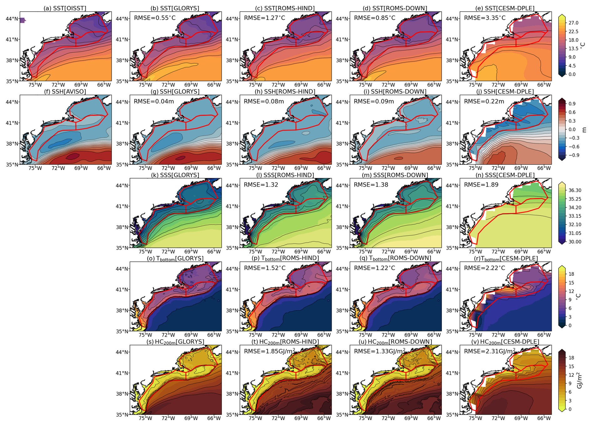
Figure 2 Time-mean (2004–2010) spatial distributions of (a–e) SST, (f–j) SSH, (k–n) SSS, (o–r) T_bottom, and (s–v) HC_200 m from observational products and model simulations. The observational reference is shown in the first column, followed by GLORYS, ROMS-HIND, ROMS-DOWN, and CESM-DPLE. Spatial RMSE values relative to observations for GLORYS or relative to GLORYS for ROMS-HIND, ROMS-DOWN and CESM-DPLE are indicated in the upper-left corner of each panel. For ROMS-DOWN and CESM-DPLE, only lead year 1 (LY1) forecasts overlapping 2004–2010 are used, and results are shown as ensemble means based on 10 and 40 members, respectively. NES and its subregions are outlined in red.

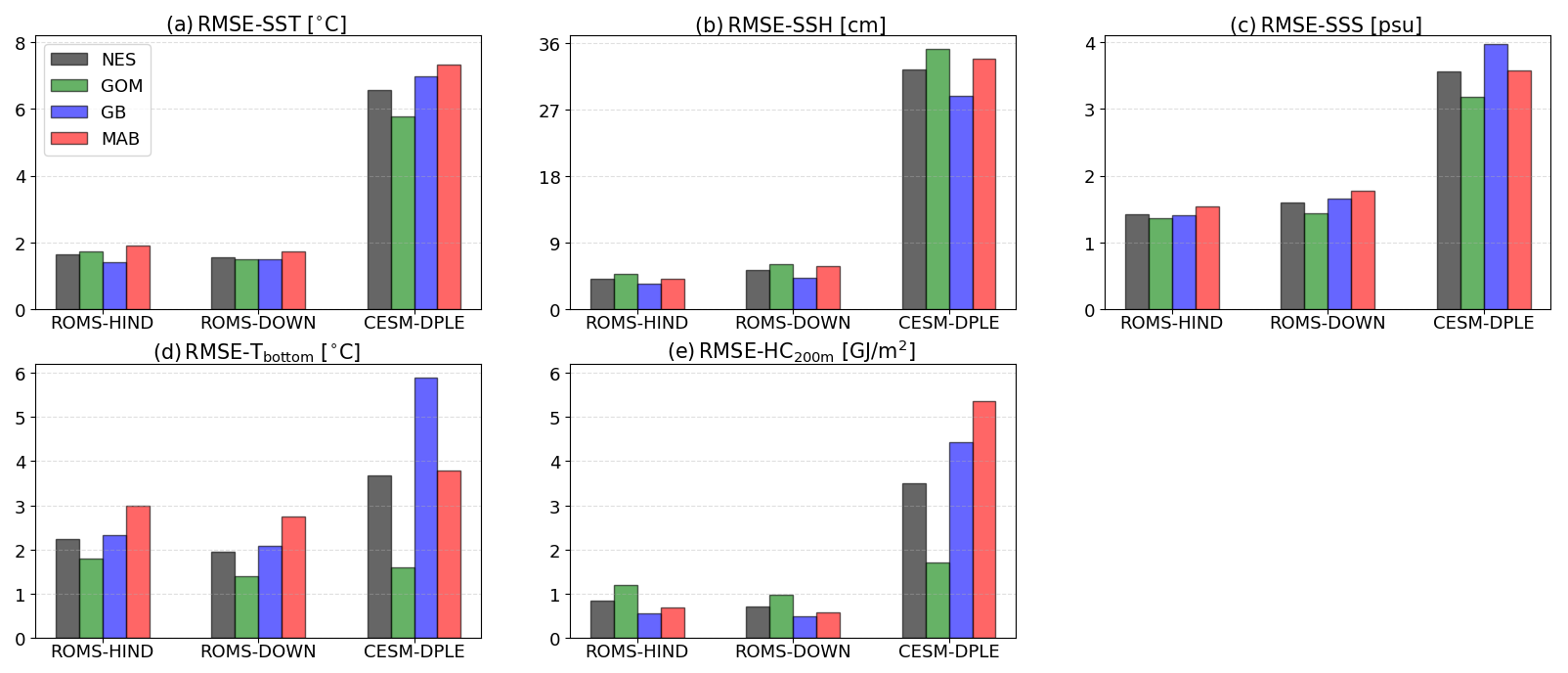
Figure 3 Spatial average of the temporal RMSE (2004–2010; relative to GLORYS) calculated at each grid point within each shelf subregion for (a) SST, (b) SSH, (c) SSS, (d) T_bottom, and (e) HC_200 m in ROMS-HIND, ROMS-DOWN, and CESM-DPLE. NES (gray bars) represents the entire U.S. Northeast Shelf. The 3 subregions are delineated in Fig. 1a.

To further quantify errors in temporal variability, the temporal RMSE is first calculated at each grid point using annual anomalies relative to GLORYS and then spatially averaged over the NES and each subregion. The resulting regional-mean RMSE values are shown in Fig. 3, while the corresponding spatial distributions of grid-point RMSE are presented in Fig. A4. Consistent with the spatial mean biases (Fig. 2), CESM-DPLE exhibits substantially larger temporal variation errors across all variables and subregions of the NES. For SST, errors exceed 6 °C on average across the shelf, whereas ROMS-HIND and ROMS-DOWN reduce errors to less than 2 °C in all subregions. For SSH, CESM-DPLE shows RMSE values greater than 27 cm, while both ROMS configurations remain below 8 cm, after removing the spatial means – defined as the average over the analysis region shown in Fig. 2 – from both simulated and observed fields to eliminate reference-level differences when deriving SSH. Salinity errors are also reduced in the ROMS simulations compared to CESM-DPLE. Performance improvements in ROMS are likewise evident in subsurface variables, including bottom temperature and upper 200 m heat content, where RMSE values are reduced by roughly half compared to CESM-DPLE. One notable exception is the Gulf of Maine, where CESM-DPLE performs comparably to ROMS (Fig. 3d and e). This may indicate that variability in these subsurface fields during this period is partly influenced by large-scale signals, such as NAO-related changes in basin-scale or regional water properties and circulations (Fratantoni and Pickart, 2007; Mountain, 2012), which the global model can capture to some degree despite the unrealistic topography due to its coarse horizontal resolution, although why CESM-DPLE performs as well as ROMS in this region is uncertain.

This model comparison shows that the high-resolution regional model reduces mean-state and variability biases in both surface and subsurface variables across the NES. These improvements are associated with a more skillful representation of shelf–slope bathymetry, slope currents, and Gulf Stream position, which are better represented in the high-resolution model framework (Gawarkiewicz et al., 2012; Saba et al., 2016; Chassignet and Xu, 2017; Guo et al., 2022b). In addition, the anomaly-downscaling framework helps maintain a realistic mean state while reducing large-scale climatological biases present in the global system, improving the representation of regional ocean conditions. Although ROMS-HIND is expected to provide the most accurate reconstruction, the differences between ROMS-HIND and ROMS-DOWN are generally small. Occasional lower RMSE values in ROMS-DOWN likely result from its anomaly-downscaling framework, which used the GLORYS climatological mean state, together with model uncertainties and internal variability over the relatively short evaluation period. In addition, the comparison is based on only the lead-year-1 ROMS-DOWN forecasts, which are reinitialized annually, whereas ROMS-HIND is a continuously integrated simulation.

3.2 Assessment of SST anomaly prediction skill

To examine the predictive skill of water properties in the NES, we first assessed the ACC for SST anomalies for lead years 1–8 (LY1–LY8) in ROMS-DOWN, CESM-DPLE, and CESM-LE. The time series for each lead year is constructed by stringing together the corresponding lead year prediction values from each start year simulation. The ensemble-mean annual SST anomaly time series averaged over the entire NES shelf (Fig. 4) shows pronounced interannual and lower-frequency variability, including strong warming anomalies between the early 2000s and mid-2010s. ROMS-DOWN generally tracks the GLORYS anomalies more closely across all lead years, whereas CESM-DPLE tends to exhibit weaker amplitude and less agreement in the timing of extremes, particularly at the shorter lead times. Different from ROMS-DOWN and CESM-DPLE, the uninitialized CESM-LE captures much of the long-term warming signal but severely underestimates interannual and decadal variability, as expected by design.

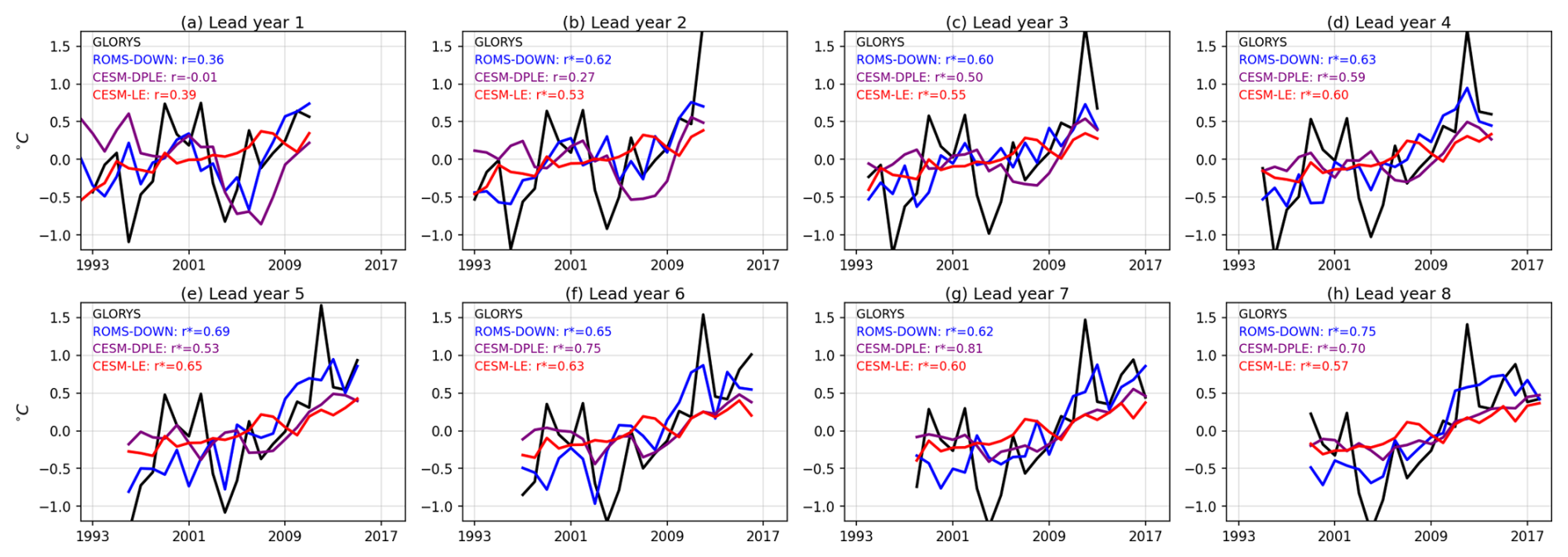
Figure 4 Time series of SST anomalies averaged over the entire NES shelf from GLORYS (black), ROMS-DOWN (blue), CESM-DPLE (purple), and CESM-LE (red) for lead years 1–8. Anomaly correlation coefficient skills (r) against GLORYS are indicated in the top left of each panel, with r^∗ indicating significance at the 95 % level based on a t-test with effective degrees of freedom accounting for autocorrelation.

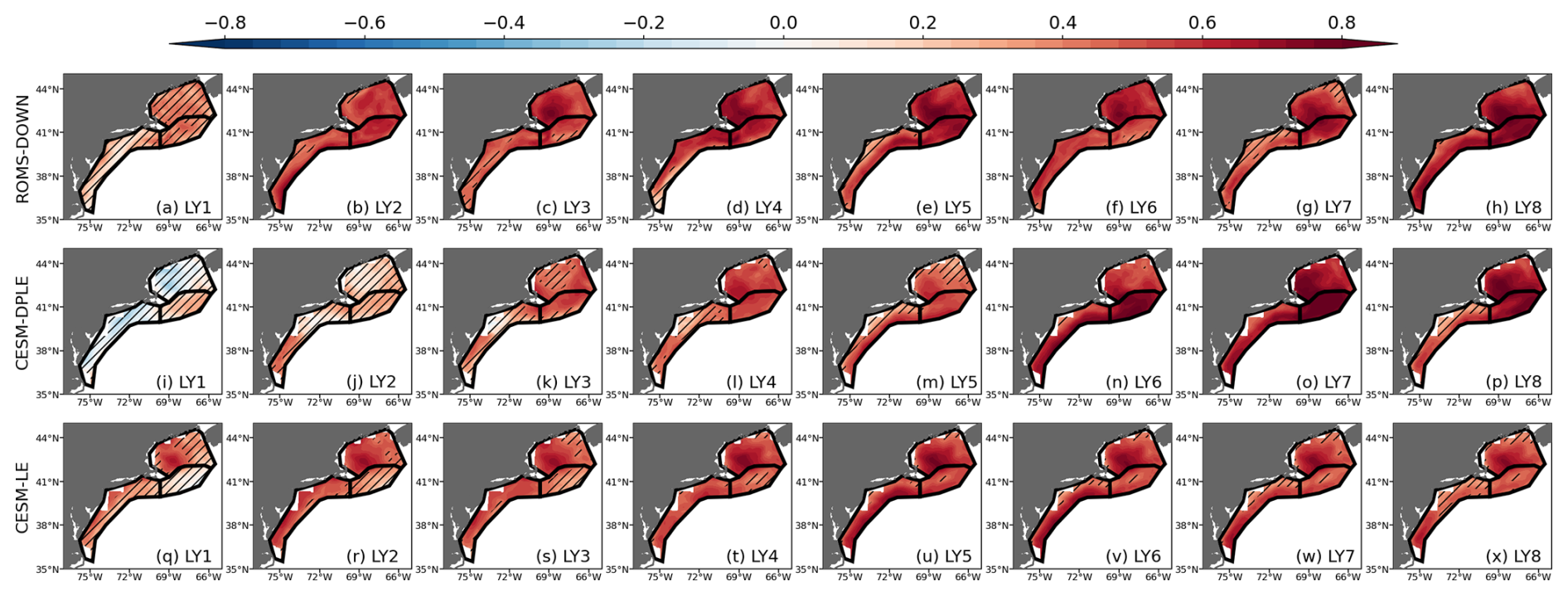
Figure 5 Anomaly correlation coefficients (ACC) for SST for lead years 1–8 (LY1–LY8) from (a–h) ROMS-DOWN, (i–p) CESM-DPLE, and (q–x) CESM-LE. ACC is computed relative to GLORYS reanalysis. Subregions outlined in black represent GOM, GB, and MAB, respectively. Hatched areas indicate regions where the ACC is not statistically significant at the 95 % confidence level.

Figure 6 ACC of the subregion-mean SST as a function of lead year (LY1–LY8) for (a) NES, (b) GOM, (c) GB, and (d) MAB. ACC values are shown for ROMS-DOWN (blue), CESM-DPLE (purple), and CESM-LE (red). Filled markers denote statistically significant correlations at the 95 % confidence level. Grey dashed line represents zero ACC skill.

Figure 5 shows the spatial distribution of ACC over the shelf, while Fig. 6 summarizes the NES-wide and subregional (GOM, GB, and MAB) mean ACC as a function of lead year, computed from spatially averaged anomaly time series. ROMS-DOWN exhibits enhanced skill generally at early lead years, with widespread positive and statistically significant correlations across the shelf in LY2–LY5. Improvements are particularly notable in the GOM and MAB, where ROMS-DOWN consistently outperforms CESM-DPLE (Fig. 6b and d). However, a consistent feature across both the regional and global prediction systems is the relatively weak ACC of SST at lead year 1 compared to longer forecast years. This reduced skill likely reflects a stronger interannual SST variability and the relatively smaller contribution of low-frequency signals during the forecast year-1 period (Fig. 4a), and may also be related to initialization error in CESM-DPLE (Yeager et al., 2018). At longer lead times (LY6–LY8), CESM-DPLE retains greater skill, which is largely attributed to the increasing influence of externally forced low-frequency variability (Fig. 4f–h). The uninitialized CESM-LE also shows surprisingly high correlations across much of the shelf. This elevated skill arises because SST variability on the NES is strongly dominated by the externally forced warming trend (Chen et al., 2020); thus, CESM-LE – of which the ensemble mean contains primarily the forced response and limited internal variability – can still reproduce much of the observed low-frequency signal. As a result, CESM-LE provides an estimate of the predictable externally forced component that both CESM-DPLE and ROMS-DOWN inherit at longer lead times.

In addition to ACC, we also evaluate forecast performance using the ensemble-mean mean square skill score (MSSS), which measures error reduction relative to a climatological reference. The spatial distribution (Fig. A5) and regional averages (Fig. A6) of MSSS for SST show patterns broadly consistent with the ACC results, with generally positive skill across much of the NES except at the earliest lead years. ROMS-DOWN exhibits modest improvements over CESM-DPLE, particularly at shorter lead times, while skill at longer leads reflects the influence of low-frequency variability. Overall, the ACC and MSSS scores suggest that much of the SST forecast skill on the NES is linked to predictable large-scale signals and long-term trends, while ROMS-DOWN improves the prediction skill by better representing shelf-scale variability and captures higher-frequency fluctuations, particularly at shorter leads.

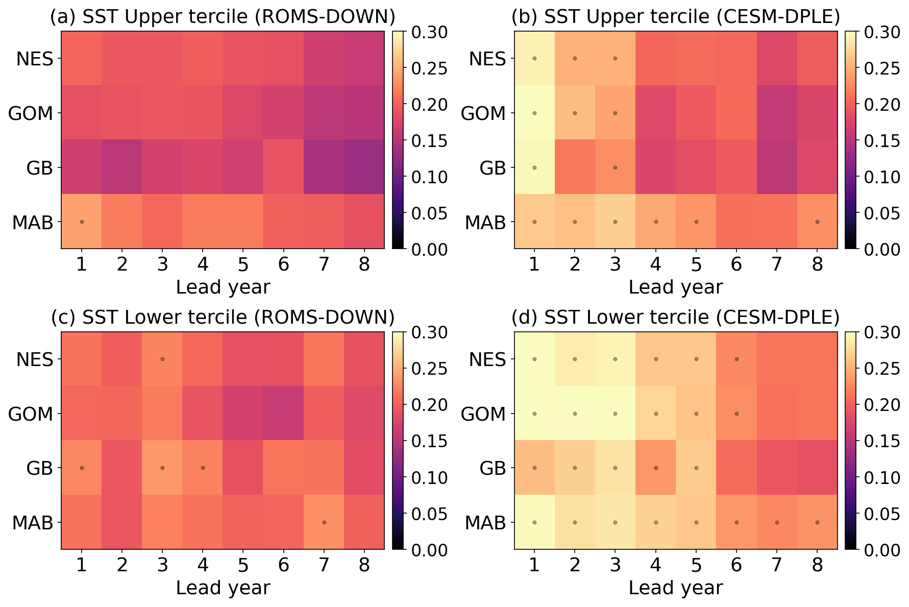
Figure 7 Brier Score for probabilistic predictions of SST tercile events on the NES. Panels (a) and (c) show the Brier Score for upper- and lower-tercile SST events, respectively, in ROMS-DOWN; (b) and (d) show the corresponding results for CESM-DPLE. Scores are calculated for the NES, GOM, GB, and MAB as a function of lead year (LY1–LY8). Lower values indicate higher prediction skill. Black dots denote values with BrS ≥ $\mathrm{2}/\mathrm{9}$, the no-skill reference value for tercile events (i.e., a climatological forecast that assigns equal probability ($\mathrm{1}/\mathrm{3}$) to each category yields an expected Brier Score of $\mathrm{2}/\mathrm{9}$, so values at or above this level indicate no improvement over climatology).

Because the long-term warming trend dominates SST variability in the NES, both ACC and MSSS show relatively high scores in the coarse-resolution CESM-DPLE, with ROMS-DOWN providing modest improvements. However, the SST time series (Fig. 4) also reveals that, even when the overall correlation or variance agreement with GLORYS is comparable, the higher resolution and improved representation of the Gulf Stream and fine-scale processes in ROMS-DOWN enable it to track warm and cool extremes more skillfully. Previous studies have shown that meridional shifts of the Gulf Stream strongly influence temperature variability over the NES, particularly in the Gulf of Maine (Pershing et al., 2015; Ross et al., 2023). Therefore, the improved representation of the Gulf Stream mean position and associated shelf–slope exchange in ROMS-DOWN likely contributes to the enhanced SST prediction skill. To evaluate this event probabilistic skill, we calculate the BrS for upper- and lower-tercile SST anomalies (Fig. 7) for CESM-DPLE and ROMS-DOWN. Consistent with the deterministic metrics, ROMS-DOWN generally produces lower (i.e., better) BrS than CESM-DPLE across most of the NES, indicating higher reliability in predicting probability of extreme events.

At longer lead times (LY6–LY8), BrS improves as externally forced low-frequency variability becomes the dominant source of skill – especially for upper-tercile warm SST events in both ROMS-DOWN and CESM-DPLE – but ROMS-DOWN still outperforms CESM-DPLE. Recall that, in terms of ACC and MSSS, CESM-DPLE shows comparable or even higher values on these leads (Figs. 6 and A6), largely because it captures the low-frequency warming trend. The SST anomaly time series also highlights pronounced interannual variations during these long lead years (e.g., strong cooling around 2004 and warming around 2012) superimposed on the trend. Although CESM-DPLE retains high ACC and MSSS on these leads, its failure to reproduce these interannual fluctuations is revealed by poorer Brier Score performance for tercile events (Fig. 7). Furthermore, compared to warm events, CESM-DPLE produces systematically higher (i.e., poor) BrS for lower-tercile (cold) events than for upper-tercile (warm) events (Fig. 7). This asymmetry suggests that much of the apparent event-level skill in CESM-DPLE arises from its ability to capture the externally forced warming trend, which favors the prediction of warm extremes. And cold events may be more strongly influenced by regional processes such as shelf–slope exchange, episodic intrusions of subpolar waters, and wind-driven vertical mixing and entrainment associated with mixed layer deepening. Because such processes depend on realistic bathymetry, vertical resolution, and mixing parameterizations, they are better represented in the high-resolution regional model than in the coarse-resolution global system. As a result, CESM-DPLE is less able to reproduce cold extremes, leading to poorer probabilistic skill (higher BrS) for lower-tercile events.

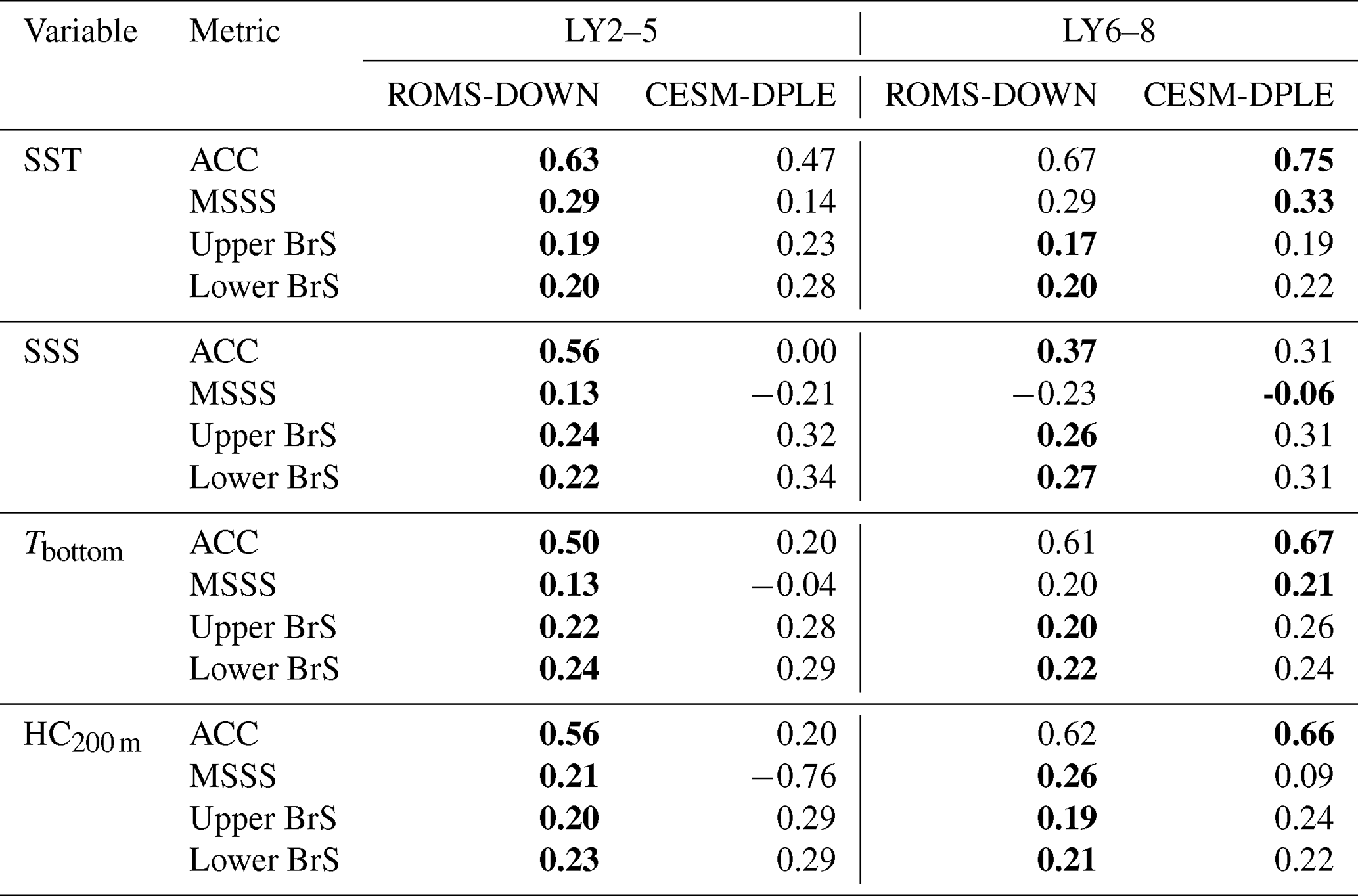
Table 1 Comparison of mean prediction skill between ROMS-DOWN and CESM-DPLE over the NES. Skill metrics are averaged over lead years (LY) 2–5 and 6–8 to summarize the early- and late-lead forecast performance, respectively. For ACC and MSSS, larger values indicate higher deterministic skill, whereas for BrS, smaller values indicate higher probabilistic skill. Bold values indicate the model with the higher skill (higher ACC and MSSS, lower BrS) for each lead-year range.

3.3 Predictability of NES Water Properties

Building on the SST prediction skill assessment, we next examine whether dynamical downscaling improves prediction skill for other key NES water properties, including SSH, SSS, T_bottom, and HC_200 m. Figure 8 shows the differences in ACC, MSSS, and BrS between ROMS-DOWN and CESM-DPLE for these variables, summarized across the entire shelf and its subregions as a function of lead year. To facilitate comparison among variables and skill metrics, Table 1 summarizes the mean prediction skill over the NES during the early (LY2–5) and late (LY6–8) forecast periods. Unlike the other variables, SSH exhibits generally weak prediction skill in both ROMS-DOWN and CESM-DPLE throughout the forecast period (Fig. A8). Although ROMS-DOWN substantially improves the mean-state representation and temporal variability of SSH relative to CESM-DPLE (Figs. 2 and 3), these improvements do not translate into enhanced SSH prediction skill. This limited improvement likely reflects the difficulty of accurately predicting offshore Gulf Stream path variability and associated mesoscale activities, which strongly influence SSH variability over the shelf (Gawarkiewicz et al., 2012; Guo et al., 2023).

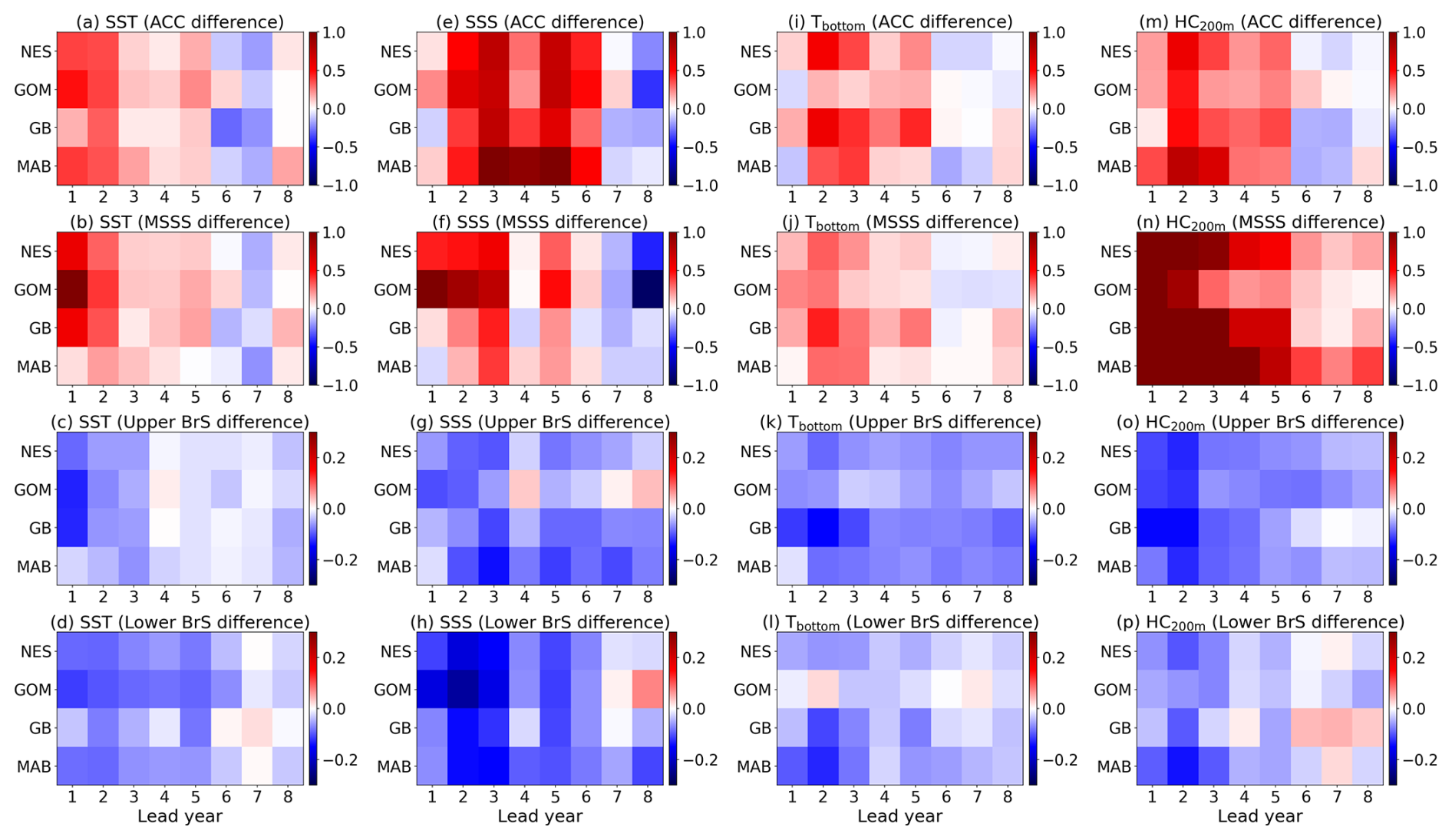
Figure 8 Differences in prediction skill between ROMS-DOWN and CESM-DPLE across the NES for multiple water properties. Panels (a)–(d) show ACC differences for SST, SSS, T_bottom, and HC_200 m; (e)–(h) show MSSS differences. Positive values (red) indicate higher skill in ROMS-DOWN, while negative values (blue) indicate higher skill in CESM-DPLE. Panels (i)–(l) show Brier Score (BrS) differences for upper-tercile events, and (m)–(p) show BrS differences for lower-tercile events. Negative values (blue) indicate lower BrS and thus greater probabilistic skill in ROMS-DOWN relative to CESM-DPLE, while positive values (red) denote better performance in CESM-DPLE. Values are averaged across the full shelf (NES) and subregions (GOM, GB, MAB) as a function of lead year (LY1–LY8).

For SST, the skill differences (Fig. 8a and e) further confirm that ROMS-DOWN's improvements are most pronounced during the first five lead years, reflecting our regional model's ability to better resolve shelf dynamics, Gulf Stream position, and mesoscale variability. Similar enhancements are evident for SSS in lead years 1–6 to a generally greater extent than SST (Fig. 8b and f), consistent with the pronounced interannual variability in SSS (e.g., Fig. 10), which is better represented in ROMS-DOWN. The BrS difference indicates that ROMS-DOWN provides higher reliability in predicting cold and freshening events in SST and SSS (Fig. 8m and n), whereas CESM-DPLE consistently shows weaker skill for lower-tercile anomalies that are influenced by unresolved regional processes mentioned above in Sect. 3.2. For subsurface properties, ROMS-DOWN again improves skill relative to CESM-DPLE. For T_bottom, improvements are most evident in the lead years 1–5, when bottom-layer variability is strongly influenced by shelf bathymetry and stratification, processes that are not well represented in CESM-DPLE. For HC_200 m, the advantage is most pronounced in MSSS, with widespread positive differences persisting across all lead years. The better agreement of the high-resolution regional model with GLORYS may be related to its finer vertical resolution, more realistic shelf bathymetry, and improved representation of vertical mixing and entrainment processes which together likely contribute to a more accurate simulation of the vertical structure and timing of variability.

The magnitude and persistence of these skill differences also vary across subregions (Fig. 8), particularly for variables and lead times where regional processes are expected to play a larger role. In the Gulf of Maine, skill improvements are generally more modest – especially for subsurface variables – likely reflecting the strong influence of upstream slope-water variability that is partly captured by CESM-DPLE. In contrast, the Middle Atlantic Bight tends to exhibit larger improvements in ROMS-DOWN for salinity and subsurface variables, especially at early lead times. This likely reflects the poorer performance of CESM-DPLE in this region, where Gulf Stream overshooting (Fig. 2) and the narrow shelf bathymetry (Fig. 1) are not well represented. Skill over Georges Bank is more variable and generally weaker, possibly due to strong tidal mixing and locally driven circulation variability that limit deterministic predictability and reduce the contribution of low-frequency, predictable signals.

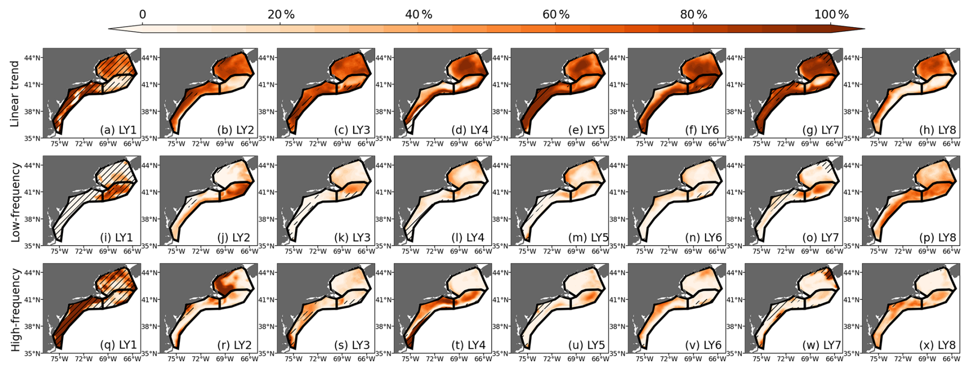
Figure 9 Decomposition of ACC(SST) in ROMS-DOWN. The total ACC is partitioned into the relative contributions (%) from (a–h) the linear trend, (i–p) low-frequency variability (periods > 10 years), and (q–x) high-frequency variability (periods < 10 years). Contributions are calculated as percentage of the squared ACC associated with each component. Hatched areas mask regions where the total ACC is not statistically significant at the 95 % confidence level.

Across metrics, the complementarity of ACC, MSSS, and BrS provides important insights into the sources of predictability. ACC reveals where models capture (or fail to capture) the phasing of anomalies. MSSS shows reductions in mean bias and error amplitude, while BrS directly evaluates the reliability of probability for discrete events. Together, these metrics suggest that while CESM-DPLE has skill at longer leads (LY6-LY8) through its representation of externally forced low-frequency variability, ROMS-DOWN tends to improve prediction skill at shorter leads and in shelf regions where regional dynamics matter most. As summarized in Table 1, ROMS-DOWN generally provides higher deterministic (ACC and MSSS) and probabilistic (BrS) skill during LY2–5, whereas the differences become smaller for several metrics during LY6–8. The improved representation of shelf–slope exchange, freshwater pathways, and vertical stratification in ROMS-DOWN may contribute to reduced mean-state biases, enhanced skill in bottom and upper-ocean heat content, and improved reliability for extreme events. While CESM-DPLE retains an advantage during periods when externally forced signals dominate – such as the shelf-wide warming observed over the analysis period (Fig. 4) – ROMS-DOWN appears to provide greater regional skill by better representing interannual-to-decadal variability.

3.4 Contributions from different timescales

To further investigate the sources of improved prediction skill in ROMS-DOWN, we decompose the anomaly correlation coefficient (ACC) into contributions from the linear trend, low-frequency variability (periods > 10 years), and higher-frequency variability. This decomposition is performed by sequentially removing components from both the predicted and observed anomaly time series (Fig. A7) and recomputing ACC at each step. Specifically, ACC is first calculated using the full anomaly time series. To quantify the relative contributions to total forecast skill, we use the squared ACC as a measure of explained anomaly variance. The contribution from the linear trend is estimated from the reduction in squared ACC after removing a linear trend from both the predicted and observed series. The detrended series is then high-pass filtered using a Butterworth filter with a 10-year cutoff period, applied independently to the predicted and observed lead-year time series using reflection padding to reduce edge effects. The squared ACC of the filtered series represents the contribution from variability on timescales shorter than 10 years. The remaining contribution, attributed to decadal and longer-timescale variability, is defined as the residual difference between the squared ACC of the detrended series and that of the high-pass filtered series. This decomposition provides a quantitative assessment of the relative roles of externally forced trends versus internal climate variability in shaping the overall skill.

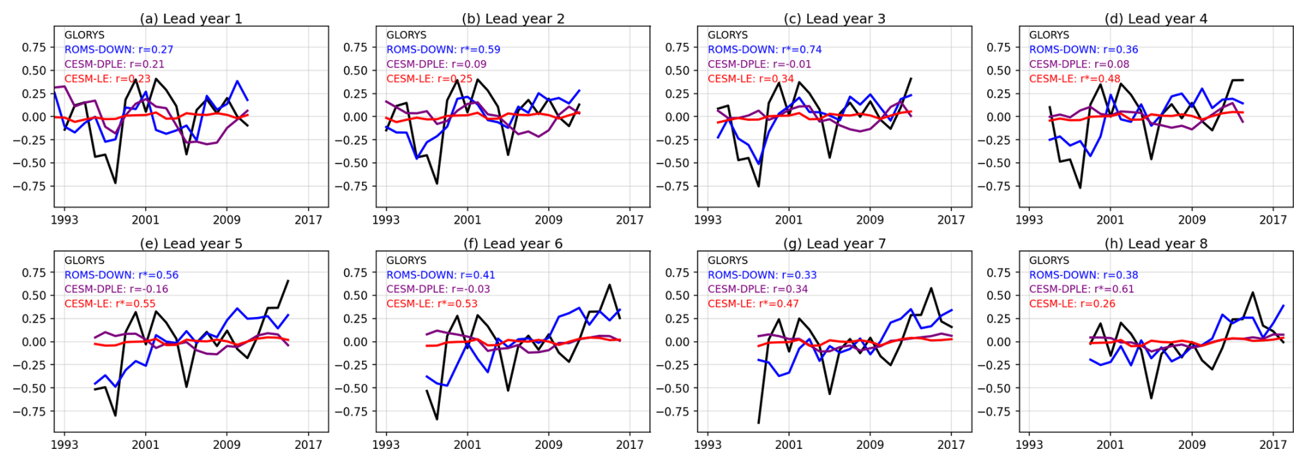
Figure 10 Time series of SSS anomalies averaged over the entire NES shelf from GLORYS (black), ROMS-DOWN (blue), CESM-DPLE (purple), and CESM-LE (red) for lead years 1–8. Correlation coefficients (r) and significance levels (p-values) between each model and GLORYS are indicated in the top left of each panel, with r^∗ indicating significance at the 95 % level.

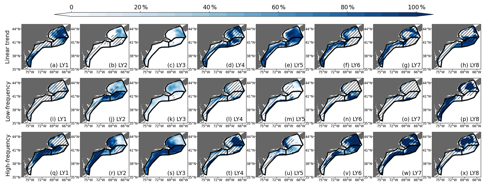
Figure 11 Decomposition of ACC(SSS) in ROMS-DOWN. The total ACC is partitioned into the relative contributions (%) from (a–h) the linear trend, (i–p) low-frequency variability (periods > 10 years), and (q–x) high-frequency variability (periods < 10 years). Contributions are calculated as percentage of the squared ACC associated with each component. Hatched areas mask regions where the total ACC is not statistically significant at the 95 % confidence level.

Taking SST as an example, the decomposition of the time series (Fig. A7) and the corresponding ACC contributions (Fig. 9) show that a large fraction of the prediction skill in ROMS-DOWN is attributable to the linear trend, particularly at longer lead times (LY6–LY7). This suggests that much of the correlation skill derives from the externally forced warming signal, consistent with the finding that CESM-DPLE and CESM-LE also perform well when evaluated at longer leads. However, the linear trend over this short period may also reflect low-frequency internal variability rather than purely external forcing, which may partly explain the reduction of trend-related ACC at LY8 in the GB and MAB regions (Fig. 9h). At shorter lead times (LY1–LY5), however, interannual-to-decadal variability contribute more to SST forecast skill, suggesting that the regional downscaling adds value by better resolving internal variability driven by regional processes that are not well represented in the coarse-resolution global model. Even though the contribution from high-frequency variability is generally small compared to the trend component, it plays a non-negligible role in certain subregions. In the MAB and GB, for example, where shelf–slope exchange, Gulf Stream and mesoscale activity strongly influence shelf water conditions, high-frequency contributions exceed 20 % of the total ACC in the early lead years (Fig. 9q–t). This highlights the capacity of the high-resolution model to represent fine-scale dynamics that are not resolved in the coarse global system. Overall, this decomposition emphasizes that while much of the skill in SST predictions arises from predictable large-scale and trend-driven signals, the improvement of ROMS-DOWN lies in its ability to capture interannual-to-decadal variability and some higher-frequency processes that influence the shelf. It also suggests that high ACC or MSSS values do not necessarily imply that the models are skillfully capturing regional variability at all timescales, but may instead reflect dominance of low-frequency trend signals. The added value of regional downscaling may become more pronounced on shorter timescales, such as seasonal predictions, where regional dynamics and improved initialization could play a larger role.

Unlike SST, whose forecast skill primarily arises from externally forced low-frequency variability, the sources of SSS forecast skill reflect complex contributions among trend, low-frequency, and high-frequency variability. Because SSS in the NES is strongly influenced by smaller-scale shelf dynamics and regional freshwater input (Gawarkiewicz et al., 2022; Ryan et al., 2024), salinity anomalies exhibit pronounced interannual-to-decadal variations on the shelf, with relatively smaller contributions from the long-term trend or low-frequency variability, particularly during lead years 1–4 (Figs. 10 and 11). Both CESM-DPLE and the uninitialized CESM-LE exhibit weak SSS variability and do not reproduce the observed shelf-wide freshening and salinification events (Fig. 10). In particular, CESM-LE exhibits very weak SSS variability. For example, the freshening event captured in GLORYS in 1998 (Wallace et al., 2018) – associated with advection of freshwater along the Slope Sea (not shown) – was skillfully represented only in ROMS-DOWN in all lead times including 1998, i.e., LY1-LY6. These events are absent in CESM-DPLE and CESM-LE, suggesting that although the large-scale interannual variability is present in the global model, its expression on the shelf is not well represented. The improved performance in ROMS-DOWN likely reflects its more realistic representation of shelf bathymetry and coastal processes, which allow large-scale salinity anomalies to be more effectively translated onto the shelf. Variability in Gulf Stream position and meandering modulates salinity in the Slope Sea, which subsequently influences shelf salinity through water mass exchange. Although freshwater inflow from rivers and estuaries contributes to the mean salinity structure through the prescribed climatological river forcing, the absence of interannual river variability in our experimental design indicates that the enhanced SSS skill in ROMS-DOWN primarily arises from its ability to dynamically translate basin-scale salinity anomalies onto the shelf. This mechanism is further discussed using the 1998 freshening event in Sect. 3.6. The enhanced ACC skill of SSS in ROMS-DOWN is particularly evident in the MAB (Fig. 8b), where the interplay between coastal freshwater plumes and slope water intrusions drives relatively strong interannual variations in salinity (Ryan et al., 2024), consistent with the notable contribution from high-frequency variability to the overall ACC skill in the MAB (Fig. 11q–x). Although a larger contribution from higher-frequency variability does not necessarily imply higher overall ACC, it indicates that the model effectively represents a broader spectrum of salinity variability, including processes that the coarse-resolution global model fails to capture. The larger skill improvement in this region likely also reflects limitations in CESM-DPLE's representation of shelf bathymetry and offshore Gulf Stream structure, which reduce the fidelity of shelf salinity variability, whereas the higher-resolution regional configuration provides a more realistic representation of these processes.

3.5 Prediction of two key shelf processes

Skillful multi-year prediction of physical conditions on the NES has the potential to support ecosystem-based management by providing advance information on environmental variability that influences marine habitats, productivity, and fisheries resources. Here we discuss the prediction of two key physical phenomena on the NES, MAB cold pool and the GOM slope-water mixture, because they translate basin-scale signals into shelf conditions that have direct ecological and management importance. The cold pool regulates summer bottom temperatures and stratification across major demersal fishing grounds, while the relative fractions of different slope-water sources entering the GOM through the Northeast Channel control deep hydrography and nutrient supply (Link et al., 2002; Townsend et al., 2010; Miles et al., 2021). Both features are tracked as ecosystem indicators in regional assessments and are central to understanding habitat for commercially important species (Pershing et al., 2015). Evaluating prediction skill for these two process-based indicators therefore tests whether regional downscaling not only improves large-scale skill metrics but also provides information that is decision-relevant for fisheries and ecosystem management.

3.5.1 Prediction of the MAB cold pool

Although CESM-DPLE provides relatively skillful large-scale predictions of SST and upper-ocean heat content in particular in longer lead years, it does not resolve important processes on the NES. One notable example is the MAB cold pool, a distinct subsurface thermal feature that integrates interactions among stratification, air-sea heat flux, advective heat fluxes, and cross-shelf exchange (Bigelow, 1933; Fratantoni and Pickart, 2007; Lentz, 2017; Chen and Curchitser, 2020) which is not well represented in CESM-DPLE. The coarse horizontal and vertical resolution of the global model with Gulf Stream overshooting prevents it from capturing the sharp vertical stratification and cross-shelf temperature gradients required for cold pool formation, resulting in a weak and diffuse temperature field that does not clearly represent the observed cold pool structure (Fig. 2r). Given that ROMS-DOWN demonstrates better performance and improved forecast skill for key water properties on the MAB shelf, it is important to evaluate whether these improvements translate into a more realistic simulation of the MAB cold pool, a feature fundamental to the physical and ecological dynamics on NES (Fratantoni and Pickart, 2007; Miles et al., 2021).

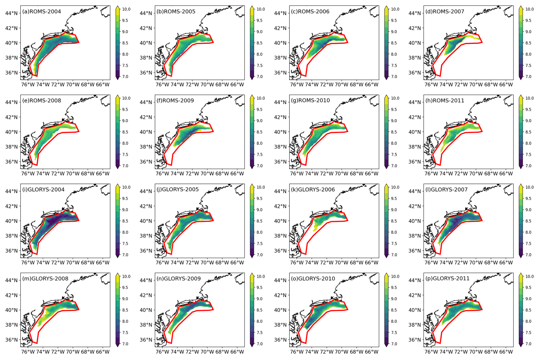
Figure 12 Annual mean vertically averaged temperature within the identified MAB cold pool layer from (a–h) the ROMS-DOWN averaged across the ensemble members and lead years and (i–p) GLORYS for 2004–2011.

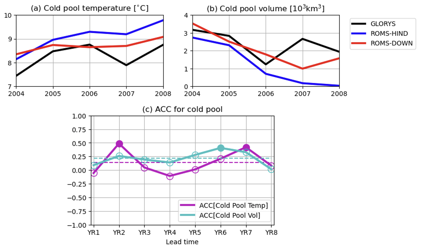
Figure 13 (a) Annual mean cold pool temperature and (b) cold pool volume from GLORYS (black), ROMS-HIND (blue), and ROMS-DOWN (red) averaged across the ensemble members and lead years during 2004–2011. (c) ACC of cold pool temperature and cold pool volume in ROMS-DOWN as a function of lead year (LY1–LY8). The dashed line indicates the mean ACC over all the lead years. Only filled markers are statistically significant at the 95 % confidence level.

The cold pool forms each spring and summer when surface heating and stratification isolate the dense, cold winter bottom water from the warmer surface layer. It typically occupies the northern shelf region in MAB and persists through early fall until mixing erodes the vertical temperature gradient. Following Chen and Curchitser (2020), the cold pool can be identified in GLORYS and ROMS-DOWN using three criteria: (1) temperature below 10 °C and salinity below 34 psu, (2) a well-developed stratification, and (3) location within the MAB shelf region between the 20 and 200 m isobaths. These criteria allow for an objective comparison between GLORYS and model simulations in terms of cold pool structure and variability. For comparison, Fig. 12 shows the annual mean, depth-averaged temperature over the identified cold pool region from GLORYS and the ensemble-mean ROMS-DOWN simulations for 2004–2008 (the cold pool is not reproduced at all in CESM-DPLE based on the above criteria). In general, ROMS-DOWN reproduces the spatial extent and structure of the cold pool with good agreement to GLORYS, capturing the tongue-shaped feature that extends southward along the shelf and the persistent cold core centered around 38–40° N. The regional model also captures more skillfully the interannual variability in cold pool intensity and volume, which is absent in the coarse-resolution global system (Fig. 13a and b). Specifically, ROMS-DOWN captures the observed warming and shrinking in cold pool in recent years (Friedland et al., 2022), consistent with GLORYS. Several key factors contribute to the improved representation of the cold pool in ROMS-DOWN, including its enhanced ability to simulate vertical thermal structure, shelf–slope exchange, and local heat advections that control cold pool formation and decay. These processes are sensitive to bathymetry and vertical resolution, which ROMS-DOWN is capable of realistically capturing.

In addition, the ACCs of cold pool temperature and volume in ROMS-DOWN show modest but positive correlations across most lead times, which indicates some degree of multi-year predictability of cold pool characteristics in the dynamical downscaling system (Fig. 13c). Although the ACC magnitude of cold pool volume is relatively low, the persistence of positive correlations through the eight lead years suggests that ROMS-DOWN captures part of the variance in cold pool evolution. However, while dynamical downscaling clearly improves the representation of the cold pool's structure and variability, it does not necessarily translate into statistically high predictability. Several factors likely limit the prediction skill even in the high-resolution regional framework. For example, the boundary and surface forcing from CESM-DPLE inherit large-scale biases and initialization errors from the global system (Yeager et al., 2018), particularly in the Gulf Stream path and subsurface heat content. In addition, air–sea heat flux variability and wind-driven mixing – both of which play a central role in winter cold pool formation and its summer erosion – contain substantial unpredictable interannual variability that limits deterministic forecast skill in the model system (Chen and Curchitser, 2020). Given the importance of vertical diffusion in driving temperature anomalies in the cold pool region (Chen and Curchitser, 2020), uncertainties in vertical mixing parameterizations in the model may further degrade multi-year predictability. Moreover, mesoscale processes such as Gulf Stream warm core rings can interact with the continental shelf (Chen et al., 2014b; Gawarkiewicz et al., 2018) and influence cold-pool evolution, which is challenging to model without data assimilation. The initialization of the cold pool is also crucial for driving its interannual variability (Chen and Curchitser, 2020). Such mesoscale and internal processes exhibit intrinsic variability that limits deterministic prediction. Therefore, while dynamical downscaling enhances physical realism, the inherent complexity and internally generated nature of the system continue to constrain its multi-year predictability.

3.5.2 Prediction of slope water mixing in GOM

A key component of NES shelf-water variability is driven by boundary inflows and the mixing of distinct slope-water masses entering through several channels, with the Northeast Channel being one of the most important pathways. The GOM is strongly influenced by the NES large-scale cyclonic circulation system. This includes the Labrador Current which brings cold, nutrient-rich water along the shelf and into the GOM through the Northeast Channel. Therefore, waters of distinct origins converge and mix within the GOM (Pringle, 2006; Townsend et al., 2010). The deep inflow through the Northeast Channel consists primarily of slope waters that are a mixture of warm, saline Warm Slope Water (WSW) originated from the Gulf Stream and cold, fresh Labrador Slope Water (LSW) advected southwestward from the subpolar North Atlantic (Mountain, 2012). These water masses, together with the overlying Scotian Shelf Water (SSW), combine to form the subsurface properties of the GOM, exerting strong control on regional temperature, salinity, stratification, and nutrient variability. The relative proportions of WSW and LSW entering the GOM vary on interannual to decadal timescales and are linked to large-scale climate forcing and Gulf Stream variability (Mountain, 2012; Seidov et al., 2021). Therefore, understanding and predicting the variability of slope-water mixing is fundamental to assessing shelf hydrographic predictability and its downstream ecological impacts.

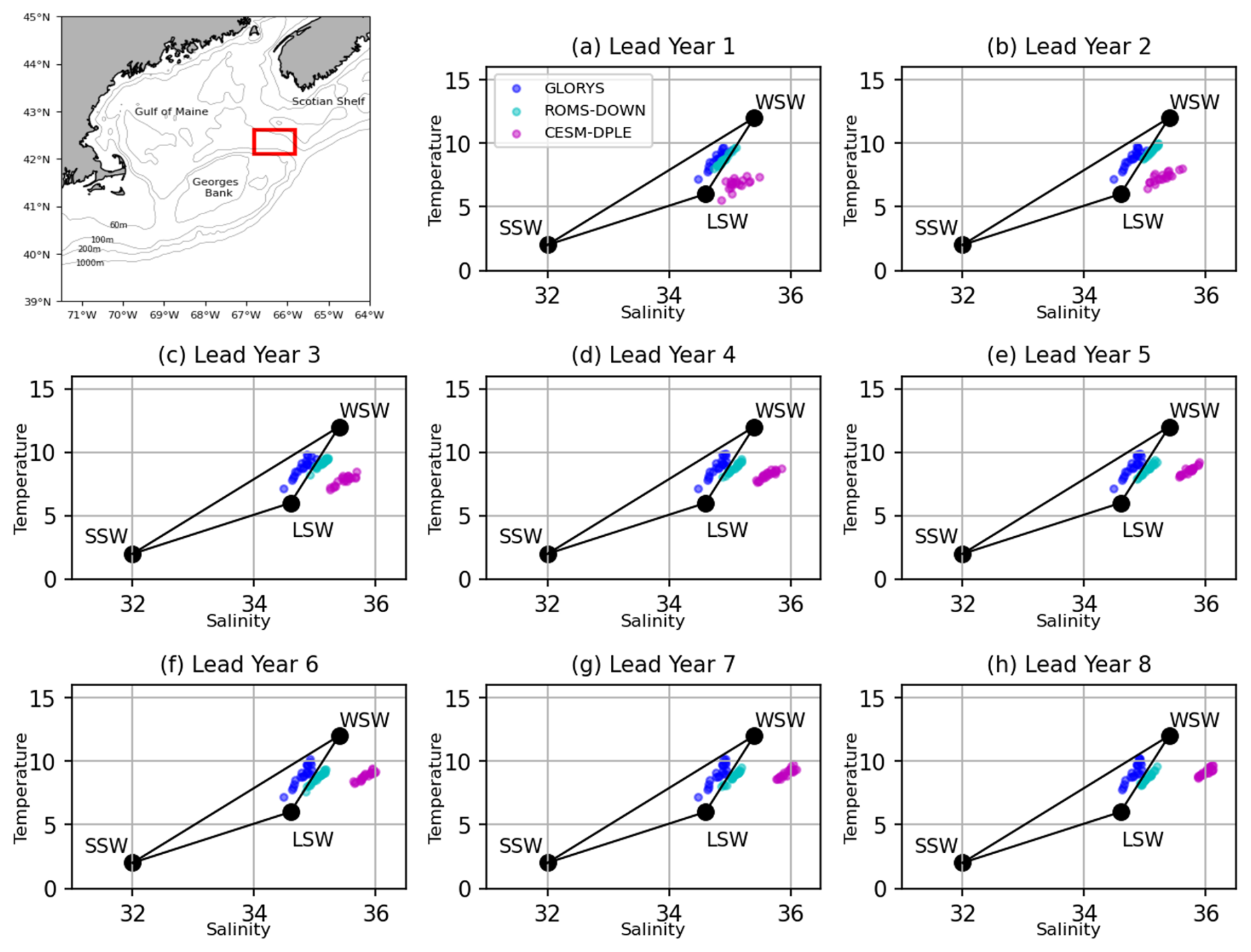
Figure 14 Temperature–salinity (T–S) diagrams showing slope water masses and their mixing in the GOM. The inset map (upper left) shows the analysis region near the Northeast Channel in the GOM (red box). Water-mass end-members include Warm Slope Water (WSW), Labrador Slope Water (LSW), and Scotian Shelf Water (SSW), following Mountain (2012). Colored dots represent depth-averaged (150–200 m) annual-mean T–S values within the analysis region from GLORYS (blue), ROMS-DOWN (cyan), and CESM-DPLE (magenta). Each dot corresponds to a different year. For ROMS-DOWN and CESM-DPLE, values are ensemble means for each year.

Following Mountain (2012), the three end-members – WSW, LSW, and SSW – form a well-defined mixing triangle. Annual-mean subsurface (150–200 m) temperature–salinity (T–S) distributions within the Northeast Channel are shown in Fig. 14 for GLORYS, ROMS-DOWN, and CESM-DPLE, covering the period 1992–2011 across all lead years of the forecast systems. GLORYS occupies a broad range primarily between the WSW and LSW end-members, consistent with substantial variability in the slope-water composition entering the GOM shown from the observational dataset in Mountain (2012). CESM-DPLE, however, exhibits an overly saline bias, likely associated with proximity of the Gulf Stream due to the overshooting. ROMS-DOWN reproduces a wider spread of T–S values, spanning much of the observed range between WSW and LSW, while its ensemble mean lies closer to the GLORYS distribution. This suggests that the regional model more skillfully represents the processes that control intermediate and deep water-mass variability in the GOM. The interannual variability of the slope-water mixture is influenced by large-scale circulation changes associated with the NAO (Mountain, 2012), as well as by oceanic intrinsic variability, including Gulf Stream meandering and eddy intrusions along the slope (Seidov et al., 2021). The improved simulation in ROMS-DOWN likely reflects its finer resolution and its ability to resolve bathymetry steering, shelf–slope exchange, and Gulf Stream variations that modulate the inflow through the Northeast Channel.

To further evaluate the model's ability to predict changes in this slope-water mixture, the forecast skill of the Labrador Slope Water fraction (% LSW) near the Northeast Channel is examined in Fig. 15. The overall positive ACC values of % LSW indicate that ROMS-DOWN retains some multi-year predictive capability for the proportion of LSW entering the GOM. The persistence of skill throughout the prediction period suggests that the model captures large-scale processes governing LSW variability, such as the southwestward transport of subpolar waters and their modulation by the NAO (Mountain, 2012). However, given the relatively short verification period, part of the increasing skill at longer leads may also reflect the influence of low-frequency variability or a trend-like signal in slope-water properties, potentially associated with broader climate-driven changes. The relatively higher skill of LSW compared to more locally influenced shelf-water properties implies that this signal is more strongly controlled by predictable basin-scale dynamics, which are preserved through initialization from CESM-DPLE and transmitted into the regional system.

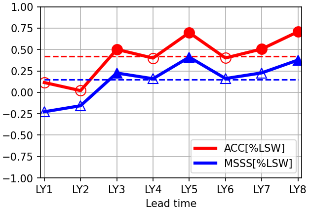
Figure 15 ACC (red) and MSSS (blue) of Labrador Slope Water fraction (% LSW) in ROMS-DOWN as a function of lead year (LY1–LY8). The dashed lines indicate the mean skill over the prediction period. Filled markers are statistically significant correlations at the 95 % confidence level.

Accurately predicting the relative contribution of % LSW also depends on the model's ability to simulate the background hydrographic structure of the shelf. Even though CESM-DPLE captures the large-scale forcing and its influence on Labrador Water transport to some extent, the representation of % LSW entering the GOM can still be biased by unrealistic local shelf conditions, such as the intrusion of warm, saline water associated with the Gulf Stream's overshooting into the region or the lack of a Northeast Channel due to coarse-resolution bathymetry. Although the MSSS values of % LSW are modest, which indicates limited amplitude accuracy, ROMS-DOWN maintains variability in slope-water composition over several forecast years. The slight offset in magnitude between ROMS-DOWN and GLORYS (e.g., saltier water masses in Fig. 14) likely reflects residual biases in the boundary conditions inherited from CESM-DPLE.

3.6 Source of multiyear predictability: a case study of the 1998 freshening event

The improved multiyear prediction skill of SSS in ROMS-DOWN suggests that regional processes play an important role in translating large-scale salinity variability onto the NES shelf. To illustrate this mechanism, we consider the pronounced freshening event observed in 1998 (Fig. 10). The spatial distribution of SSS anomalies in GLORYS (Fig. 16a) shows a strong negative anomaly extending along the shelf and slope, particularly in the MAB and GOM. ROMS-DOWN reproduces both the magnitude and spatial structure of this anomaly (Fig. 16b), whereas CESM-DPLE fails to capture this freshening event (Fig. 16c). This is consistent with the improved interannual prediction skill of SSS in ROMS-DOWN and suggests that the regional model better represents key processes associated with this event.

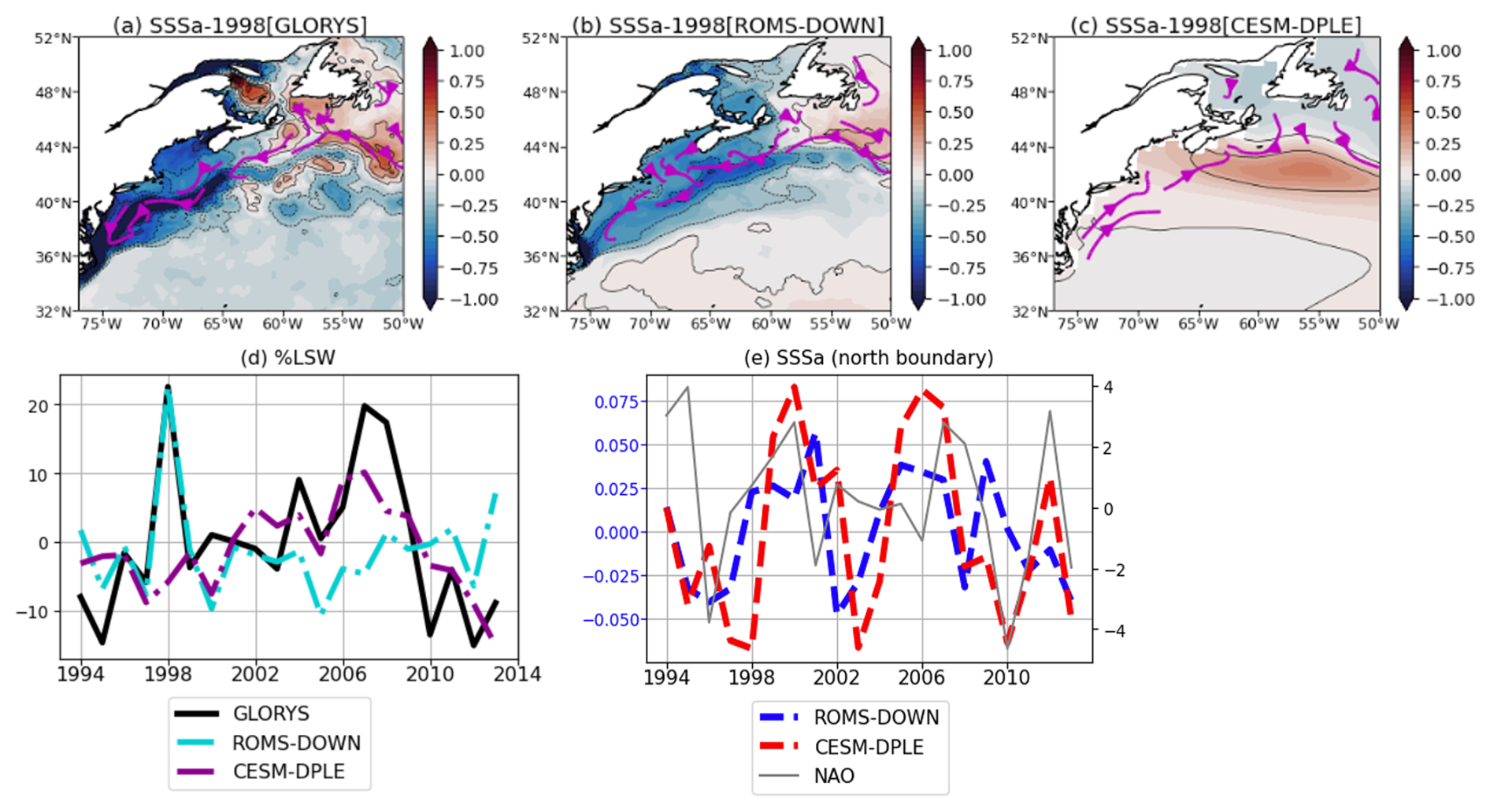
Figure 16 (a–c) Spatial maps of SSS anomalies in 1998 (a) GLORYS, (b) ROMS-DOWN, and (c) CESM-DPLE. Arrows indicate along-shelf and slope currents. (d) Time series of LSW fraction in the Northeast Channel of GOM from GLORYS, ROMS-DOWN, and CESM-DPLE. (e) Time series of SSS anomalies averaged over a narrow area near the northern boundary of ROMS-DOWN from CESM-DPLE and ROMS-DOWN, along with their relationship to the NAO. CESM-DPLE and ROMS-DOWN results are ensemble means from the 1994 start year.

Analysis of the preconditioning leading up to the event (not shown) reveals that a fresh anomaly develops in the slope waters one to two years prior to 1998 in both GLORYS and ROMS-DOWN. This indicates a large-scale origin of the signal perhaps from outside of our ROMS-DOWN domain. Consistent with this, the fraction of LSW at the entrance of the GOM (Fig. 16d) as discussed in Sect. 3.5.2 shows a pronounced increase in both GLORYS and ROMS-DOWN in 1998, which suggests enhanced southward transport of subpolar waters (currents shown in Fig. 16a and b) as a key driver of the event. However, CESM-DPLE does not capture the % LSW variation (Fig. 16d) nor the equatorward shelf and slope currents (Fig. 16c), indicating that although large-scale signals may be present, their expression on the shelf is not well represented in the coarse-resolution global system. The strong relationship between % LSW and salinity anomaly in 1998 further suggests that basin-scale forcing, potentially linked to NAO variability (Mountain, 2012), provides an important source of predictability for NES properties.

To assess whether the predictability of this event is attributable to large-scale anomalies advected from the subpolar gyre – which are prescribed as the northern boundary condition for ROMS-DOWN – we examine SSS anomalies over a narrow area near the northern boundary (Fig. 16e). ROMS-DOWN closely follows CESM-DPLE in both phase and magnitude of boundary SSS anomalies, indicating that the large-scale salinity signal is inherited from CESM-DPLE forcing by design. Despite this, CESM-DPLE fails to reproduce the corresponding shelf freshening due to lack of equatorward advection along the slope and shelf break (Fig. 16c). The large-scale salinity signal weakens as it propagates into the coastal region in CESM-DPLE, likely due to its limited representation of shelf–slope bathymetry and along-shelf transport. In contrast, ROMS-DOWN more effectively preserves and translates the inherited large-scale signal into a realistic regional response.

This case study indicates that the improved interannual prediction skill in ROMS-DOWN arises from a combination of inherited large-scale predictability and enhanced representation of regional processes, which together enable a more accurate prediction of basin-scale anomalies onto the NES.

4 Discussion

While dynamical downscaling improves the physical realism and regional predictability of NES water properties, several limitations remain that constrain overall forecast skill.

First, as shown in Fig. A8 and described in Sect. 3.3, SSH exhibits generally weak prediction skill in both ROMS-DOWN and CESM-DPLE. On the shelf, SSH variability is strongly influenced by offshore Gulf Stream fluctuations and associated mesoscale activity (Böhm et al., 2006; Ezer, 2016; Guo et al., 2023), which are inherently chaotic and difficult to predict deterministically, particularly in the absence of data assimilation, even with a dynamically downscaled regional model. In addition, uncertainties in atmospheric forcing – particularly wind stress variability – further limit predictability on multiyear time scales. The limited ability of ROMS-DOWN to fully reproduce the variability of complicated shelf circulation patterns and offshore Gulf Stream meandering may contribute to the low SSH skill and highlights the persistence of internal noise in the regional system.

A second limitation arises from the experimental design. Each ROMS-DOWN ensemble is integrated for only 8 prediction lead years and 20 start years due to limited availability of the daily atmospheric variables from CESM-DPLE to force the ROMS-DOWN as well as limited computational resources. With pronounced interannual to decadal variability, the sliding 20-year windows for different lead time prediction time series (Figs. 4 and 10) are dictated by different low-frequency temporal evolutions, e.g., 1992–2021 for LY1 vs. 1999–2018 for LY8, and thus the prediction skill differences may not be solely due to the difference in lead years. For example, the verification periods for longer lead years contain a larger contribution from the long-term warming trend than those for shorter lead years. Because this trend is relatively predictable, differences in skill among lead years may partly reflect differences in the verification periods rather than the lead time alone (e.g., Fig. 4a vs. h). This sampling difference introduces uncertainty when comparing lead-year-dependent skill across variables and regions. Extending the number of start-year simulations and lengthening each simulation would provide a more comprehensive assessment of uncertainty and improve statistical confidence in the skill estimates.

An additional source of uncertainty relates to the use of GLORYS as the verification benchmark. GLORYS does not explicitly include tidal forcing, and its representation of stratification and mixing over strongly tidal regions – such as GB and parts of the GOM – may therefore differ from ROMS simulations that include tidal harmonics. These structural differences could influence the magnitude of skill metrics, particularly for subsurface properties. However, our evaluation focuses on annual-mean anomalies with lead-time-dependent climatology removed, which reduces sensitivity to mean-state biases and high-frequency tidal variability. While the absence of tidal forcing in GLORYS is unlikely to fundamentally alter the conclusions regarding the added value of dynamical downscaling for multi-year anomaly predictability, it may contribute to differences in T_bottom and HC_200 m, particularly in strongly tidal regions such as GB and parts of GOM, through its influence on vertical mixing and heat exchange. Consequently, part of the skill differences for these variables may reflect differences in the representation of tidal mixing between GLORYS and ROMS.

Overall, while our dynamical downscaling approach enhances the representation of shelf processes and improves multi-year forecast skill, it does not yet overcome the inherent limits of predictability set by internal variability, model biases in both the global and regional models, and finite ensemble sampling. Future efforts should focus on extending hindcast periods, increasing ensemble size, ensuring that the atmospheric and oceanic output required for regional downscaling is routinely archived. In addition, improving the representation of circulation variability – for example through submesoscale-resolving configurations and the incorporation of atmosphere–ocean coupling in regional downscaled prediction systems – may yield additional gains in multi-year prediction skill on the NES.

5 Summary

This study evaluates the improvement in multi-year prediction skill achieved through dynamic downscaling on the U.S. Northeast Shelf using a high-resolution regional model forced by anomaly fields from the global prediction using CESM-DPLE system. The assessment focuses on mean-state fidelity, forecast skill metrics, and the representation of key regional phenomena, including the MAB cold pool and slope-water mixing near the Northeast Chanel. Model results are compared against the GLORYS ocean reanalysis to assess both deterministic (anomaly correlation coefficient, mean squared skill score) and probabilistic (Brier Score) performance.

ROMS-DOWN substantially reduces mean-state biases in SST, SSH, SSS, bottom temperature, and upper-ocean heat content relative to CESM-DPLE. Improvements are pronounced over the shelf and slope regions, where the higher horizontal resolution allows for a more realistic representation of cross-shelf gradients, bathymetry, and offshore Gulf Stream position. Both deterministic and probabilistic metrics demonstrate that ROMS-DOWN improves forecast skill, particularly during the first five forecast years (Table 1 and Fig. 8). At longer leads (LY6–LY8), CESM-DPLE retains comparable skill due to the dominance of low-frequency, externally forced variability. The BrS further shows that ROMS-DOWN provides greater reliability in predicting the probability of upper- and lower-tercile events than the global system, highlighting its strength in capturing event-scale variability. Decomposition of the forecast skill indicates that the sources of predictability differ among water properties. For example, much of the SST skill arises from the externally forced warming trend, which both ROMS-DOWN and CESM-DPLE capture well. Part of this trend-related skill may also reflect low-frequency internal variability projected onto the relatively short analysis period. In contrast, the ACC skill for SSS is primarily linked to interannual-to-decadal variability, where ROMS-DOWN exhibits improved multi-year prediction capability, likely because its higher-resolution bathymetry and more realistic shelf representation allow large-scale salinity variability inherited from CESM-DPLE to be more accurately transferred onto the shelf.

The MAB cold pool, a thermally stratified bottom layer that strongly influences regional temperature structure and marine ecosystems, is skillfully reproduced in ROMS-DOWN but not resolved at all in CESM-DPLE, manifested in the weaker T_bottom prediction skill in the global system (Fig. 8c, g, and k). The regional model captures the cold pool's spatial structure and its interannual variability in strength and volume, which demonstrates an improved representation of stratification and shelf–slope exchange processes. However, despite this enhanced physical realism, cold-pool predictability remains moderate, likely constrained by boundary forcing biases, parameterization uncertainties, and the intrinsic variability of mesoscale and synoptic processes. In the GOM, ROMS-DOWN also more accurately represents the mixing between shelf and slope waters entering through the Northeast Channel, reproducing the observed range of slope-water temperature and salinity variability more skillfully than CESM-DPLE. The global system exhibits a warm and saline bias, likely linked to bias in Gulf Stream separation near Cape Hatteras. The forecast skill of the LSW fraction in the Northeast Channel remains consistently positive, reflecting the influence of predictable large-scale circulation patterns – such as the westward transport of subpolar waters and their modulation by climate forcings such as the NAO. While amplitude errors remain, ROMS-DOWN captures physically meaningful multi-year variability in slope-water composition, underscoring the importance of dynamical downscaling for linking large-scale climate signals with regional hydrographic variability.

Our results complement recent work on seasonal and decadal forecasts for the NES region. Initialized decadal prediction studies show that starting from observed climate states improves regional circulation and heat-transport signals, enabling skill for North Atlantic SST and related high-latitude metrics (e.g., Yeager et al., 2015, 2018). On a seasonal scale, dynamically downscaled regional forecasts have achieved better skill on the shelf by resolving fine-scale processes along the NES (Ross et al., 2024). Extending to decadal scales, recent downscaled predictions suggest a near-term pause in shelf warming (Koul et al., 2024). Here we assess prediction skill on interannual timescales in a regional dynamical downscaling framework for the NES. While initialized climate predictions from subseasonal to decadal timescales have been widely studied (Meehl et al., 2021; O'Kane et al., 2023), the extent to which large-scale predictability can be translated into improved regional forecasts for the NES through dynamical downscaling remains less explored. Our work on multi-year prediction fills a critical gap between seasonal and decadal forecasts. In particular, the largest improvements in prediction skill occur during the 2–5 forecast years, a timescale that is especially relevant for living marine resource management because it provides outlooks beyond seasonal forecasts while remaining more actionable than decadal projections. We demonstrate that dynamical downscaling enhances the representation and multiyear prediction of NES hydrography by bridging global-scale forcing with regional processes that shape shelf variability. ROMS-DOWN improves mean-state fidelity, early-lead forecast skill, and event-level reliability. Although the predictability of features such as the shelf sea level anomaly and cold pool remains constrained by intrinsic variability and forcing uncertainties, the results highlight the potential of regional dynamical downscaling as a critical tool for advancing multi-year climate predictions and their applications to coastal and ecosystem management on the NES. Future efforts should include coordinated comparisons of regional downscaling systems in the NES (e.g., ROMS and Modular Ocean Model version 6 (MOM6) in Ross et al., 2024). Because no single model is free of bias, systematic intercomparison across models, domain configurations, and boundary forcing strategies is essential for identifying robust sources of predictability and quantifying uncertainties. Such efforts will improve confidence in downscaled climate predictions for coastal applications.

Appendix A

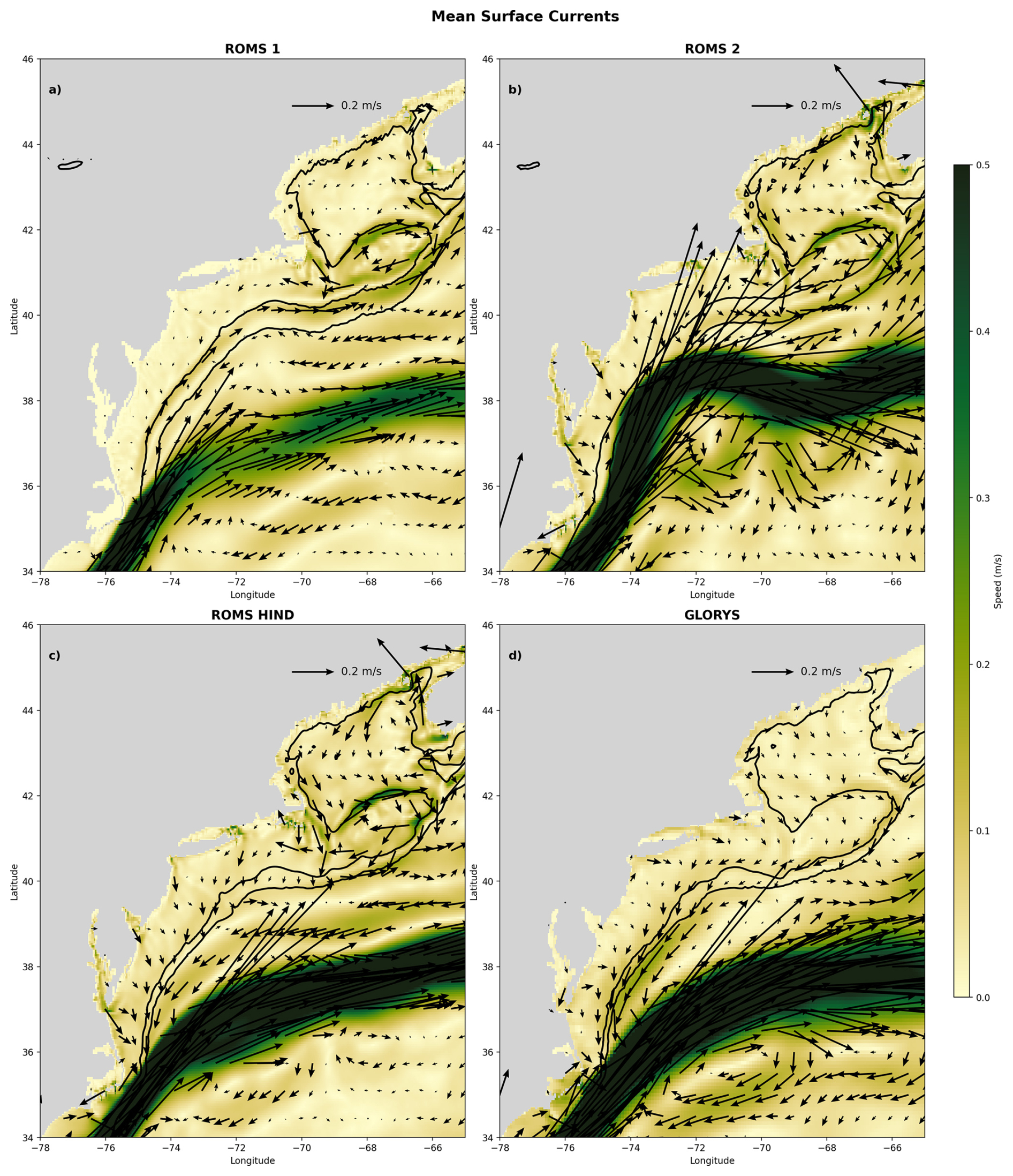
Figure A1 Five-year mean (2004–2008) surface velocity vectors and current speed (m s⁻¹) over the NES from three ROMS configurations and the GLORYS reanalysis: (a) ROMS 1 (Batteen and Miller, 2009) (smoothing, r_x0=0.1), showing a shoreward-shifted 100 m isobath around GB, a weakened equatorward shelf flow, and a weakened Gulf Stream; (b) ROMS 2 (Shapiro filter, r_x0=0.1), with an offshore-displaced 1000 m isobath near Cape Hatteras and Gulf Stream overshooting; (c) ROMS-HIND, using updated shelf bathymetry (r_x0=0.25), which is more consistent with ETOPO1, yielding improved shelf circulation and Gulf Stream pathway; and (d) GLORYS reanalysis for reference (also based on ETOPO1 bathymetry). Black contours denote the 100 and 1000 m isobaths only. Note that the shelfbreak/slope current is poleward in ROMS 1, and to a lesser extent in ROMS 2, which is likely due to the bathymetry smoothing near the Cape Hatteras, in contrast to the more realistic equatorward flow in ROMS-HIND and GLORYS.

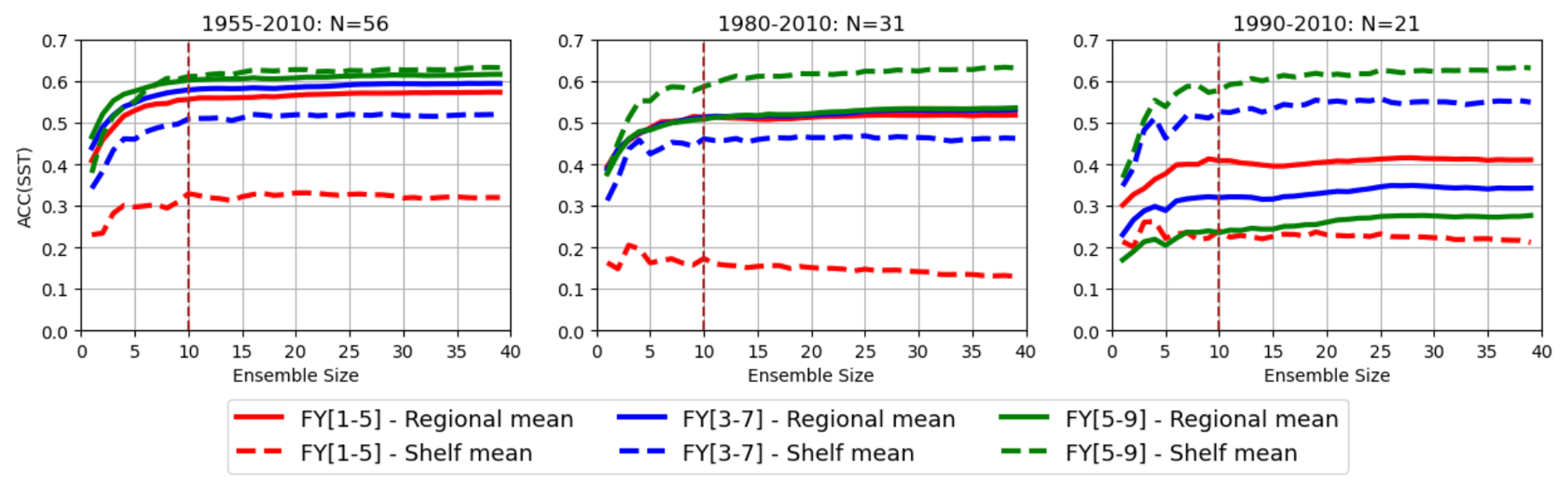
Figure A2 Sensitivity of Anomaly correlation coefficients (ACC) forecast skill in CESM-DPLE to the number of ensemble members and the number of initialization years. Each panel shows the ACCs of SST averaged over the entire domain (solid lines) and just the shelf (dashed lines) for different ensemble sizes, based on three sets of number (N) of initialization years.

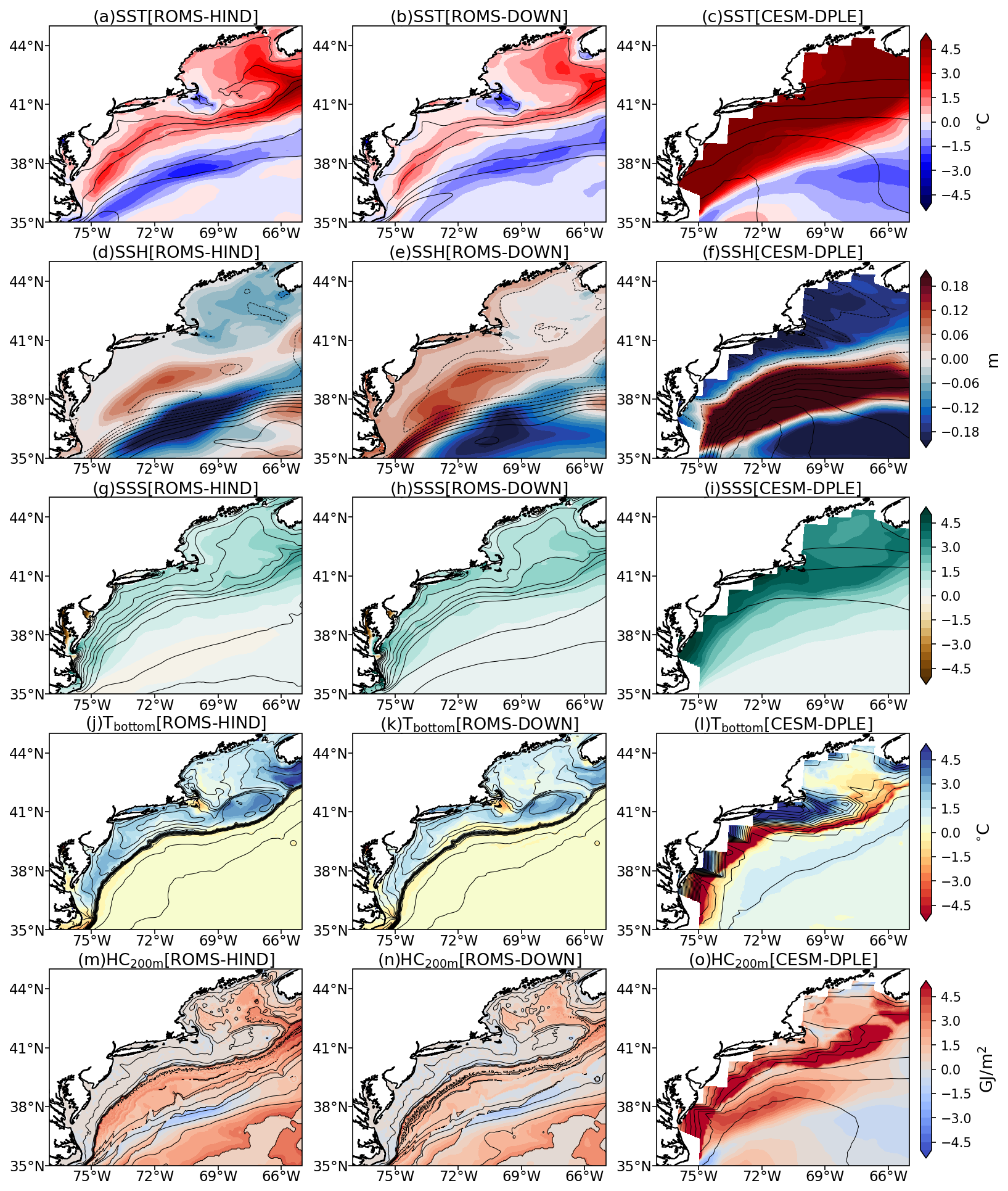
Figure A3 Spatial distribution of mean biases (model minus GLORYS) for (a–c) SST, (d–f) SSH, (g–i) SSS, (j–l) T_bottom, and (m–o) HC_200 m for ROMS-HIND (left column), ROMS-DOWN (middle column), and CESM-DPLE (right column). Biases are calculated using annual-mean fields over the period 2004–2010. Contours indicate the corresponding climatological fields.

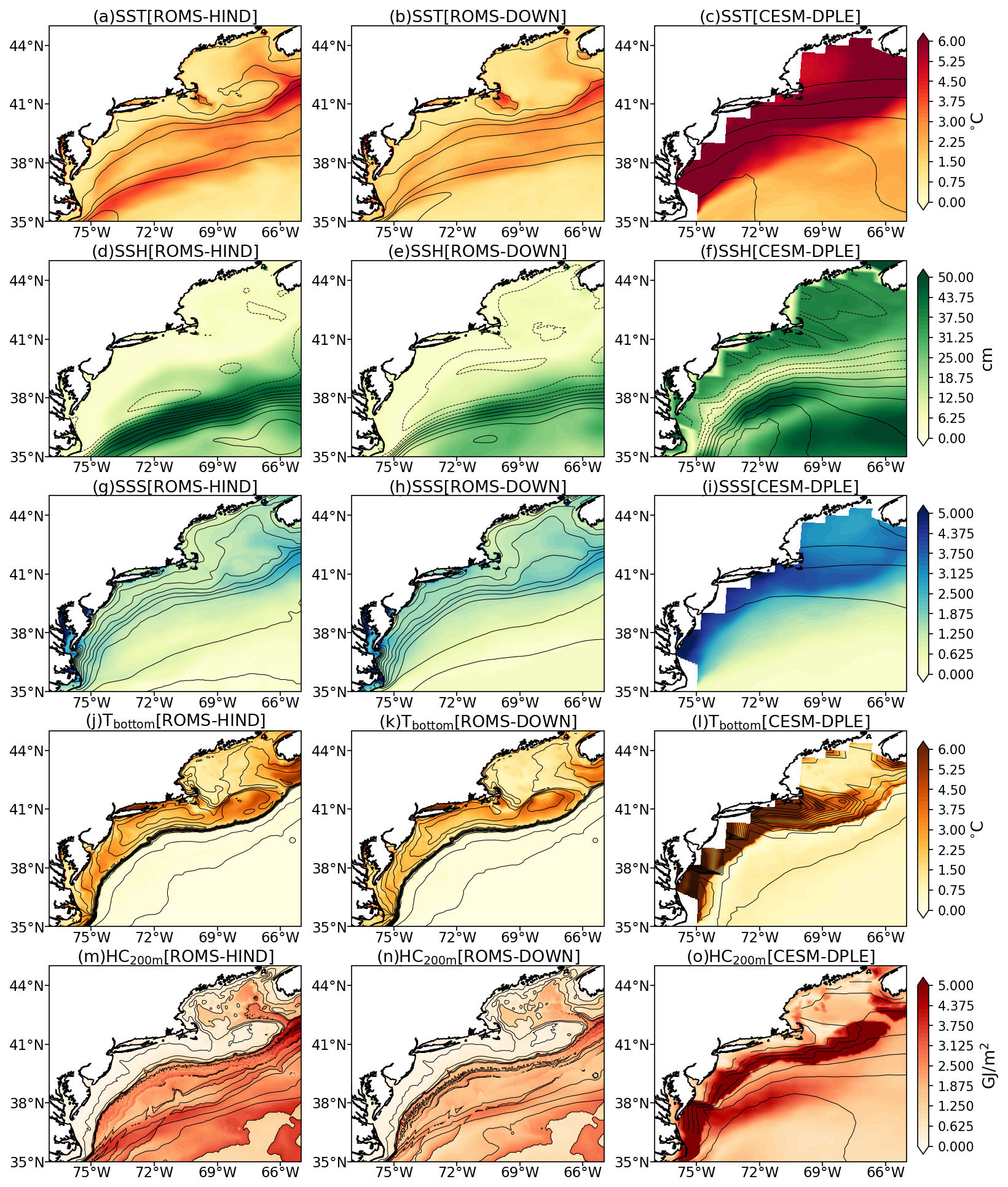
Figure A4 Spatial distribution of temporal root-mean-square error (RMSE) relative to GLORYS for (a–c) SST, (d–f) SSH, (g–i) SSS, (j–l) T_bottom, and (m–o) HC_200 m from ROMS-HIND (left column), ROMS-DOWN (middle column), and CESM-DPLE (right column). RMSE is calculated using annual-mean anomalies over the analysis period. Contours indicate the corresponding climatological fields.

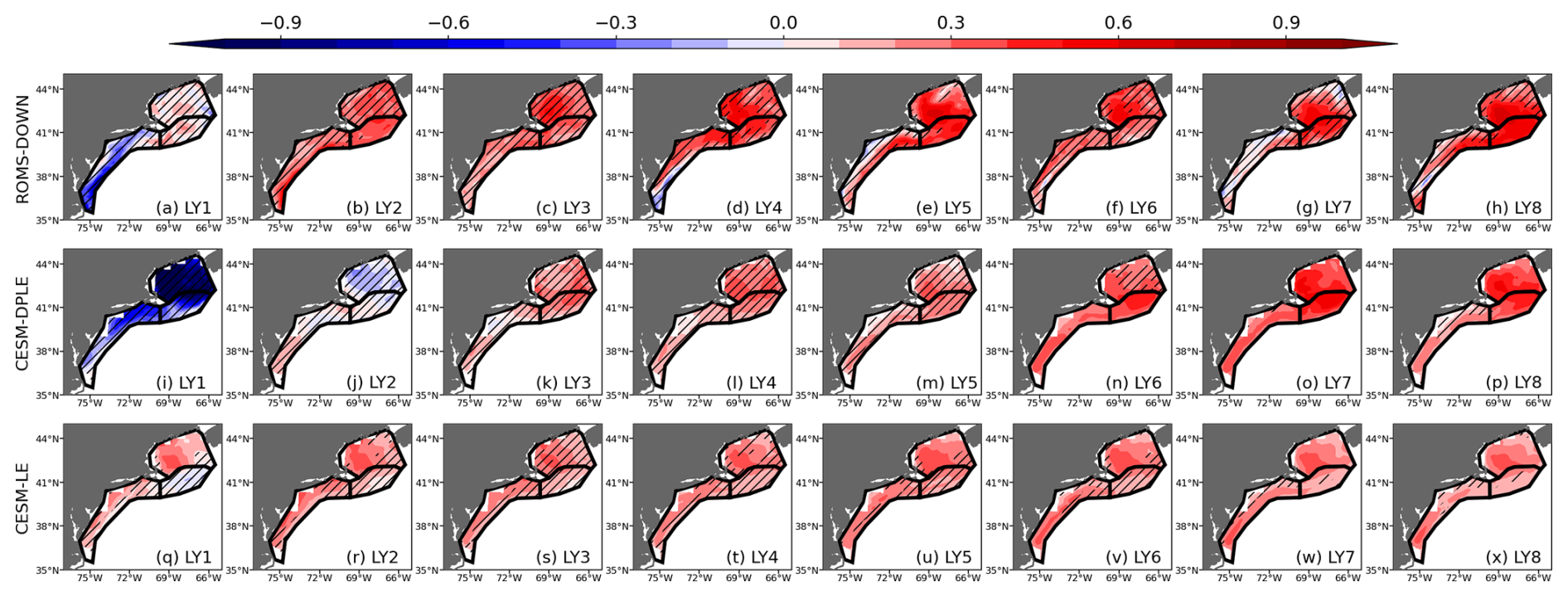
Figure A5 Mean square skill score (MSSS) of SST for lead years 1–8 (LY1–LY8) from (a–h) ROMS-DOWN, (i–p) CESM-DPLE, and (q–x) CESM-LE. MSSS is computed relative to GLORYS reanalysis. Subregions outlined in black represent GOM, GB, and MAB, respectively. Hatched areas indicate regions where the MSSS is not statistically significant at the 95 % confidence level.

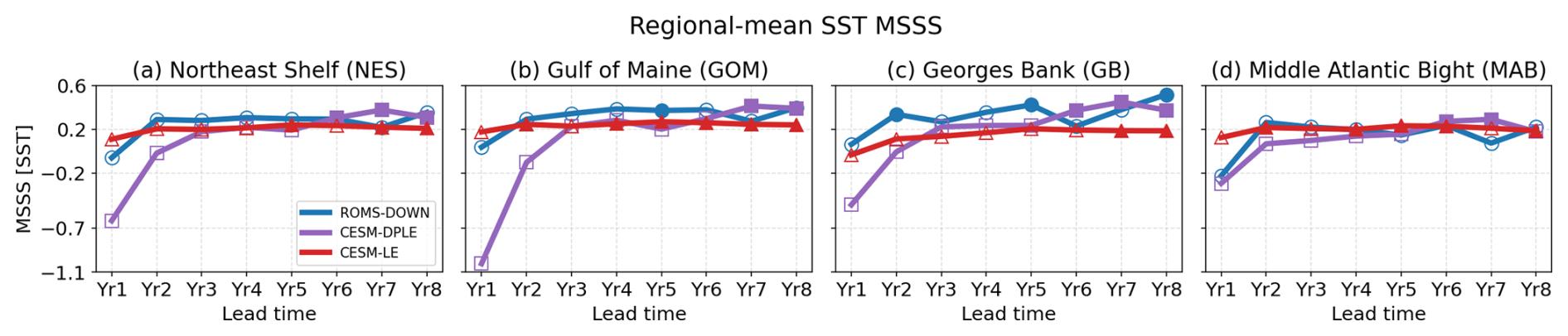
Figure A6 MSSS of the subregion-mean SST as a function of lead year (LY1–LY8) for (a) NES, (b) GOM, (c) GB, and (d) MAB. MSSS values are shown for ROMS-DOWN (blue), CESM-DPLE (purple), and CESM-LE (red). Filled markers denote statistically significant values at the 95 % confidence level. Grey dashed line denotes zero MSSS.

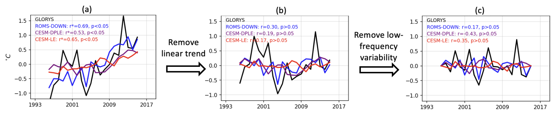
Figure A7 Similar to Fig. 4e, but showing the decomposition of the SST anomaly time series. (a) Original SST anomaly time series from GLORYS (black), ROMS-DOWN (blue), CESM-DPLE (purple), and CESM-LE (red) for lead year 5, which are identical to Fig. 4e. (b) SST anomaly time series after removing the linear trend, from which the linear-trend contribution to ACC (Fig. 11e) is derived. (c) SST anomaly time series containing only the high-frequency component (periods < 10 years) obtained using a high-pass filter, from which the high-frequency contribution to ACC (Fig. 11u) is derived. Correlation coefficients (r) and significance levels (p values) between each model and GLORYS are indicated in each panel.

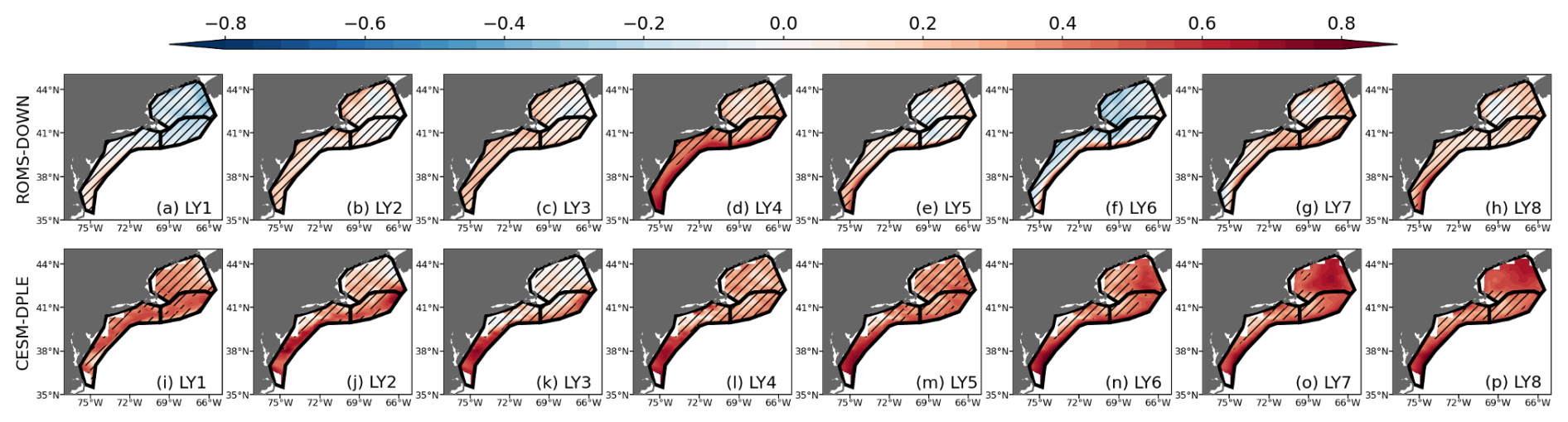
Figure A8 ACC for SSH for lead years 1–8 (LY1–LY8) from (a–h) ROMS-DOWN and (i–p) CESM-DPLE. ACC is computed relative to GLORYS reanalysis. Subregions outlined in black represent GOM, GB, and MAB, respectively. Hatched areas indicate regions where the ACC is not statistically significant at the 95 % confidence level.