A dynamical downscaling approach for the improved representation of sub-annual coastal sea level variability: the importance of shelf and slope ocean dynamics

Using a recently developed dynamical downscaling framework, we build and assess an ensemble of year-long sea level hindcasts for the western North Atlantic. Downscaled high-resolution regional ocean model (NWA12) output of US East Coast sea level at long established tide gauge stations is compared to parent coarse-resolution global ocean model (SPEAR) output to quantify varied impacts of downscaling in a forecasting framework, particularly from a daily extremes perspective. Comparisons of modeled coastal sea level distributions and observations at tide gauge stations reveal downscaling enhances variability by a factor of two to ten across all resolved frequencies. As the downscaled simulations are forced at the surface with the same atmosphere felt by the SPEAR ocean, we attribute this enhanced variability to the improved representation of shelf and slope ocean dynamics. The magnitude of this enhancement, however, appears a strong function of latitude and suggests that the added value of downscaling varies geographically. Together, these results demonstrate how dynamical downscaling can offer application-relevant time varying statistics of higher frequency coastal sea level variability, like planning based on inundation return periods, and an improved understanding of the links between model resolution and the processes driving coastal sea level changes.

1 Introduction

Coastal sea level variability across hourly to monthly timescales comprises predictable contributions from the tides and seasonal cycle, but also contributions from a less predictable combination of atmospheric and ocean dynamics (e.g., wind-driven transport, boundary current variability, coastally trapped waves, inverted barometer effects). Potential predictability of these contributions can be distilled from a dynamical understanding of circulation along ocean margins, long observational records at coastal tide gauge stations, and simulations of varied complexity of continental shelf dynamics. Different approaches have sought predictive skill through the use of: simplified barotropic models and data assimilation (Rose et al., 2024), statistical approaches (Long et al., 2023), and damped persistence frameworks (Dusek et al., 2022) that reduce system complexity or isolate specific processes. These efforts all reflect a desire and need to characterize, understand, and predict coastal variability, especially extreme event occurrences associated with flooding (Thompson et al., 2021). What is often absent in these approaches, however, as a result reductions in system or model complexity, is full consideration or representation of three dimensional continental shelf and slope ocean dynamics that shape connectivity between the coast and larger-scale or remote ocean and atmosphere dynamics. Resolving this coast-to-open-ocean transition is necessary to gain a process-level understanding of the drivers of coastal sea level change which can bolster interpretation of forecast skill.

At a process level, coastal sea level variability can be considered from local and remote perspectives. Locally, atmospheric pressure and wind forcings primarily drive variability moderated by shelf circulation and boundary currents (Lentz, 2024; Camargo et al., 2025). This variability is then influenced by remote forcings communicated through either the coastal wave guide (Hughes and Williams, 2010; Wise et al., 2020) or Rossby waves impinging along a western boundary (Calafat et al., 2018). Ocean model representation of both local and remote drivers of higher frequency coastal variability is fundamentally linked to horizontal model resolution of the ocean, atmosphere, and bathymetry (Li et al., 2022; Little et al., 2026). The importance of bathymetric resolution, however, is not universal and depends on continental shelf width and local deformation radii. Where the shelf is narrow, enhanced connectivity between the coast and open ocean implies that more realistic simulations and accurate forecasts may be achieved to the extent that larger-scale dynamics and coastal waves are well resolved (Jacox et al., 2023; Little et al., 2024; Alexander et al., 2025). Where the shelf is relatively wide, realistic simulations of coastal sea level depend on the resolution-dependent representation of near-coast dynamics and smaller-scale processes.

Along the US East and Gulf coasts, continental shelf width varies greatly, from ∼ 10 to ∼ 200 km, thus variably linking the coast and open ocean. Much previous work has explored relationships among US East Coast sea level and flooding events (Volkov et al., 2023), winds (Wang et al., 2022), coastal waves (Wise et al., 2020), bathymetry (Wise et al., 2018), the Gulf Stream (Donatelli et al., 2025; Wu and He, 2025), and the Atlantic Meridional Overturning Circulation (AMOC) (Ezer and Atkinson, 2014; Little et al., 2019). While spatial patterns of coastal variability strongly depend on timescale, distinct regimes are found to the north and south of Cape Hatteras, North Carolina. This region corresponds geographically to a significant narrowing of continental shelf width and is the location where the Gulf Stream separates from the coast and turns eastward. Partly as a result of this geography, sea level and along-shore winds are more tightly linked north of Cape Hatteras (Wang et al., 2022), while Gulf Stream strength and positioning modulate coastal sea level south of Cape Hatteras, also influenced by equator-ward propagating coastal waves (Wang et al., 2024). These two regimes can be understood to reflect differing contributions of offshore, wind-driven, and coastal wave dynamics (Wise et al., 2018), but also continental shelf width (Minobe et al., 2017). From a modeling perspective, accurate simulation of ocean behavior in this region is centrally linked to the representation of the shelf and slope transition.

In the construction and configuration of ocean models used to explore and forecast coastal sea level variability, tradeoffs must be made between computational cost, domain size, horizontal and vertical resolution, and process representation that together leverage knowledge of coastal margin hypsometry. Dynamical downscaling enables a more realistic representation of coastal sea level variability, influenced by both local and remote processes and across the coastal to open-ocean transition. Relatively coarse horizontal resolution parent global climate model output can be used as boundary forcings driving a higher horizontal resolution ocean model. This results in enhanced resolution of local shelf/slope dynamics that feel larger scale and remote weather and climate forcings (Ross et al., 2024; Liu et al., 2016; Hermans et al., 2020; Apecechea et al., 2025; Suzuki et al., 2026).

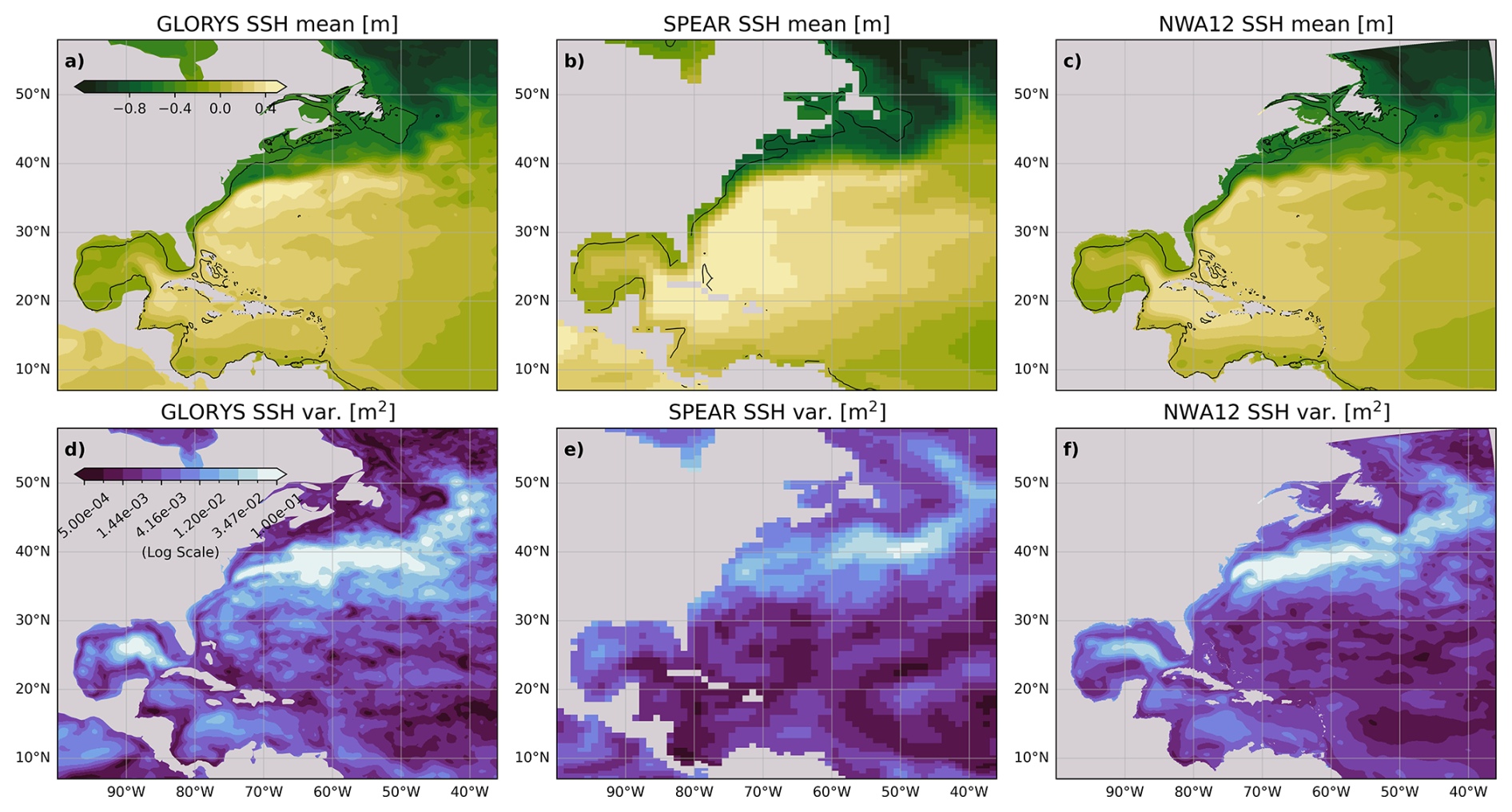
Figure 1 (a–c) GLORYS, SPEAR, and NWA12 1999 annual mean of daily average sea surface height (SSH) (GLORYS dynamic sea level is referenced such that the global mean is zero. This is used to initialize NWA12 SSH referenced to the model ellipsoid). The 150 m isobath is contoured in black. (d–f) GLORYS, SPEAR, and NWA12 1999 annual mean sea surface height variance (note log colorscale).

With the aim of improving simulations and, in the future, forecasts of sub-annual coastal sea levels, we leverage a recently developed dynamical downscaling framework to explore ocean and atmospheric influences along the US East Coast as they depend on model horizontal resolution. We focus particularly on the representation of daily extremes and their seasonal evolution, as well as the impact of model-resolved bathymetry along the continental shelf and slope margin. Our central focus is realized through comparison of retrospective forecasts, or hindcasts, of coastal sea level in a parent global atmosphere-ocean forecast model, the Seamless System for Prediction and Earth System Research (SPEAR) model (Delworth et al., 2020), and a higher horizontal resolution regional ocean model of the Northwest Atlantic (NWA12, Ross et al., 2023) forced at the boundaries by SPEAR. NWA12 realizes improved representation of shelf and slope circulation features (Fig. 1) and was developed as part of NOAA's Changing Ecosystem and Fisheries Initiative to drive a biogeochemical and ecosystem forecast model (Ross et al., 2024). We employ this downscaling framework for three purposes: to improve understanding of the processes that influence coastal sea level at sub-annual timescales, to determine ocean model horizontal resolution controls on the representation of coastal sea level variability, and to develop a framework for diagnosing time evolving coastal sea level distributions. We refrain from hindcast evaluation in terms of skill or error with respect to observed sea level at a given time, but rather consider model-dependent predictability associated with changing distributions (e.g. Sweet et al., 2022, 2024; Volkov et al., 2023) and focus on extremes that can adversely impact the built environment and put human lives at risk. If the time-varying nature of these distributions can be better understood and modeled, a more meaningful, useful, and accurate forecasting framework can be leveraged to save lives and property.

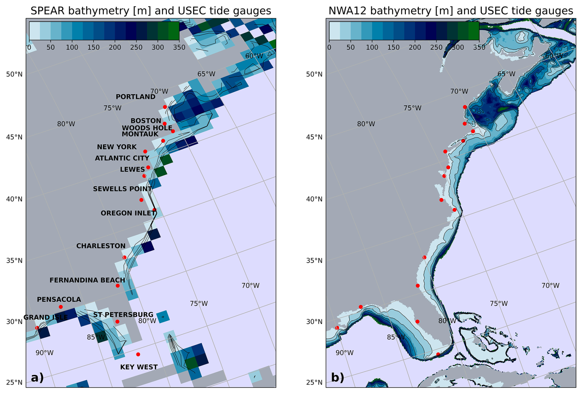
Figure 2 (a) SPEAR and (b) NWA12 continental shelf and slope bathymetry (0–350 m) colored at respective ocean model grid resolution. Black contours correspond to 25, 50, 100, and 150 m isobaths. Red dots locate the 15 tide gauge stations whose data are used in this analysis.

2 Configuration and methods

2.1 Parent model and downscaling configuration

We use the dynamical ocean downscaling framework developed in Ross et al. (2024) to downscale a suite of hindcasts from the global coupled SPEAR model. 1-year seasonal hindcasts from SPEAR, running in the medium resolution configuration with 0.5° atmosphere and 1° ocean resolution (Lu et al., 2020; Adcroft et al., 2019), were used as surface and ocean boundary conditions for 1-year simulations of the NWA12 regional ocean model. With $\mathrm{1}/\mathrm{12}$° ocean model resolution, NWA12 simulations have enhanced continental shelf and slope bathymetric resolution (Fig. 2), more realistic Gulf Stream representation (Fig. 1), and include tides (Ross et al., 2023, 2024).

For each initialization year, 1999–2018, five NWA12 ensemble member runs were carried out, with each member using a different ensemble member of the SPEAR hindcast as forcing. SPEAR ocean temperature, salinity, velocity, and sea surface height anomalies from each ensemble member were added to GLORYS12 reanalysis seasonal climatologies (Lellouche et al., 2021) to build ocean boundary forcings. This choice was made to permit ocean anomalies to cross NWA12 ocean domain boundaries and to ensure a smooth transition to interior NWA12 fields initially nudged using GLORYS12. As in Ross et al. (2024), daily-averaged SPEAR atmospheric fields of pressure, temperature, and humidity are interpolated from the 0.5° SPEAR atmospheric grid to the $\mathrm{1}/\mathrm{12}$° NWA12 grid and used as surface boundary conditions, with the exception of surface winds, which are updated at 6-hourly resolution. While surface ocean conditions do not feed back onto the atmosphere, wind stress calculations in NWA12 account for relative air-sea velocity, with NWA12 surface currents subtracted from the SPEAR surface winds.

Hindcasts were initialized on 1 December of each initialization year. Initial NWA12 ocean states were extracted from a 1993–2022 NWA12 run forced by ERA5 at the ocean surface (Hersbach et al., 2020) and GLORYS12 reanalysis climatology along ocean boundaries. In this 30-year run, interior temperatures and salinities were nudged toward concurrent GLORYS12 reanalysis monthly means. The December 1 initialization time was selected as SPEAR's large-scale seasonal predictions show the largest skill at this time due to enhanced predictive skill from the timing of the climatological ENSO cycles. 1 December also allows the simulations to capture the winter-spring transition, although the sensitivity of results to this choice was found to be low (excluding start times spanning the spring barrier). The resulting ensemble comprises five hindcast ensemble members initialized at the beginning of every December between 1999 and 2018 and run for one year, a total of 100 year-long simulations.

We acknowledge a missing feedback in the NWA12 ocean-only configuration in which the ocean currents and temperature in the regional model do not feed back onto the atmosphere in the forcing model. As a result, heat fluxes in NWA12 and SPEAR differ due to different ocean temperatures, but configurations and bulk formulae for the two are the same. For qualitative comparison to observations, it is also worth noting that SPEAR, along with many of the current seasonal prediction systems, exhibits bias in the magnitude and direction of near-surface winds (Delworth et al., 2020). Even so, and despite the decreased frequency at which the ocean-only model is forced by the atmosphere, we find enhanced NWA12 variability that we hypothesize arises partly as a result of winds acting on a higher-resolution ocean. This derives from the expectation that an enhanced response to the wind field should arise as ocean model resolution equals then exceeds atmospheric resolution. We also acknowledge that additional factors, for example, non-linear tide-current interactions, may contribute to enhanced NWA12 near-coast variance, but we expect these impacts to be smaller as NWA12 does not include a dynamic land/sea interface where these effects may become large.

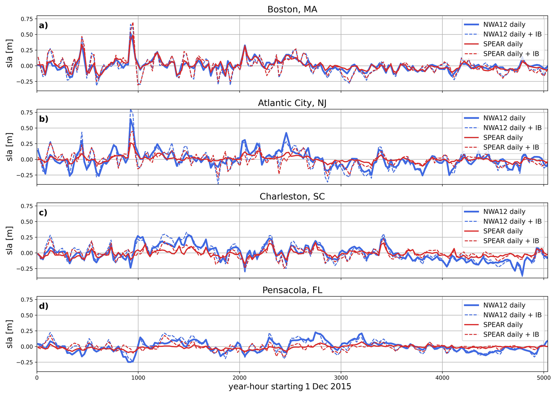
Figure 3 SPEAR (red) and NWA12 (blue) coastal sea level at Boston, MA (a), Atlantic City, NJ (b), Charleston, SC (c), and Pensacola, FL (d) tide gauge stations for the 1 December 2015–30 June 2016 period. Tides and a 20-year mean season cycle have been removed. Hourly non-tidal residuals in NWA12 are averaged in 24 h windows to obtain daily means. Solid and dashed lines are daily averages without and with the diagnosed IB contribution.

2.2 Analysis approach

Interrogation of these hindcasts focuses along the US East and Gulf Coast continental shelf, at fifteen long-established tide gauge stations with records generally greater than 75 years, and throughout the NWA12 domain at the surface. We quantify sea level variance: as a function of frequency using the discrete Fourier transform with a 12 h boxcar smoothing, within daily to monthly frequency bands using non-overlapping Butterworth filters, and at tide gauge stations through a thorough characterization of monthly distributions of daily sea level anomalies (SLA). Hourly coastal sea levels at tide gauge stations were also saved to enable comparison to hourly observations from the Global Extreme Sea Level Analysis (GESLA) dataset (Woodworth et al., 2016). Primary analyses focus on NWA12 comparison to SPEAR at daily and longer timescales. As SPEAR atmosphere and ocean fields were saved at daily resolution, this focus also enables offline assessment of inverted barometer (IB) effect contributions. In both NWA12 and SPEAR configurations, the ocean does not feel atmospheric pressure variations as computational limitations prohibit model timesteps from being short enough to resolve surface gravity waves. For output extracted at tide gauge stations, preprocessing began with removal of NWA12 prescribed tidal constituents using the utide Python library (Codiga, 2011). To enable appropriate comparison to SPEAR daily averages, hourly non-tidal residuals (NTRs) were then uniformly averaged across 24 h periods and centered at each mid-day time to generate daily timeseries (Fig. 3). A 1999–2018 mean seasonal cycle, calculated as the daily mean across all years and ensemble members for each day of the year was also removed.

As both SPEAR and NWA12 oceans were forced by the same surface wind field, we take particular focus on the ocean's near-coast response to onshore/offshore wind-driven transport. Daily surface wind stresses from SPEAR hindcasts were interpolated to the 150 m isobath and rotated and decomposed into local along and across isobath components. Connectivity between coastal sea level at tide gauge stations and along-shore winds was then considered at multiple coastal stations and across frequencies to reveal local and/or remote forcing and implied equatorward coastal wave propagation. The role played by the atmosphere, through wind and surface pressure forcing, is thus generally considered from variance contribution and regression perspectives, with model differences largely attributed to the representation of continental shelf dynamics and its areal extent over which wind stresses can act. We acknowledge that shelf sea level changes reflect both local mass and density changes, but avoid decomposition into components as our primary focus is at the coast where the density contribution vanishes. The role of wind- or circulation- driven cross-shore mass transport over the shelf across daily to monthly timescales will depend on shelf representation, but as shelf depths are very shallow compared to those offshore, we expect little density contribution differences between the two models.

In focusing on horizontal resolution importance for coastal extreme representation, we lastly consider SPEAR, NWA12, and observation-derived monthly distributions of deseasonalized daily sea level anomalies. 5th and 95th percentile values are calculated for each month at each tide gauge station. The role of the IB effect in shaping these distributions is separately considered in comparison to observed timeseries, spectra, and daily distributions. While both SPEAR and NWA12 oceans do not feel atmospheric pressure variations, the IB effect is calculated offline (Ponte, 2006) and added to simulated coastal sea level for comparison to observations that include pressure effects. In using daily mean surface pressures, referenced to global ocean mean, higher frequency variability associated with synoptic scale storms may result in an underestimation of extremes and distribution tails. Comparisons between SPEAR and NWA12, however, isolate the effect of improved shelf and slope process representation and response to surface forcings.

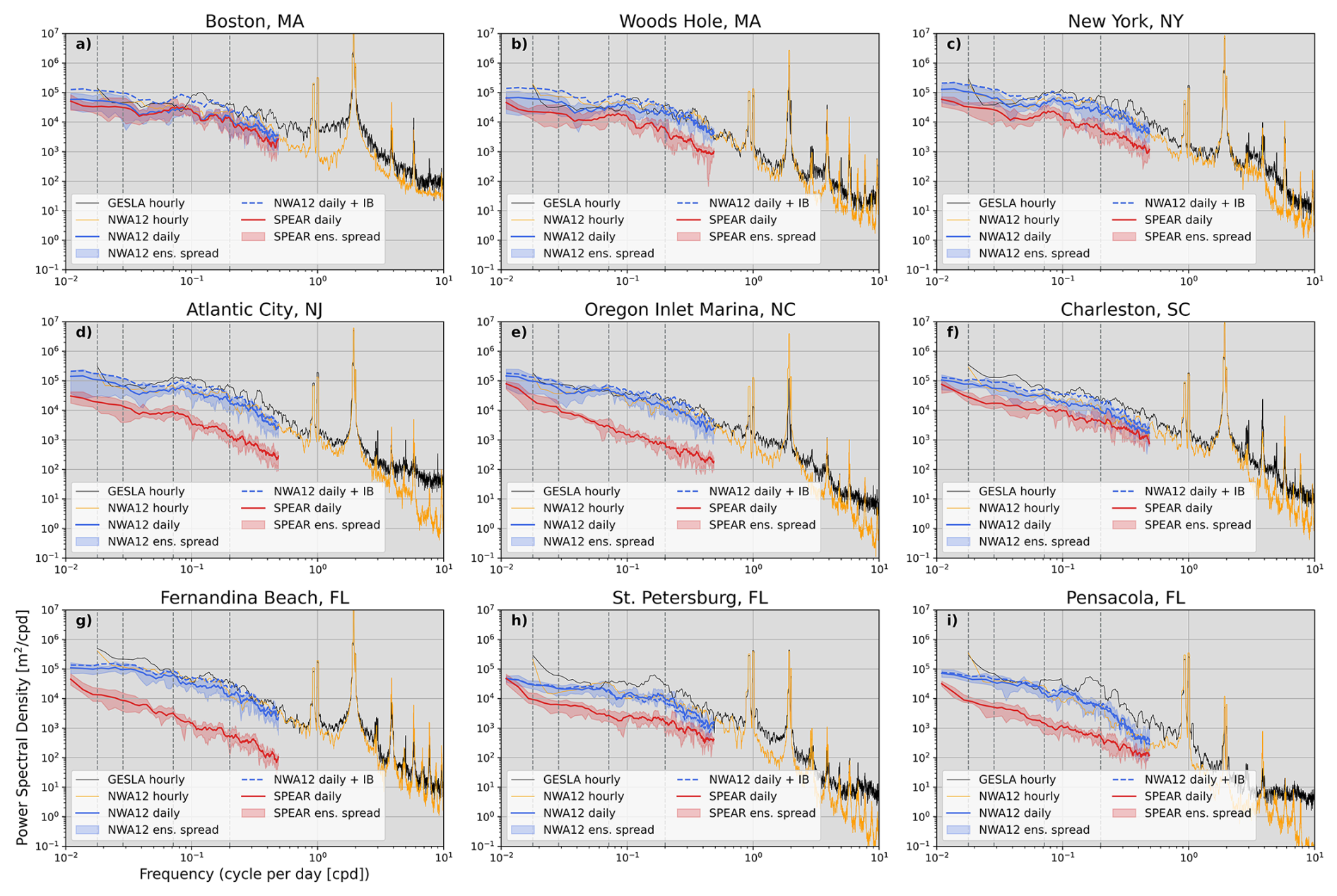
Figure 4 Power spectral density at nine tide gauge stations. Black denotes observed and yellow NWA12 hourly spectra for the 1 December 2018 simulation start time. Solid red (SPEAR) and blue (NWA12) are ensemble-mean daily spectra with the blue dashed line adding the IB contribution. Red and blue shading encompass the ensemble spread. Moving left to right, light gray vertical dashed lines correspond to 2-month, 1-month, 2-week, and 5 d periods.

3 Results and discussion

3.1 Frequency spectra at tide gauge stations

Initial comparison between SPEAR and NWA12 at tide gauge stations reveals a SPEAR-NWA12 difference in variance across daily to monthly frequencies that is a strong function of latitude (Figs. 3 and 4 – red vs. blue curves). At the Boston tide gauge station, SPEAR and NWA12 have comparable energy across resolved frequencies, similar to the observed spectrum, but moving south along the coast through the Mid-Atlantic and South-Atlantic bights (MAB and SAB, respectively), SPEAR variance reduces by nearly an order of magnitude compared to both NWA12 and observations. The IB contribution to sea level variability is greatest at higher latitudes (∼ 33 %, Piecuch and Ponte, 2015) and decreases to the south (Figs. 3 and  4 dashed lines). This pattern reveals a modest contribution of extratropical storms on sea level variability that diminishes at stations located further away from the climatological position of the mid-latitude storm track, a feature generally well resolved by SPEAR (Lee et al., 2025). Across hourly to daily frequencies, NWA12 spectra compare favorably with observations at all stations. This suggests tides are well resolved and lends support to the argument that this dynamical downscaling framework improves the representation of coastal and shelf dynamics.

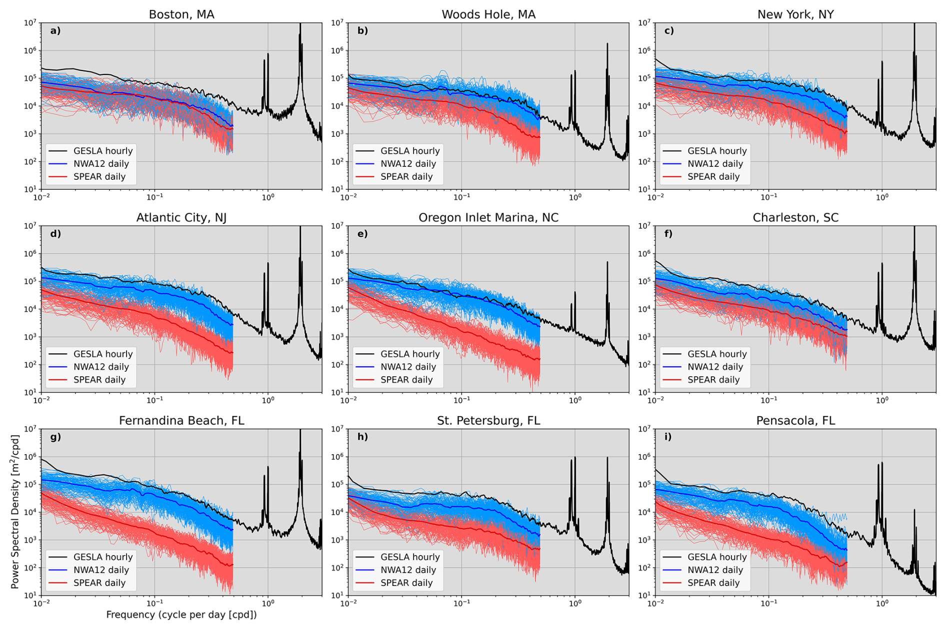
Figure 5 SPEAR (red) and NWA12 (blue) daily-mean power spectral density curves at nine tide gauge stations. Averages across twenty initialization years and ensemble members are added as thicker red and blue curves. Twenty-year mean spectra computed from hourly observations is added in black.

The SPEAR decrease of energy with decreasing latitude is apparent in all 1-year simulations and across all ensemble members (Fig. 5). While the full NWA12 ensemble mean is still less energetic than GESLA at most sites, NWA12 variability across daily and lower frequencies is much closer to observations than SPEAR, especially within and south of the MAB. Across these frequencies SPEAR and NWA12 ensemble spreads minimally overlap suggesting distinct improvement. These differences between SPEAR and NWA12 span a range of frequencies including those which SPEAR is expected to resolve, as well as those associated with processes unexpected to be resolved by SPEAR due to its relatively coarse shelf resolution. These include higher frequency motions like coastal trapped waves that require a wide shelf and well-resolved cross-shelf bathymetric gradient. Absence of these bathymetric features (Fig. 2) suggests a limited pathway for along-coast signal propagation, especially across the narrowest point near Cape Hatteras.

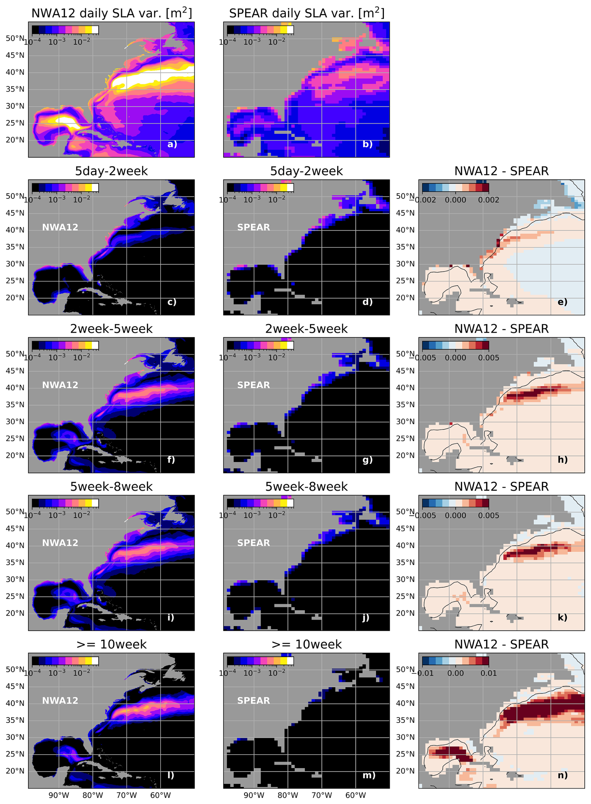
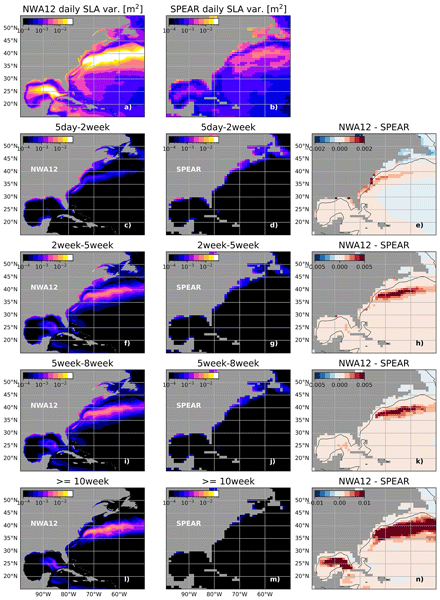
Figure 6 (a, b) Deseasonalized total SPEAR and NWA12 sea level anomaly (SLA) variance. Variance is partitioned into four frequency bands (5 d–2 week (c, d), 2 week–5 week (f, g), 5 week–8 week (i, j), and greater than 10 weeks. (e, h, k, and n) Differences in variance (NWA12 – SPEAR) at SPEAR horizontal resolution.)

3.2 Band-passed variance

To assess sea level variability as a function of frequency throughout the model domain, deseasonalized daily sea level anomalies were band-pass filtered to partition variance into four bins: 5 d to 2-week, 2-week to 5-week, 5-week to 8-week, and greater than 10 weeks. These bands were selected to partition variance across weather to seasonal timescales, the full span of resolved frequencies from these 1-year simulations. The 5 d to 2-week band was selected to contain variability linked to synoptic scale weather, while the others capture a range of sub-seasonal atmosphere and ocean variability. Importantly, this separation includes frequencies expected to be well resolved by both SPEAR and NWA12 and frequencies that only NWA12 can resolve associated with tides and dynamics permitted due to higher horizontal resolution. Resulting variance at each NWA12 grid point and within each frequency bin was then averaged across adjacent grid points to smooth NWA12's $\mathrm{1}/\mathrm{12}$° degree horizontal resolution to the SPEAR 1° resolution and enable difference maps to be generated (Fig. 6). These maps reveal geographically a difference in dominant timescales of variability along the coast and offshore. Along the MAB, SAB, and Gulf coasts, variability in the 5 d to 2-week band is over one order of magnitude greater in NWA12 than in SPEAR. Along the northeast coast within the Gulf of Maine, however, the SPEAR model's variance in this bin is slightly greater than NWA12. Within all lower frequency bins, NWA12 sea level variance is over an order of magnitude greater than SPEAR away from the coast and within the Gulf Stream and Loop Current. This added energy can be partly attributed to NWA12's finer horizontal resolution that enables a more realistic representation of mesoscale eddy turbulence.

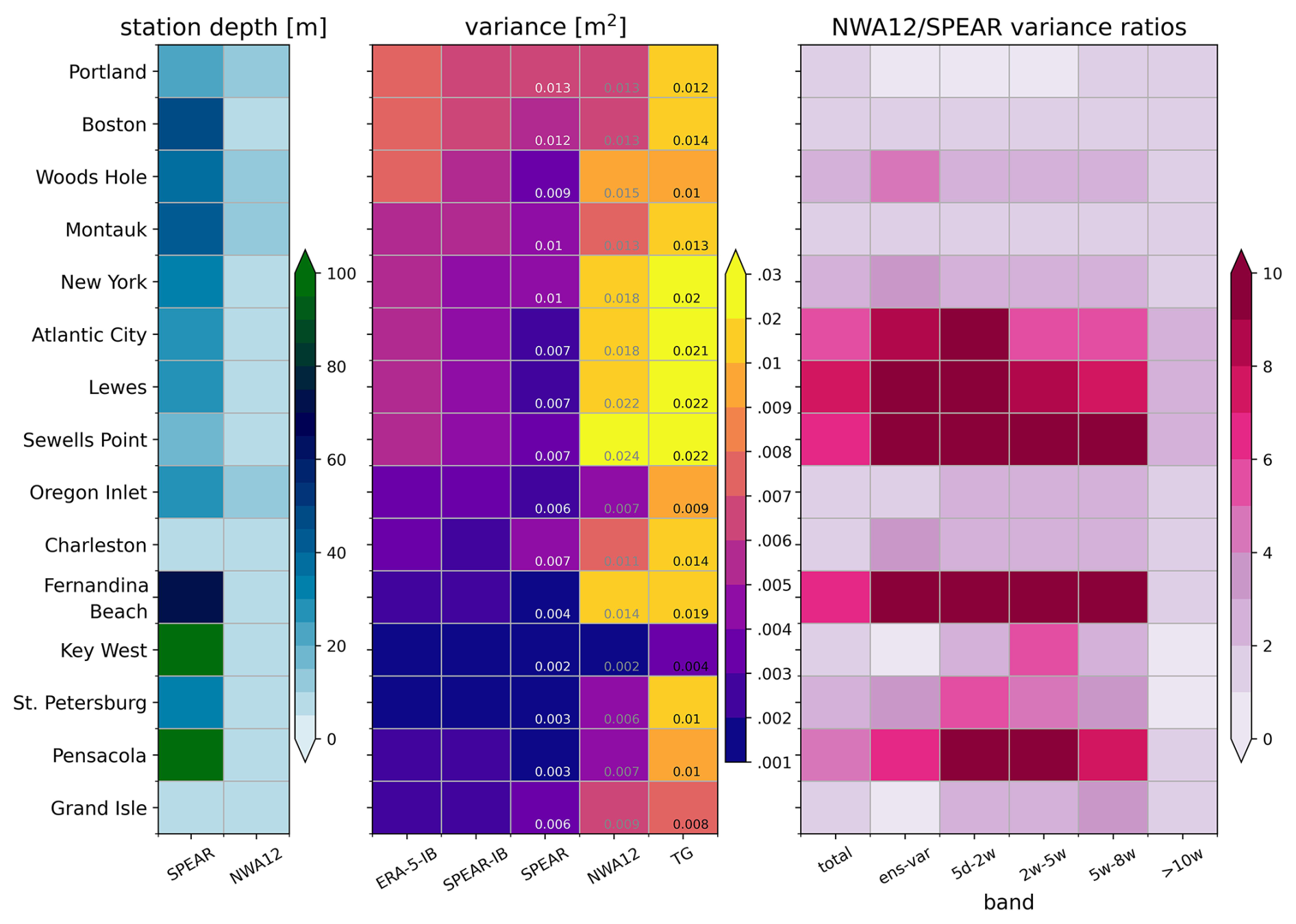
Figure 7 (left) SPEAR and NWA12 ocean depth at 15 tide gauge stations. (middle) Coastal sea level variance: ERA-5 inverted barometer contribution (ERA-5-IB), SPEAR inverted barometer contribution (SPEAR-IB), SPEAR, NWA12, tide gauge observations (TG). Text reports model sea level variance with the IB contribution included and observed sea level variance. Note colormap and colorbar are on a log scale. (right) NWA12/SPEAR variance ratios: total, ensemble spread (ens-var), and for each frequency bands.

At the fifteen tide gauge stations considered here, SPEAR and NWA12 variance differences are explored more closely and alongside station depth differences and observed variance (Fig. 7). At nearly all stations, coastline-adjacent NWA12 grid cells are shallower that those in SPEAR (Fig. 7, left). These differences, greatest north of Cape Hatteras and along the Florida coastline, contribute to a decrease in SPEAR coastal sea level variance arising from less coastal amplification or shoaling. Diagnosed IB contributions compare favorably to reanalyses and when added to model coastal sea level variance, NWA12 values approach observed values (Fig. 7, middle). Ratios of NWA12 to SPEAR variance (Fig. 7, right) reveal a five-fold or greater increase in coastal sea level variance in this region that is largely constrained to shorter timescales. Further north, SPEAR and NWA12 stations show comparable variance suggesting more limited downscaling improvements in this region. South of Cape Hatteras, NWA12 increases appear linked to coastal station depth differences. These comparisons reveal the extent and pattern of NWA12 coastal variance increases and show that they approach and better match observed values.

3.3 Connections to relevant dynamics: wind stress and boundary currents

Sea level variability along continental shelves can be significantly influenced by local and remote along-shore winds driving across-shore Ekman transport and exciting coastal trapped waves (Wang et al., 2022). Along the US East Coast, winds are predominantly northwesterly and typically strongest in the winter, becoming light and variable in the summer. After removing a seasonal climatology to highlight a coastal sea level response to wind anomalies across daily to weekly timescales, daily SPEAR along-shore wind stress anomalies are regressed onto coastal sea level anomalies at Atlantic City, NJ, and Charleston, SC. This approach was adopted to reveal the spatial pattern and strength of a main driver of coastal sea level variability. As both SPEAR and NWA12 oceans see the same atmosphere, before calculation of relative wind stress, comparisons reveal differing coastal sea level response patterns to wind stress anomalies over the shelf that, while dependent on timescale, suggest the importance of continental shelf resolution.

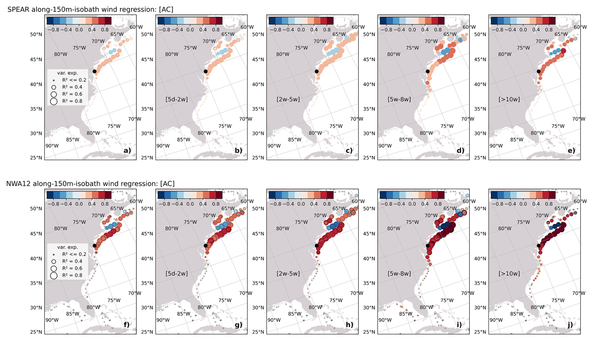
Figure 8 Regression of along-150 m isobath winds with SPEAR total SLA at Atlantic City, NJ (black-circle) (a) and as a function of frequency band (b–e). (f–j) Same as (a–e) but for NWA12. Colored circle size corresponds to the fraction of variance explained by along-isobath winds. In (f–j), the open black circles are the fraction of variance explained in (a–e).

This connectivity is assessed first at Atlantic City. North of Cape Hatteras, NWA12 regression coefficient magnitudes are larger than those in SPEAR by nearly a factor of two (Fig. 8, correlations also approximately double - not shown). This increase can be at least partly attributed to the improved representation of the Mid-Atlantic and New England continental shelf bathymetry (Fig. 2). Regression values are greatest between Georges Bank and New Jersey, suggesting this region to be a runway for along-shore wave generation/propagation and the setup of an along-shore pressure gradient. Where these NWA12 regression coefficients are elevated, the fraction of coastal sea level variance explained increases relative to SPEAR by 10 %–20 % (size of colored circles in Fig. 8). This increase is largest in the 5 d to 2-week band and at longer timescales SPEAR and NWA12 fractions are comparable. Lentz (2024) discusses these factors in detail and shows that a simple wind-driven depth-average model configured for this section of continental shelf can well reproduce coastal variability. Regression coefficient magnitudes in this region are elevated within all frequency bands. Magnitudes south of Cape Hatteras, however, marginally increase only within the lowest frequency band, suggesting the large-scale wind field, which varies at these multi-month timescales, imprints on this metric, as there is no poleward signal propagation pathway. This inference is consistent with a comparison of correlation coefficients between along-shore wind stress values offshore of Charleston and Atlantic City. Correlations are weak, but increase at timescales greater than ∼ 2 weeks.

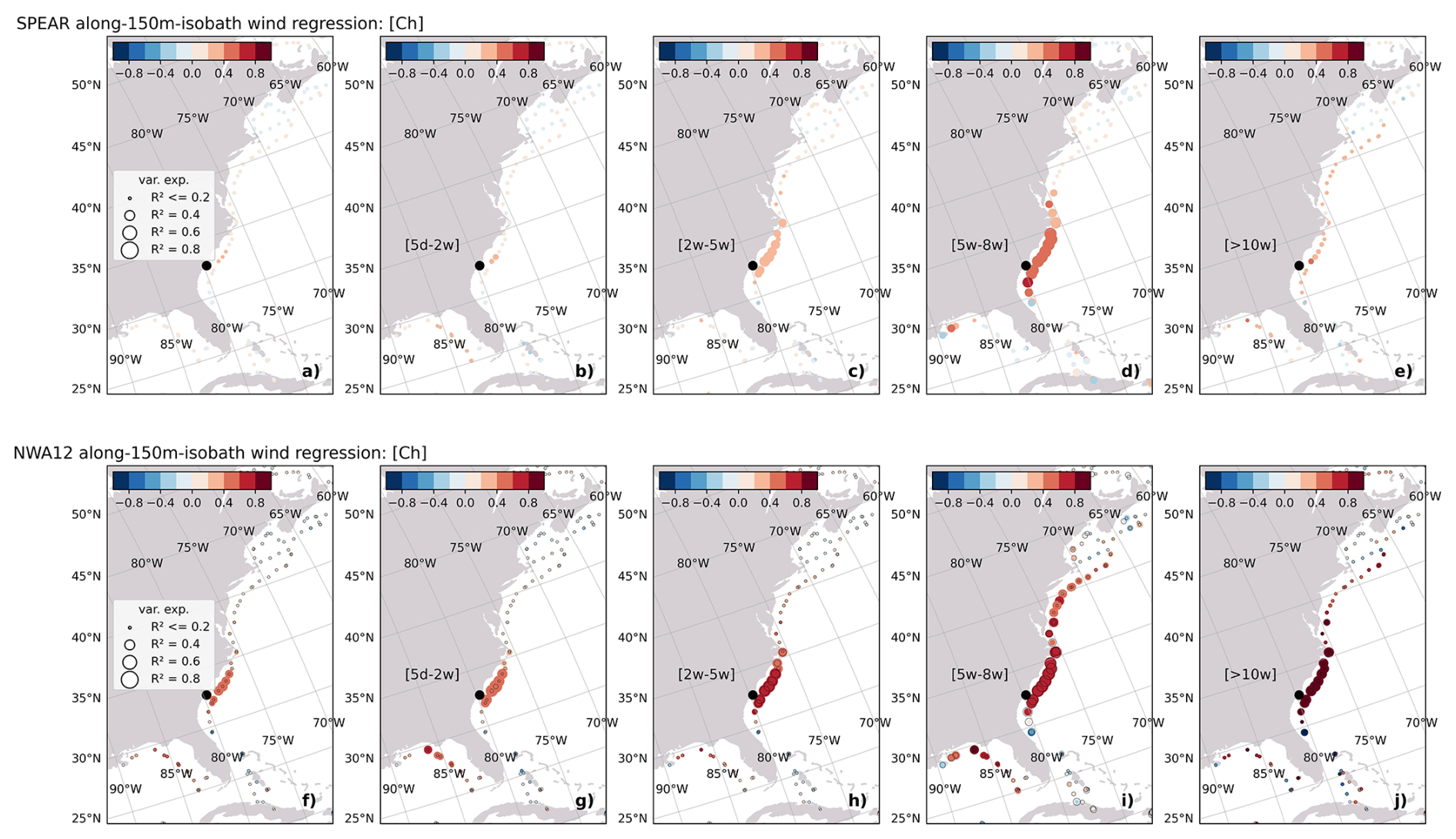
Figure 9 Same as in Fig. 8, but for Charleston, SC.

South of Cape Hatteras, at Charleston, wind stress anomaly regression coefficients and fraction of variance explained are also elevated in NWA12 compared to SPEAR (Fig. 9). The most significant increases in fraction of variance explained, over 25 %, occur in the SAB in the 5 d to 2-week band and in the MAB in the 5-week to 8-week band. In NWA12, this shift to the MAB with increasing timescale suggests, as in Little et al. (2026), connectivity across Cape Hatteras that is limited or absent in SPEAR due to model horizontal resolution. This agrees with the expectation of equator-ward propagation of coastal waves, but also the increasing spatial scale of lower frequency wind variability. As at Atlantic City, these increased regression coefficient magnitudes in NWA12 suggest increased sensitivity to along-shore wind stress that is linked to continental shelf representation.

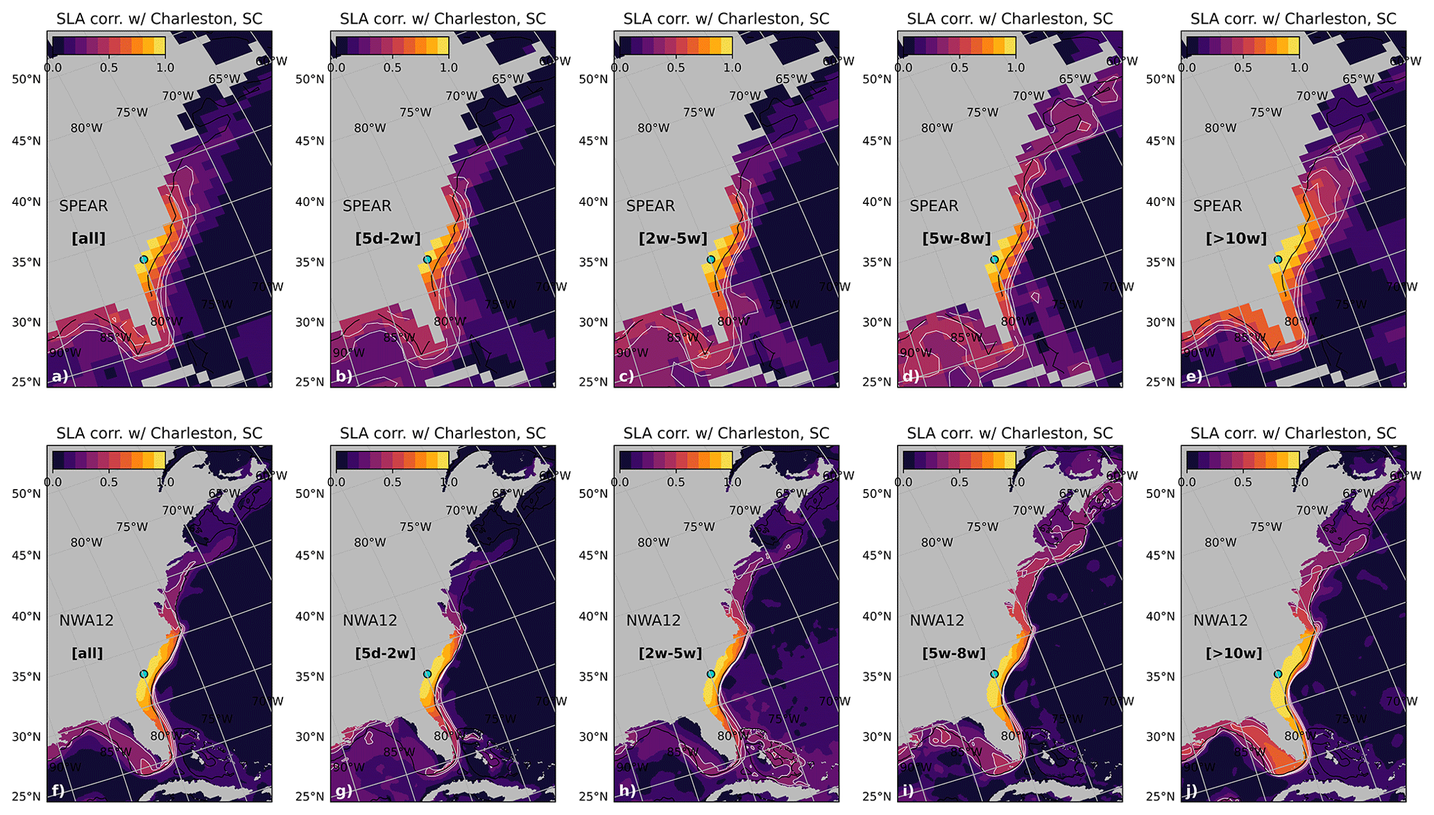
Figure 10 SPEAR (a–e) and NWA12 (f–j) SLA correlation with SLA at the Charleston, SC tide gauge station. Panels (a) and (f) are correlations with the full timeseries, (b) and (g) within the 5 d to 2-week band, (c) and (h) within the 2-week to 5-week band, (d) and (i) within the 5-week to 8-week band, and (e) and (j) for timescales longer than 10 weeks. Black contour is the 150 m isobath.

Along the western boundary of the major ocean basins, coastal sea level is also influenced by the position and strength of western boundary currents. The poleward-flowing Gulf Stream and subsurface intensified equator-ward flowing slope current exert both local and remote effects on US East Coast sea level (Ezer, 2016; Camargo et al., 2025). Together, this western boundary current variability reflects changes in the Atlantic Meridional Overturning Circulation and lower frequency coastal sea level variations (Yin et al., 2009; Little et al., 2019). At higher frequencies, flooding events have been linked to the AMOC state (Volkov et al., 2023), but more locally, the Gulf Stream extension position and along-coast jet strength (Donatelli et al., 2025). Connectivity, or lack thereof, between slope or offshore variability and the coast also depends strongly on the bathymetric resolution of the shelf and slope. A significant difference between NWA12 and SPEAR to this effect appears in the pattern of correlation of coastal sea level at Charleston and sea surface height throughout the region (Fig. 10). Within the lowest frequency band considered, at timescales of Gulf Stream position changes, SPEAR correlations are broadly elevated offshore of the shelf-slope transition, while elevated NWA12 correlations are confined to the inner shelf (Fig. 10e and j). This suggests potentially undesired elevated Charleston sea level sensitivity in SPEAR linked to offshore Gulf Stream behavior. In NWA12, elevated correlations appear more tightly confined to the SAB shelf, along the slope, and at the point of Gulf Stream detachment from the coast.

While SPEAR ocean horizontal resolution is too coarse to resolve the first baroclinic Rossby radius of deformation over the continental shelf (𝒪 2–10 km), and NWA12 may at best resolve this radius with one grid cell, model resolutions relative to the shelf width are quite different. SPEAR may resolve the average US east coast shelf width of 100–150 km with one grid cell while NWA12 will have over twelve. Where the shelf narrows, coastal grid cells in SPEAR will generally be too deep as they are generated by averaging over shelf and slope depths. These differences impact shelf process and coastal trapped wave representation significantly and reveals where dynamical downscaling will improve model coastal sea level.

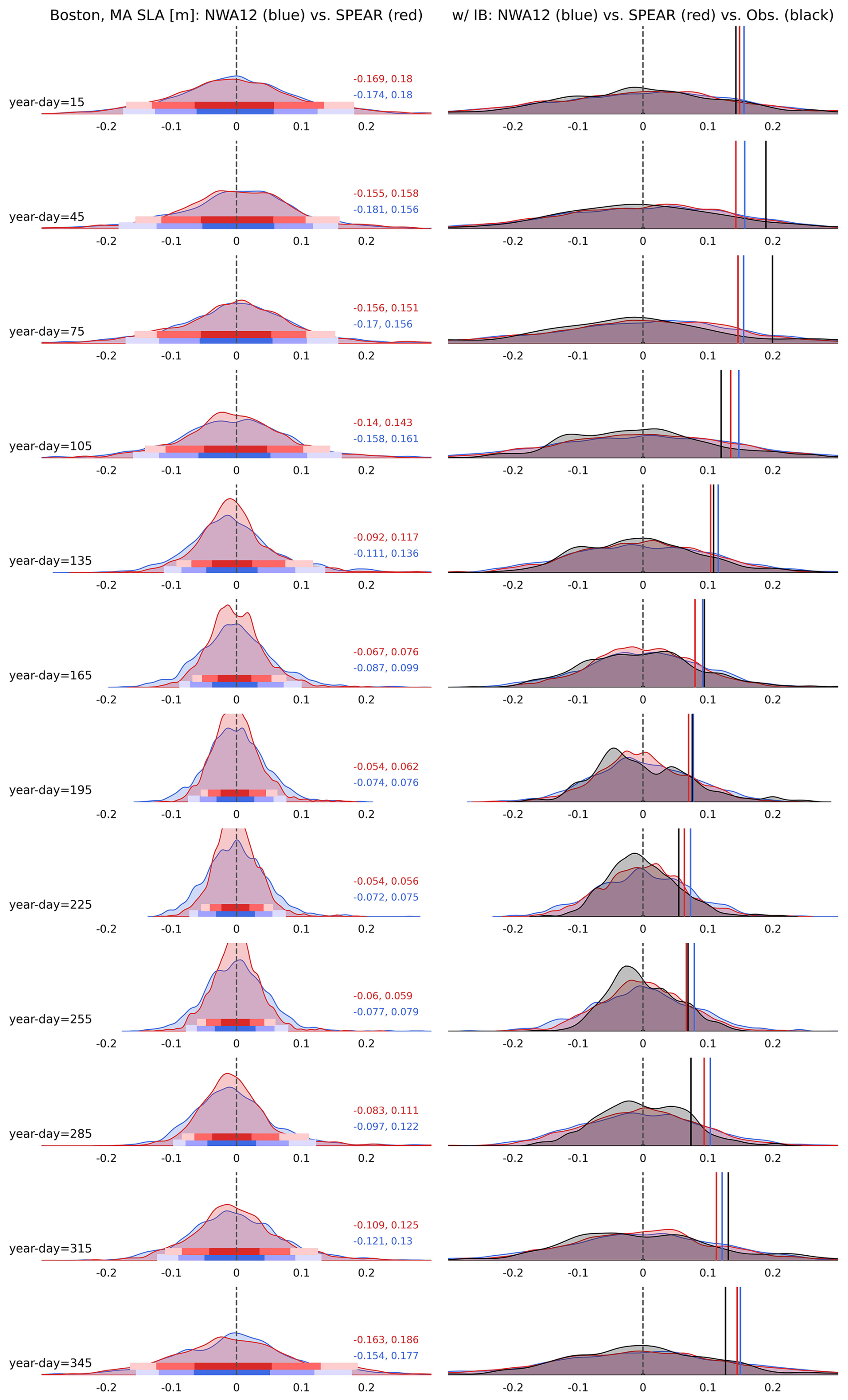
Figure 11 (left) Distributions of daily SPEAR (red) and NWA12 (blue) SLA at the Boston, MA tide gauge station as a function of lead month. Horizontal bands denote 5, 10, 25, 75, 90, 95 percentiles. Red and blue text are 5th and 95th percentile values for SPEAR and NWA12. (right) Distributions of daily SPEAR (red), NWA12 (blue), and observations (black) with the IB effect included. Solid vertical lines denote corresponding standard deviations.

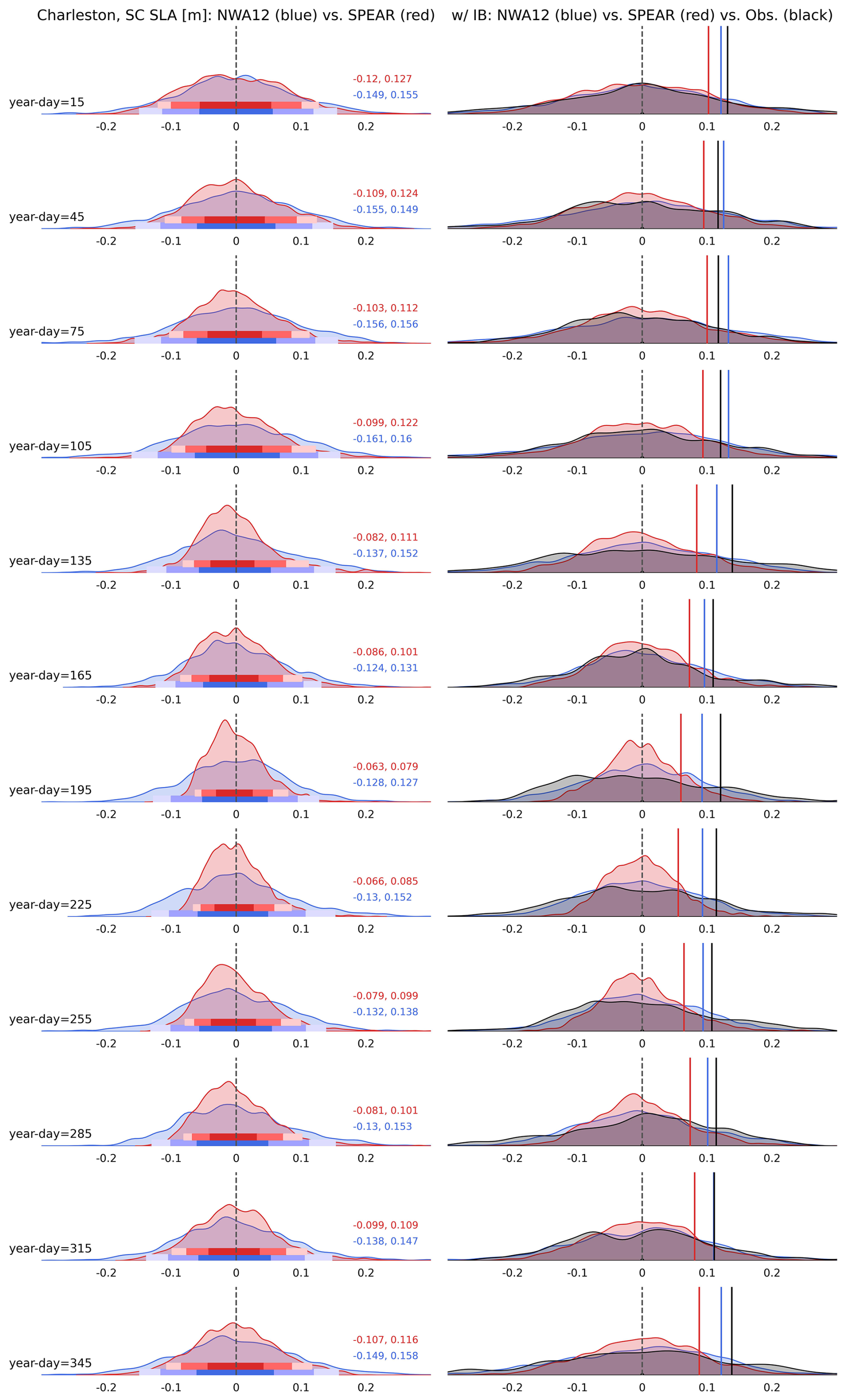
Figure 12 (left) Distributions of daily SPEAR (red) and NWA12 (blue) SLA at the Charleston, SC tide gauge station as a function of lead month. Horizontal bands denote 5, 10, 25, 75, 90, 95 percentiles. Red and blue text are 5th and 95th percentile values for SPEAR and NWA12. (right) Distributions of daily SPEAR (red), NWA12 (blue), and observations (black) with the IB effect included. Solid vertical lines denote corresponding standard deviations.

3.4 Seasonality of daily distributions and extreme events

These different process representations and responses to surface forcings also impact the magnitude and occurrence of daily extremes. Metrics such as frequency of occurrence, extreme event likelihood, or rate of return all derive from distribution characterizations that vary in space and time, but if properly assessed, reveal sources of predictability. Ensemble-mean NWA12 and SPEAR distributions of daily coastal sea levels, binned by simulation lead month and with a climatological seasonal cycle removed, are considered at all tide gauge stations. Distribution shape and width are first evaluated at two tide gauge stations, Boston, MA (Fig. 11) and Charleston, SC (Fig. 12). At Boston, distribution evolution reveals a seasonal cycle, decreasing in width through the summer and widening throughout the winter. With the IB effect added to facilitate NWA12 and SPEAR comparison to observations, this seasonal cycle is realized as a two-fold change in distribution standard deviation. At Charleston, this seasonal cycle in distribution width is muted, with SPEAR over-representing a narrowing throughout the summer. NWA12 distributions remain wider throughout the year, a pattern more similar to observations and likely linked to coastal wave and Gulf Stream variability. At all stations, model extremes, and distribution tails, are expected to be under-represented as daily mean surface pressures miss a higher-frequency component of coastal flooding and surge associated with synoptic storms.

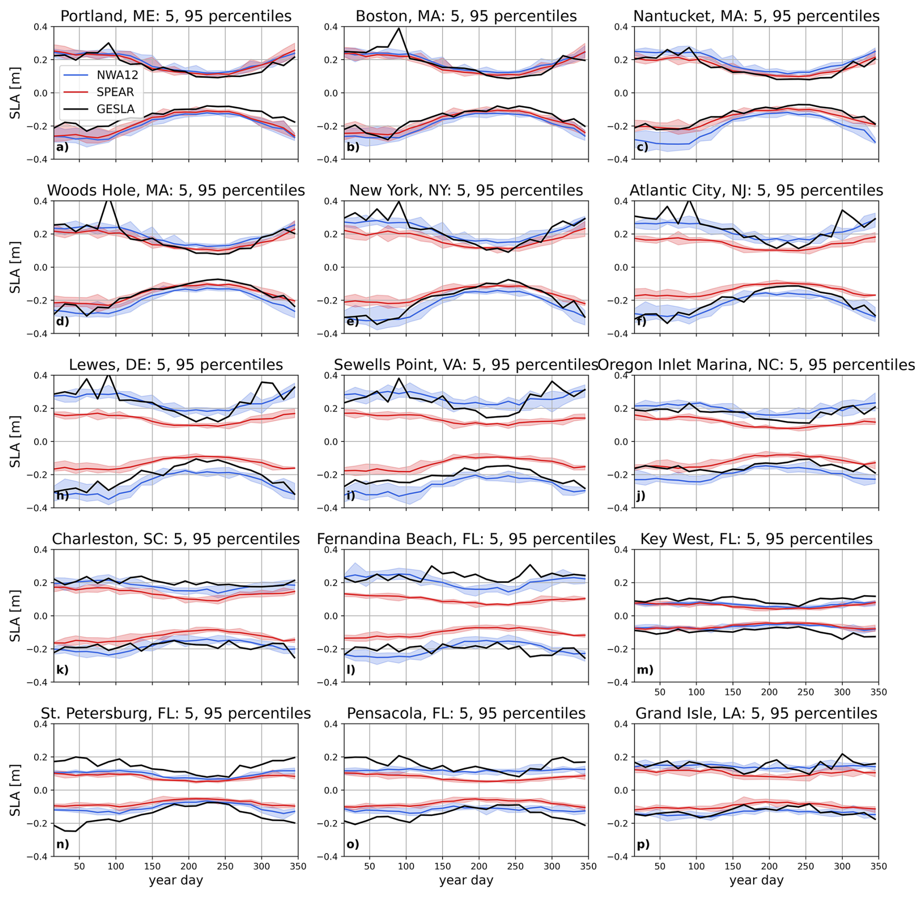
Figure 13 5th and 9th percentiles of daily sea level anomaly distributions as a function of simulation lead time (days since model initialization). SPEAR is in red, NWA12 in blue, and observations (GESLA) in black. Red and blue shading shows the mean ensemble spread.

Distributions are further characterized by constructing a climatology of ensemble-mean 5th and 95th percentiles (Fig. 13). As suggested by differences between Boston and Charleston, this characterization reveals a latitudinal dependence of the seasonal cycle of distribution width and extreme occurrences. Along the New England and mid-Atlantic coasts, 5th and 95th percentile values increase through the winter and decrease during the summer. This seasonal cycle is well represented in NWA12 and SPEAR at the northernmost tide gauges, but moving south, into the MAB, SPEAR extreme amplitudes notably decrease. South of Cape Hatteras, distributions exhibit a damped seasonal cycle, but NWA12 consistently resolves larger 5th and 95th percentile values, especially in the SAB. Ensemble member spread, shaded bands in Fig. 13, reveal consistency in these NWA12-SPEAR differences.

Together, these characterizations of daily distributions of coastal sea level reveal a latitudinal dependence on the strength and representation of a seasonal cycle in daily extremes. At higher latitudes, the SPEAR and NWA12 distribution shapes and seasonal evolutions align with observations. Here, distribution width increases in the winter, associated with increased extra-tropical storm activity, and extremes become larger in magnitude. Moving south into the MAB, SPEAR distributions narrow and exhibit a relatively weaker seasonal change in width as compared to NWA12 and observations. As winds in NWA12 and SPEAR are identical, we attribute this decreased variability to the limited resolution of the Mid-Atlantic and New England continental shelves. Without a well-resolved shelf, with depths increasing with distance offshore, equator-ward propagating waves are poorly resolved. Further south, along the SAB and Gulf Coasts, the seasonal cycle weakens in both models and observations, but extreme magnitudes are over 50 % greater in NWA12 at most stations.

4 Conclusions

In this analysis, we leverage a recently developed dynamical downscaling framework to generate high-resolution year-long hindcasts of US East Coast sea level. A 100-member ensemble is built to explore patterns of variability and assess the structure and evolution of daily coastal sea level distributions. Downscaled regional (NWA12) and parent global (SPEAR) model hindcast differences are considered throughout the downscaled domain and high-frequency model output is compared to coastal sea levels at tide gauge stations. While we acknowledge that model configuration differences contribute to differences in coastal process representation, we focus on and contrast NWA12 and SPEAR coastal sea level variability linked to continental shelf and slope representations. From a coastal sea level perspective, these results highlight the importance of resolving coastal and ocean basin margin dynamics, including western boundary currents.

Monthly distributions of daily coastal sea levels differ significantly in downscaled and parent model output. Distributions across all months are wider in NWA12, reflecting the enhanced representation of short-term extremes. While these distributions are determined after removal of a monthly seasonal climatology from coastal station time series, they exhibit a seasonal cycle with location dependent amplitudes. At northern tide gauge stations, NWA12, SPEAR, and observed distributions are similar across all months, but moving south, SPEAR distributions become excessively narrow, especially in summer months. These differences also manifest away from the coast. Throughout the NWA12 domain, the relationship between model horizontal resolution and sea level variability appears influenced by continental shelf and slope structure as well as adjacent boundary current representation. As in Li et al. (2022), Volkov et al. (2023), Zhang et al. (2025), and Little et al. (2026), we link horizontal resolution increases with the improved representation of shelf and slope dynamics.

In a general sense, near-coast and open-ocean co-variability depends on continental shelf hypsometry and width. Where the shelf is relatively wide and shelf-break sharp, strong cross-shore potential vorticity and bathymetry gradients act to insulate the coast. A model's ability to well simulate coastal sea level is then closely tied to the representation of this open-ocean to coastal dynamical transition. In this work, we find NWA12-SPEAR differences to vary significantly with latitude. As both model oceans feel the same atmosphere, but different relative winds whose strength generally increases with latitude, these differences are partly attributed to differing coastal station depths and resolution-dependent ability of along-shore winds to excite cross-shore transport and along-shore waves. Shelf bathymetric resolution is thus recognized as a central control on the realistic simulation of coastal sea level. Little et al. (2026) identify Cape Hatteras, NC as an important `choke point' where continental shelf width decreases substantially. If model resolution cannot resolve this segment along the coastal wave guide, downstream coastal sea level variability will be muted. Compared to NWA12 and observations, we find such decreased SAB variability in SPEAR that is further associated with limited representation of the Gulf Stream and its imprint along the coast (Donatelli et al., 2025).

Overall, this analysis demonstrates that dynamically downscaled hindcasts yield more realistic simulations of US East Coast sea level variability across daily to monthly timescales. While the nature and magnitude of this enhanced variability varies geographically, with enhancements generally greater at lower latitudes, daily distributions of downscaled output exhibit temporal variability, width, and extremes that more closely align with observations at all tide gauge stations. With these improvements, contextualized alongside recent results that explore distribution shape evolution (Hovenga et al., 2025), datum re-assessment (Piecuch et al., 2025; Gregory et al., 2019), and extreme events as they impact the built environment (Maghsoodifar et al., 2025), this framework can be further leveraged and applied in a true forecasting sense to generate more locally relevant information built on mechanistic understanding. Next steps focused on generating statistics-oriented forecasts that can be used in applied settings are deemed feasible as SPEAR seasonal forecasts are generated seasonally, bias correction is not needed as ocean anomalies are applied to climatology, and single ensemble member NWA12 run times are only a few hours. For single year forecasts, we plan to generate a larger ensemble to enhance statistical robustness. Five ensemble members were chosen here to focus on parent and downscaled model differences relative to internal variability. Together, these continued efforts aim to improve preparedness for realized and future higher frequency flooding hazard risk changes (Qu et al., 2026).

In comparing downscaled and parent ocean model output forced by the same atmosphere, we highlight the link between representation of shelf and slope ocean dynamics and coastal sea level variability. We explore this link in terms of ocean model sensitivity to along-shore wind stress and the representation of ocean boundary currents. Our results highlight the importance of resolving shelf bathymetry, but also help develop interpretability of larger scale forecasts of climate variability in their application to local coastal changes and their physical drivers. As the occurrence and intensity of extreme events changes at monthly and longer timescales (Xu et al., 2026), the distributional characterization and linkage to model resolution discussed here further connect forecast output to process representation. In this context and with this tool, sub-annual coastal sea level variability can be better understood and predicted to mitigate risks to life and property.