Diapycnal mixing in submesoscale-permitting simulations of the deep Brazil Basin

Modeling diapycnal mixing in the deep ocean is challenging, particularly in regions with complex topography. Here we diagnose the relative roles of sub-inertial motions and tidal forcing focusing on the deep Brazil Basin in simulations using a hydrostatic, high-resolution regional model (CROCO) at 1, 3 and 6 km horizontal resolution, in presence or absence of tides. Tracer particles are released at multiple depths to investigate the variability of modeled mixing estimates. Horizontal resolution exerts the primary control on diapycnal mixing, while tidal forcing plays a secondary and resolution-dependent role. Increasing resolution significantly increases the number and intensity of eddies and enhances diapycnal mixing across the water column, from the bottom to at least 3000 m. The comparison with the in-situ observations indicates that the simulated diffusivities near the bottom boundary layer are comparable in value to observational estimates in the 1 and 3 km cases and too small in the 6 km run. However, diffusivities in the stratified interior are overestimated and the model-observation discrepancy grows for increasing resolution. At submesoscale-permitting resolutions, due to bathymetric smoothing, high-mode internal tides remain significantly underestimated, while submesoscale eddy-driven motions are overrepresented, leading to the biased estimate of diapycnal mixing.

1 Introduction

In the ocean, diapycnal mixing governs the vertical exchange of mass, heat, salt, and tracers across density surfaces, thereby controlling ocean stratification. Through irreversible turbulent fluxes, diapycnal mixing provides also the mechanical energy dissipation required to sustain the upwelling branch of the overturning circulation (Ferrari et al., 2016; Polzin and McDougall, 2022). Although background mixing rates in the ocean interior are weak, observations consistently show that strongly localized enhancements near rough topography dominate the net diapycnal transport and water mass transformation (Polzin et al., 1997; Ledwell et al., 2000). Multiple mechanisms contribute to topographically enhanced mixing, including internal hydraulic jumps (Legg and Klymak, 2008), Ekman layer processes (Garrett et al., 1993), internal wave generation and breaking (Wunsch and Ferrari, 2004), vertically sheared layered vortices (Mashayek et al., 2024), and overturning instabilities (McWilliams, 2016).

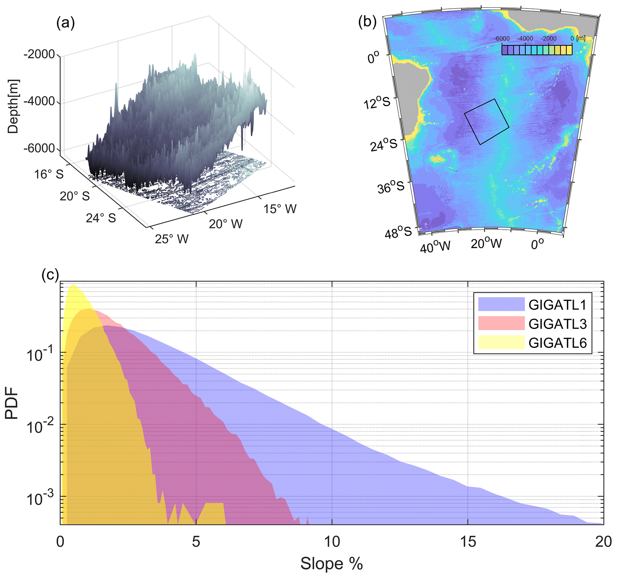
Figure 1 Study region and context in the abyssal Brazil Basin. (a) The bathymetry of the model study region. (b) Map of the Brazil Basin showing the model study region (black box). (c) Probability density function of slope distribution of GIGATL1 (1 km resolution), GIGATL3 (3 km resolution) and GIGATL6 (6 km resolution) simulations in the black box.

The efficiency of topographic mixing depends sensitively on regional circulation and bathymetric detail, and thus, in ocean models, on model resolution. While increasing computational power now permits global and basin-scale simulations at mesoscale-resolving and even submesoscale-permitting resolution, these models often produce counterintuitive diapycnal mixing relative to coarser configurations, largely because they retain vertical mixing parameterizations developed for much lower resolution systems (Chen et al., 2025). Here, we compare simulations spanning the range of submesoscale-permitting to mesoscale-resolving performed with a widely used ocean model to quantify how modeled diapycnal diffusivities and the underlying mixing processes depend on resolution in the Brazil Basin (BB). This region is particularly well suited for such an analysis, as it hosted the Brazil Basin Tracer Release Experiment (BBTRE), one of the first efforts to directly observe turbulent diapycnal mixing near fracture zones as part of the World Ocean Circulation Experiment. Understanding this dependence is especially important today, in light of ongoing efforts to develop the next generation of kilometer-scale climate and ocean models, whether based on explicit turbulence resolving dynamics (Stevens et al., 2024), or emerging machine learning and AI-based parameterizations (e.g., Zanna and Bolton, 2020; Dheeshjith et al., 2025).

In summary, our analysis focuses on evaluating whether hydrostatic, terrain-following, mesoscale-resolving or submesoscale-permitting models realistically represent near-bottom diapycnal mixing over rough topography, and on identifying strengths and limitations across resolutions. The Brazil Basin offers a well-constrained testbed for this work due to its distinctive bathymetry and the availability of historical observations, allowing us to assess the relative roles of submesoscale circulations and tidal and wave-driven motions in shaping bottom boundary layer dynamics.

2 Materials and Methods

2.1 Regional Context and Numerical Model

The study region, which is shown in Fig. 1a, covers a portion of the Brazil Basin occupied in 1997 by the BBTRE. The abyssal circulation is dominated by Antarctic Bottom Water (AABW) which flows northward and enters the Brazil Basin from the Southern Ocean through the Vema and Hunter channels.

The circulation of the Brazil Basin is simulated by the Coastal and Regional Ocean Community (CROCO) model (Auclair et al., 2024), built upon the Regional Ocean Modeling System (ROMS) (Shchepetkin and McWilliams, 2005). CROCO solves the free surface, hydrostatic primitive equations and adopts terrain-following vertical coordinates. Despite the limitations inherent to the hydrostatic assumption, the model configuration adopted here reflects the prevailing framework of state-of-the-art ocean models.

We analyze the GIGATL simulations (Gula et al., 2021), a set of ocean-only high-resolution runs performed over the Atlantic Ocean. We focus on five simulations, at 1 km (GIGATL1), 3 km (GIGATL3) and 6 km (GIGATL6) horizontal resolution, with 100 vertical levels (GIGATL1/GIGATL3) or 50 vertical levels (GIGATL6), with (GIGATL1T/GIGATL3T/GIGATL6T) and without (GIGATL1N/GIGATL3N) tides and analyze the common period of July 2009 using hourly averaged model outputs. In all cases, hourly momentum and heat fluxes from the Climate Forecast System Reanalysis (CFSR) (Saha et al., 2010) force CROCO using a bulk formulation and a stress correction, while initial and boundary conditions are supplied by the Simple Ocean Data Assimilation (SODA) reanalysis (Carton and Giese, 2008). The barotropic tidal forcing at the boundaries and tidal potential in the tidal runs are derived from TPXO7.2 and GOT99 (Ray, 1999).

All configurations adopt a third-order upwind scheme (UP3) and its rotated split variant RSUP3 for momentum and tracers to reduce dispersive ringing and keep transport bounded while helping preserve fronts and filaments within the resolution limits. In the vertical, SPLINES are used for both momentum and tracers. The conservative parabolic–spline reconstruction provides high–order accuracy for steep vertical gradients to limit numerical mixing while maintaining stability. Explicit lateral diffusivity is not included, and vertical mixing is parameterized with the k−ε turbulence closure scheme with the Canuto A-stability function (Umlauf and Burchard, 2003). Bottom friction is parameterized using a logarithmic law of the wall incorporating a roughness length of 0.01 m. The bathymetry is interpolated from the SRTM30plus dataset (NASA Shuttle Radar Topography Mission, 2013) and then smoothed with a Gaussian kernel to prevent the steepness of the topography from exceeding rmax = $\mathrm{\Delta }H/H=\mathrm{0.2}$ (H is bottom depth, m, and ΔH is topography increment). The distribution of terrain-following s-levels is set by the surface and bottom stretching parameters θ_s and θ_b that control vertical grid refinement near the surface and seafloor with larger values clustering more levels in the respective boundary layers. The reader is referred to Song and Haidvogel (1994) for the vertical transformation and stretching functions; here θ_s = 5 and θ_b = 2, respectively, and Tcline = 300 m. Under these constraints, only topographic features at an “effective resolution” scale of 2.5 km for the GIGATL1 runs, 7.5 km for the GIGATL3 cases and 15 km for the GIGATL6 simulation are well resolved, while smaller features are increasingly smoothed (Fig. 1c). The Brazil Basin, however, is characterized by abyssal hills that have a typical distance between peaks of 6–8 km and present conditions with critical to near-critical topographic slopes with regard to internal tidal motions. The region’s distinctive bathymetry includes canyons spanning 10–100 km and smaller abyssal hills with scales of 1–10 km. Therefore, in the Brazil Basin, the GIGATL6 run, while mesoscale-resolving in the common definition based on the Rossby deformation radius, is only mesoscale-permitting in relation to the abyssal flow. The GIGATL3 simulations can allow the generation of mesoscale eddies and only marginally resolve smaller-scale motions, while the GIGATL1 ones are submesoscale-permitting. More details of the GIGATL runs and comparisons with observations over the Atlantic basin can be found in Qu et al. (2021); Tagliabue et al. (2022); Vic et al. (2022); Schubert et al. (2025).

2.1.1 BBL Definition

Focusing on the BBL, the thickness was determined using a density threshold with its upper boundary coinciding with a change in density of 0.001 kg m⁻³ from the deepest grid point in the model in this work. Assuming a background stratification of 1 × 10⁻⁶ s⁻², the BBL typically ranges from O(10) to O(100) m. However, over steep slopes, especially near the mid-ocean ridge, the BBL thickness can surpass 200 m, reflecting strong abyssal water transformation. The BBL thickness is insensitive to resolution or tidal forcing and is nearly identical across simulations.

2.1.2 Energy Conversion Rates

To quantify whether the mean flow field energizes mesoscale or submesoscale variability, we diagnosed the barotropic (BTC) and baroclinic conversion (BCC) terms. Following Brum et al. (2023), BTC and BCC terms were calculated on the fixed-depth surface z = −4000 m as follows:

$$\begin{array}{}\text{(1)}& {\displaystyle }\mathrm{\text{BTC}}=-{\mathit{\rho }}_{\mathrm{0}}\left[\langle u^{\prime \mathrm{2}}\rangle {\displaystyle \frac{\partial \stackrel{\mathrm{‾}}{u}}{\partial x}}+\langle u^{\prime }{v}^{\prime }\rangle {\displaystyle \frac{\partial \stackrel{\mathrm{‾}}{u}}{\partial y}}+\langle u^{\prime }{v}^{\prime }\rangle {\displaystyle \frac{\partial \stackrel{\mathrm{‾}}{v}}{\partial x}}+\langle v^{\prime \mathrm{2}}\rangle {\displaystyle \frac{\partial \stackrel{\mathrm{‾}}{v}}{\partial y}}\right]\text{(2)}& {\displaystyle }\text{BCC}=-{\displaystyle \frac{g^{\mathrm{2}}}{{\mathit{\rho }}_{\mathrm{0}}{N}^{\mathrm{2}}}}\left(\langle {\mathit{\rho }}^{\prime }{u}^{\prime }\rangle {\displaystyle \frac{\partial \stackrel{\mathrm{‾}}{\mathit{\rho }}}{\partial x}}+\langle {\mathit{\rho }}^{\prime }{v}^{\prime }\rangle {\displaystyle \frac{\partial \stackrel{\mathrm{‾}}{\mathit{\rho }}}{\partial y}}\right)\end{array}$$

Here, ρ₀ is a reference density. $\stackrel{\mathrm{‾}}{u}$ and $\stackrel{\mathrm{‾}}{v}$ are the mean horizontal velocities with overbars denoting monthly means at each grid point. u^′ and v^′ are deviations from those means, and $\stackrel{\mathrm{‾}}{\mathit{\rho }}$ is the mean density, ρ^′ is the density anomaly, and N is the local buoyancy frequency.

BTC quantifies the rate at which Reynolds stresses act against the horizontal shear of the mean flow and thus measures the transfer of mean kinetic energy into eddy kinetic energy (EKE). Positive BTC is a signature of barotropic instability or shear production of EKE. BCC measures the transfer between mean potential and eddy potential energy (EPE). Positive BCC is indicative of downgradient horizontal eddy density fluxes, and therefore consistent with baroclinic instability.

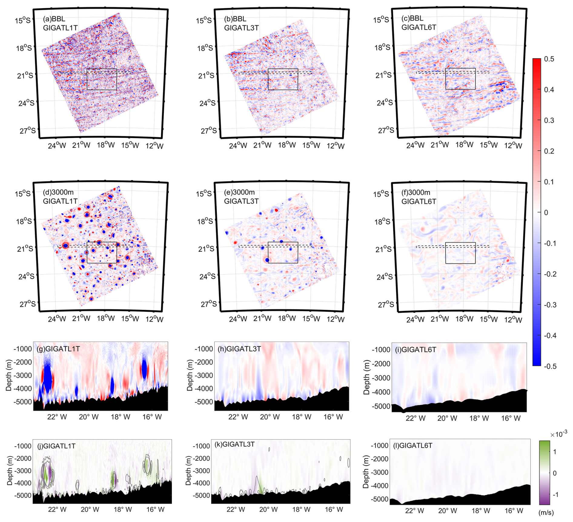
Figure 2 5 d averaged vorticity field in GIGATL1T (a, d), GIGATL3T (b, e) and GIGATL6T (c, f) at the top of the BBL (a–c) and at 3000 m (d–f); vorticity profiles along 21° S (dash square in a–f) in the GIGATL1T (g), GIGATL3T (h) and GIGATL6T (i) simulations and vertical velocity across the same transect (j–l). In (j, k), contour lines represent vertical vorticity normalized by the Coriolis parameter ($\mathit{\zeta }/f$), with specified levels at −0.5, −0.25, 0.25, and 0.5 in the GIGATL1T case (j), and at −0.25, −0.125, 0.125, and 0.25 in the GIGATL3T simulation (k).

2.1.3 Tracer Particles Tracking

To quantify the modelled mixing, we performed offline Lagrangian particle tracking simulations with Ichthyop (Barrier et al., 2026), an open-source Java-based Lagrangian model designed for particle simulations in σ-coordinate models like CROCO. Ichthyop reads the time-varying CROCO velocity fields and then advects virtual particles according to:

$$\begin{array}{}\text{(3)}& {\displaystyle \frac{\mathrm{d}\mathit{x}}{\mathrm{d}t}}=\mathit{v}(\mathit{x},t)\end{array}$$

where the vector $\mathit{x}=\mathit{x}(x,y,z)$ represents the position of the particles, and v represents the three-dimensional Eulerian velocity interpolated at the particle location at time t.

We released strictly passive particles, with no explicit diffusion or random walk component added, ensuring the diffusivity estimates reflect mixing in CROCO (both numerical and parameterized mixing). We released in each simulation five clouds of 10 000 tracer particles around the BBTRE site (all over the solid line box in Fig. 2), one every two days during 1–9 July 2009, at three depths, in the bottom-most model layer (about 40 m above the seafloor), at 3000 and at 4000 m. The initial standard deviation of the vertical spread of tracer (σ₀) was set to 9 m, as measured in the BBTRE. Each particle was tracked for 20 d.

In the 1 and 3 km simulations, where eddies are formed in large numbers through interactions of the flow with the bathymetry (Sect. 3.1), clouds of particles were also released in the annular region between 1.2 and 3 eddy radii of the surrounding coherent eddies, as well as in the background flow between eddies. Examples of the release strategy are provided in Fig. A1.

2.1.4 Estimated Diffusivity

Diapycnal (vertical) diffusivity K was diagnosed with two complementary methods: (i) K_z obtained from a tracer–moment estimate based on the density variance of the spread of tracer particles, and (ii) K_BBL obtained as a layer-mean estimate of diapycnal diffusivity within the BBL.

K_z is obtained from the spreading rate of the particles in the density field following the tracer-moment method described in Ruan and Ferrari (2021). More specifically, K_z is obtained as

$$\begin{array}{}\text{(4)}& K_z={\displaystyle \frac{\mathrm{1}}{\mathrm{2}}}{\displaystyle \frac{\mathrm{d}}{\mathrm{d}t}}\left[{\displaystyle \frac{\langle (\mathit{\rho }-\langle \mathit{\rho }\rangle {)}^{\mathrm{2}}\rangle }{\mathrm{|}\mathrm{\nabla }\mathit{\rho }{\mathrm{|}}^{\mathrm{2}}}}\right]\end{array}$$

where ρ is density, and ∇ρ is the local density gradient. This formulation relates the growth of tracer variance to diffusivity, but is generalized to stratified flows by considering tracer moments in buoyancy coordinates. To avoid biasing the estimate of vertical diffusivity by combining particles sampling different stratification regimes, the initial particle release region was partitioned into multiple three-dimensional bins in longitude, latitude, and depth. Within each bin, diapycnal diffusivity was estimated from the trajectories of particles released in that bin. The resulting estimates were then combined using particle-number weighting to obtain the domain-integrated K_z.

For a more direct comparison with the BBTRE data, in the case of the release right atop the BBL, we also considered an inverse model that removes the spatial and temporal variations from the background field following Ledwell (2024) and according to:

$$\begin{array}{}\text{(5)}& K_{\text{BBL}}={\displaystyle \frac{UH\left(\frac{\mathrm{d}{\mathit{\rho }}_{\text{BBL}}}{\mathrm{d}x}\right)}{\frac{\partial {\mathit{\rho }}_{\text{BBL}}}{\partial z}}}\end{array}$$

where U is the mean flow lateral velocity over the release region during the trajectories and H is the bottom boundary layer thickness, assumed to be constant in space, and ρ_BBL is the density at the top of the BBL.

3 Results

3.1 The simulated flow field

From an observational perspective, the near surface circulation of the Brazil Basin is characterized by a weak sub-inertial flow (i.e. eddies), while the deep waters dynamics are thought to be controlled by inertial motions induced by the interaction of the flow with the topography (Polzin, 2009). In the CROCO simulations, the upper layers confirm low levels of eddy kinetic energy compared to other areas of the Atlantic, while the modeled BBL is occupied by incoherent vorticity perturbations and numerous, but short lasting, submesoscale eddies and vorticity filaments. The absence of major mesoscale systems in the BBL agrees with the low eddy kinetic energy levels measured in the Deep Basin Experiment. The near-bottom mean currents (Fig. A2), however, have amplitudes generally slightly larger than observed values. In the BBL, the vorticity is more intense with increasing resolution, with abundant filaments and small submesoscale eddies in the 1 km cases. Above the BBL, on the other hand, many mesoscale and submesoscale eddies populate the vorticity field in the GIGATL1 and GIGATL3 simulations, and they are more abundant and intense in the GIGATL1 runs, where they are characterized by a local R_o ∼ 1 and are often surrounded by a ring of intense, opposite-signed relative vorticity (Fig. 2d–f, shown at 3000 m depth). Only a few and very weak mesoscale structures form in the GIGATL6 run. The generation of a rich deep eddy field is independent of the vertical discretization choice, and was already noted in km-resolution simulations of the same region using the MITgcm ocean model in its hydrostatic configuration, albeit in a less realistic setup (Drake et al., 2022b).

The eddies have a size close to the baroclinic Rossby radius of deformation (∼ 50 km) and extend to about 2000 m (Fig. 2g and h). Their generation in the GIGATL1 and GIGATL3 runs is independent of tidal presence (Fig. A3), and the eddies are characterized by enhanced vertical velocities at their periphery (Fig. 2j and k). On the contrary, the coherent eddies are largely absent in GIGATL6T and the vertical velocities do not display significant patterns (Fig. 2l).

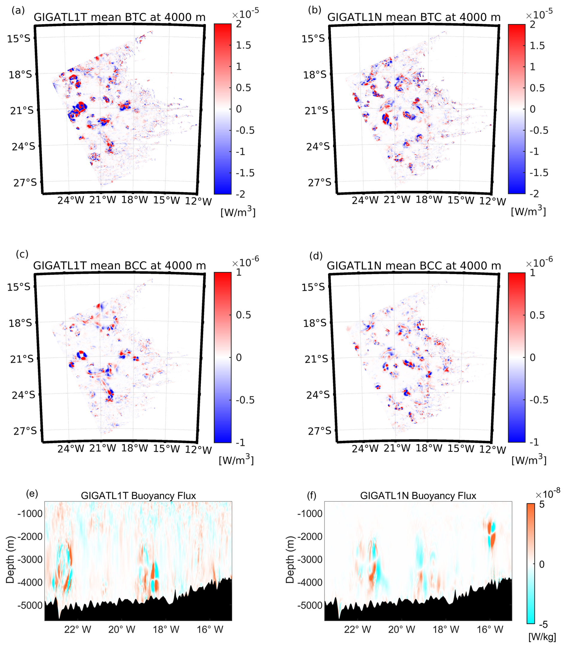
Figure 3 Monthly mean of BTC (W m⁻³) (a–b) and BCC (W m⁻³) (c–d) at the depth of 4000 m in GIGATL1T and GIGATL1N. Profiles of 5 d averaged buoyancy flux along 21^oS in (e) GIGATL1T and (f) GIGATL1N.

The marked difference in eddy coherence in and above the BBL (Fig. 2) suggests differing energy cascade dynamics near the bottom versus the interior ocean. Bottom interactions prevent the formation of mesoscale structures, while in the interior such formation is promoted. Both barotropic and baroclinic processes are at play according to the energy conversion analysis (Fig. 3a–d). BTC (barotropic conversion) is consistently about one order of magnitude larger than BCC (baroclinic conversion) in the deep water column.

The formation of mesoscale eddies locally enhances the EKE of the flow via buoyancy fluxes and consequently mixing, as suggested by $\stackrel{\mathrm{‾}}{{\mathit{\omega }}^{\prime }{b}^{\prime }}$ shown in Fig. 3e and f. ω^′ and b^′ are the vertical velocity and buoyancy perturbations to the monthly-averaged background flow (Gula et al., 2022). Enhanced vertical covariance can be found inside and around the eddies in the GIGATL1 simulations, independently of the tidal presence, while it is much weaker in the GIGATL3 runs (Fig. A4) where the eddies are less intense, and nearly absent in the 6 km run (Fig. A4). In the background flow between the eddies, on the other hand, only the tidal presence supports buoyancy exchanges (Figs. 3 and A4).

3.2 Lagrangian Tracer Particles Release Experiment

Next, we quantify how the differences in the flow field (stronger/weaker eddies and presence/absence of tidal-induced buoyancy exchanges) translate into different representations of vertical transport and mixing across the five simulations.

The particle vertical displacement in density space and dispersion A², quantified as $A^{\mathrm{2}}(t;t_{\mathrm{0}})=\frac{\mathrm{1}}{N}{\sum }_{i=\mathrm{1}}^N\mathrm{|}z\left(t\right)-z\left(t_{\mathrm{0}}\right){\mathrm{|}}^{\mathrm{2}}$, where N represents the total number of particles released in the targeted region, z(t) denotes the position of the ith particle at time t, and t₀ is the initial release time, are shown in Fig. A5.

In the BBL, the vertical dispersion follows a ballistic regime for about one day, then the curves display slopes ranging from A² ∼ t^0.75 to A²∼t¹. In this regime (day 2 to day 20), the vertical dispersion is greater in the GIGATL1 runs than in the GIGATL3 and GIGATL6 simulations (Fig. A5), as found in analogous comparisons at the ocean surface (Zhong and Bracco, 2013). Tidal motions play a lesser role compared to model resolution, with the vertical dispersion in the tidal integrations slightly exceeding that of the no-tide cases in the GIGATL3 runs and being nearly indistinguishable after the first day in the GIGATL1 simulations, especially at the bottom layer. Higher in the water column, at 3000 m, the slopes of the dispersion curves are around 0.5–0.7 in the tidal runs, suggesting that eddies may modulate vertical dispersion (Callies, 2018; Drake et al., 2022a; Yankovsky et al., 2022). In the water column, the presence of tides has a greater impact than in the BBL.

In terms of displacement, particles in the GIGATL1 runs form thin filaments while maintaining an approximately Gaussian overall distribution, and they spread more thoroughly than in GIGATL3 and GIGATL6. Displacement is also slightly greater when tides are included. The inclusion of tides intensifies vertical velocities and increases vertical displacement, but the enhancement in tidal simulations remains secondary to the resolution effect. The enhancement is greater in the GIGATL3 case than in the GIGATL1 simulations.

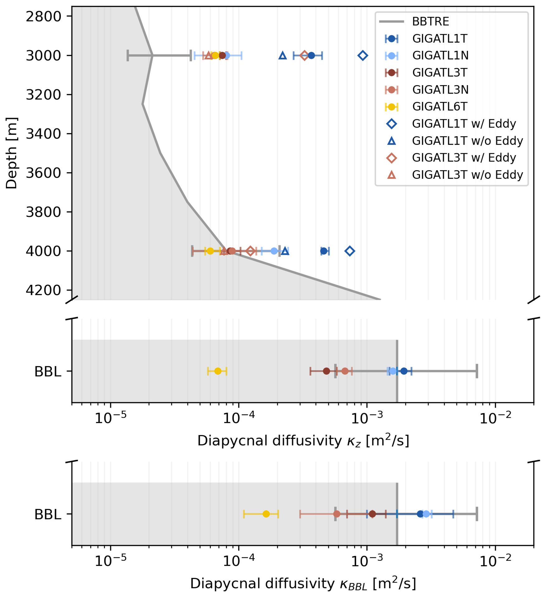
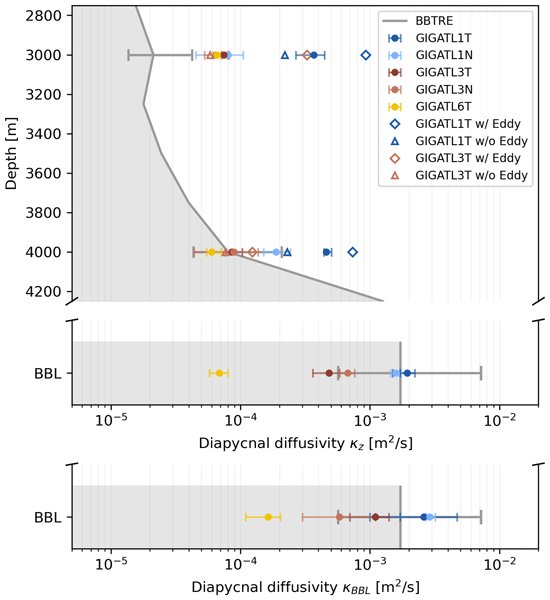
Figure 4 Diffusivities in the abyssal Brazil Basin in the observations and the five GIGATL simulations: vertical diapycnal diffusivity K_z, and BBL diffusivity K_BBL. Gray shading and lines represent BBTRE observations. Horizontal bars indicate ranges (max-min) across sampled patches and the depths at which tracer particles were released in the CROCO simulations. Values from releases around eddies or in the background flow at 3000 and 4000 m depth are also indicated.

3.3 Estimated Diffusivity

Next, we diagnose the vertical diapycnal diffusivity, and compare it to the values obtained from the BBTRE.

The vertical structure of K_z in GIGATL1, GIGATL3 and GIGATL6 is shown in Fig. 4. The modeled diapycnal diffusivity is enhanced toward the bottom and decreases moving away from it, which is consistent with the BBTRE measurements. Independently of the definitions used, diffusivity is higher in the GIGATL1 runs than in the lower resolution cases. As anticipated by the energetic analysis, K_z increases with horizontal resolution, and tidal motions impact K_z in GIGATL1 more so than in GIGATL3 at all depths.

Comparing our modeled diapycnal diffusivity with observational estimates in the Brazil Basin is complicated by the different vertical resolution of the model compared to the in-situ measurements, and by differences in spatial coverage between observed dye and modeled tracers. Nonetheless, the GIGATL1 simulations compare well to published observed values atop the BBL. Field measurements in BBTRE showed diffusivities of 2–4 × 10⁻⁴ m² s⁻¹ at about 500 m above an abyssal hill (Ledwell et al., 2000), increasing to over 10⁻³ m² s⁻¹ in the BBL, and the GIGATL1 simulations show very good agreement, with a slight underestimation for GIGATL3 and a substantial one for GIGATL6. Above the BBL, at 4000 m depth, however, only the GIGATL6, GIGATL3 and GIGATL1N diffusivities are within the observed values considering uncertainties, while the diffusivity in GIGATL1T overestimates the observations. Higher up in the water column, the modeled diffusivities overestimate the observational values in all runs, with a larger bias in the GIGATL1T case. In GIGATL6, the diagnosed diapycnal diffusivity is lower than in the 3 and 1 km simulations and nearly constant (6–$\mathrm{8}\times {\mathrm{10}}^{-\mathrm{5}}$ m² s⁻¹) throughout the water column. Overall, mixing does not decline with height in any of the simulations as sharply as it does in the observations.

The energy conversions and vertical dispersion analysis point to eddies as key players in modulating the modeled diapycnal diffusivity, with tides contributing only to the diffusivity of the background field. To further quantify the contribution of the eddies to the interior diffusivity, we conducted several sensitivity experiments by altering the tracer release locations in GIGATL1 and GIGATL3. GIGATL6 was excluded in this case due to the absence of coherent structures. Narrowing the tracer release to only eddies or background areas, including a release at the exact location of BBTRE (21.7° S, 18.3° W) changes our modeled estimates. Whenever the tracers are placed in the background around the coherent eddies, they undergo a smaller amount of diapycnal mixing. Vice versa, mixing is enhanced (about 2–4 times as much as in the background in the GIGATL3 case and more than three times larger in the GIGATL1 simulations) in and especially around the eddy cores.

Last, we compare our K estimates with prior modeling studies. Using the MITgcm configured in a semi-idealized domain resembling the BBTRE release location at 600 m horizontal resolution, Drake et al. (2022b) estimated K_z near the bottom using Eq. (4) modified to account only for temperature. They found a diffusivity value of about 1.50 × 10⁻³ m² s⁻¹ at day 25 from the release of the tracers, which is broadly consistent with our GIGATL1 values. Moving to other regions, Mashayek et al. (2024) investigated the enhancement in BBL turbulence induced by shear and submesoscale instabilities in seamount wakes. They focused on the New England Seamounts in the North Atlantic and estimated the diapycnal diffusivity to exceed 1 × 10⁻³ m² s⁻¹ within a few hundred meters over the seafloor, especially around wake vortices as a result of an active submesoscale field. Similar values were captured by submesoscale-permitting simulations of the Gulf of Mexico (Bracco et al., 2016), and in agreement with tracer release observations at the same location (Ledwell et al., 2016).

4 The realism of the modeled world: Bathymetric smoothing and the modeled eddy field

In the simulations, diapycnal mixing is modulated by the eddy field, with tides having a secondary role and not impacting the evolution of the eddy field whenever the Rossby deformation radius of the BBL is resolved (Figs. 2 and A3). However, both theory (e.g., Munk and Wunsch, 1998) and observations (e.g., Polzin et al., 1997; Ledwell et al., 2000) identify internal waves generated by tide–topography interactions as an important driver of diapycnal mixing in the deep ocean in regions of steep topography. When the internal wave trajectories parallel the topographic slope, linear wave theory predicts that wave propagation would be limited, waves would break and, through this process, mixing in the BBL would be enhanced (Polzin and McDougall, 2022; Buijsman et al., 2026). The reason for such fundamental differences between theoretical predictions, observations and model outcomes can be understood considering how model resolution and bathymetric smoothing, which is required by models due to their discretization, affect the partition of energy among the mean flow, eddies, and internal waves.

The GIGATL6 is too coarse to represent the interactions between the steep bathymetry and the flow. As a result, eddies are very few and weak, and the internal wave field is strongly underestimated, with diapycnal mixing approximately constant across the water column, mostly controlled by the numerics.

Although the GIGATL1 and GIGATL3 simulations are at a resolution high enough to permit mesoscale and in part submesoscale dynamics, and they provide a reasonable representation of the small-scale topographic variability – GIGATL1 more so than GIGATL3 –, the topography remains too smooth to efficiently block and contract scattered internal tides, generating an intense eddy field instead.

We assess the consequences of this smoothing by considering the moments of the topographic height spectrum H(k) for GIGATL1, GIGATL3 and GIGATL6 and multibeam observations. The nth moment can be represented as

$$\begin{array}{}\text{(6)}& \underset{\mathrm{0}}{\overset{\mathrm{\infty }}{\int }}{k}^{n}H\left(k\right)\mathrm{d}k\end{array}$$

For abyssal hills, H(k) is commonly fractal, i.e. for high horizontal wavenumbers k, $H\left(k\right)\propto k^{-x}$ with $\mathrm{2}<x<\mathrm{3}$, see also Fig. 5.

Table 1 Moments of the topographic spectrum H(k), Eqs. (6) and (7). We find that the second moment is of similar magnitude as the square of the semi-diurnal ray trajectory slope, with N = 1 × 10⁻³ s⁻¹. See Polzin (2004, 2009) for further discussion of the dimensions and O(1) pre-factors.

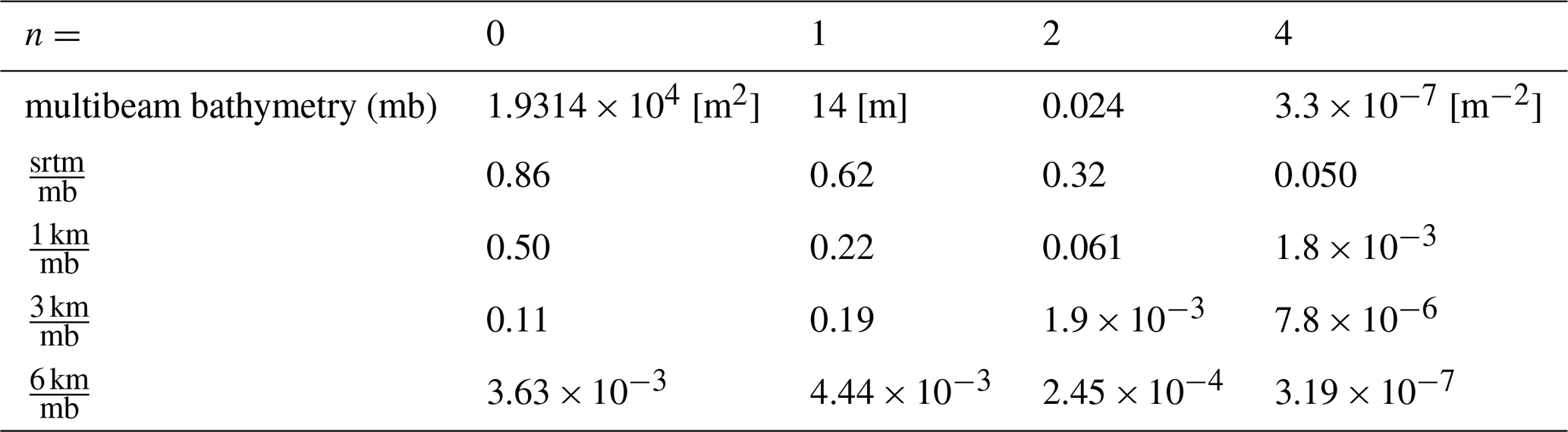
Table 1 compares the moments associated with four data sets of the Brazil Basin bathymetry using a normalized spectral moment truncated at k_cut:

$$\begin{array}{}\text{(7)}& {\displaystyle \frac{{\int }_{\mathrm{0}}^{k_{\text{cut}}}{k}^n{H}_{\text{mb}}\left(k\right)\mathrm{d}k}{{\int }_{\mathrm{0}}^{k_{\text{cut}}}{k}^n{H}_{\mathrm{\dots }}\left(k\right)\mathrm{d}k}}\end{array}$$

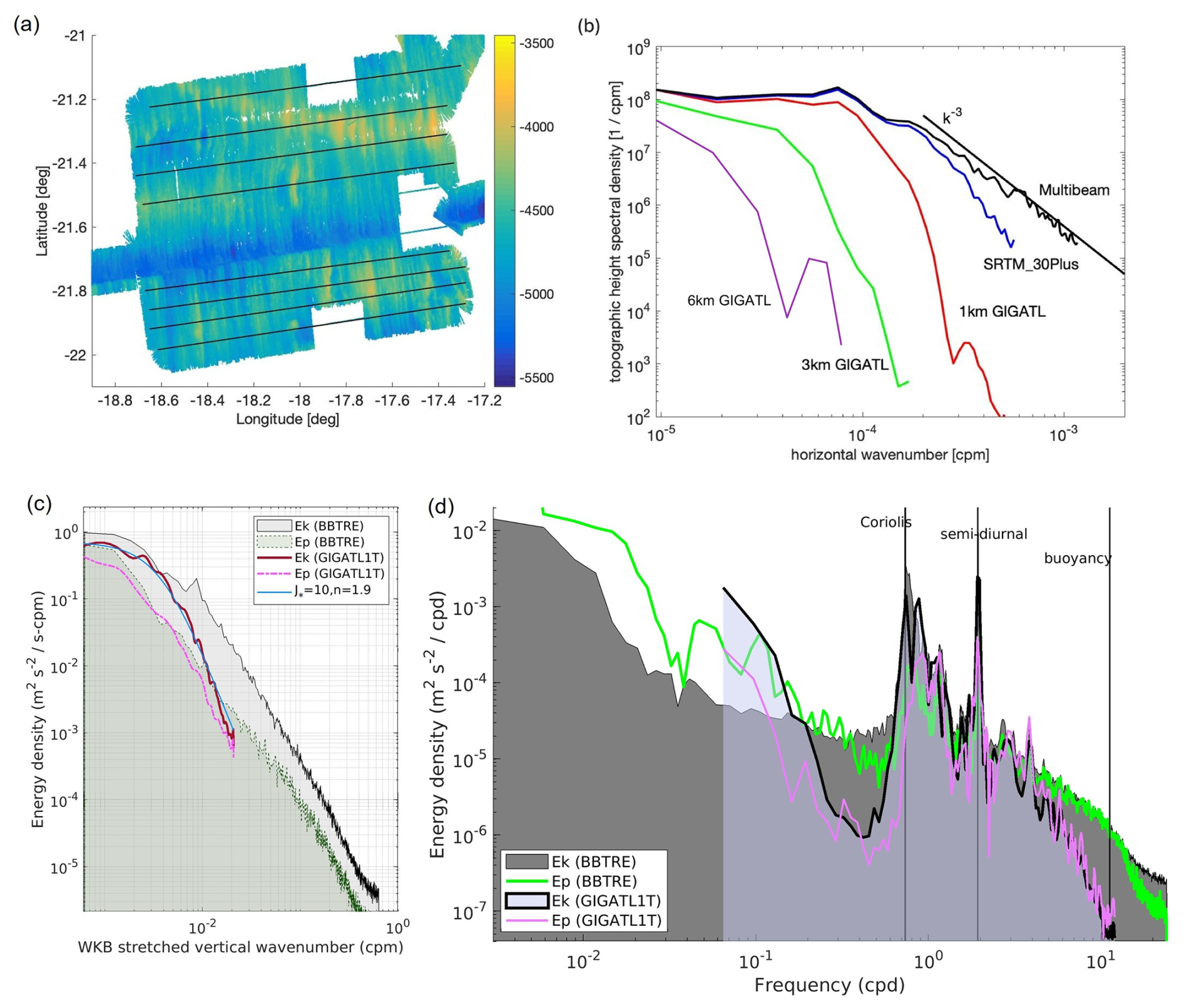
Figure 5 (a) multi-beam topography from the vicinity of the BBTRE tracer injection site. Ping data were mapped onto a 50 m grid and this map was used to create estimates of bathymetry vs distance along the indicated lines. (b) Estimates of bathymetry from the SRTM_30plus data set and the GIGATL grids were interpolated onto the multi-beam product coordinates. All datasets were Fourier transformed to quantify the impact of filtering in the four derivative representations. (c) Stretched vertical wavenumber spectra using Wentzel-Kramers-Brillouin (WKB) approximation of horizontal kinetic (Ek) and potential energy (Ep) using BBTRE data and the GIGATL1T run. The blue line represents a fit of the GM (Garrett–Munk) model: $(j_{\ast }^{\mathrm{2}}+j^{\mathrm{2}}{)}^{-n}$, which provides an estimate of the background internal-wave energy under approximate horizontal isotropy and scaling with local stratification, while j represents the vertical wavenumber with the scale height of 1300 m. (d) Horizontal kinetic energy and potential energy frequency spectra at BBTRE site at 3000 m for the observations and the GIGATL1T simulation.

We considered multibeam data from nearby the tracer injection site in the Brazil Basin shown in Fig. 5a and the topographic height spectral density H_mb(k) shown in Fig. 5b, the SRTM_30 plus product H_srtm(k), the GIGATL1 bathymetry H_1 km(k), the GIGATL3 bathymetry H_3 km(k) and GIGATL6 bathymetry H_6 km(k). The implication of our analysis is that the integral for the first moment converges, but not the second, or fourth. Linear wave kinematics prescribes a rate of energy transfer from the barotropic to baroclinic tide (generation) proportional to the first moment, while the energy density of the internal tide is proportional to the second moment and the shear variance, which relates to wave-breaking, is proportional to the fourth moment. Finescale parameterizations then connect turbulent dissipation to the square of this fourth moment. A prediction of infinite second moment implies infinite energy density, which is of course unfounded, and theoretically is avoided by using a quasi-linear model of wave generation which places the linear analysis in the advected coordinate of the barotropic tide. This effectively regularizes the integrals defining the moments (Eq. 6) by introducing an integration endpoint of approximately $k_{\text{cut}}=\mathrm{1}/{\mathit{\lambda }}_{\mathrm{h}}=\mathit{\sigma }/\mathrm{4}{U}_{\mathrm{0}}$, where k_cut is set to be equal to the Nyquist wavenumber of the SRTM and model products. U₀ represents the velocity amplitude of the barotropic tide and σ its frequency. λ_h is about 1 km in the Brazil Basin, significantly smaller than the 6–8 km distance between hill crests, and a velocity amplitude of U₀ = 0.03 m s⁻¹ maps well onto a peak in the observed near-bottom vertical wavenumber shear spectrum.

The results summarized in Table 1 imply an energy transfer from barotropic to baroclinic tides. Even in the higher resolution GIGATL1 case, there is nearly an order of magnitude difference in the second moment (energetics) and an even greater underestimation for the model fourth moment (shear variance). Our interpretation is that the smoothing of the bathymetry in the GIGATL runs, and more generally in ocean models, alters both the generation of the eddy field and the pathways through which its energy can be transferred toward smaller scales. Smoothed topography generates reliefs that retain the key features at scales larger than 3–4 km but removes small-scale roughness, allowing isopycnal spreading over the ridge and an appreciable velocity curvature U_zz. The resulting flow facilitates baroclinic and submesoscale instabilities which convert available potential energy into eddy kinetic energy, supporting the generation of strong eddies. Rough topography in the real ocean, on the other hand, provides an important pathway through which geostrophic and tidal motions can transfer energy into the internal-wave field, ultimately feeding small-scale shear and turbulent dissipation (Polzin, 2004, 2009; Nikurashin and Ferrari, 2010). With a smoothed topography, CROCO generates less of these waves than the real ocean, the eddy field loses a principal energy sink and the result is a more energetic flow field. Eddies persist at higher amplitude and contribute to an elevated diffusivity that extends to the ocean interior, and to an overall barotropization of the water column, as found near the surface as well (Yankovsky et al., 2022). Bathymetric smoothing therefore has the potential to affect both sides of the eddy–internal-wave energy partition.

To confirm our interpretation of the results and further quantify the role of bathymetric representation, we performed an additional sensitivity experiment using the bathymetry of the GIGATL3T run in a regional simulation at the resolution of 1 km. This experiment develops substantially fewer coherent deep eddies and weaker relative vorticity than GIGATL1T (Fig. A6), and the resulting circulation more closely resembles GIGATL3T. Thus, increasing horizontal resolution alone is not sufficient to reproduce the energetic eddy field found in GIGATL1T. Together with the consistency with geostrophic mean circulation among GIGATL1, GIGATL3, and GIGATL6, the sensitivity experiment points to the representation of the underlying topography as a primary control on the differences in the simulated eddy field.

Table 2 Eddy deformation and diagnosed horizontal energy conversion to the internal-wave field in GIGATL1T, GIGATL3T, GIGATL6T and in the sensitivity run, averaged over 3000–5000 m in the subregion (20–22° S, 17–20° W)

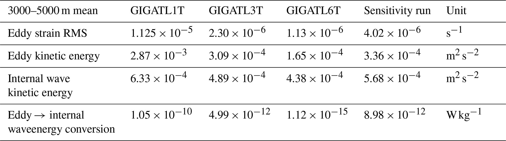
The energy exchange diagnostics introduced in Polzin (2010) further illustrate how the generation of an intense eddy field modifies the abyssal energy partition. Following Polzin (2010), we diagnose the horizontal exchange between the eddy and internal-wave fields from the covariance between internal-wave stresses and eddy strain (Table 2). Averaged between 3000 and 5000 m, eddy kinetic energy in GIGATL1T is approximately nine times that in GIGATL3T, while the RMS eddy strain is nearly five times larger. The diagnosed eddy-to-internal-wave energy conversion also increases strongly, by approximately a factor of 21. However, the resolved internal-wave kinetic energy increases by only about 30 %. Thus, the higher-resolution bathymetry in GIGATL1 facilitates stronger coupling between the eddy and internal-wave fields, while the resulting increase in the resolved internal-wave reservoir remains far smaller than the increase in eddy energy. This is consistent with the 1 km bathymetry still being too smooth to support internal-wave generation and scattering sufficient to act as an effective sink of energy.

The sensitivity run confirms that at the first order bathymetrical detail, and not resolution per se, controls the energy conversion.

The key differences in bottom roughness between model and observations can be further assessed considering the differences in the vertical wavenumber spectra. The vertical wavenumber spectrum and horizontal KE spectra for the deep Brazil Basin in the GIGATL1 runs and in the observations are compared in Fig. 5c and d. The model captures the observed near-inertial peak. In horizontal wavenumber space, the modeled and observed spectra agree reasonably well at low wavenumbers, yet the energy in CROCO decays too fast at high wavenumbers. The model vertical wavenumber bandwidth (i.e. j_∗) is also slightly smaller than the observations, speaking to the impacts of CROCO finite spatial resolution, which, in combination with the smoothed topography, acts on the representation of the generation and scattering processes. The more rapid spectral roll-off compared to observations suggests an inefficient forward cascade of energy to fine scales in the simulation. Indeed, the model retains much of its energy in long-lived, coherent mesoscale eddies.

The vertical wavenumber spectra for both the model and the observational data document relatively low KE to PE ratios at the largest resolved vertical wavelengths, increasing at 500 m wavelength. We interpret such increasing ratios as a result of parametric subharmonic instability transfers from the semi-diurnal internal tide to near-inertial waves. The model near-inertial field, however, is less developed than in the observations. At subinertial frequencies, the model spectra indicate decidedly greater eddy variability at periods of 10 d, which we attribute to the submesoscale field. The field record extends to nearly two years and documents the presence of longer periods that we cannot presently assess.

Again, this analysis supports the hypothesis that the smoothed model bathymetry limits the transfer of energy toward the high-wavenumber internal-wave field. Although the higher-resolution GIGATL1 bathymetry permits stronger eddy-internal-wave coupling than GIGATL3, the model still lacks the finescale internal-wave energy observed over the rough Brazil Basin topography. The resulting internal-wave pathway therefore remains an insufficient sink for the energy with the generation of an energetic eddy reservoir instead. The coherent eddies, in turn, contribute to elevated diffusivity in the ocean interior.

5 Conclusions

The genesis of enhanced turbulent mixing above rough topography has been discussed extensively in recent decades (Polzin and McDougall, 2022). Given the role that diapycnal mixing plays in shaping the distribution of heat and carbon and the overall overturning circulation, it is paramount to capture its variability in time and space. Observations remain limited and model simulations are strongly constrained by resolution, vertical discretization choices, approximations adopted – most commonly the hydrostatic assumption – and parameterization schemes implemented, or, in the case of direct numerical simulations, size and realism of the integration domains. The contribution of each dynamical process involved with diapycnal mixing in the BBL remains unconstrained, especially in regions characterized by very rough topography. This is the case of the Brazil Basin, where topographic features are of order O(1) km.

Diapycnal mixing in the deep Brazil Basin is known to be significantly elevated over rough bathymetry and decline when moving into the ocean interior (Polzin et al., 1997). The GIGATL simulations at 1 and 3 km horizontal resolution, with and without tide, reproduce this trend: K peaks near the bottom and declines with height, and in the BBL is broadly consistent in magnitude with that observed during the BBTRE campaign. If eddies do not form (GIGATL6 runs) then K is approximately constant in the water column and controlled by the numerics (parameterization and parameterization coefficients). However, at 1 km horizontal resolution modeled diffusivities are overestimated in the ocean interior. This discrepancy suggests that CROCO fails to suppress excessive mixing in the stratified interior, and mesoscale eddies emerge as critical in the abyssal Brazil Basin. The instabilities that occur over rough topography as represented by the model facilitate the generation of eddies that extend from the BBL into the water column, displacing isopycnals. Localized increased vertical mixing is found around and within these eddies, which are stronger and more numerous in the GIGATL1 simulations because the scale of the instabilities responsible for their generation is better resolved. At the resolutions considered in this work, the enhanced eddy reservoir can outpace the model's ability to transfer energy toward the internal-wave and ultimately dissipative pathways, contributing to overestimated diffusivities in the ocean interior. At the same time, the model underestimates the high-wavenumber energy because the smoothed topography precludes a realistic internal wave generation. In summary, two non-exclusive processes explain the eddy–wave partitioning in the model simulations: on one hand, buoyancy anomalies favorable to baroclinic instability are amplified relative to reality; on the other, the absence of a realistic internal-wave field removes an energy sink that would otherwise damp the eddy field.

As note of caution, we stress that beyond eddy dynamics, vertical mixing parameterizations and the numerical schemes employed also contribute to the biased interior diffusivity. The GIGATL runs employ the k−ε parameterization. Compared to the widely used KPP (Large et al., 1994) parameterization, the k−ε is more sensitive to background settings and to the imposed vertical–mixing value (Warner et al., 2005), which in our runs attains a minimum value of turbulence kinetic energy (TKE) (tke_min = 10⁻⁶).

Also, the numerically induced contributions to mixing relevant to the terrain-following coordinates need to be considered. Schifano et al. (2025) showed in CROCO that numerical diapycnal mixing can become substantial over steep slopes, even when rotated tracer-advection schemes are used, because the rotation of the diffusive operator is constrained by the grid geometry. Their results also highlight that additional topographic smoothing reduces numerical mixing, but simultaneously removes small-scale bathymetric structure that is dynamically important for flow–topography interactions.

In closing, the comparisons among the five simulations considered and the observations highlight that in mesoscale-resolving/submesoscale-permitting ocean models, horizontal resolution modulates vertical diapycnal diffusivity and mixing more than tidal forcing. Even at 1 km, the smoothing applied to the bathymetry removes high-wavenumber roughness. As a result, the high-mode internal-tide shear and the consequent wave-breaking contributions are underestimated, causing the energy to remain concentrated inside the eddies, which are likely more numerous and intense in the model runs than in the real ocean. The outcome is that over rough topography increasing model resolution to a submesoscale-permitting regime may produce unrealistic, overestimated diffusivities in the ocean interior, and, counterintuitively, more so than in simulations that cannot resolve the submesoscale instabilities responsible for the eddy generation.

In summary, in the case of ocean diapycnal mixing, resolution alone is not the answer, and further research is needed to improve the realism of traditional ocean models and of the emerging machine learning based ocean emulators, often trained on submesoscale-permitting runs. Furthermore, nonhydrostatic model simulations are needed at finer horizontal and vertical resolution, which would be valuable for future process studies to advance our understanding of the interactions between internal waves, rough topography, submesoscale instabilities and their impact on the diapycnal mixing and buoyancy transformations in and above the BBL. Moving forward, observational constraints are required to establish how often and by how much the relative contributions of the eddy versus internal wave fields in the BBL are misrepresented in state-of-the-art ocean models. These constraints would also allow us to better validate the residence time of heat and carbon across the water column.

Appendix A: Additional Figures

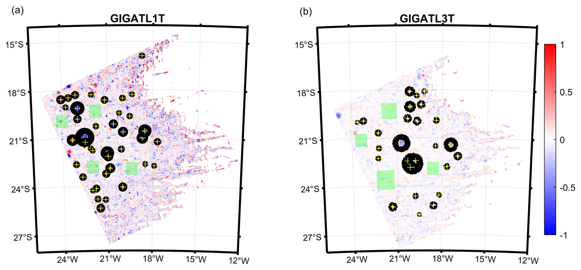
Figure A1 Particle release locations in the GIGATL1T (a) and GIGATL3T (b) simulations at 4000 m depth. Relative vorticity is shown in color in the background. Yellow crosses mark the centers of detected eddies. Black circular regions indicate particle releases surrounding coherent eddies, while green boxes indicate releases in background-flow regions without detected eddies.

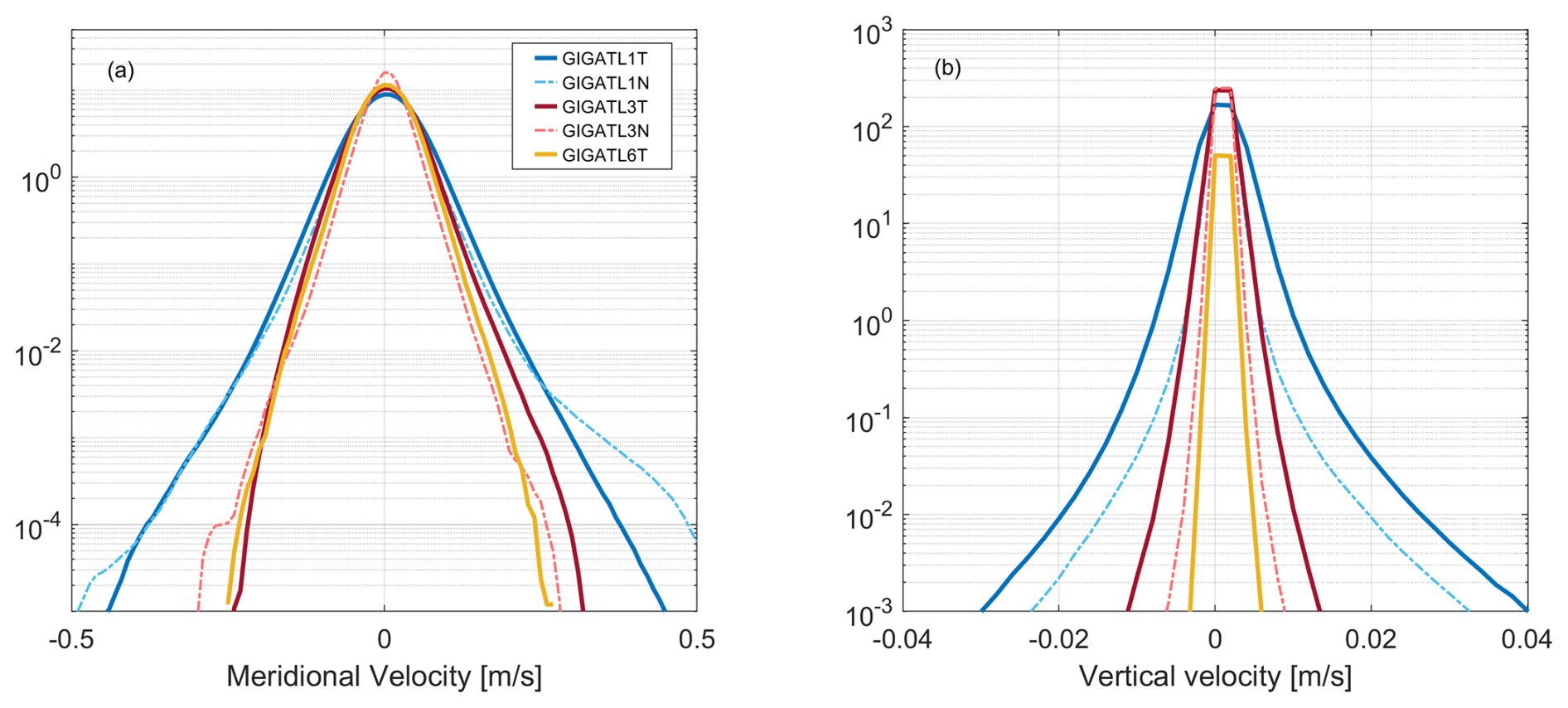
Figure A2 The probability density functions of (a) meridional velocity in m s⁻¹, (b) vertical velocity at the top of the BBL in m s⁻¹.

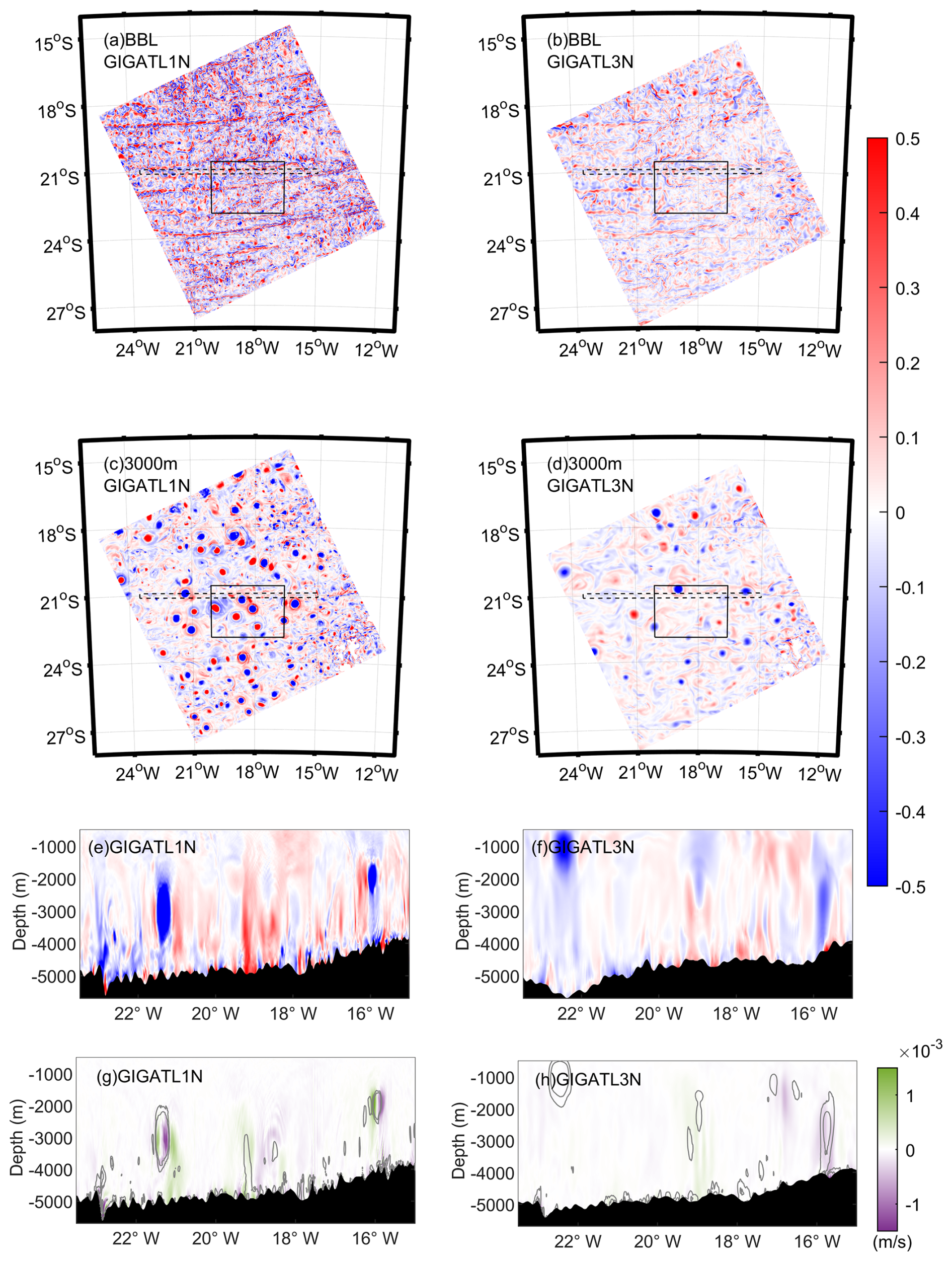
Figure A3 A 5 d averaged vorticity field of GIGATL1N (a, c), GIGATL3N (b, d) at 3000 m and at the top of BBL; vorticity profiles along 21° S (dash square in a–d) in the GIGATL1N (e) and GIGATL3N (f) simulations and corresponding vertical velocity slices (g, h). Contour lines represent vertical vorticity normalized by the Coriolis parameter ($\mathit{\zeta }/f$), with specified levels at −0.5, −0.25, 0.25, and 0.5 in the GIGATL1N cases (g), and at −0.25, −0.125, 0.125, and 0.25 in the GIGATL3N simulations (h).

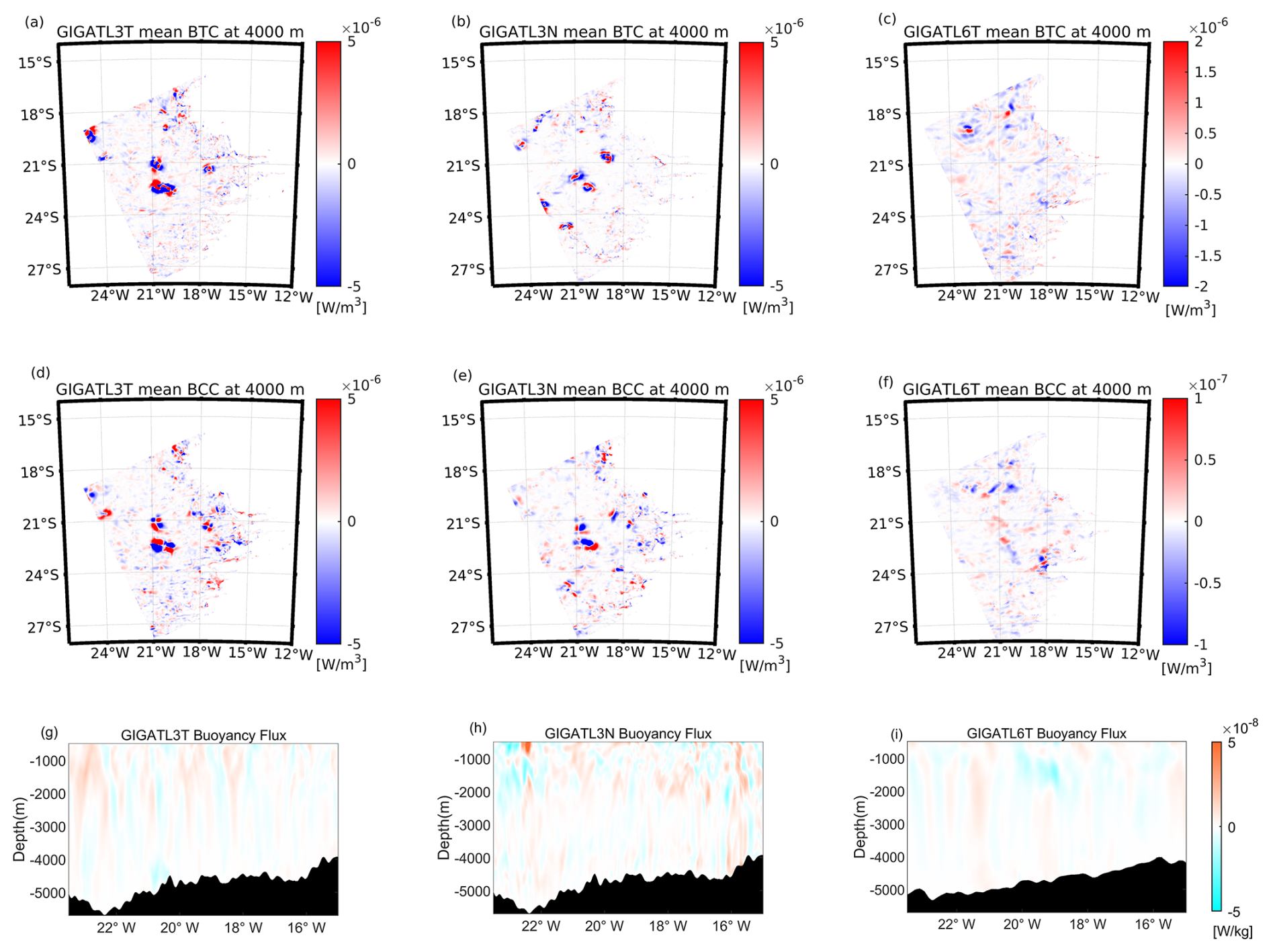
Figure A4 Monthly mean of BTC (a–c) and BCC (d–f) at the depth of 4000 m in GIGATL3T, GIGATL3N and GIGATL6T. Profiles (g–i) of 5 d averaged buoyancy flux along 21° S.

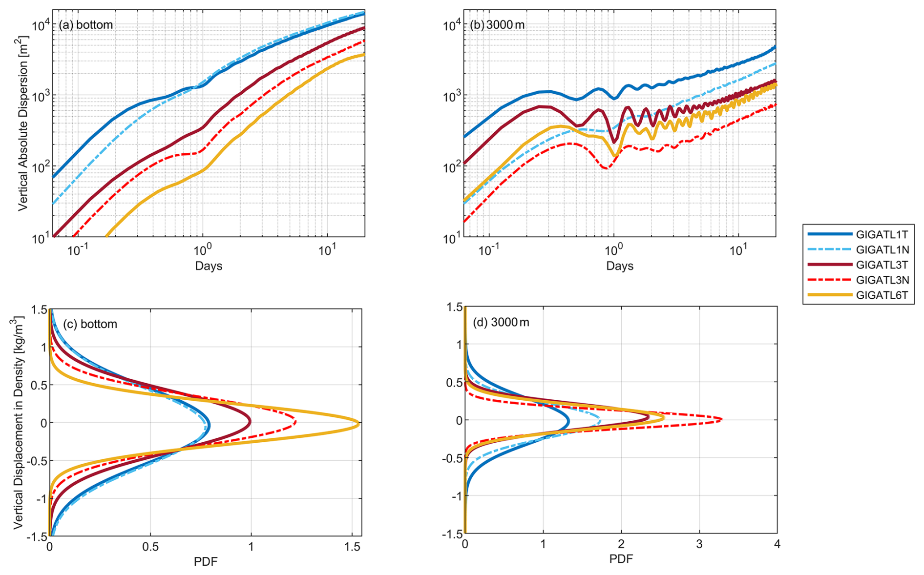
Figure A5 Vertical absolute dispersion (m²) (a, b); Vertical diapycnal displacement of tracer particles at Day 20 after release (c, d).

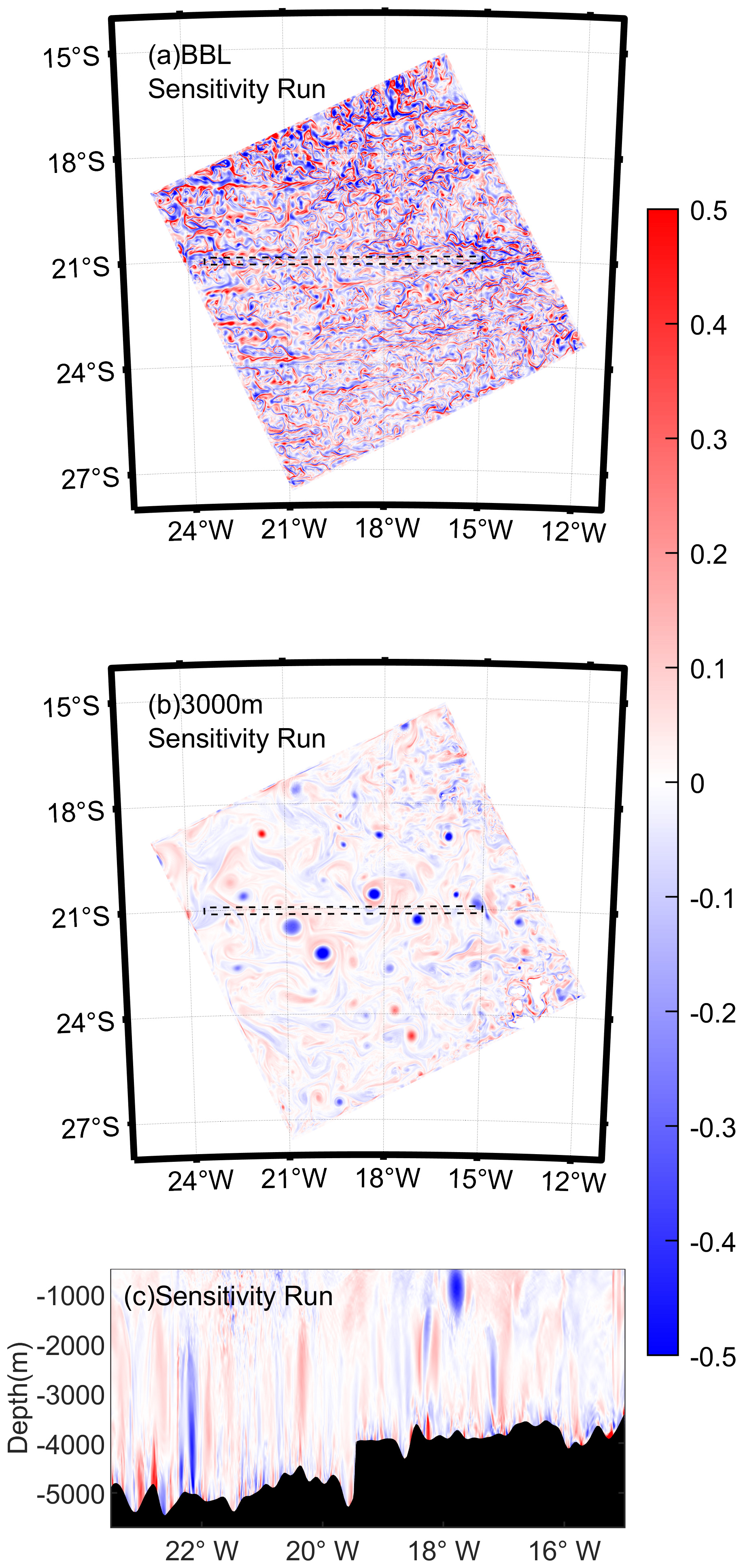
Figure A6 A 5 d averaged vorticity field of the sensitivity run at 3000 m and at the top of BBL; vorticity profiles along 21° S (dash square in a and b).