Seasonal cycle in surface seawater isotopic composition

Data of seawater stable isotopologs in the quality-controlled database from the isotopic platform facility at LOCEAN (hereafter “CISE-LOCEAN”) provide an unprecedented sampling of the surface Atlantic Ocean and the southwest Indian Ocean. This investigation of δ¹⁸O, δ²H and deuterium excess (d-excess) in surface sea water for 20 subregions indicates a large variability of the regional regression lines with salinity for δ¹⁸O and δ²H. Weakest slopes are found near the equator, and increase towards higher latitudes, but also to a lesser extent in the western Atlantic compared with the eastern Atlantic in the tropics and subtropics. These regressions often explain a large share of the variability in the data (40 % to 70 %), except for d-excess at high latitudes and δ¹⁸O, δ²H near the equator. The data are sufficient to extract a rather small seasonal variability in these relationships and an average seasonal cycle in some regions of the North Atlantic subpolar gyre, with signals probably related to changes in the input of sea ice melt and depleted water of Arctic origin. A significant correlation between observed seasonal cycles in δ¹⁸O, δ²H, and d-excess and that of salinity is found in the central equatorial Atlantic. These seasonal cycles change between the vicinity of the equator and the region to its north, which is associated with the seasonal shift of the Inter-tropical Convergence Zone and with the seasonality of the equatorial upwelling. Elsewhere, the seasonal signal usually does not emerge from the noise. An independent over 7-years long time series of nearly monthly surface sampling at the BATS site near Bermuda (31°50^′ N, 64°10^′ W) also indicates a rather well-defined seasonal cycle of surface salinity, δ¹⁸O, δ²H and d-excess. Its interannual variability in δ¹⁸O does not appear closely related to the one in salinity.

1 Introduction

Seawater isotopic composition (¹⁸O $/$ ¹⁶O and ²H $/$ ¹H ratios expressed as δ¹⁸O and δ²H in ‰ (per mille) in the VSMOW/SLAP scale) is classified as an Essential Ocean/Climate Variable (EOV/ECV) in international programs such as GEOTRACES and GO-SHIP, respectively aiming to improve the understanding of biogeochemical cycles, and to develop a globally coordinated network of sustained hydrographic sections as part of the global ocean/climate observing system. Except for fractionation during phase changes, thus mostly at the sea surface, and meteoric inputs from the atmosphere and the land masses, the water isotopic composition is nearly conservative in the ocean, with chemical and biological processes having minimal effect.

Stable seawater isotopes are used, in addition to salinity, to trace sources of freshwater (precipitation, evaporation, runoff, melting glaciers, sea ice formation and melting), as well as to characterize water masses, both at the ocean surface and in the ocean interior (Schmidt et al., 2007; Hilaire-Marcel et al., 2021). More regionally, in addition to salinity, they are used to characterize water masses and their mixing pathway into the ocean (Frew et al., 2000; Voelker et al, 2015). At the sea surface, isotopic properties of the evaporation (Benetti et al., 2014) and of regional precipitation can be used to better characterize air-sea freshwater fluxes from the surface distribution of water isotopes (Benetti et al., 2017a; Benway and Mix, 2004; Conroy et al., 2014).

There has been considerable interest in monitoring the water isotopes of sea water both at high and low latitudes. In the high latitude oceans, the formation or melt of sea ice, freshwater inputs from high-latitude rivers, and continental ice melt from marine terminating glaciers and icebergs leave strong imprints on the surface ocean isotopic composition, and for the Southern Ocean in the top 800 m water column close to ice shelves (Aoki et al., 2023; Hennig et al., 2024). These processes, as well as changes in ocean circulation vary on seasonal time scales, as well as on longer time scales up to interdecadal, which can influence the relationship between salinity and the water isotopes. At low latitudes, the surface water masses get their isotopic characteristics from ocean circulation, with in particular upwelling of water originating from subtropical evaporation-dominated regions, as well as from local evaporation, rainfall (Benway and Mix, 2004), and from the freshwater inflow of large tropical rivers, such as the Amazon River in the Atlantic Ocean (Benetti et al., 2017a). The low latitude Pacific Ocean also presents a large variability in these processes which shape the relationship between salinity and water isotopes, in particular on seasonal and interannual (such as El Niño–Southern Oscillation – ENSO) to decadal modes of variability in the southwest equatorial Pacific (Horikawa et al., 2023), the central equatorial Pacific (Conroy et al., 2017), and the South Pacific Convergence Zone (Dassié et al., 2018). Even rainfall isotopic values might change interannually, depending on the origin of the rain water, such as illustrated in the central-western Pacific in Conroy et al. (2014) or in the eastern Pacific north of the equator in Benway and Mix (2004).

These isotopic signatures in ocean water are archived in past climate records, for example, in the δ¹⁸O of carbonates from warm water corals, giant clams or planktonic foraminifera (Mulitza et al., 2003; Abram et al., 2020; Dissard et al., 2021; Dong et al., 2025), or in the δ²H of lipids (Schefuß et al., 2005; Schouten et al., 2006; Leduc et al., 2013). They are acquired from the seawater isotopic properties at the time when these organisms grow, following temperature-dependent fractionation laws. Measurements of seawater isotopes in the upper ocean is strongly recommended, often at the seasonal resolution, to understand these archives, as well as to gain a better understanding on how temperature and water isotopic properties influence the archived records, such as investigated in the recent past by Thompson et al. (2022). These archives together with model studies have the potential to help reconstruct changes in the past hydrological cycle (Konecky et al., 2023). Thus, dedicated efforts should ideally combine collection of living (or recent) organisms nearly simultaneous to the seawater samples, surface salinity and sea surface temperature, which has been done for example at low latitudes within the framework of paleoclimatic research programs (e.g., PAGES CoralHydro2k working group; Konecky et al., 2020; Atwood et al., 2025, 2026, or locally by O'Connor et al., 2021) or to calibrate planktonic foraminifera δ¹⁸O signals (e.g., Wilke et al., 2009; Rebotim et al., 2019; Salgueiro et al., 2020).

Evaporation causes both an increase in the heavier isotopes and the concentration of salt in seawater, whereas freshwater inputs which lower salinity tend to be depleted in the heavier isotopes. Thus, putting aside the impact of ice formation and melt at high latitudes, one expects quasi-linear relationships between ocean surface salinity S (practical salinity with no unit, which scale we will refer to as pss) and water isotope properties (δ¹⁸O, δ²H, but also the derived d-excess defined as δ²H–8×δ¹⁸O, together later referred to as Wisotopes) (Craig and Gordon, 1965). Regional relationships between δ¹⁸O and S have been used by LeGrande and Schmidt (2006) to produce an average climatology of water isotopes in the surface ocean, as well as through the water column. This climatology has then been used to benchmark isotope-enabled models (e.g., Delaygue et al., 2000; Roche and Caley, 2013).

Regional relationships between water isotope properties and salinity are further used in Reverdin et al. (2025) to identify systematic biases between different data sets collected in the same years, but not necessarily in the same season. That study, as well as Glaubke et al. (2024) also show how the relationships between salinity and δ¹⁸O, δ²H, or d-excess spatially vary across the southern subtropical Indian Ocean, an indication of the need to refine the concept to smaller regions. Similar spatial variability was also suggested across the North Atlantic subtropics in Benetti et al. (2017a).

At high latitudes, Wisotopes sampling primarily occurs during the summer, while at low latitudes, sampling is more spread out throughout the year, but remains quite scarce. As a result, there are relatively few low latitude regions with enough data to accurately estimate seasonal variability (Atwood et al., 2026), which reduces the capability of current datasets to benchmark models or calibrate archived climate records. Potential remaining biases in data and possible interannual/decadal variability can also result in apparent variability in the relationships between Wisotopes and salinity. Thus, it can be difficult to interpret differences in the relationships between Wisotopes and salinity in relatively nearby regions which may not have been sampled in the same season, such as the western and eastern North Atlantic subtropics in Benetti et al. (2017a).

Fortunately, there have been some concerted attempts to resolve surface Wisotopes seasonal variability, away from coastal areas. This has been the case, for example, in the surface North Atlantic subpolar gyre (NASPG) between Iceland and North America (Reverdin et al., 2018), in particular between 2010 and 2018, and since 2018 between southeastern Greenland and the North Sea. An early subset of these NASPG data was used in Benetti et al. (2014) to identify seasonal variability of the relationship between Wisotopes and salinity. These authors found seasonal changes on the Labrador and Newfoundland shelves and close to them in the western NASPG, that were attributed to the cycle of sea ice formation in winter and sea ice melt in spring, usually upstream of the site of data collection. In the North Atlantic subtropics at the Bermuda Atlantic Time-series Study (BATS) site (31°50^′ N 64°10^′ W) to regularly sample surface-water isotopes since 2011.

In the present study, we investigate the seasonal cycle in surface Wisotopes, and their relation to salinity, across a large part of the Atlantic Ocean and in the south-west Indian Ocean, based on water samples mostly measured in the LOCEAN stable isotope laboratory.

2 Data and methods

2.1 Data

We primarily use the CISE-LOCEAN database (Reverdin et al., 2022), which originates from samples exclusively analyzed in the isotopic laboratory of LOCEAN (Sorbonne Universités, Paris) since 1999 or in rarer instances by LOCEAN personnel elsewhere. Associated salinity data usually originate from calibrated CTD casts or from discrete samples measured on a salinometer.

Stable seawater isotope data have been produced in the last fifty years by a variety of methods. For example, most data compiled in the “GISS Global Seawater Oxygen-18 Database – V1.21” for stable seawater isotopes (LeGrande and Schmidt, 2006) originate from Isotope-ratio Mass Spectrometry (IRMS). They were mostly measured by dual-inlet technology (highest precision), whereas, since 2000, the continuous-flow method (lower precision) also became widespread for seawater isotope analysis. Since 2010, laser spectroscopy, in particular cavity ring-down spectroscopy (CRDS), turned into another commonly used method as it allows parallel measurement of δ¹⁸O and δ²H, but with often lower precision, at least early on (e.g., Voelker et al., 2015). As CRDS (and other laser techniques) have been commonly used for seawater isotope analysis since 2010, they contribute a significant part of the data produced globally (see for example, the CoralHydro2k seawater data base with a focus on the tropics (35° N–35° S); Atwood et al., 2026).

The CISE-LOCEAN dataset merges data measured since roughly 1998 by IRMS switching to CRDS-based instrumentation since 2011. However, there are potential differences between the data produced by the two methods, discussed in Reverdin et al. (2022) in the context of the CISE-LOCEAN database. In this database, among the CRDS measurements, part of the samples collected in 2010–2015 were first distilled, whereas more recent samples are directly introduced in the vaporizer associated with a Picarro CRDS (usually, L2130 model), through a salt-liner. Each sample was injected at least 6 times, and up to 10 times, and we dismiss most of the early injections when averaging them. For CRDS measurements, there are also issues of memory effects due to the propensity of water molecules to stick to the surfaces, and more so for ¹H²H¹⁶O than for the other isotopologs of the water molecule (cf. Fig. 4 of Steen-Larsen and Zannoni, 2024). In this version of the database, these memory effects have been roughly corrected based on regularly inserting a reference material (every three samples) with isotopic composition close to those of the seawater samples, as well as by running duplicates of all samples at the beginning and end of each daily run, as well as of samples with large standard deviations between the different injections averaged.

Furthermore, an attempt was made to adjust the data from these three measurement methods (IRMS, CRDS with or without distillation), based on the analysis of Benetti et al. (2017b). Uncertainties are largest in the earlier IRMS measurements, because of uncertainties on the reference material used at the time. As described in Reverdin et al. (2022), this was partially corrected based on deep water samples measured at the time, for which we expect little variability over the last 30 years. However, there remains subsets of δ¹⁸O data produced by IRMS which could not be fully assessed. This is for example the case for surface samples collected in the equatorial Atlantic in August–September 1998 and 1999. Compared with more recent data, they present a negative δ¹⁸O offset on the order of −0.15 ‰. This is probably largely related to a calibration issue, but potentially also to interannual variability or trends. Nonetheless, the slope of the regression of δ¹⁸O with respect to salinity of these 1998–1999 data is consistent with the slope for the more recent data, thus suggesting similar processes involved in the spatial property distribution in this earlier period. As there are no measurements in other seasons for these years and region, we have excluded those 1998–1999 data when analyzing the summer season in the equatorial Atlantic.

In the CISE-LOCEAN database, there is also an attempt to identify and flag potential issues of evaporation of the samples, happening mostly because of long storage in bottles which exchanged with the outside air, or defective bottles or caps (Reverdin et al., 2022). Although these issues are less common in the last 10 years of collected data, anomalies still sometimes happen, in particular with samples extracted from water bottles for salinity measurements collected on Voluntary Observing Ships – VOS) (Alory et al., 2015).

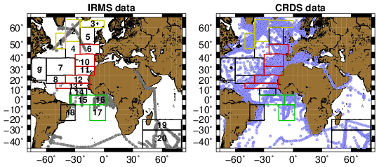
Figure 1 Maps of Wisotopes data distribution with the contours of the different regional boxes outlined with their reference number. The color of the outlines corresponds to region A (boxes 1–3, yellow), region B (red), and region C (green) (black boxes are not included in those regions). Left panel for IRMS measurements, and right one for CRDS measurements. The black dot in the western subtropical Atlantic in the right panel marks the BATS station site. A large number of plotted data points are associated with more than one data point, for example when they correspond to repeated cruises, often happening at the same time of year (cf. seasonal maps of data density in Appendix A).

The validation steps, as well as the large percentage of surface data points mostly in the open ocean in the CISE-LOCEAN database (close to 9000 validated δ¹⁸O near-surface data associated with a valid salinity since 1998) represent significant differences with respect to other published data compilations such as the “GISS Global Seawater Oxygen-18 Database – V1.21” for seawater stable isotopes which does not include the CISE-LOCEAN data (LeGrande and Schmidt, 2006; referred to as GISS-V1.21), or the CoralHydro2k seawater database, which includes an earlier version of the CISE-LOCEAN data (Atwood et al., 2026). GISS-V1.21 is a compilation of different individual data sets covering several decades originating mostly from ocean cruises and measured by IRMS, for which there was an attempt to correct systematic biases between data subsets, but that includes fewer surface data points. The CoralHydro2k data base does not offer systematic correction of potential biases between different datasets, but it contains significant metadata that could be used for further evaluation. Furthermore, the large proportion of surface data produced by CRDS in the LOCEAN database (close to 80 % of the surface data) offers the opportunity to investigate δ²H and d-excess, in addition to δ¹⁸O, these two other variables being much less frequent in the GISS-V1-21 archive.

Originally, the samples in the CISE-LOCEAN database were mostly collected during research cruises, often repeated in different years for the same season, as well as on board ships of opportunity with collection by a LOCEAN-recruited ship rider (Benetti et a., 2017a), quite commonly in the North Atlantic subpolar gyre (Reverdin et al., 2018). More recently (mostly since 2018), the database also incorporates samples collected on vessels of opportunity (VOS) by a mariner or a sailor, which often involves a later transfer from a salinity bottle to a dedicated vial. Although these VOS data tend to present less consistency, we retain them in the database, because they are the only source of data in most tropical-subtropical areas and in some seasons. The resulting data distribution is quite skewed towards better sampling in the northern to equatorial Atlantic Ocean and nearby seas, the south-western Indian Ocean and between Tasmania and Antarctica (Fig. 1). Even in these regions, except in the NASPG, there are usually seasons with very limited or no sampling: for example, during boreal summer in the equatorial Atlantic, austral fall in the southwestern Indian Ocean, and late boreal fall to early spring south of Tasmania (Appendix A). Because of insufficient data availability during a large part of the year, we will not present results for the region south of Tasmania, as well as other world regions, which are less-well sampled in the CISE-LOCEAN database. Although IRMS surface δ¹⁸O data are less common, they still contribute significantly to the sampling in some regions and seasons (e.g. equatorial Atlantic in boreal summer, southwestern Indian Ocean in boreal winter; see Appendix A).

Independently of the CISE-LOCEAN database, we also considered surface samples collected mostly monthly, close to the BATS hydrographic site (31°50^′ N, 64°10^′ W) from 2015 to 2022. These samples were conditioned in plastic bottles, frozen and stored at the University of Bergen (Norway) before being analyzed in 2023. They were again unfrozen in November 2025 to be transported to LOCEAN where they were analyzed a second time between 5 December 2025 and 11 January 2026 on a CRDS unit which experienced a set of technical problems reducing the accuracy. There are also indications that some of the samples had evaporated (5 samples in the Bergen analyses, and 19 samples in the LOCEAN analyses). This is due to the plastic bottles not being completely proofed against air exchange when closed and not frozen.

2.2 Methods

We aim at a finer scale analysis of Wisotopes than in LeGrande and Schmidt (2006) where most of the surface North Atlantic is included in one single region, when considering their relationship to salinity. Indeed, this should be viewed as a continuation of Benetti et al.'s (2017) regional analysis, as well as water mass analyses such as in Frew et al. (2000) and Voelker et al. (2015), but with strict focus on the surface (top 10 m). We consider boxes bound in latitudes and longitudes (Fig. 1), in which only samples with a salinity within specified ranges (later reported in Table 1) are retained to avoid the freshest waters directly influenced by strong local freshwater inputs (rivers, heavy rain events, large sea ice melt) which can lead to very skewed salinity distributions (Bingham et al., 2002), and possibly different relations between salinity and Wisotopes.

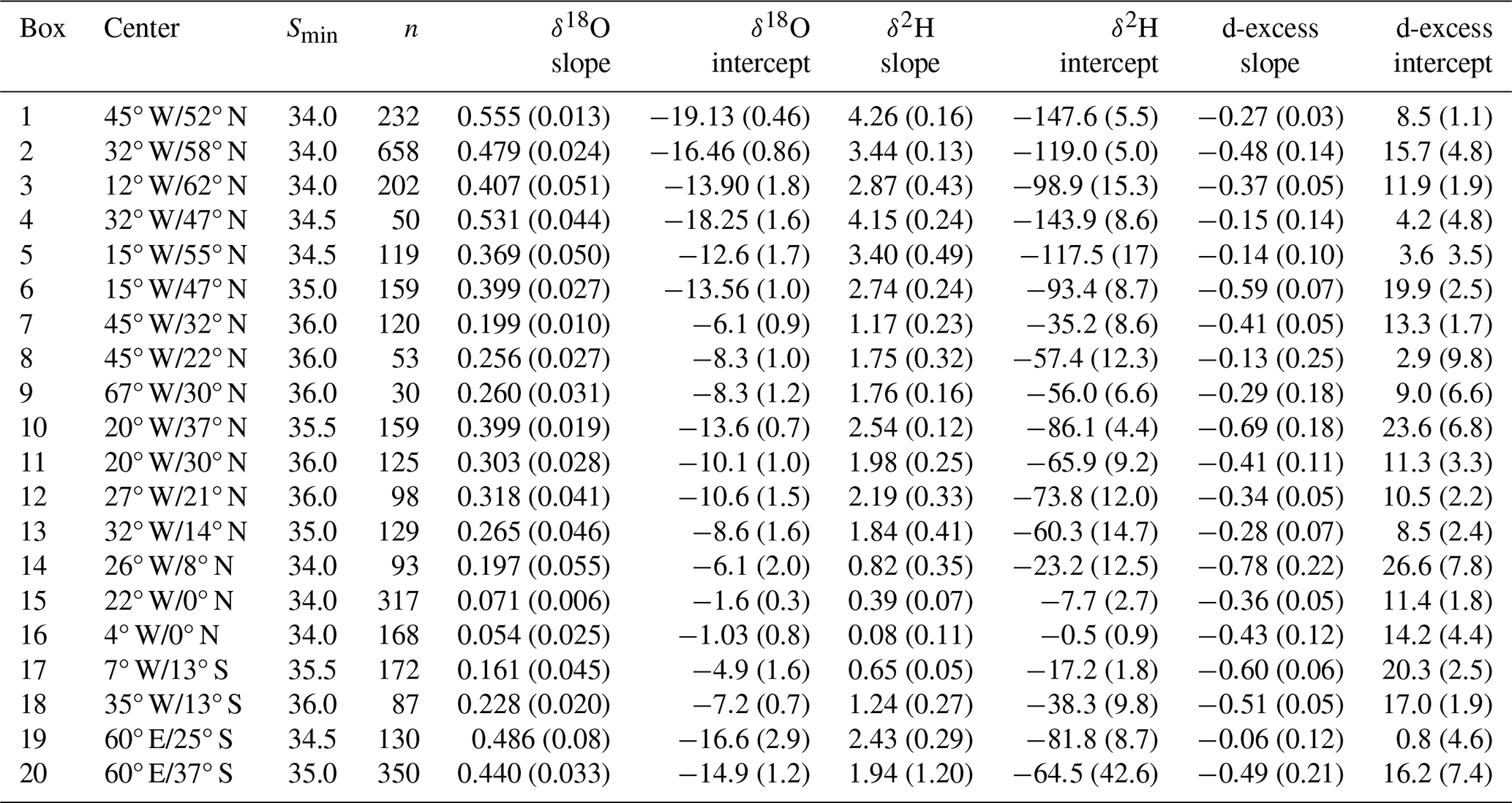
Table 1 Annual averages of the slopes (‰ per pss) and 0-intercepts (‰) of Wisotopes as a function of S in the different boxes. Left for δ¹⁸O, middle for δ²H, and right for d-excess. These averages (and their standard error in parentheses) are obtained by arithmetically averaging the linear regression coefficients obtained for the seasons with data. The minimum salinity threshold (S_min) as well as the total number of data points (n) are also reported.

The regional boxes correspond to identifiable oceanographic domains with respect to ocean circulation, as well as to specific regimes of the air-sea exchange – by Evaporation (E) and Precipitation (P) –, or to other freshwater sources. In practice, the boxes must in general be relatively large in order to retain data throughout the seasonal cycle. Despite that, except in the NASPG (boxes 1 to 3), there is often at least one season much less sampled than the others.

In each region, horizontal and vertical mixing between different water masses and their advective paths, as well as freshwater inputs and evaporation result in a spread of surface salinity, as well as in Wisotopes. Sometimes the different water masses are not isotopically distinguishable in a [Wisotopes, salinity] diagram. For example, in the equatorial Atlantic and eastern subtropical gyre of the Atlantic Ocean, Benetti et al. (2017b) could not distinguish the signatures of upwelled waters from the ones of the surface water masses advected from higher eastern subtropical latitudes.

To resolve the seasonal cycle of Wisotopes, it is useful to establish regional monthly relationships between Wisotopes and S. In principle, the better-defined monthly fields of salinity could then be used to reconstruct spatial fields of Wisotopes, as was done in LeGrande and Schmidt (2006) with large-scale annual linear relationships. However, to partially circumvent the issue of insufficient isotopic sampling, the compromise adopted here is to group in each box the data into four quarters (months 1–3, 4–6, 7–9, 10–12), which, as will be presented in the results section, sometimes produces too uncertain seasonal linear regressions. Thus, to investigate whether systematic seasonal differences in these linear relationships can be identified, we also averaged the seasonal relationships of nearby boxes in larger regions (regions A, B, C on Fig. 1).

The data were not numerous enough to investigate possible non- linearity in the relationships, especially within the restricted salinity range retained. The linear regression of Wisotopes as a function of S are obtained with least square means in the [S, Wisotopes] space, thus minimizing non-explained residual variance in Wisotopes. To reduce the influence of less common data at the lowest or highest salinity tails of the distribution, we also estimate a slope and 0-intercept (value of the regression line at S=0) by directly fitting the averages of two classes of data, one for the data below and one for the data above the seasonal salinity average.

The comparison of the two approaches indicates that the unbiased, but slightly noisier second approach often leads to a significantly larger slope. In the four North Atlantic subpolar gyre boxes (1, 2, 3, 4), this excess slope averages ∼4 %, 6 %, 10 % of the mean slopes for δ¹⁸O, δ²H and d-excess, respectively, whereas these increases tend to be smaller in the eastern mid-latitudes and northern tropics. The differences are usually largest for d-excess, and always within the uncertainty estimates of the slopes in individual regions. Thus, for simplicity, we will only report the second estimate in the results section.

We then average the seasonal linear relationships between Wisotopes and S to obtain annual-averaged linear relationships. The advantage of this approach is that the different seasons are given similar weight, avoiding thus an impact of seasonal sampling bias when estimating the annual-averaged relationships. The caveat is that the resulting uncertainty on the average can be strongly influenced by less well sampled, more uncertain seasons.

In each box, the isotopic data were also averaged by month to estimate a seasonal cycle, with unresolved spatial or interannual variability in the sampling contributing to the standard deviation between data points. The climatological monthly salinity fields present spatial gradients in each region, which likely also imprint on the Wisotopes fields, assuming a quasi-linear relationship with respect to salinity. With a limited and spatially inhomogeneous discrete sampling, this contributes to a representativeness error on the monthly mean of the discrete samples. This error can be large, as can be guessed from the seasonal sampling distribution plotted in Appendix A, with monthly sampling ranging from less than 4 samples (in more than half the month-boxes averages) to over 100. We estimate the effect of limited spatial sampling in Appendix B using two climatological products for years including a good part of the isotopic data (described in Reverdin et al., 2007 and Boutin et al., 2016, 2021). We also estimated a spatial representativeness error on Wisotopes, using the estimated linear regression of Wisotopes to the salinity representativeness error.

As discussed in Appendix B, in most boxes and for a large part of the seasonal cycle, the spatial standard deviation of climatological monthly salinity contributes to a rather large representativeness error which often exceeds 0.1 on salinity within the CISE-LOCEAN dataset. For example, in the central equatorial Atlantic (box 15 on Fig. 1), sampling in specific months (in particular March) (see Appendix A) is from repeated cruises along dedicated tracks resulting in a strong deviation of the average salinity of the discrete data points from the domain-average salinity. The month-to-month changes in sampling thus strongly contributes to the estimated box-averaged salinity seasonal cycle. The expectation is that this would also be the case to some extent for the Wisotopes, which was tried by using the seasonal or annual-averaged linear relationships of Wisotopes to salinity to adjust for this effect. The notable exception, where the spatial representativeness error is not a major issue, is the three more regularly sampled boxes of the North Atlantic subpolar gyre (1, 2, 3 on Fig. 1), where the seasonal cycle is, however, relatively weak.

3 Results

3.1 Annual-averaged linear regressions

For more than half of the boxes, the uncertainties on the individual seasonal slopes (and 0-intersects estimated by the extrapolation of the regression line to S=0) are larger than the differences between these seasonal values. Portraying the spatial variability in the slopes and 0-intersects of the individual boxes is thus not feasible at the seasonal time scale. Thus, we will only illustrate this spatial variability for the annual-averaged regressions in each box. In order not to bias the average because of uneven sampling across seasons, we retain all seasonal estimate that are based on at least 4 data points originating from at least 3 separate years. On the other hand, we still retain seasons with very small sampling which can induce large standard errors on the annual-averaged coefficients (such as in regional boxes 5, 8, 9, 17, cf. Appendix A). In boxes 19 and 20 (SW Indian Ocean), these annual averages are obtained by averaging only three (δ¹⁸O) or two (δ²H and d-excess) seasons, respectively, as the other seasons have no data.

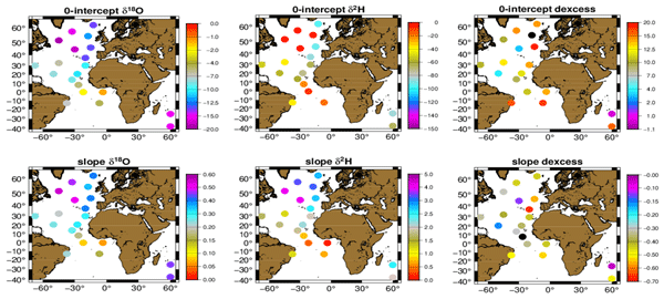
The average slopes of δ¹⁸O and δ²H as a function of S (Fig. 2, Table 1) are largest in the northern and western NASPG (boxes 1 and 2 in Table 1), as well as in the South Indian Ocean (boxes 19 and 20), whereas they are smallest near the equator. Slopes are usually also a little smaller in the western subtropical North Atlantic than in the eastern part. The 0-intercepts patterns mirror the patterns of the slope (with the opposite dependency: most negative in northern NASPG and south Indian Ocean).

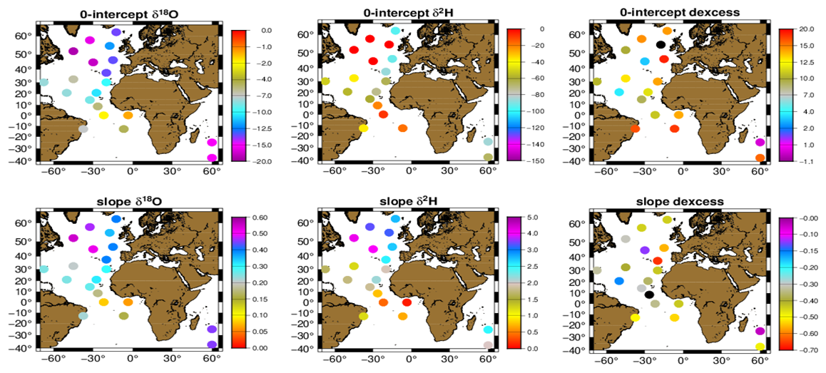
Figure 2 Annual averages of the slopes (‰ per pss) and 0-intercepts (‰) of Wisotopes as a function of S in the different domains. Left for δ¹⁸O, middle for δ²H, and right for d-excess (cf. Table 1 for standard errors on these averages, estimated from the dispersion between the different seasonal averages).

For d-excess, the pattern is less clear with larger relative errors, in particular for some of the most extreme values (Table 1). Negative slopes are however larger in the three tropical Atlantic boxes off the equator (14, 17, 18) compared to the equatorial boxes (15, 16), and are smaller just south of the NASPG (boxes 4 and 5), as well as in box 19 in the subtropical South Indian Ocean near 25° S. The d-excess 0-intercepts present a similar pattern to the one in the slope, with large positive 0-intercepts for large negative slope values. The overall anti-correlation of slope and 0-intercept may arise from noise in the dataset, as S=0 is very far from the range of salinity in which data were retained, and thus an extrapolation based on a noisy slope estimate would induce an anti-correlated noise in 0-intercepts.

3.2 Seasonal linear regressions in well-sampled regional boxes (NASPG)

In the particularly well-sampled box 2 (Irminger Sea and nearby areas), the residuals of individual data points with respect to the seasonal linear regression have a standard deviation of 0.048 ‰, 0.35 ‰ and 0.21 ‰ for δ¹⁸O, δ²H and d-excess, respectively (averaged over the four seasons). In this box 2, which does not present a large spatial or temporal variability in salinity, a significant share of the variance of the individual data in a given season is explained by the mean linear regression to S for δ¹⁸O, δ²H (Pearson correlation coefficient r averaged over the four seasons of 0.69 and 0.67, corresponding to correlations which are always significantly different from 0 at p=0.01), but not so for d-excess (r=0.35). Similar significance levels are found in the nearby boxes 1 and 3 in the NASPG, with caveats of slightly larger uncertainties due to somewhat weaker sampling in some season. This encourages us to check whether there are seasonal differences in the regressions.

The seasonal distributions of the linear fits of Wisotopes to S are illustrated for two rather well sampled boxes in the western and north-central NASPG (1 and 2 on Fig. 1) (Fig. 3). The average salinity cycle roughly corresponds to what is expected in these two regions (Reverdin et al., 2018) with lower summer-fall salinity and higher winter-spring salinity. In both regions the different seasonal distributions for δ¹⁸O, δ²H versus S!nearly overlay each other with maybe a small negative isotopic shift in months 10–12 contrasting with a positive shift in months 7–9, at least for the westernmost region. There are also slightly larger slopes in months 1–3.

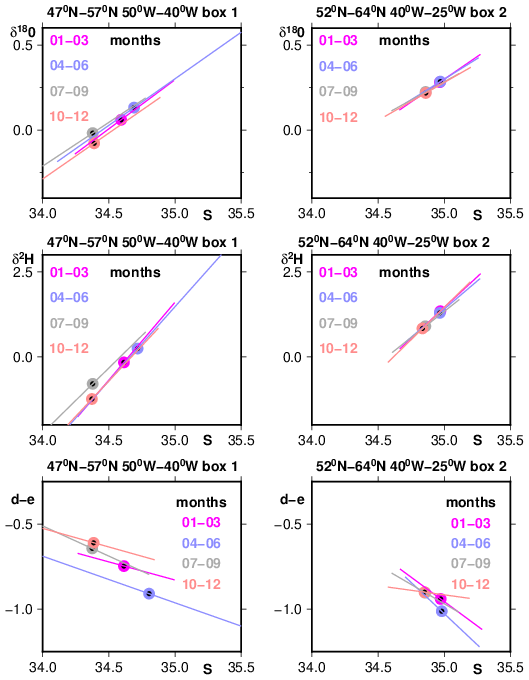
Figure 3 Seasonal linear fits of Wisotopes (‰) versus S (from top to bottom for δ¹⁸O, δ²H and d-excess) for two boxes (1 and 2 on Fig. 1) which are part of region grouping A in the north-western and central North Atlantic subpolar gyre. Data have only been retained for S within 34 to 35.5 and the linear fit is provided within the seasonal S range observed. The dots correspond to the averages, with their standard error always within the plotted dots for these two well sampled regions (for box 1, the seasonal data number varies between 26 (months 4–6) and 77 (months 1–3); whereas in box 2, it varies between 102 (months 1–3) and 225 (months 7–9)).

The seasonal d-excess versus S distribution also suggests differences according to the seasons, with d-excess apparently shifted to lower values in the spring season (4–6). The d-excess deviations across seasons exceed the uncertainty on the averages. For instance, assuming that all data points provide independent realizations, the standard errors on the d-excess averages in season 4–6/7–9 are respectively 0.04/0.03, and 0.015 ‰/0.016 ‰ for the western and north-central regions of the NASPG (1 and 2 on Fig. 1), respectively. This is supported in a nearby region (3) south-east of Iceland with reasonable sampling (not shown). There is also a suggestion of a lower slope in season 10–12 with slopes altogether lower in the western than in the central NASPG (1 and 2 on Fig. 1). However, the estimated standard errors for these d-excess versus S seasonal slopes are large and are estimated to be on the order of 0.15 ‰per psu in all seasons. Thus, even in these well-sampled regions, the differences between seasons in the slope of d-excess versus S linear relationships are within the error bars.

3.3 Seasonal linear regressions in larger regions

Except for the well-sampled boxes in the NASPG, uncertainties are often large on seasonal regressions, in particular when sampling includes less than 10 individual data points, in particular for d-excess. For this derived variable, this is due to a worse noise/signal ratio, with a smaller proportion of the variability explained by the regression to salinity. These proportions vary between boxes, but for δ¹⁸O, δ²H the part of the variance explained by the linear regressions tends to decrease towards the lower latitudes. The lowest values (20 %–30 %) are near the equator, thus corresponding to correlations which are only significantly different from 0 at p=0.02 or 0.05. On the other hand, for d-excess, the linear fit holds best in the equatorial Atlantic boxes where it explains on the order of 40 % of the variance in individual data points (r of 0.63 significant at p=0.01).

Thus, in order to retrieve a significant seasonal signature in the slopes and 0-intercepts, one needs to reduce the impact of the limited sampling on the seasonal uncertainties. To do that, in each season, we average the regression estimates for individual boxes into larger domains, based on commonality in the sources of water, and whether evaporation dominates over precipitation and other meteoric waters or the opposite. In particular, we identify three regions. Region A groups boxes 1 to 4 in the North Atlantic subpolar gyre (yellow boxes in Fig. 1), with usually excess precipitation, a freshwater input from the Arctic and potential contribution of sea ice melt. Region B extends from mid-latitudes to northern tropics in the eastern Atlantic, encompassing 5 boxes (6, 10 to 13, red in Fig. 1), with usually excess evaporation and limited local continental meteoric inputs. Region C is an equatorial and south-equatorial region grouping 3 boxes (15 to 17; green in Fig. 1), sharing an upwelling season, another season with excess precipitation, and possible influence of continental meteoric water. We also attempted to create a western subtropical Atlantic region, and to separate the northern tropics from the more northern mid-latitudes in the eastern Atlantic. However, the uncertainties were then too large in some seasons for these smaller regions, so that we discarded such groupings.

These regional composites (Fig. 4, Table 2) do not show large/significant seasonal variability of the slopes/intercepts, but there are some hints of signals. For example, in northern region A (yellow on Fig. 1) for δ¹⁸O, the slope is slightly higher and intercept more negative in season 1 than during the rest of the year, albeit the difference is not significant at the 90 % confidence level (Fig. 4). On the other hand, Table 2 for d-excess in region A indicates a more negative slope and a larger 0-intercept in season 2, and the opposite for season 4, but these differences are also barely significant at the 90 % confidence level. Furthermore, these extrema happen for different seasons than for δ¹⁸O.

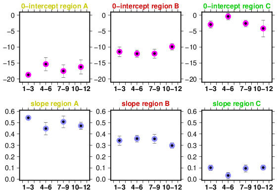
Figure 4 Slopes (upper panels, in ‰ per psu) and 0-intersects (lower panel, in ‰) from the seasonal regressions of δ¹⁸O versus S in the three regions reported in Table 2. The dots are the averages with added standard error bars. From left to right: region A for the North Atlantic sub-polar gyre (yellow boxes in Fig. 1), region B for the eastern North Atlantic (red in Fig. 1), and region C for the equatorial Atlantic south of 5° N (green in Fig. 1).

Table 2 Domain-averaged seasonal slopes and 0-intersects (standard error in parenthesis) from the regressions of Wisotopes versus S (region A for the North Atlantic Sub-polar gyre, B for the eastern North Atlantic, and C for the equatorial Atlantic south of 5° N. Seasons 1 to 4 are respectively for months 1–3, 4–6, 7–9, and 10–12. Note that for region 3, season 3, there are not enough data points in δ²H and d-excess, and in season 4, region 17 is not included in the average values for δ²H and d-excess. Units are ‰ per pss for all slopes and per mil for all intercepts.

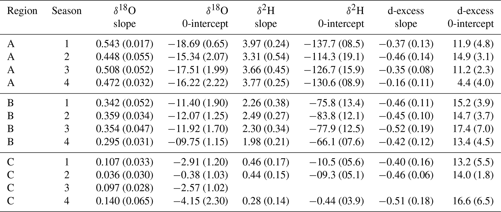
In region C (equatorial Atlantic south of 5° N, green in Fig. 1), the slope for δ¹⁸O is lower and the 0-intercept less negative in season 2 than during the other seasons, differences also barely significant at the 90 % confidence level. On the other hand, there is no significant seasonal signal in the composite for region B (eastern Atlantic, red in Fig. 1).

3.4 Monthly time series

In most regions, monthly standard errors are often large compared to the amplitude of the seasonal cycle, and part of the apparent seasonal cycle results from spatial sampling biases. However, there are a few regions where there is sufficient agreement in the salinity seasonal cycle with the climatology, such as in the central and western parts of the NASPG, or in the central Atlantic box 14 (5–12° N) (cf. Appendix B). The sampled S seasonal cycle in this last region presents a good agreement with monthly salinity climatologies, whereas in box 15 to its south (5° S–5° N) there are larger differences, in part because of large month-to-month spatial differences in the sampling (cf. Appendix B). We thus chose to illustrate the average seasonal cycles for surface salinity, δ¹⁸O, δ²H and d-excess in these two contrasting equatorial regions with the monthly means and the standard deviations of the monthly samples (Fig. 5). In addition, the smaller estimated standard errors are commented in Appendix B for these two regions. For the equatorial region, we also estimate a seasonal cycle in Wisotopes free of the spatial sampling bias, based on the expected S-bias (from Appendix B) and the annual S-Wisotopes linear relationships of Table 1.

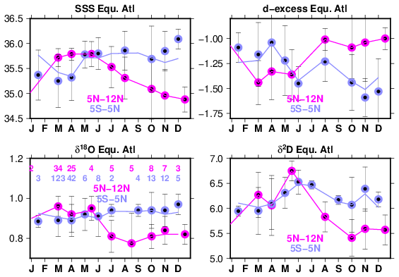
Figure 5 Average seasonal cycle in two central equatorial Atlantic boxes (14 and 15) for S (practical surface salinity, with no unit), δ¹⁸O, δ²H and d-excess (in ‰). The averages are usually provided monthly, except bi-monthly in a few instances with insufficient monthly sampling. The standard deviation among the data points is plotted (as ±1σ), and the monthly data number indicated for δ¹⁸O lower left panel. For the 5° S–5° N box 15, the blue curves are estimated box-average seasonal cycles after removing the spatial sampling bias (Appendix B).

The two boxes of Fig. 5 present a large contrast in the seasonal cycles. The seasonal cycles in the 5–12° N box have a much larger amplitude than the ones in the 5° S–5° N box, especially after the correction applied to remove the spatial sampling bias. In the 5° S–5° N box, the standard deviation of the seasonal cycles diminishes when applying the S-derived sampling bias correction from 0.27 to 0.15 for S, 0.027 ‰ to 0.015 ‰ in δ¹⁸O, from 0.19 ‰ to 0.16 ‰ in δ²H and from 0.19 ‰ to 0.14 ‰ in d-excess. Furthermore, the correlation coefficients between S and other Wisotopes variables diminishes when applying the spatial bias. They remain significant at the 90 % confidence interval for δ¹⁸O (Pearson correlation coefficient of 0.71), but not so for δ²H (0.60) or d-excess (−0.46, compared to −0.78 before removing the spatial bias). The lack of correlation for d-excess is not surprising given the estimated standard errors (cf. Appendix B) and the very limited sampling in particular in months 7009. In the 5–12° N box, the correlations with S are more significant for δ²H (Pearson correlation coefficient of 0.88) and d-excess (−0.87), but not for δ¹⁸O (0.73).

As a complementary vision on what these box-average seasonal cycles entail, the different seasonal averages are plotted with the annual average regression lines from Table 1 in Wisotopes versus S (Fig. 6). For δ¹⁸O, δ²H, they nearly overlay the regression lines, suggesting that the seasonal changes mostly correspond to the action of similar hydrological processes as the spatial spread during one season. However, this is somewhat different from the larger regional averages from Fig. 4 and Table 2, which include the 5° S–5° N box and suggest a seasonal cycle of the slopes and 0-intercepts. This thus requires a little bit of caution on how spatially stable these relationships are within the larger region C, and whether the processes that control the spread of sampled values are the same as those controlling the regional average. Notice also that there is a suggestion of a seasonal difference in d-excess with points in seasons 4–6 and 7–9 (10–12, 1–3) to the right (left) of the average regression line for both regions (Fig. 6).

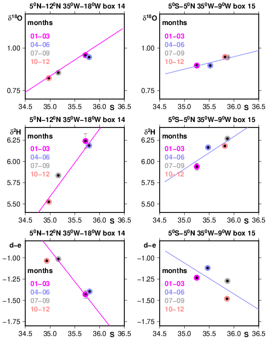
Figure 6 Average linear regressions of Wisotopes (‰) as a function of S (the average of the four seasonal linear regressions) from Table 1 (boxes 14 and 15) for two central Atlantic equatorial regions (left 5–12° N; right 5° S–5° N) displayed from top to bottom for δ¹⁸O, δ²H and d-excess (d, e). The four average seasonal values (without correction for the spatial representativity error) are shown with their standard error bars (SE) (it is smaller than the dots size, except in season 1–3).

In most other regions, the seasonal cycle in salinity and Wisotopes is rather weak or presents large uncertainties, with the exception of three better-sampled boxes in the North Atlantic subpolar gyre. We also present in Appendix C, the seasonal cycle of the BATS time series monitored over 7 years. As there is regular sampling at that site, there is no spatial representativity error to correct. Standard errors come from the meso-scale and interannual variability, as well as poor sample conservation and measurement uncertainties (see discussion in Appendix C). A comparison was done with box 9 results, but this box is the least well-sampled box and spatial representativity errors are large. Nonetheless, at 0-order and with standard errors comparable to the observed seasonal cycle, box 9-values agree with what is obtained at the BATS station.

4 Discussion

4.1 Annual-averaged linear regressions

Although this dataset is not always sufficient to identify seasonal variability in the relationship of Wisotopes with salinity, it allows to portray rather well the spatial structure of these regressions, and with little seasonal bias. This usually fits well with what was published earlier. Frew et al. (2000) indicate for the NASPG a rather steep slope of the regression line of δ¹⁸O versus salinity (0.59 ‰ per pss) and a rather low 0-intercept (−23 ‰) indicative of a large contribution of meteoric waters/freshwater of Arctic origin. These values are close to but a little larger with respect to the ones we find in the surface waters. Our data are mostly located in the western part of the NASPG, and exhibit a smaller spread? Part of the difference originates in that we do not retain the lowest salinities typical of the shelves and slopes in the regressions. The surface data in Voelker et al. (2015) a little further south (30–40° N) in the eastern Atlantic indicate for δ¹⁸O a somewhat lower slope (0.32 ‰ per pss) and a higher 0-intersect, somewhat similar to what we find in collocated boxes 11–12 (similar agreement found for δ²H).

Benetti et al. (2017a), who also reports on δ¹⁸O, δ²H and d-excess from a subset of the data used here, show spatial variability in the regression line of Wisotopes with salinity between some of the same regions of the mid-latitude to equatorial Atlantic that are explored here with a widely extended dataset. Benetti et al. (2017a) explained to some extent the spatial variability from mid-latitudes to the equator through properties of P and E, and the relative contribution of the two, with for example the central equatorial Atlantic dominated by precipitations not very depleted in heavy isotopes, thus inducing a small slope in the distributions of δ¹⁸O, δ²H, to salinity. They additionally present an east to west contrast in the slopes at the North Atlantic tropical and subtropical latitudes. They point out that the surface water masses in the western Atlantic carry the advected contribution of the Amazon-Orinoco discharge and low latitudes precipitations, whereas the surface water masses in the eastern Atlantic advect high latitude North Atlantic contribution as well as excess evaporation. Our study also finds that contrast, and suggests that this is not related to seasonal differences in the sampling used in Benetti et al. (2017a), albeit sampling in the western subtropical Atlantic is sparse. Furthermore, the lowest regression slope for δ¹⁸O and δ²H in the western subtropical North Atlantic is also supported by the BATS hydrographic station surface data (see Appendix C).

4.2 Seasonal linear regressions

None of the earlier papers nor the mapping presented in LeGrande and Schmidt (2006) discuss the seasonal variability in surface Wisotopes data in the regions investigated here away from shelves and continental slopes, because the poorer sampling and larger scatter in the earlier datasets would only allow to separate the largest spatial scales (and only for δ¹⁸0) in a “time-average way”.

To some extent, the qualified surface data in the updated CISE-LOCEAN database allow to make some step towards resolving the seasonal time scales. Sampling remains very low in large areas (Fig. 1), with often too large scatter in the data. There are some regions with large deviations in the regression to salinity: for example, west of the British Isles, the relationships are different possibly because there are multiple sources of freshwater mixing up with North Atlantic Drift waters from the subtropics: input from the fresher NASPG waters with an Arctic water input, on one hand, but also less depleted freshwater from rain and runoff from the British Isles and western Europe. Importantly, this region is insufficiently sampled, so these deviations could also be artefacts due to insufficient sampling. Similarly, in the 20–30° S band of the southwestern Indian Ocean, we also find rather uncertain seasonal regressions (Table 2). Based on Reverdin et al. (2025) (and publications therein) this could originate from a combination of two main freshwater sources to this mostly excess-evaporation region: a first one very depleted which is advected from the surface sub-Antarctic austral ocean with southern latitude characteristics, and a second one less depleted carried by the Indonesian throughflow from the western equatorial Pacific and maritime continent to the southwestern tropical Indian Ocean. In the present study, we have not tried to separate the two and could not test whether there is a seasonal dependence in the respective contribution of these two water masses.

In the central equatorial Atlantic, when comparing the Wisotopes averages in the 5–12° N (box 14) with the ones in the 5° S–5° N (box 15), we find well defined seasonal cycles in both regions, albeit with very different timings of maxima and minima (Fig. 5). This is expected from the seasonal meridional displacements of the Inter-tropical convergence Zone (ITCZ) and associated changes of ocean circulation and equatorial upwelling, as discussed for S (Reverdin et al., 2007; Da-Allada et al., 2013; Yu et al., 2021). The ITCZ is furthest south in January-March, with a later initiation of the seasonal equatorial upwelling in May, simultaneous with the northward displacement of the ITCZ, as well as the setting of the eastward North Equatorial CounterCurrent (NECC) later on (July–August) bringing water from the Amazon plume in addition to local precipitation to the central equatorial Atlantic further north (box 14, 5–12° N). This would have induced in season 10–12 of box 14 (5–12° N) changes in δ¹⁸O and δ²H intercepts (Fig. 6), and a lower intercept for d-excess (not shown) compatible with a seasonal influence of Amazon river discharge (properties of waters more strongly influenced by Amazon discharge are presented in Benetti et al., 2017a). In each of the two regions, S, δ¹⁸O and δ²H vary mostly in phase, whereas d-excess varies in opposite phase (but not significantly in box 15, 5° S–5° N) (Fig. 5), consistent with the average regression of these different properties with respect to salinity (Table 1).

In the north-western Atlantic (boxes 1 and 2 of Fig. 1; but this also holds for nearby regional boxes included in region A of Table 2), one finds in winter (months 1–3) a larger regression slope (and more negative 0-intercepts) for δ¹⁸O and δ²H than in other seasons. This is reminiscent of the results in Benetti et al. (2016), which they attribute to an upstream contribution of sea ice formation (brine release), albeit we restrict here the data to salinities above 34, thus possibly missing a good part of this signal, which is strongest at the lowest salinities and along the shelves and continental slopes. Interestingly, for d-excess, the largest anomaly happens less in winter than in spring, with the average d-excess and individual data points shifted to more negative values (at constant S), and with a larger negative slope (at least when averaged over the four seasons, as presented in Table 1, and seasonally grouped as region A in Table 2) and a larger positive 0-intercept. It would be tempting to relate that to advection of water affected by sea ice formation processes. However, the respective fractionations for δ¹⁸O and δ²H when sea ice forms, at least at equilibrium, remain very close to a ratio of 8 in Souchez et al. (1988), thus inducing no major change for d-excess in the remaining liquid sea water. Thus, as salinity increases due to brine releases, the regression line would shift to the right in a d-excess versus S diagram, thus above what on Fig. 3, whereas the opposite is observed. As these are areas with active winter air–sea exchange and mixing of the upper water column, although not to the same level in the four regional boxes, the changes might also be attributed to those processes. This would require a modelling approach to fully apprehend.

In most other regional boxes investigated, the seasonal differences observed in the regressions to salinity were not found to be significant, even after grouping (averaging) these different regions into larger domains (Fig. 4, Table 2). Thus, the seasonal variability is usually not of a similar magnitude as the large-scale spatial differences. This thus allows for the use of the surface Wisotopes data in comparisons of different databases/sets, even if these datasets have not been collected in the same season (as done in Reverdin et al., 2025). This does not preclude that some areas with large seasonal variability of advection, evaporation (E), precipitation (P), and different sources of freshwater may present larger seasonal signals in the regional regression lines. This is probably what we observe in the central equatorial Atlantic in months 3–4, and it is also likely the case in areas of the western equatorial Atlantic presenting very large seasonal (and interannual) variability, due to the freshwater seasonal discharges mostly originating from the Amazon/Orinoco rivers. This has been observed in other oceans, such as in the western/central equatorial Pacific (Conroy et al., 2017; Horikawa et al., 2023). Higher data density would be required to establish potential seasonal and interannual variability in the regression lines. For example, in the South Indian Ocean, although there is a long time series (starting in 1998) with often adequate spatial sampling for austral summer (1–3) conditions (Akhoudas et al., 2023), there are nearly 5 months in the year with no data in the CISE-LOCEAN database, and the winter data are mostly from the beginning part of the time series, thus with the possibility of trends (Akhoudas et al., 2023) creating apparent seasonal variability.

4.3 Monthly time series

When establishing box time series with limited spatial sampling, we face the issue of spatial representativeness errors in the sampling. An attempt was done to correct it by using the annually-averaged regression lines in the same box with the estimated salinity representativeness errors (Appendix B). This resulted in reduced seasonal variance in Wisotopes in equatorial Atlantic box 15. On the other hand, there is the caveat that the larger scale seasonal regression line (domain C) shows a large seasonal variability, albeit marginally significant (Fig. 4). Using this modulation of regression line in box 15 does not significantly modify the seasonal cycle in δ¹⁸O and δ²H, with slightly lower values for months 11–12 and higher values in months 1–3 (not shown). On the other hand, with the limited sampling, there is also the likelihood that insufficiently sampled interannual to multi-decadal variability might result in a temporal representativity error. For example, in the South Indian Ocean, multi-decadal trends have been described both in the southwestern subtropical region and south of the Subantarctic front, which have been ascribed to changes in the hydrographic cycle and in particular in local E and P (Akhoudas et al., 2023).

The BATS site time series in the western North Atlantic subtropics (Appendix C) is one of the rare sites where there was a concerted effort to regularly collect data over more than 7 years. It shows a clear seasonal cycle in S, δ¹⁸O and δ²H, but less so in d-excess (Appendix C), as sampling is still too limited given the uncertainties in the measurements. Anomalizing the data by subtracting the monthly-averaged seasonal cycle removes a significant part of the variance (Fig. 7 and Appendix C). However, except for a few peak values exceeding ±0.15 ‰ for δ¹⁸O, the values are usually rather close to the estimated standard errors and possible magnitude of systematic errors in the data. Even with the one-year running mean (Fig. 7, black curves), standard errors remain large, averaging 0.026 in S, and 0.018 ‰, 0.13 ‰, 0.06 ‰ on δ¹⁸O, δ²H and d-excess, respectively.

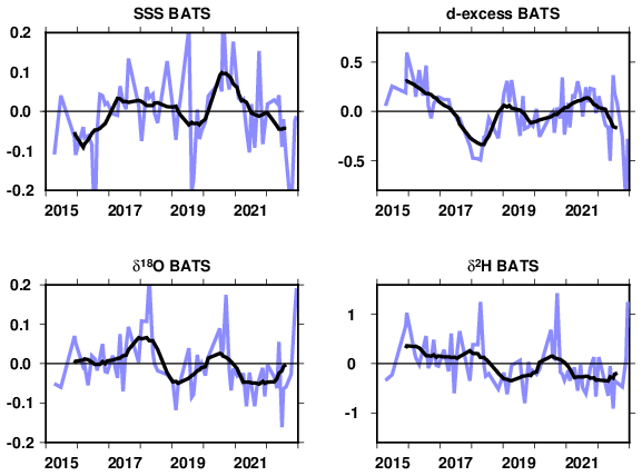
Figure 7 Anomalized time series of sea surface salinity (pss), δ¹⁸O, δ ²H and d-excess (‰) at the BATS site (31°50^′ N, 64°10^′ W). A version where averages of non-flagged LOCEAN and Bergen data is shown (see Appendix C). The blue curve connects individual data points, whereas the black curve is a 1-year running mean of the data.

Despite these large residual standard errors, the data suggest higher than normal δ¹⁸O and δ²H in, in mid-2017 to 2018 (in particular the winter 2017–2018) with lower values in 2019 and 2021. These do not seem to closely correspond to the S variability. For example, notice in early 2016 the low salinities but no low δ¹⁸O and δ²H. The d-excess time series suggests a contrast between very negative values in winter 2017–2018 and positive in 2021 as well as in late 2015 early 2016 and in 2019. This seems to partially mirror (with opposite sign) the salinity anomalies, except in 2022. These short time series appear to partially co-vary with the North Atlantic Oscillation (NAO, Hurrell et al., 2005), with the winters 2014–2015, 2017–2018, and to a lesser extent early 2020, having a positive NAO index, in contrast to 2021 with a more negative NAO index (positive NAO index associated with an increase in δ¹⁸O and δ²H, and a decrease in d-excess). A longer times series and with smaller analytical errors would allow to further explore these possible relationships, as well as other modes of climate variability.

Nonetheless, interpreting the poorly resolved interannual variability would also require model simulations, in particular to separate the effect of changes in the hydrological cycle from the effect of changes in ocean circulation or surface stratification/upwelling signals (cf. Ayache et al., 2024, but for another ocean region).

5 Conclusions

Although the current surface data in the CISE-LOCEAN database mostly collected during the last 28 years, and in particular since 2010, are still in limited number, they offer the possibility to characterize the seasonal cycle of Wisotopes and their relationship to surface salinity in part of the Atlantic Ocean and of the southwestern Indian Ocean. At 0-order in most of these regions, the data suggest that the seasonal variations of the regression of Wisotopes to salinity are not large compared to its spatial variability, and within the random and representativity errors. However, there are some significant seasonal deviations from the mean, in particular in the western North Atlantic subpolar gyre and in the equatorial region. We also find a suggestion of interannual variability at the regularly sampled BATS site in the western subtropical Atlantic.

We have only interpreted the clearest seasonal deviations from the yearly-averaged relationship in a qualitative matter. To get further would involve relating them either to changes in ocean circulation (both horizontal or vertical mixing), or in the water fluxes between the atmosphere, the cryosphere, sea ice, and liquid sea water. In addition to the data, this would require dedicated simulations of forced isotopically-enabled ocean models first validated by the observations (Ayache et al., 2024). In the longer term, this might also require isotopically-enabled earth system models, as the isotopic signatures of these different processes (evaporation, precipitation, continental inputs) evolve in our warming world, as well as the melt of continental glaciers and ice sheets which will imprint on the seawater isotopic composition (e.g., Oppo et al., 2007). Additionally, surface seawater isotope data provide model boundary conditions to assess model performance in isotope-enabled Earth system models (e.g. Schmidt et al., 2007; Brady et al., 2019; Cauquoin et al., 2019).

The data are still very limited in individual data sets such as the CISE-LOCEAN one, the earlier GISS Global Seawater Oxygen-18 database or the CoralHydro2k Seawater δ¹⁸O database. There is a pressing need to put together efforts for better isotopically sampling the near-surface oceans, and thus better constraining processes of the hydrological cycle. This requires active intercomparison of data from different laboratories, with precise qualification of their differences and respective accuracy (as currently performed within the SCOR working group 171 – MASIS). There is hope with ongoing efforts of data retrieval and updating databases that this might be reachable in many parts of the world oceans, despite the obstacles of systematic differences and insufficient data coverage (Reverdin et al., 2025).

Appendix A: Seasonal data distributions

The maps of data distribution (Fig. A1 for δ¹⁸O, but except for IRMs data in grey in Fig. A1, maps for δ²H and d-excess are rather similar) indicate strong inter-seasonal variability. On finds that mostly in regions where cruises were repeated over many years in a specific season (recent tropical Atlantic PIRATA cruises in months 3–4, Ovide NASPG cruises close to month 6, and most recent OISO SW Indian cruises in months 1–2). Except for the OISO cruises and a few mostly summer-time sail-boat samples (months 10–3), there are no data in the SW Indian Ocean (boxes 19, 20). In other areas, this is more random, and those boxes/seasons with virtually no data are specifically indicated on the maps (4, 5, 8, 9, 17). Data density is high (here estimated as within a 25 km radius) along repeated cruises and where there was a long-time concerted effort to collect water samples from ships of opportunity in the NASPG (SURATLANT project).

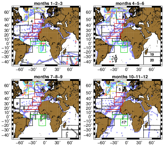
Figure A1 Seasonal data distribution with box overlain (color contours corresponding to the regions 1 – yellow, 2 – red, 3 – green). The grey dots are for IRMS data, whereas the colored ones indicate CRDS data with a color scheme corresponding to data density within 25 km of the data (blue, less than 5 nearby data, cyan with 5 to 9 data, red, 10 or more data). For each season panel, the box numbers are indicated when there are 4 or less δ¹⁸O data in the season.

Appendix B: Comparison of salinity box averages

We compare the box averages salinity seasonal cycle estimated from the LOCEAN data to climatological monthly fields of in situ salinity from Reverdin et al. (2007) updated to 1977–2016 and from the satellite-based CCI V4.4 S product averaged over 2011-2024 (Boutin et al., 2021) (later referred to as CCI). These two climatologies provide information on the effect of the limited spatial sampling in the boxes on the monthly box averages. The results with these two climatologies that differently span most of the period in which data were collected are rather similar. In most regions and for a large part of the seasonal cycle, we find that the spatial standard deviation of climatological monthly salinity contributes to a rather large representativeness error with the sampling of the LOCEAN dataset which exceeds 0.1 on salinity for most months and regions. The notable exception is in the better sampled boxes of the North Atlantic subpolar gyre.

For example, in the central Atlantic north-equatorial (5–12° N) and equatorial (5° N–5° S) domains, the spatial standard deviation of climatological monthly salinity in the in-situ climatology varies between 0.2 (north-equatorial in months 1–4) to 0.4 (north-equatorial, months 6–11) or even 0.5 (equatorial, months 10–11–12–1), and this both for the in situ and the CCI monthly climatologies. Assuming random spatial sampling in the current LOCEAN dataset, this would contribute to a representativeness error which exceeds 0.1 on salinity for most months.

However, there are other contributions to the standard error on the monthly averages, as a large proportion of the data can originate from a single cruise, and all data are not independent with respect to interannual, higher frequencies than monthly or spatial variability within the domain. These all contribute to the difference of S to the average climatological seasonal cycle. In the instance of the North Equatorial region on Fig. 2 (and other regions too), the LOCEAN S seasonal cycle is more irregular than in the sea surface salinity climatologies, but the differences are usually smaller than the 1σ standard deviation between all the data. They are however larger than if one assumes that all data are independent random representation of the mean (thus with a standard error $\mathit{\sigma }/\sqrt{n}$, where σ been the standard deviation around the mean). The compromise we adopt to estimate the standard error is to use as the number of degrees of freedom $n/\mathrm{2}$. We also propagate that estimate to the other parameters (Wisotopes), assuming that what is found for S is a model for the sampling issues.

Even, with that assumption, we find in regions with irregular spatial sampling that the differences in S with the two monthly climatologies are larger than the estimated standard error (Fig. B1). Part of that is associated with spatial variability of the poorly sampled mean monthly fields, as seen for the central equatorial Atlantic region 5° S–5° N (Fig. 2), when comparing (Fig. B1) the CCI climatology averaged spatially over the box (thick black line) with the climatology sampled at the position of the data points (thin black line). The thin black line there, but also to a lesser extent for the north equatorial box (5–12° N) is closer to the monthly data average, with differences compatible with the standard error estimates.

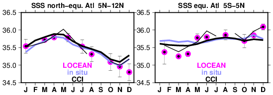
Figure B1 Comparison of average seasonal cycle in the LOCEAN dataset (dots with error bars) with two climatologies (curves), the blue one for 1977–2016 (In situ; Reverdin et al., 2007), and the black ones being for the CCI V4.4 S for 2010–2023 (Boutin et al., 2021) (the thick curve for the box averages, and the thin curve for the average at the positions of the sampling). The standard errors plotted on the LOCEAN monthly averages, are estimated taking $n/\mathrm{2}$ as the number of degrees of freedom, where n is the sample size.

In these two boxes, in months with more than 10 data points and extending that assumption to estimate standard errors for salinity to the other Wisotopes variables, the estimated standard error is small relative to the amplitude of the sampled seasonal cycle. For example, for monthly δ¹⁸O values in the equatorial domain, the estimated standard error varies between 0.01 ‰ and 0.10 ‰ (smallest in March and largest in the poorly sampled July to September) The estimated standard error is typically 6 times larger for monthly δ²H values and 4 times larger for d-excess values than for δ¹⁸O values.

Furthermore, one can also attempt to correct the sampling bias identified on salinity to the other variables, by assuming that an average linear relationship between salinity and Wisotopes holds.

Appendix C: BATS seasonal variability

Water samples were collected nearly monthly from 2015 to 2022 at the BATS hydrographic site in the western subtropical Atlantic – close to (31°50^′ N, 64°10^′ W). They were stored in plastic bottles which were frozen once arriving at the Bermuda Institute of Ocean Sciences. They were later unfrozen in Bergen (Norway) and run in three separate days on a Picarro CRDS L2130. Then, the samples were refrozen, and were unfrozen again shortly before been shipped to LOCEAN, where they were kept unfrozen at 4 °C, before analysis (thus, for some, up to nearly two months).

The BATS data have been validated and flagged as usually done at LOCEAN, based on anomalous d-excess and compared to the set analyzed at the Univ. Bergen (referred to as Bergen, later on). Out of 80 samples, some were flagged as likely bad when d-excess was deemed too low (6 for the Bergen set; 15 for the LOCEAN time series) and some as likely good but suspicious if d-excess as too high (2 for Bergen, 5 for LOCEAN). Five out of the six likely bad flagged data in Bergen were also flagged as such in the LOCEAN set, but not the two Bergen data flagged as suspicious. The larger number of flagged data at LOCEAN suggests that the plastic bottles in which the samples were stored exchanged water molecules with the outside air, after been unfrozen for shipment to LOCEAN and before analysis. The number of suspicious flags (d-excess deviating by up to +1 ‰ from usual) as well as the non-consistency for that between the two sets is suggestive of some noise in the analyses. In particular, during the LOCEAN daily runs in December 2025/January 2026 there often was a poor reproducibility of a reference sample in the runs. However, based on replicates, we expect that standard errors on the LOCEAN measurements are usually less than 0.05 ‰ for δ¹⁸O.

We also suspect systematic shifts in the Bergen set between three different days of analysis. We thus adjusted the Bergen set to the LOCEAN set by comparing unflagged data separately for each of the three days of analysis in Bergen. After that, both sets are used to estimate an average seasonal cycle (Fig. C1). Because of the small sample size (averaging on the order of 5–6 samples for each calendar month), the standard errors are large. The two sets of analyses indicate a rather coherent variability in S, δ¹⁸O and δ²H with differences within standard error bars (a mostly similar cycle is also found in the Bergen set prior to the adjustment). There are hints of a seasonal cycle with lowest S in June to September. The summer S minimum is a prominent feature in the longer BATS time series, although in the 1990–2000 decade, the minimum occurred in September (Phillips and Joyce, 2007). Figure C1 also shows lower δ¹⁸O and δ²H in June–August. Because of the limited sampling and the standard error bars, the large increase of δ¹⁸O and δ²H in September, with no counterpart in S, may not be a representative feature of an average seasonal cycle. However, it is tempting to associate it with the beginning of the tropical storm (hurricane) season in late summer, and possible individual storm/hurricane signatures. Because of the standard error bars in both analyses, we attribute better confidence in the average of the two sets of analyses (shown as the thin black line in Fig. C1), with overall a variability in Wisotopes nearly following the spatial relation between S and Wisotopes in this region, except for September (box 9 of Table 1). The standard errors are large on the d-excess monthly averages. However, the average of the two sets suggests a seasonal cycle with lower d-excess in months 12 to 5, and higher in months 7 to 10.

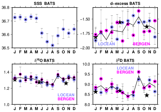
Figure C1 Monthly-averaged seasonal cycle at BATS of S, δ¹⁸O, δ ²H and d-excess (from top to bottom and left to right, in ‰) with averages for the 2015 to 2022 period and their 1σ standard errors depicted. The two colors correspond to the LOCEAN and Bergen analyses of the samples, whereas the thin line marks the average of the two sets. The black stars correspond to the averages for regional box 9 (Fig. 1) adjusted to the salinity at BATS (top panel left) taking the slopes of the regression to salinity reported in Table 2.

On Fig. C1, we also report as stars the CISE-LOCEAN data averaged in box 9 (to have enough data, months 5 and 6 were grouped, as well as months 10 and 11). These averages have relatively small standard errors on the order of 0.025 ‰, 0.160 ‰ and 0.070 ‰ for δ¹⁸O, δ2H and d-excess respectively. They seem to fit within the error bars to the curves of the BATS site, suggesting that the site is representative of a larger area.