Efficient ensemble estimation using an MCMC sampler: a reconstruction of the Mediterranean low-frequency variability combining observed and simulated sea level

The skill of climate projections depends on the ability of models to reproduce the long-term and low-frequency variability of the system. It is thus important that low-frequency model statistics can be checked against observations. In this paper, a method is proposed to estimate directly the low-frequency component of the ocean variability from native observations using statistics from a prior long-term simulation. It is designed to account for possible model biases and to provide an estimate of the correction required to fit observations. The result is obtained by an MCMC sampler (modified to include localization of the model covariance), which provides an ensemble description of the solution, so that uncertainties can be properly assessed using independent data. This algorithm is shown well suited to work with MPI and GPUs, and efficient enough to solve large-size problems (about 10⁸ variables and 10⁷ observations). The approach is illustrated by the reconstruction of the low-frequency variability of the Mediterranean sea level, using statistics from a 1/12° resolution ensemble model simulation. The resulting ensemble is assessed against independent observations (by cross-validation), showing good reliability (flat rank histogram). The method also produces a consistent estimate of the model bias and of the observation error variance (mainly representativity error), while the missing prior ensemble variance is shown to be less controlable by the observations, and thus rather computed as a diagnostic. Overall, this application shows the importance of reliable model statistics, and thus the importance of enhancing model simulations to represent all main sources of uncertainty.

1 Introduction

Climate projections depend on the ability of dynamical models to produce a reliable probabilistic description of the natural systems (mean behavior, uncertainty, extreme events, …), and on the ability of modellers to provide an appropriate probabilistic initial condition based on past data (Polkova et al., 2019; Volpi et al., 2021). These two requirements partly rely on the comparison between model simulations and observations in the context of the present climate, or more precisely within the climatic trend of the recent past. In this context, what is most important to check and analyze is the low-frequency (interannual) component of the model results.

In the context of the MEDIATION project (a French ANR project dedicated to the improvement of climate projections in the Mediterranean Sea and in the North-Western European Seas), Héron et al. (2026) produced a 30-member ensemble simulation of the Mediterranean Sea (between 1979 and 2020), with the purpose of studying the long-term dynamical response of the model to small perturbations of the initial conditions. In the present study, this ensemble simulation will be used as reference model simulation, with a focus on the low-frequency component obtained for sea surface height. Our purpose is to make a direct comparison between this low-frequency component and the available observations (along-track altimetry), and to propose an ensemble estimate of this component only by combining model results and observations. This work is a contribution to the POSYDONIE project, whose objectives is to examine how uncertainties on projections can be better described by combining simulations and observations.

To produce an ensemble estimate of the low-frequency combining the model simulations and the native observations, we will use Monte Carlo Markov Chains (MCMC) to sample the target probability distribution, which will be obtained by a Bayesian conditioning of the model probability distribution (described by the ensemble simulation) on the observations. The MCMC sampler that is used in this paper is based on the Metropolis/Hastings algorithm (e.g. Robert and Casella, 2004), using the specific variant described in Brankart (2019), which includes the localization of the prior covariance (Houtekamer and Mitchell, 1998). The method has been shown efficient enough to deal with problems of large dimension, and has already been applied to the estimation of time-dependent oceanic fields (Popov et al., 2024). In that paper, the objective was to obtain an ensemble estimate of the evolution of the ocean biogeochemical variables over one year (phytoplankton, zooplankton and a few ecological indicators) by conditioning an ensemble ocean simulation on ocean color satellite images. These observations were characterized by a very sparse time and space coverage, due to the presence of clouds masking the surface of the ocean.

A first difficulty with this approach is that our model ensemble simulation of the Mediterranean Sea has systematic errors as compared to the real world. As a result, the prior probability distribution used by the MCMC sampler cannot be solely described by the ensemble model simulation. It must be enhanced by additional free parameters to account for possible model biases. These parameters will be estimated together with the low-frequency component of the signal, thus providing a comparison between simulation and observations as a byproduct of the estimation problem.

A second difficulty is that the model ensemble simulation only provides a small sample (30 members) of the prior probability distribution. This means that only a simple statistical model can be used to describe the prior distribution, since no complex model can be inferred from a small sample. Actually, only the mean and covariance of the ensemble simulation will be involved in the construction of the prior distribution. Moreover, a localization algorithm will be applied to drop the small long-range correlations, which are unreliable because of the small sample (e.g. Houtekamer and Mitchell, 1998; Bishop and Hodyss, 2009). The resulting prior distribution will nonetheless not be Gaussian, as a result of the additional free parameters mentioned above, but still simple, and with a shape (time and space dependencies) mainly driven by the prior ensemble.

Identifying a more complex model for the low-frequency (for instance by machine learning) would have required compiling much more data than we have here. This might be possible by gathering data from many models, or by making stationarity assumptions about the statistical behavior of the low-frequency (allowing to compile data over time). However, it is not always obvious that building a complex statistical model from a large catalogue of compiled data would be more informative and reliable than a more simple model obtained from a small sample of coherent data that are more directly related to the problem at stake. Moreover, in this paper, our purpose is to be able to evaluate one particular model simulation and its ability to reproduce the low-frequency variability of the Mediterranean, to compare it to the observations (with a diagnostic of the bias) and then to determine its ability to provide an accurate estimation of the signal, together with a reliable ensemble description of uncertainties. In that context, our assumption is thus to rely on just one ensemble model simulation spanning the same period as the observations (using a realistic atmospheric forcing), with the perspective that it can be progressively improved, following future model enhancements.

In accordance with this roadmap, the objective of this paper is to propose an ensemble method to solve efficiently this type of estimation problem, and to illustrate the approach by estimating the low-frequency variability of sea surface height in the Mediterranean Sea. Special care will be taken to demonstrate the technical feasibility and potentiality of the approach, to illustrate the importance of consistent and reliable prior data, and to assess the reliability and accuracy of the ensemble estimate (including uncertainties). The code that has been used in this study is openly available, as well as the ensemble data that are produced and analyzed.

The paper is organized as follows. We first describe in Sect. 2 all data that have been used (from observations and models). Then, we present the estimation problem in Sect. 3 and the iterative Monte Carlo method that is applied to compute the solution. In Sect. 4, we describe the ensemble experiments and evaluate the results. And finally, in Sect. 5, we check the ability of the method to provide appropriate estimates of auxiliary statistical parameters (model bias, missing model variance, observation error variance). An Appendix is also included to provide a more technical description, including an analysis of the computational complexity and efficiency with MPI and GPUs.

2 Observations and model ensemble data

The solution of the estimation problem is obtained by combining observed and simulated data. Model data are used to construct a prior statistical model to be constrained by the observations. In this section, we first present all data that are used in the rest of the paper.

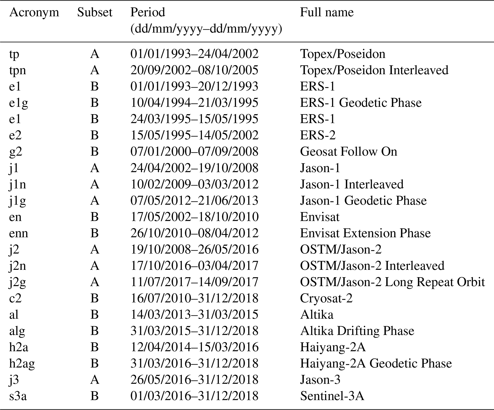
Table 1 List of altimetric datasets used in the estimation problem. The period is limited to what is actually used from each mission (between 1 January 1993 and 31 December 2018).

2.1 Altimetric observations

We use along-track altimetric data (L3 product) available between 1993 and 2018, as downloaded from the Copernicus Marine Environment Monitoring Service (CMEMS, product SEALEVEL_GLO_PHY_L3_MY_008_062). This embeds data from 12 satellite missions, organized in 21 data sets, as detailed in Table 1. For validation purpose, to keep independent observations that are not used in the estimation, we have divided this dataset in two subsets (A and B) as mentioned in the second column of the table.

The variable that is used from these datasets is the absolute dynamic topography. It is computed as the sum of the mean dynamic topography (obtained from a combination of gravimetric satellite missions, and interpolated along-track data) and the sea level anomaly (obtained from the satellite missions listed in Table 1). In this product, corrections are applied to sea level anomaly to remove long wavelength errors (e.g. orbit errors), atmospheric errors and the ocean tide (internal and external).

For comparison purpose, we will also use mapped altimetric data (L4 product) which correspond to CMEMS product SEALEVEL_GLO_PHY_L4_MY_008_047. The maps are daily and have been produced by objective analysis using the along-track altimetric data described in Table 1.

2.2 Ensemble model simulation

As model data, we use the 30-member ensemble simulation of the Mediterranean described in Héron et al. (2026). It is based on the NEMOMED12 configuration of the NEMO ocean model (Beuvier et al., 2012), implemented over the Mediterranean basin at 1/12° resolution and over 75 vertical levels, and driven by specified forcing between 1979 and 2020. The surface forcing is provided by the new ALDERA3 dataset (Nabat et al., 2020), which consists in 3-hourly air-sea fluxes (wind stress, heat and freshwater fluxes), together with a Newtonian relaxation of sea surface temperature to maintain thermal stability (with a restoring coefficient equivalent to 40 W m⁻² K⁻¹). River runoff is prescribed at the river mouths and along the coastline as a surface freshwater flux, using a 1980–2017 climatological seasonal cycle derived from the interannual dataset of Ludwig et al. (2009). Boundary forcing in the Gulf of Cadiz is applied in each ensemble member within a buffer zone, where the model temperature, salinity and SSH fields are relaxed towards their monthly climatological counterparts extracted from the ORAS4 global ocean reanalysis (Balmaseda et al., 2013), with a relaxation time scale decreasing westwards. More details and references about the model configuration can be found in Héron et al. (2026).

The simulation starts with a 20-year one-member spin-up (1979–1998). The 30 ensemble members are then initialized by this spun-up state, and subsequently driven by the same surface and lateral fluxes throughout the 39-year integration period (from January 1979 to December 2020). Ensemble dispersion is generated by tiny perturbations of the initial condition (as explained by Héron et al., 2026), so that the spread of the ensemble results only from the intrinsic variability of the nonlinear system. From this ensemble simulation, we use the daily maps of sea surface height and we apply a low-pass Lanczos filter to extract the low-frequency component of the signal (with periods longer than about 2.5 years). The first and last 2 years of filtered time series are discarded to avoid filtering side effects.

Then, we subsample the timeseries every month between 1993 and 2018, which corresponds to the observation period described above (chosen to be the largest intersection period between model and observations). The resulting low-frequency component of sea surface height is illustrated in Fig. 1 by the mean and standard deviation of the ensemble for January 1997 and January 2017. As observed in Héron et al. (2026), the model simulation captures the main observed patterns of the Mediterranean circulation, and displays a large ensemble spread in the regions of intense mesoscale activity (Fig. 1, bottom panels). However, in most other regions, the ensemble spread, resulting here from intrinsic variability alone, is insufficient to explain the misfit with observations. This ensemble was indeed not specifically produced for this paper, but was dedicated to the specific study of intrinsic variability by Héron et al. (2026). Important sources of uncertainties (e.g. in the atmospheric forcing and in the boundary conditions) were not taken into account; this is why we could not rely on the prior variance, and why an adjustment of the ensemble statistics is even more important.

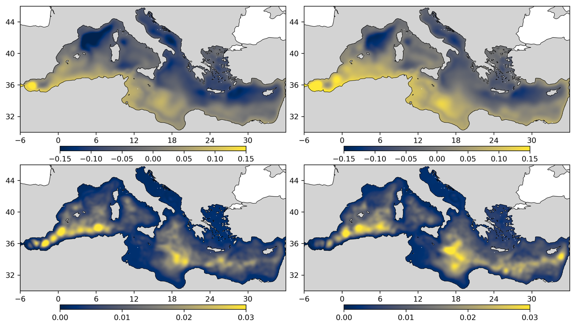
Figure 1 Prior ensemble mean (top panels) and standard deviation (bottom panels) for the low-frequency (interannual) component of sea surface height on January 1997 (left panels) and on January 2017 (right panels).

These ensemble data are nonetheless important to solve our estimation problem because they can be expected to contain useful information about the low-frequency variability of the sea, in particular through a non-stationary, non-homogeneous and anisotropic description of the correlation structure. Non-stationarity of the ensemble statistics comes as a result of the time-varying external forcing that is applied to the model.

3 Ensemble observational update

The purpose of this section is to describe the method that is applied to solve the estimation problem. We first formulate the problem in a Bayesian framework (Sect. 3.1). Then, we provide a description of the prior probability distribution (Sect. 3.2) and the observation constraint (Sect. 3.3). And finally, we present the iterative algorithm that is used to sample the posterior probability distribution (Sect. 3.4). In the following, the approach is described using a generic presentation. For our experiments, specific tuning and simplifications will be introduced as explained in Sect. 4.1.

3.1 Inverse problem

The vector of variables x that we want to estimate is going to include several components or subvectors x_i, which are presented here successively. Our first objective is to reconstruct the low-frequency variability of the Mediterranean, as described here by the dynamic topography H only (even if other variables could in principle be included):

$$\begin{array}{}\text{(1)}& {\mathit{x}}_{\mathrm{1}}=\left[H\right(x,y,t\left)\right].\end{array}$$

The spatial resolution of these fields (grid where x, y and z are discretized) is the same as the model ensemble simulation (i.e. 1/12° on the horizontal), and the time resolution (for t) is set to 1 month, which is sufficient to resolve the low-frequency component of the signal. These fields contain interannual time scales, without the annual cycle, which is filtered out.

In addition, since the estimation will use data from a prior ensemble model simulation, we must account for a possible bias in these data, which we also include in the vector of variables to estimate:

$$\begin{array}{}\text{(2)}& {\mathit{x}}_{\mathrm{2}}=\left[\mathit{\delta }H\right(x,y),\mathit{\delta }T(x,y,z),\mathit{\delta }S(x,y,z\left)\right].\end{array}$$

This bias is here assumed constant in time. A more complex problem would be to allow for a slow variation of this bias over time, and a simplification would be to rely on available climatologies to compute the bias beforehand as the difference with the model climatology, which would exclude the bias x₂ from the estimation vector. The complexity of the estimation problem needs to be tuned according to what is expected tractable with the available observations and methods.

Moreover, the estimation problem will require the covariance of the prior uncertainty and the covariance of the unresolved time scales (as the main contribution to the observation representativity error). Both can be obtained from the prior ensemble simulation, but again with possible biases (resulting for instance from an insufficient spread of the prior ensemble). This bias is introduced in the estimation vector, as two multiplicative factors applied to these two covariances:

$$\begin{array}{}\text{(3)}& {\mathit{x}}_{\mathrm{3}}=\left[\mathit{\alpha }\right(x,y),\mathit{\beta }(x,y\left)\right].\end{array}$$

These factors α and β are here assumed to be constant in time, but again more complex assumptions would be possible. The introduction of such amplification factors in the estimation vector is what is usually done in adaptive Kalman filters, as proposed for instance by Dee (1995), Hoang et al. (1998), Li et al. (2009), Mitchell and Houtekamer (2009) and applied by Brankart et al. (2010) to a square-root Kalman filter. It must be noted here that it may be challenging to estimate these two factors simultaneously, since it is always the sum of the prior and observation uncertainties that is observed. The joint estimate is still possible in principle (as in adaptive Kalman filters) if they have distinct correlation structures, but it is always possible that information is missing to obtain accurate estimates.

The vector of variables to estimate x is then built by aggregating the components (Eqs. 1–3): $\mathit{x}=[{\mathit{x}}_{\mathrm{1}},{\mathit{x}}_{\mathrm{2}},{\mathit{x}}_{\mathrm{3}}]$. It is estimated using the Bayes theorem:

$$\begin{array}{}\text{(4)}& p^a\left(\mathit{x}\right)=p\left(\mathit{x}|{\mathit{y}}^{\mathrm{o}}\right)\propto p^b\left(\mathit{x}\right)p\left({\mathit{y}}^{\mathrm{o}}|\mathit{x}\right)\end{array}$$

where y^o is the vector with all available observations, p^b(x) is the prior probability distribution for x, p(y|x) is the conditional probability distribution for the observation vector y given the state x of the system (evaluated at y=y^o to give the likelihood function of x), and p^a(x) is the posterior probability distribution for x, given the observations y^o. Our objective is to produce a sample of p^a(x).

The reason why we needed to include x₂ and x₃ in the estimation vector x is that the ensemble model simulation described in Sect. 2.2 could not be assumed perfectly reliable. We know that there are substantial biases and that the spread is not always sufficient to be consistent with the observations. By including x₂ and x₃, we provide more freedom in the prior statistics to fit the observations, and we expect to obtain a more reliable description of the posterior uncertainty, as described by p^a(x).

3.2 Prior probability distribution

The prior statistical model is meant to embed all assumptions that are made in this study. These are the assumptions that need to be checked and evaluated. Our central assumption is to use a long-term ensemble model simulation as a prior distribution for the low-frequency interannual signal. The expectation is that the model simulation embeds useful information about this signal, in particular through the use of a realistic interannual atmospheric forcing. The prior statistics are thus nonstationary, since they can change in time according to how the model responds to a changing atmosphere. There is also the perspective that they can improve in the future when the model is made more and more reliable.

The first consequence of this choice is that only a small-size ensemble is available (30 members), which means that we can only have a simple prior model (in our case, described by the mean and the covariance, with localization), since no complex model can be inferred from a small sample. The second consequence is that we have to cope with possible systematic errors in the model simulation (bias and insufficient spread), by including additional degrees of freedom in the estimation vector (x₂ and x₃).

In our model, the prior distribution for the components (Eqs. 2 and 3) of x (i.e. the bias and the spread adjustments) are assumed independent, while the distribution for x₁ (i.e. the main target of the inverse problem) depends on x₂ and x₃: $p^b\left(\mathit{x}\right)=p^b\left({\mathit{x}}_{\mathrm{1}}\right|{\mathit{x}}_{\mathrm{2}},{\mathit{x}}_{\mathrm{3}}\left)p^b\right({\mathit{x}}_{\mathrm{2}}\left)p^b\right({\mathit{x}}_{\mathrm{3}})$. We will see that this makes the resulting prior statistical model for x non-Gaussian, because the statistics of x₁ depends on x₂ and x₃, and because x₃ is itself assumed non-Gaussian.

For component 1, the conditional distribution (for given x₂ and x₃) is assumed Gaussian, with mean ${\mathit{x}}_{\mathrm{1}}^b$ and covariance ${\mathbf{P}}_{\mathrm{1}}^b$. ${\mathit{x}}_{\mathrm{1}}^b$ and ${\mathbf{P}}_{\mathrm{1}}^b$ are specified by the mean ${\mathit{x}}_{\mathrm{1}}^r$ and the covariance ${\mathbf{P}}_{\mathrm{1}}^r$ of the low-frequency component of the reference ensemble simulation (described in Sect. 2.2), with a bias correction given by x₂ and a spread correction given by the component α of x₃:

$$\begin{array}{}\text{(5)}& {\mathit{x}}_{\mathrm{1}}^b={\mathit{x}}_{\mathrm{1}}^r-{\mathit{x}}_{\mathrm{2}}\mathrm{and}{\mathbf{P}}_{\mathrm{1}}^b=\mathbf{D}\left(\mathit{\alpha }{)}^{\mathrm{1}/\mathrm{2}}{\mathbf{P}}_{\mathrm{1}}^r\mathbf{D}\right(\mathit{\alpha }{)}^{\mathrm{1}/\mathrm{2}}\end{array}$$

where D(α) is a diagonal matrix amplifying the variance of the reference ensemble simulation.

For component 2 (the bias estimate), the prior distribution is also assumed Gaussian, with zero mean and a covariance again obtained from the reference ensemble simulation:

$$\begin{array}{}\text{(6)}& {\mathit{x}}_{\mathrm{2}}^b=\mathrm{0}\mathrm{and}{\mathbf{P}}_{\mathrm{2}}^b={\mathbf{P}}_{\mathrm{2}}^r\end{array}$$

but this time, ${\mathbf{P}}_{\mathrm{2}}^r$ does not only include the interannual time scales, but also the annual cycle, which contains structures that can be expected in the model bias. The resulting prior variance is thus quite large to let the bias adjust almost freely to the observations.

For component 3 (the spread correction estimate), we assume a lognormal distribution, which is obtained as the exponential of Gaussian variables, with zero mean (${\mathit{x}}_{\mathrm{3}}^b=\mathrm{0}$) and an analytically specified covariance ${\mathbf{P}}_{\mathrm{3}}^b$. In ${\mathbf{P}}_{\mathrm{3}}^b$, the variance is set to be quite large, to let the spread of the distributions be expanded or reduced almost freely to fit the observations, and the correlation structure is specified by a Gaussian function of the distance: ${\mathit{\gamma }}_{\mathrm{3}}\left(r\right)=\exp (-r^{\mathrm{2}}/l_{\mathrm{3}}^{\mathrm{2}})$, where l₃=200 km. We need this length scale to be small enough to let α and β adjust to the observations, and large enough to avoid having too many degrees of freedom in the estimation vector (which would not be controllable by the observations).

In addition, since the covariance matrices of components 1 and 2 are provided by a small size ensemble (the 30 members of the ensemble simulation described in Sect. 2.2), they cannot be expected to represent adequately the correlation structure over the full Mediterranean basin and over the full time period (30 years). To cope with this difficulty, the classic approach (Houtekamer and Mitchell, 1998; Bishop and Hodyss, 2009) is to localize the ensemble covariance by a Schur product with a correlation matrix Γ_loc:

$$\begin{array}{}\text{(7)}& {\mathbf{P}}_i^{b,\mathrm{loc}}={\mathbf{P}}_i^b\circ {\mathbf{\Gamma }}_{\mathrm{loc}}\end{array}$$

where the correlation structure in Γ_loc is here specified by a Gaussian function of the distance r and time difference Δt:

$$\begin{array}{}\text{(8)}& {\mathit{\gamma }}_{\mathrm{loc}}(r,\mathrm{\Delta }t)=\exp \left(-r^{\mathrm{2}}/l_{\mathrm{loc}}^{\mathrm{2}}\right)\times \exp \left(-\mathrm{\Delta }{t}^{\mathrm{2}}/{\mathit{\tau }}_{\mathrm{loc}}^{\mathrm{2}}\right)\end{array}$$

with l_loc≃100 km and τ_loc≃6 months (tuned for our experiments). In this way, only the local ensemble correlation structure is used in the estimation problem, while the long-range ensemble correlations are dropped.

3.3 Observation constraint

Observation error is assumed Gaussian, with zero mean (unbiased observations) and covariance R. It is described by the probability distribution:

$$\begin{array}{}\text{(9)}& p\left(\mathit{y}\right|\mathit{x})={\displaystyle \frac{\mathrm{1}}{\sqrt{\left(\mathrm{2}\mathit{\pi }{)}^p\right|\mathbf{R}|}}}\exp \left[-{\displaystyle \frac{\mathrm{1}}{\mathrm{2}}}{\left(\mathit{y}-\mathbf{H}{\mathit{x}}_{\mathrm{1}}\right)}^T{\mathbf{R}}^{-\mathrm{1}}\left(\mathit{y}-\mathbf{H}{\mathit{x}}_{\mathrm{1}}\right)\right]\end{array}$$

where H is the observation operator, which is here only a linear interpolation from the component x₁ of the estimation vector (the only component that is directly observed) to obtain the observation equivalent (with dimension p). R is assumed diagonal and it is computed as the amplification of a reference error variance R^r by the factor β:

$$\begin{array}{}\text{(10)}& \mathbf{R}={\mathbf{D}}^{\mathrm{1}/\mathrm{2}}\left(\mathit{\beta }\right){\mathbf{R}}^{\mathrm{r}}{\mathbf{D}}^{\mathrm{1}/\mathrm{2}}\left(\mathit{\beta }\right)\end{array}$$

where D(β) is a diagonal matrix amplifying the variance R^r obtained from the reference ensemble simulation. It is here included in the estimation vector to adjust for a possible bias in the estimation of R^r.

The observation cost function is then:

$$\begin{array}{}\text{(11)}& \begin{array}{rl}{J}^{\mathrm{o}}\left(\mathit{x}\right)=& -\log p\left({\mathit{y}}^{\mathrm{o}}|\mathit{x}\right)={\displaystyle \frac{\mathrm{1}}{\mathrm{2}}}{\left({\mathit{y}}^{\mathrm{o}}-\mathbf{H}{\mathit{x}}_{\mathrm{1}}\right)}^T\\ & {\left[{\mathbf{D}}^{\mathrm{1}/\mathrm{2}}\left(\mathit{\beta }\right){\mathbf{R}}^{\mathrm{r}}{\mathbf{D}}^{\mathrm{1}/\mathrm{2}}\left(\mathit{\beta }\right)\right]}^{-\mathrm{1}}\left({\mathit{y}}^{\mathrm{o}}-\mathbf{H}{\mathit{x}}_{\mathrm{1}}\right)\\ & +{\displaystyle \frac{\mathrm{1}}{\mathrm{2}}}\sum _{j=\mathrm{1}}^p\log {\mathit{\beta }}_j+\mathrm{Cst}\end{array}\end{array}$$

where the last two terms result from the normalizing factor in Eq. (9), and β_j is the value of β corresponding to each observation [by interpolation of β(x,y)]. Since all matrices are diagonal, the computation of J^o can be written as a simple sum over all observations:

$$\begin{array}{}\text{(12)}& J^{\mathrm{o}}={\displaystyle \frac{\mathrm{1}}{\mathrm{2}}}\sum _{j=\mathrm{1}}^p\left[{\displaystyle \frac{{\left(y_j^{\mathrm{o}}-H_j{\mathit{x}}_{\mathrm{1}}\right)}^{\mathrm{2}}}{{\mathit{\beta }}_j{R}_j^r}}+\log {\mathit{\beta }}_j\right]\end{array}$$

which is straightforward to evaluate. The estimation of β thus results from a compromise between the two terms of Eq. (11), the first one decreasing with β and the second one increasing with β, and it is coupled to the estimation of the other components through x₁.

3.4 Iterative Monte Carlo method

In the above problem, none of the distributions p^b(x), p(y|x) or p^a(x) are Gaussian, or even approximately Gaussian, so that linear estimation methods are not directly applicable. In the following, we will show that Monte Carlo Markov Chains (MCMC) iterative sampling methods can be made efficient enough to solve this problem of large dimension.

The method is based on the Metropolis/Hastings algorithm (see e.g. Robert and Casella, 2004), which generates a sample of a target probability distribution [in our case, p^a(x)] by constructing a stochastic process (a Markov chain) that is in equilibrium with this target distribution. In other words, this means that we construct a stochastic process whose “attractor” is characterized by the distribution p^a(x) that we want to sample. In this algorithm, the next iterate of the Markov chain x_K+1 is computed from the current iterate x_K by sampling a perturbation of x_K from a simple proposal distribution (usually Gaussian) and then accepting or rejecting the perturbation according to the variation of the cost function. Perturbations decreasing the cost function are always accepted, while perturbations increasing the cost function are only sometimes accepted to ensure the equilibrium condition (see Appendix A1 for more details).

This algorithm is quite general and usually efficient enough as long as the number of dimensions is not too large (typically a few hundreds) because the cost of sampling a large-dimension proposal distribution, even if Gaussian, can be substantial. For instance, a classic choice for the proposal distribution would be to compute the proposal perturbation as a linear combination of EOFs (Empirical Orthogonal Functions), with random Gaussian coefficients, as done for instance in Gaultier et al. (2014) or Durán Moro et al. (2017). However, if the dimension of the state vector (n) is large and if there are many relevant directions of perturbations (m), the cost of this linear combination (n×m operations) becomes quickly prohibitive (up to n² for a perturbation with full rank covariance).

More specifically, in our practical example, even if we have only 30 members to define the prior probability distribution (which would make an acceptable value of m), we need to localize the prior covariance according to Eq. (7). This makes the prior covariance a full-rank matrix, and thus demultiply the number of possible directions of perturbations. Prior uncertainty really occurs in a large dimension space, which needs to be explored. This is what makes the computation of the random perturbation by a linear combination prohibitively expensive and impracticable for our large-size problem.

To cope with this difficulty, we can actually take advantage of the localization of the ensemble covariance by Eq. (7) using the method proposed and illustrated in Brankart (2019) and applied in Popov et al. (2024) to ocean colour observations. In this method, the random perturbation of the state vector is not computed as a linear combination of basis vectors, but by a Schur product of several vectors randomly taken from a pre-computed set of vectors. This Schur product is designed in such a way that the covariance of the random perturbation is given by Eq. (7).

Suppose for example that we have generated a sample of vectors ${\stackrel{\mathrm{̃}}{\mathit{x}}}_k^{\mathrm{loc}}$, k=1, …, m with covariance ${\stackrel{\mathrm{̃}}{\mathbf{\Gamma }}}_{\mathrm{loc}}$, where ${\stackrel{\mathrm{̃}}{\mathbf{\Gamma }}}_{\mathrm{loc}}$ is defined so that Γ_loc is the 6th Schur-power of ${\stackrel{\mathrm{̃}}{\mathbf{\Gamma }}}_{\mathrm{loc}}$. In practice, to be consistent with Eq. (8), this simply means that the correlation function corresponding to ${\stackrel{\mathrm{̃}}{\mathbf{\Gamma }}}_{\mathrm{loc}}$ must be:

$$\begin{array}{}\text{(13)}& {\stackrel{\mathrm{̃}}{\mathit{\gamma }}}_{\mathrm{loc}}\left(r\right)=\exp \left(-r^{\mathrm{2}}/\mathrm{6}{l}_{\mathrm{loc}}^{\mathrm{2}}\right)\times \exp \left(-\mathrm{\Delta }{t}^{\mathrm{2}}/\mathrm{6}{\mathit{\tau }}_{\mathrm{loc}}^{\mathrm{2}}\right)\end{array}$$

i.e. with a correlation length scale and a correlation time scale that are multiplied by $\sqrt{\mathrm{6}}$.

Then, we use the general property that the covariance of Schur product is the Schur product of the covariance: if we take 6 different vectors from the ${\stackrel{\mathrm{̃}}{\mathit{x}}}_k^{\mathrm{loc}}$, the covariance of their Schur product is the 6th Schur-power of ${\stackrel{\mathrm{̃}}{\mathbf{\Gamma }}}_{\mathrm{loc}}$, and thus Γ_loc. If we further make the Schur product of this vector by a vector obtained from the prior ensemble (with covariance ${\mathbf{P}}_i^b$), we obtain a pseudo-random perturbation vector with the localized covariance of Eq. (7), at the cost of just 6 Schur products (i.e. 6n operations). This last Schur product can be viewed as the modulation of one member of the ensemble simulation (more precisely the anomaly with respect to the ensemble mean) by one large-scale pattern with covariance Γ_loc, as more extensively explained in Brankart (2019) for the MCMC sampler, or in Bishop et al. (2017) in the framework of a localized ensemble Kalman filter.

The whole benefit comes from the fact that the sample ${\stackrel{\mathrm{̃}}{\mathit{x}}}_k^{\mathrm{loc}}$, k=1, …, m, with covariance ${\stackrel{\mathrm{̃}}{\mathbf{\Gamma }}}_{\mathrm{loc}}$ needs to be computed only once. Then, the diversity of the possible directions of perturbations will only result from the combinatorial effect of the Schur products. For instance, with m=30 and 6 Schur products, the number of different directions of perturbation is: $N=\mathrm{30}\times \mathrm{29}\times \mathrm{28}\times \mathrm{27}\times \mathrm{26}\times \mathrm{25}\times \mathrm{24}\simeq \mathrm{1.026}\times {\mathrm{10}}^{\mathrm{10}}$, which is sufficient to span all relevant degrees of freedom of our system. Actually, the effective number of degrees of freedom (d) depends on the ratio between the size of the domain (in space and time) and the localization scales, and it is very tiny as compared to N. The idea behind this large value of N is to produce a quasi-random sample of this target space of dimension d, and thus ideally among the largest possible number of directions of perturbation (which has here to be discrete because of the finite samples). See Brankart (2019) for more details. It must also be mentioned that the size of the localizing ensemble could also be larger than the size of the original ensemble, which would also increase N. We used here the same size for simplicity and to limit the memory requirements.

A full technical description of the algorithm used in this paper is provided in the Appendix, where a description of the computational complexity of the algorithm is also included. It is shown that the method can be very easily implemented to be efficient on GPUs, and that we were able to obtain a gain of about 100 as compared to CPUs in the computation of the solution of our problem.

4 Illustration of the ensemble results

By applying the method described in the previous section using the observation and model data presented in Sect. 2, we obtain an ensemble estimate of the low-frequency variability of the Mediterranean, i.e. a sample of the posterior distribution p^a(x). In this section, we provide a more precise description of the experiments that have been performed in terms of input data, specific settings and computational intensity (Sect. 4.1), we illustrate the results by a few statistics describing the solution (Sect. 4.2), we examine the importance of the model data to constrain the solution (Sect. 4.3), and we evaluate the reliability of the posterior ensemble (Sect. 4.4.)

4.1 Description of the experiments

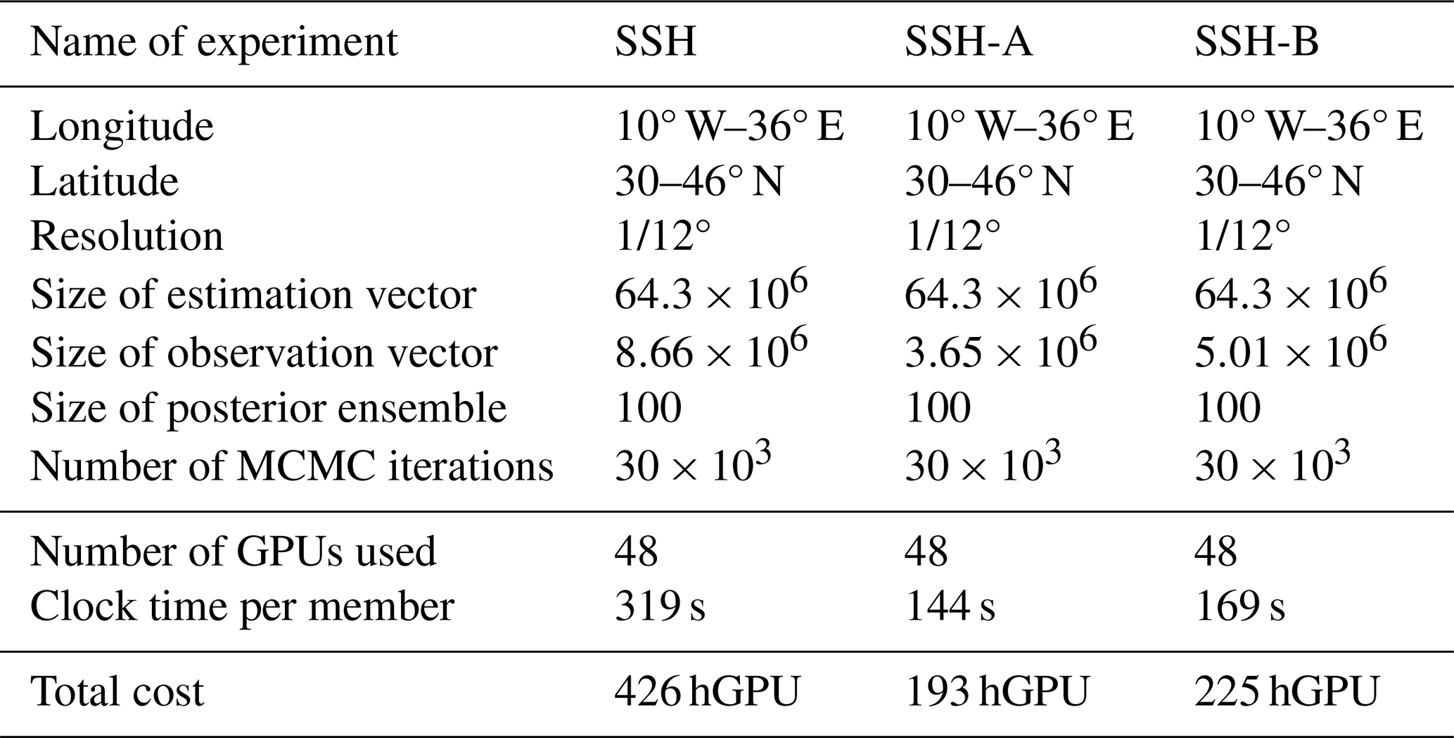
The first experiment (SSH) includes all available along-track altimetric observations. This experiment has been repeated twice (SSH-A and SSH-B) using the subsets of altimetric observations (A and B) described in Table 1. The characteristics of the experiments are given in Table 2.

Table 2 Characteristics of the experiments. Note that the total cost is to generate 100 ensemble members. One may not need so many members.

As compared to the method described in Sect. 3, one simplification has been introduced in the practical implementation: we preferred to rescale the prior standard deviation to a constant value (set to a typical value of 4 cm) rather than using the model ensemble standard deviation, because it is much too small in several regions (especially along the coast). This constant standard deviation is then adaptively rescaled by the free factor α (in the estimation vector). This simplification is here needed because it turned out that, in this problem, the estimation of α from the observations is not easy (see Sect. 5).

The cost of the experiments provided in Table 2 suggests that each member of the posterior ensemble can be obtained quite quickly and with moderate resources. It must be noted however that memory can also be a limitation in the size of the problem that can be afforded, because the whole prior ensemble must be in memory to keep the computation efficient. Since each GPU will load its share of the problem, a sufficient number of GPUs, each with enough memory, may thus be needed to solve a large-size problem.

4.2 A description of posterior uncertainty

As a first illustration of the solution of the problem, Fig. 2 shows the equivalent of Fig. 1 for the posterior ensemble of the SSH experiment, i.e. after the altimetric observation constraint has been applied. As an additional third line of panels, the figure also shows the corresponding low-frequency component of SSH obtained from the Aviso mapped (L4) dataset (but without a description of the associated uncertainty, see explanation at the end of this section). To obtain a comparable result, the same time filter as the one applied to the model data has been applied to the original Aviso maps to extract the low-frequency interannual signal only. From Fig. 2 (top panels), we can see that the posterior ensemble mean is substantially different from the ensemble mean of the model simulation (Fig. 1, top panels). A bias has been removed (see Sect. 5.1), and the detailed structure has also been reshaped by the observations. The ensemble mean has become very similar to the Aviso counterpart, despite being obtained very differently. In Aviso, all observable time scales are mapped first and the time filter is applied afterwards, while we here directly estimate the low-frequency component from the observations. We can thus conclude that the two approaches made a rather consistent use of the same along-track observations.

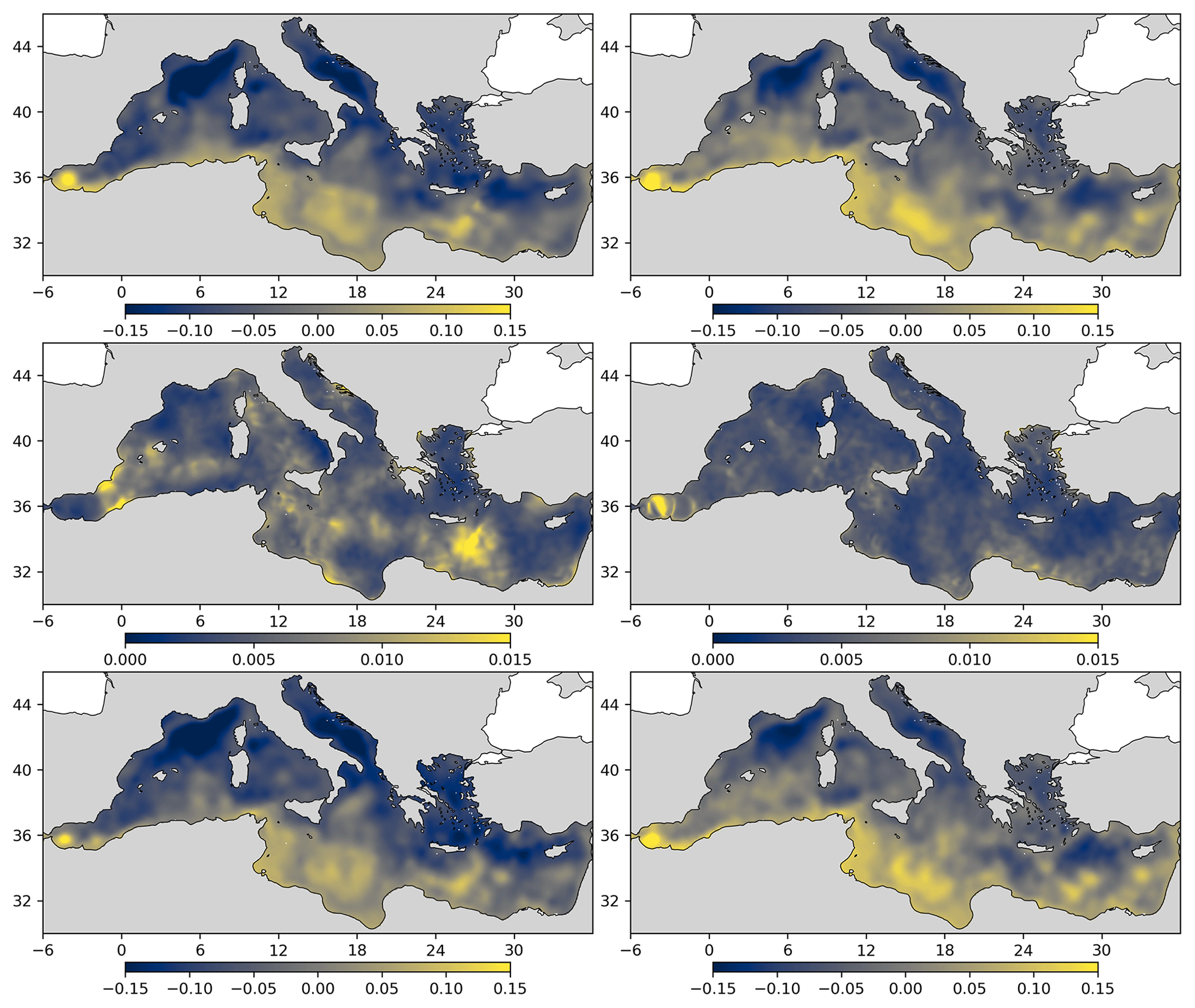
Figure 2 Posterior ensemble mean (top panels) and standard deviation (middle panels) for the low-frequency (interannual) component of sea surface height on January 1997 (left panels) and on January 2017 (right panels). This corresponds to the SSH experiment described in Table 2. The bottom panels show the corresponding low-frequency component of SSH obtained from the Aviso L4 product.

Regarding the spread of the ensemble (second line of panels in Figs. 1 and 2), we can see that it has been strongly reduced by the observation constraint. In 2017 (right panel), it is smaller than 1 cm in most of the Mediterranean (except in the Alboran Sea). At that date, there are indeed quite many altimetric satellites flying simultaneously, which provide enough data to mitigate uncertainty. The same figure for 1997 (left panel) displays more regions with higher values (up to 1.5 cm), especially in the gaps between the Topex/Poseidon ground tracks.

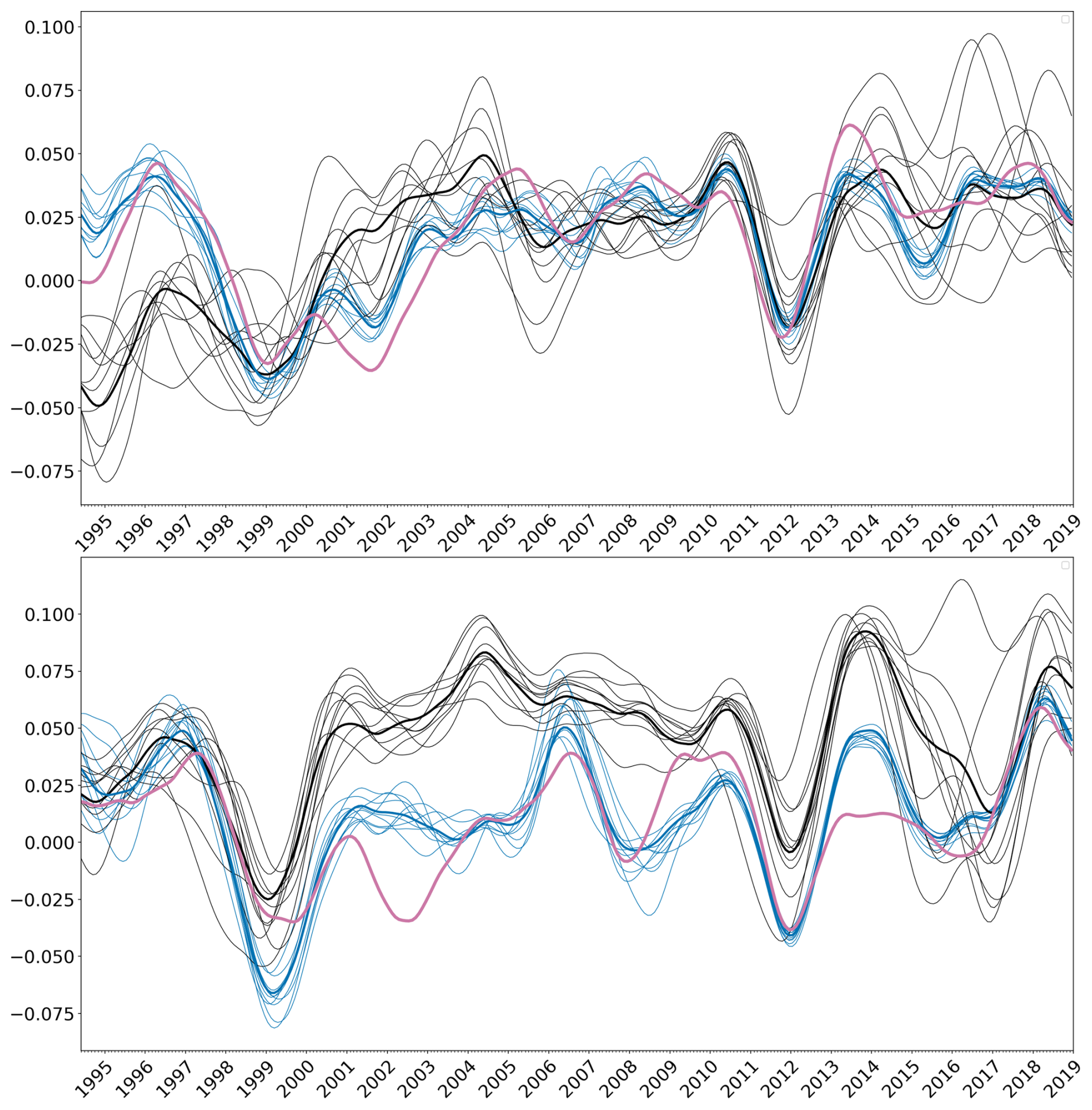
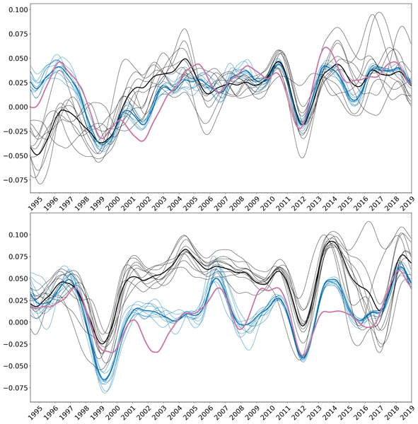
Figure 3 Low-frequency component of the sea surface height time series at 18.5° E, 35° N (top panel) and 17.1° E, 35° N (bottom panel). The figure compares the prior ensemble (black), the posterior ensemble (blue) and the Aviso L4 product (thick purple line). The black and blue thick lines are the corresponding ensemble means.

To illustrate the time variation of this residual uncertainty, Fig. 3 shows time series of a subset of 10 ensemble members for the prior ensemble (in black) and for the posterior ensemble (in blue). The ensemble means are represented as thicker lines, and the Aviso counterpart is in purple. This is shown at two close locations in the Ionian Sea: one at the points of high density in Topex/Poseidon and ERS ground tracks (18.5° E, 35° N), and the other one (17.1° E, 35° N) in a gap where the uncertainty is large in the early years of the altimetric measurements. In this figure, we can see the correction of the bias and the reduction of the spread in the updated ensemble as compared to the model ensemble. The updated ensemble also becomes more consistent with the Aviso time series, even if, in such local time series, there can be differences, which are mostly due to the smallest scales. At the Topex/Poseidon crossover location, the spread of the ensemble stays small over the full period, while at the gap location, the spread is larger at the beginning of the period and decreases with time as more satellite observations become available.

It must also be noted that, by producing an ensemble solution, we keep track of the residual uncertainty occuring at all scales (and, more generally, on any derived quantity). For instance, if one is interested in larger spatial scales, it is still possible to apply a smoothing operator on the ensemble members and see how the ensemble spread, and thus uncertainty, is decreased. Actually, in our solution, much of the spread displayed in Figs. 2 and 3 (and the misfit with Aviso) is due to the smallest scales being imperfectly observed. By contrast, in the current version of the Avsio mapped product, the residual uncertainty is not described by an ensemble, but by a map of the error standard deviation. From this information only, it is impossible to deduce the uncertainty on derived quantities, like the low-frequency component of the signal, which is why it could not be displayed in our figures.

4.3 Importance of the prior model simulation

In the MCMC method, the ensemble model simulation provides the local space and time correlation structure of the succesive random perturbations that are summed up to obtain every member of the updated ensemble. It is thus playing a central role in filling the gaps between observations, especially if they are sparse (in space and time), and in shaping the spread of the updated ensemble. It can vary in space and time according to the model dynamical behaviour. Length scales and time scales are not always and everywhere the same. Anisotropy can be forced by the presence of dynamical structures, like currents, or by topography, in particular along the coastline. Figure 4 illustrates the prior correlation structure for sea surface height with respect to two specific locations in the Mediterranean (9.65° E 37.45° N and 12.43° E 38.00° N) in January 2006. This corresponds to the model correlation structure, as obtained specifically for the low-frequency component of the signal, and with localization, using Eq. (7).

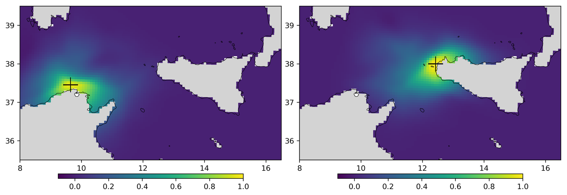
Figure 4 Prior correlation structure with respect to sea surface height at two specific locations in the Mediterranean: 9.65° E 37.45° N (left panel) and 12.43° E 38.00° N (right panel).

In this figure, we can observe that the field decorrelates across strong currents or across coastlines, and the importance of localization to drop unreliable long-range correlations. It can also be asymmetric in time, which means that depending on where and when we are, future and past observations can have a different weight in the solution. Our assumption in this paper is that, at least for the low-frequency component of the signal, this information is best obtained by an interannual ensemble model simulation spanning the same period as the observations, with the perspective that it can be progressively improved, following future model enhancements.

4.4 Reliability of the solution

A classic approach to assess the reliability of the ensemble solution is to build a rank histogram using independent observations (Anderson, 1996). In our case, we can check the ensemble from experiment SSH-A using observations from subset B, and we can check the ensemble from experiment SSH-B using observations from subset A (see the definition of the subsets in Table 1). To make the comparison with observations, we need to compute the ensemble equivalent to each individual observation, perturb the ensemble members by a random noise with the statistics of the observation error, and compute the rank of the observation in the resulting ensemble of values (sorted in ascending order). If the independent observation is consistent with the ensemble solution, then the probability distribution of the rank must be uniform. A necessary condition of reliability is thus that the rank histogram is flat.

Figure 5 (top panels) shows the rank histogram obtained for SSH-A and SSH-B. As compared to the observations, we can see that the ensemble solution is globally unbiased and only slightly overdispersive. The two bumps in the external regions of the histogram indicates that the detailed shape of the probability distribution is not perfectly consistent with the observations, with a bit too much probability both in the central regions and towards the extreme values. It must be noted however that what is checked here is the sum of posterior uncertainty and observation error, and that the amplitude of observation errors was also part of the estimation problem. It is thus for instance possible to obtain a flat histogram with underestimated posterior uncertainty and overestimated observation error. These two probability distributions cannot be verified separately using independent observations only.

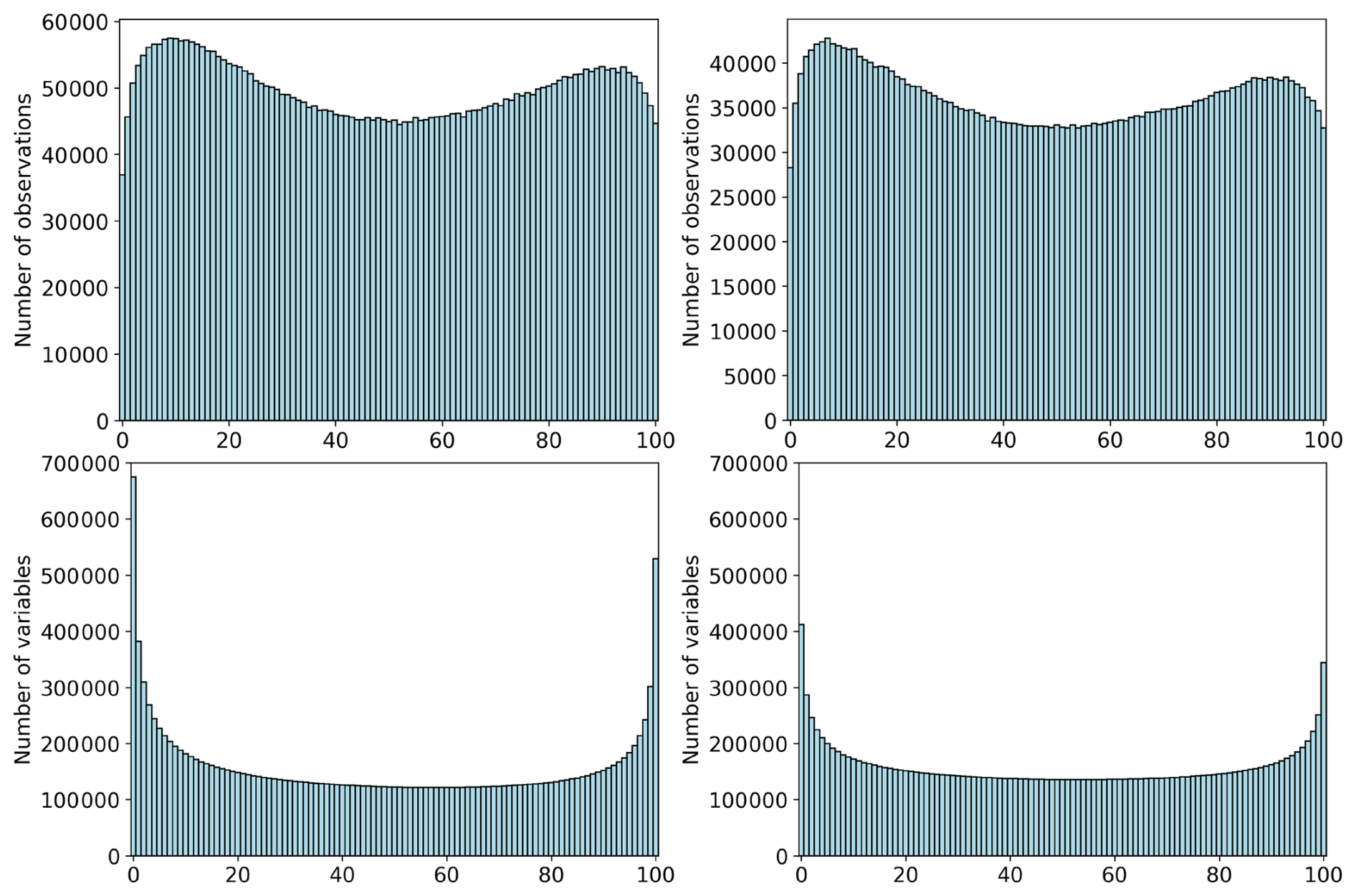
Figure 5 Rank histogram of independent observations in updated ensemble (top panels), as obtained using observations of subset B to check experiment SSH-A (top left panel), and observations of subset A to check experiment SSH-B (top right panel). Rank histogram of members of the SSH updated ensemble (i.e. using all observations) in the updated ensembles using partial observations (bottom panels), i.e. using members of experiment SSH to check experiment SSH-A (bottom left panel) and experiment SSH-B (bottom right panel).

To further check the consistency of the ensemble solution, we can compare experiment SSH (using all observations) to experiment SSH-A and SSH-B. Experiment SSH can indeed be viewed as the posterior ensemble obtained by conditioning the ensemble SSH-A to the observations of subset B or the ensemble SSH-B to observations of subset A. It should thus be consistent with the two of them. Figure 5 (bottom panels) shows the rank histogram of members of the ensemble SSH (at all grid points) in the ensemble obtained with experiment SSH-A (left panel) and experiment SSH-B (right panel). The result is averaged over members so that the numbers correspond to number of grid points in one member. What we can see is that the ensembles SSH-A and SSH-B are slightly underdispersive to be consistent with the ensemble SSH, which suggests that the spread (i.e. the posterior uncertainty) is presumably a bit too small in all posterior ensembles. This can directly result from oversimplified statistical assumptions, which may give too much confidence in the observations, for instance by assuming uncorrelated observation errors.

5 Adaptive estimation of statistical parameters

In the inverse problem described in Sect. 3, statistical parameters were also included in the estimation vector to cope with systematic errors in the prior statistics of the model simulation and with the imperfect knowledge of the observation errors (mainly representativity errors). In the following, we describe the resulting ensemble estimates for the simulation bias (Sect. 5.1), for the missing simulation variance (Sect. 5.2), and for the observation error variance (Sect. 5.3). These results are illustrated for the SSH experiment only.

5.1 Identification of the simulation bias

The first byproduct of the estimation procedure is an ensemble estimate of the bias in the prior ensemble simulation, as here directly obtained from the along-track altimetric observations. Figure 6 shows the ensemble mean (left panel) and standard deviation (right panel) of this bias estimate. In the ensemble mean, the most salient features are a too weak cyclonic circulation in the Balearic Sea and the South-Western Algerian basin (yellow anomaly), and too weak Iera-Petra and Pelops gyres in the Eastern basin (blue anomaly), as already mentioned in Héron et al. (2026).

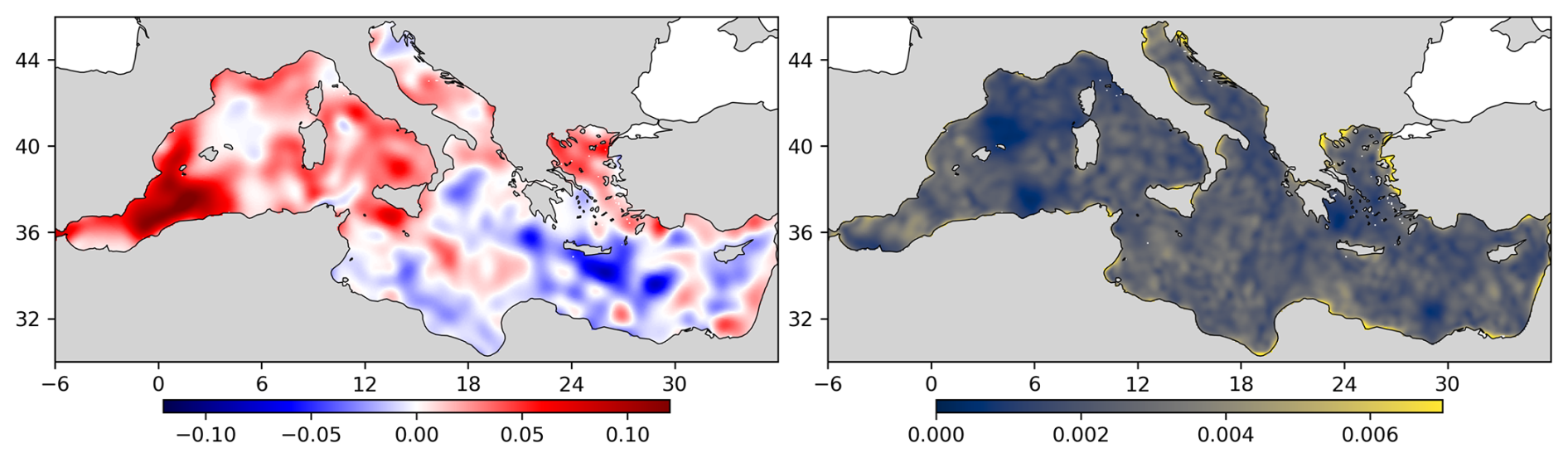
Figure 6 Posterior 100-member ensemble estimate of the bias: ensemble mean (left panel) and standard deviation (right panel).

On the other hand, from the ensemble standard deviation, we can see that the uncertainty on the bias is quite small over the whole domain. This means that all Markov chains have converged towards a very similar map of the bias parameter to ensure best compatibility with observations (despite a zero-mean prior distribution for the bias, and with a large associated uncertainty). The largest residual uncertainty on the bias (Fig. 6, right panel) is along the coast (particularly in the Adriatic and Aegean seas), where the observation constraint is weaker.

5.2 Estimate of the missing simulation variance

Our experiments also embed an adaptive estimate of the prior ensemble standard deviation (through the correcting factor α in component x₃). Figure 7 (top left panel) shows that the best estimate obtained with the MCMC procedure is always between 3 and 5 cm (i.e. quite close to the prior value of 4 cm). More precisely, what the figure shows is the corrected value of the standard deviation by an estimated factor computed as the exponential of the ensemble mean of the log of α (since the factor α was assumed lognormal).

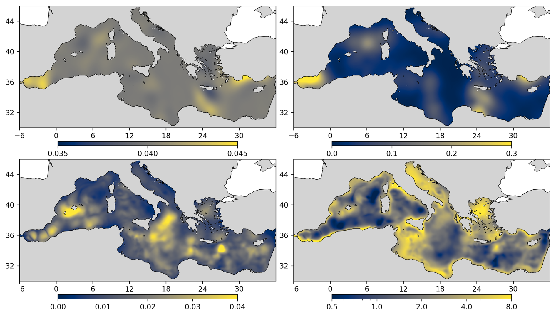
Figure 7 Estimate of the standard deviation of the prior uncertainty (top left panel) and estimated relative error (top right panel), as obtained from the MCMC estimation procedure. As a complement, the bottom left panel show a more direct estimate of the standard deviation of the prior uncertainty, as obtained from the difference between the prior and posterior ensembles, while the bottom right panel displays the ratio between this estimate and the prior ensemble standard deviation.

On the other hand, the top right panel of Fig. 7 shows the standard deviation of the log of α, which gives an idea of the relative error on the estimate, thus here typically between 5 % and 30 %. This could look like an acceptable estimation, but actually, from this figure and from the variety of patterns displayed by the ensemble members, we must conclude that we were not able to provide an accurate adaptive estimate of the prior variance with this method. The various Markov chains just spread from their background value, without converging towards a common pattern, as it happens when a parameter is not controllable by the observations. This is why we had to start from a constant prior (4 cm) and use a moderate prior standard deviation for α (30 %) to keep the prior distribution within reasonable bounds.

As a more direct diagnostic of what the standard deviation of the prior ensemble should have been to be compatible with the observations, we can compute the standard deviation of the misfit between the prior and posterior ensembles (after the bias correction has been applied). The result is shown in Fig. 7 (bottom left panel), which confirms that the estimate obtained from the observations as a byproduct of the MCMC sampler (top left panel) is not reliable. The standard deviation of this misfit between prior and posterior ensembles (bottom left panel) can be compared to the actual spread of the prior ensemble displayed in Fig. 1 (bottom panels). The ratio between these two maps (i.e. the ratio between the required spread and the actual spread) is also displayed in Fig. 7 (bottom right panel). It is a kind of time average that is computed as the square root of the ratio between the time-averaged variances. This ratio informs us about the amount of missing uncertainties in the ensemble simulation to be compatible with the real world, and can thus serve as a guideline to track the regions where variance is missing in the model world.

From the figure, we can see that the prior ensemble simulation has enough variance in the deep basins (the ratio is about 1) where the intrinsic variability can be viewed as dominant. At some places (with a ratio lower than 1), it is even too large to be compatible with the observations. However, in many other regions, especially along the coasts and in shallow basins, the model largely underestimates its own uncertainty (the ratio is much larger than 1). In this case, improving the model reliability would require simulating explicitly the missing sources of uncertainty in the model, such as for instance uncertainties in the atmospheric forcing, at the boundaries (Gibraltar Strait, runoffs), or the effect of the unresolved scales.

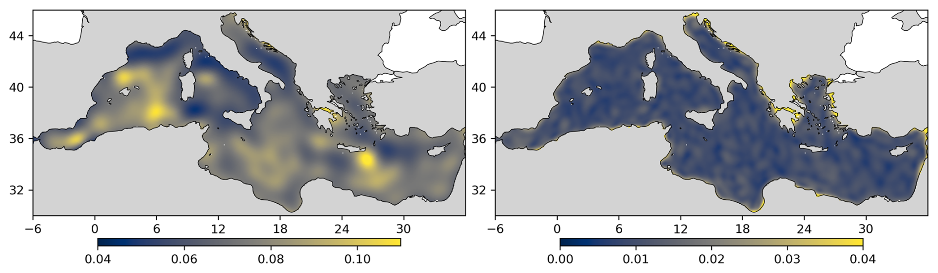
Figure 8 Estimate of the observation error standard deviation (left panel) and estimated relative error (right panel), as obtained from the MCMC estimation procedure.

5.3 Estimate of the observation error variance

The prior probability distribution that we used for the observation error standard deviation (σ₀) is a lognormal distribution with the mean and standard deviation both set to 5 cm. This means that we assumed a large prior uncertainty on the statistics of observation errors, which leaves much freedom to adjust it as part of the estimation vector (factor β in component x₃). This was useful in our system because observation errors not only contains the measurement error, but also all unresolved scales. In our case, this includes all high-frequency scales up to the annual cycle, so that the tuning of σ₀ would have required information about the residual signal (which we excluded from our estimation problem). One possibility is then to assume that it is almost unknown and adjust σ₀ as part of the estimation process.

Figure 8 illustrates the resulting estimate of σ₀. The left panel displays the ensemble mean (actually using the exponential of the ensemble mean of the log of β), which shows that the estimated standard deviation of the unresolved scales is larger in the regions of intense mesoscale activity, for instance where eddies detach from the Algerian current or at the location of the Iera-Petra and Pelops gyres. This is where the misfit between the observations and the low-frequency signal that we estimate is the largest.

On the other hand, the right panel of Fig. 8 shows that the relative error on this estimate is low everywhere (about 1 % in most of the domain, and up to 4 % along the coast), which means that all Markov chains converge to about the same map for σ₀. Moreover, we can verify that σ₀ automatically adjusts so that the value of the observation cost function (the first term of Eq. 12) becomes close to $p/\mathrm{2}$ (where p is the number of observations), which is the expected value that it must have when the system is optimal (Talagrand, 1999).

6 Conclusions

In this paper, a method has been proposed to estimate directly the low-frequency component of the ocean variability from native observations (along-track altimetry). The method provides an ensemble description of the solution, so that uncertainties can be properly assessed using independent data. Auxiliary statistical parameters (like the prior bias) can also be included in the estimation vector to enhance the description of prior uncertainties or observation uncertainties. The method is based on an MCMC sampler (modified to include a time and space localization of the prior covariance), which is shown efficient enough to solve large size problems, and which is well suited to work with MPI and GPUs. In our application, the main limitation was the memory required to store the prior ensemble on the GPUs.

The method was applied to reconstruct the interannual variability of sea surface height on the whole Mediterranean basin over a 26-year period (1993–2018). The result of the experiment was assessed against independent observations (by cross-validation), showing good reliability (flat rank histogram), even if self-consistency checks suggest a possible underestimation of uncertainties. Regarding the estimation of the auxiliary statistical parameters, the method produces a consistent estimate of the model bias and of the observation error variance (mainly representativity error in most places), but shows more difficulties in estimating the missing prior variance. In the latter case, the additional statistical parameter (α) is left almost free and thus only increase the prior variance without much control by the observations.

The diagnostic of this kind of experiment should provide insights on what is missing in the prior model simulation (in terms of variance and covariance) to be compatible with observations. To produce reliable ensemble reanalyses, forecasts or projections, it is indeed important that the main sources of modelling uncertainties are adequately represented. This would be especially important in multivariate applications, where a good description of the covariances between variables is needed. In our experiment, the model intrinsic variability is clearly insufficient to explain the whole misfit between simulation and observations. A better statistical agreement would require the explicit simulation of additional sources of uncertainty, for instance by moving towards a stochastic formulation of the model, as proposed for instance by Brankart et al. (2015) for the NEMO model, and recently developed in the CROCO model. Such an evolution of the model towards a more realistic description of uncertainties would not only be useful to improve the solution of modelling and estimation problems, but also to understand which observations are most needed to provide the missing information (for instance, through observation system simulation experiments).

Appendix A: Description of the algorithm

The purpose of this appendix is to provide more details on the algorithm that has been used to perform the ensemble observational update. It is based on the MCMC sampler proposed by Brankart (2019), as a variant of the Metropolis/Hastings algorithm (as described for instance in Robert and Casella, 2004). The presentation is here simplified to what is actually used in this paper, without all mathematical justifications and further possibilities.

A1 The Monte Carlo Markov Chain

As in the Metropolis/Hastings algorithm, each iteration of the Markov chains (x_K, K=1, …, N) proceeds in two steps:

1. Draw a candidate x^′ for the next iterate from a proposal probability distribution: ${\mathit{x}}^{\prime }\sim \mathit{\pi }\left({\mathit{x}}^{\prime }\right|{\mathit{x}}_K)$, which can be viewed as a random perturbation from x_K. This distribution must be easy to sample, as for instance a Gaussian distribution centered on x_K.

2. Accept the candidate x^′ as next iterate x_K+1 with probability:

   $$\begin{array}{}\text{(A1)}& q=\min \left({\displaystyle \frac{p^a\left({\mathit{x}}^{\prime }\right)}{p^a\left({\mathit{x}}_K\right)}}{\displaystyle \frac{\mathit{\pi }\left({\mathit{x}}^{\prime }|{\mathit{x}}_K\right)}{\mathit{\pi }\left({\mathit{x}}_K|{\mathit{x}}^{\prime }\right)}},\mathrm{1}\right)\end{array}$$

   which is simplified to $q=\min \left(p^a\right({\mathit{x}}^{\prime })/p^a({\mathit{x}}_K),\mathrm{1})$ if the proposal distribution is symmetric [$\mathit{\pi }\left({\mathit{x}}^{\prime }\right|{\mathit{x}}_K)=\mathit{\pi }({\mathit{x}}_K\left|{\mathit{x}}^{\prime }\right)$], as for instance for a Gaussian distribution centered on x_K. In this symmetric case, the acceptance probability means that the candidate x^′ is always accepted if the cost function decreases [$p^a\left({\mathit{x}}^{\prime }\right)>p^a\left({\mathit{x}}_K\right)$], and only sometimes accepted if the cost function increases [$p^a\left({\mathit{x}}^{\prime }\right)<p^a\left({\mathit{x}}_K\right)$].

This Markov chain statisfies the condition of local equilibrium with p^a(x), which means that if x_K is distributed as p^a(x), then x_K+1 is also distributed as p^a(x). At equilibrium, the probability of being at x_K and move from x_K to x_K+1 is equal to the probability of being at x_K+1 and move from x_K+1 to x_K. With very few restrictions on p^a(x) and on the proposal distribution (as long as regular), this Markov chain will converge towards sampling p^a(x).

In our implementation, both step 1 and step 2 are slightly different from the original Metropolis/Hastings algorithm, by exploiting the additional assumptions that (i) the prior probability distribution of the observational update is based on Gaussian distributions, (ii) it is described by a moderate size ensemble, and (iii) the ensemble covariance is localized by a Schur product with a parameterized correlation matrix Γ_loc.

In step 1, the sampling of the proposal distribution is defined by:

$$\begin{array}{}\text{(A2)}& {\mathit{x}}^{\prime }=\sqrt{{\displaystyle \frac{K}{K+\mathrm{1}}}}{\mathit{x}}_K+\sqrt{{\displaystyle \frac{\mathrm{1}}{K+\mathrm{1}}}}\mathit{\xi }{\mathit{x}}_{\mathit{\pi }}\end{array}$$

where ξ is a Gaussian random number with zero mean and unit standard deviation [$\mathit{\xi }\sim \mathcal{N}(\mathrm{0},\mathrm{1})$], and x_π is a pseudo-random direction of perturbation, whose covariance is the covariance of the localized prior ensemble. In all equations, all state vectors are always assumed to be zero mean anomalies, which means that the prior ensemble mean has been substracted before running the algorithm.

To generate x_π efficiently, we assume that Γ_loc is the sth Schur-power of another correlation matrix ${\stackrel{\mathrm{̃}}{\mathbf{\Gamma }}}_{\mathrm{loc}}$, and that we have previously generated a moderate size sample of ${\stackrel{\mathrm{̃}}{\mathbf{\Gamma }}}_{\mathrm{loc}}$: ${\stackrel{\mathrm{̃}}{\mathit{x}}}_k^{\mathrm{loc}}$, k=1, …, m. A pseudo-random direction of perturbation x_π can then be computed as the Schur product:

$$\begin{array}{}\text{(A3)}& {\mathit{x}}_{\mathit{\pi }}={\mathit{x}}_j^b\circ {\mathit{x}}_{i_{\mathrm{1}}}^{\mathrm{loc}}\circ {\mathit{x}}_{i_{\mathrm{2}}}^{\mathrm{loc}}\circ \mathrm{\dots }\circ {\mathit{x}}_{i_s}^{\mathrm{loc}}\end{array}$$

where ${\mathit{x}}_j^b$ is one random member of the prior ensemble (anomaly with respect to the mean) and i₁, …, i_s are random indices from the sample ${\stackrel{\mathrm{̃}}{\mathit{x}}}_k^{\mathrm{loc}}$, k=1, …, m. In our application, we have set m=30 and s=6. From Eq. (A3), it follows that x_π has the same covariance as the localized ensemble (P^b∘Γ_loc), since the covariance of the Schur product of vectors is the Schur product of their covariance. This method provides an efficient way to compute pseudo-random directions of perturbation in large dimension. At the cost of only s Schur products, we sample from a set of $P=m\mathrm{!}/(m-s-\mathrm{1})\mathrm{!}$ possibilities, which makes $P=\mathrm{30}\times \mathrm{29}\times \mathrm{28}\times \mathrm{\dots }\times \mathrm{24}\simeq \mathrm{1.026}\times {\mathrm{10}}^{\mathrm{10}}$ possibilities with our particular settings.

Without step 2 (i.e. if all candidates x^′ are accepted), the iteration of Eq. (A2), starting from a zero initial condition (x₀=0), is going to provide a sample of the prior probability distribution, i.e. with the same covariance as the prior ensemble with localization. As a side usage, this can be useful to resample the prior ensemble for various purposes. This means that the prior distribution is already accounted for in step 1, and that the acceptance probability q in step 2 must only account for the variation of the likelihood function:

$$\begin{array}{}\text{(A4)}& \begin{array}{rl}q& =\min \left[{\displaystyle \frac{p\left({\mathit{y}}^{\mathrm{o}}\right|{\mathit{x}}^{\prime })}{p\left({\mathit{y}}^{\mathrm{o}}|{\mathit{x}}_K\right)}},\mathrm{1}\right],\mathrm{with}{\displaystyle \frac{p\left({\mathit{y}}^{\mathrm{o}}|{\mathit{x}}^{\prime }\right)}{p\left({\mathit{y}}^{\mathrm{o}}|{\mathit{x}}_K\right)}}\\ & =\exp \left[J^{\mathrm{o}}\left({\mathit{x}}_K\right)-J^{\mathrm{o}}\left({\mathit{x}}^{\prime }\right)\right]\end{array}\end{array}$$

which only requires the computation of the observation cost function J^o for the candidate iterate x^′. In the case of Gaussian observation errors with diagonal covariance, this reduces to:

$$\begin{array}{}\text{(A5)}& J^{\mathrm{o}}={\displaystyle \frac{\mathrm{1}}{\mathrm{2}}}\sum _{j=\mathrm{1}}^p{\displaystyle \frac{\mathrm{1}}{R_j}}{\left(y_j^{\mathrm{o}}-y_j^{\prime }\right)}^{\mathrm{2}}\end{array}$$

where $y_j^{\mathrm{o}}$, j=1, …, p are the observations, R_j, the associated error variance, and $y_j^{\prime }=H_j{\mathit{x}}^{\prime }$, where H_j is the observation operator associated to observation j. However, with a linear H_j, the normal implementation of the algorithm is to augment x with y=Hx in all inputs, so that y^′ is already available as part of x^′ to evaluate J^o. In this case, the only operations performed in the running of the ensemble of Markov chains are given by Eqs. (A2)–(A5), together with the small task of sampling ξ in Eq. (A2), and sampling the indices j, i₁, …, i_s in Eq. (A3). It must also be noted that in the case of adaptive observation error variances, the observation cost function is slightly more complicated, as explained in Sect. 3.3 (see Eq. 12).

A2 Computational complexity

With this algorithm, a separate Markov chain must be simulated to sample each member of the posterior ensemble. The overall cost C is thus proportional to the size m^′ of the posterior ensemble (which may be smaller or larger than the size m of the prior ensemble) and to the number N of iterations required by the Markov chains. For each posterior ensemble member, the cost of each iteration depends on the size n of the vector to estimate x, the size p of the observation vector, the number s of Schur products, and the average number ν of candidates x^′ needed before the next iterate is accepted. Considering that, until the candidate x^′ is accepted, Eqs. (A2) and (A3) need only be applied to the observed part of the vectors, the cost of each iteration is as follows: (νp+n) operations for Eq. (A2), s(νp+n) operations for Eq. (A3), and νp operations for Eq. (A5). The overall cost C of the algorithm is thus:

$$\begin{array}{}\text{(A6)}& C\sim m^{\prime }N\left[\right(s+\mathrm{1}\left)\right(\mathit{\nu }p+n)+\mathit{\nu }p]=m^{\prime }N\left[\right(s+\mathrm{2})\mathit{\nu }p+(s+\mathrm{1}\left)n\right].\end{array}$$

The cost is linear in n and p, the factor s applies to most of the cost, and the factor ν only applies to the part of the cost that is proportional to p.

Regarding the cost, the main difficulty with this algorithm is that the number of iterations required to reach convergence is difficult to anticipate. As discussed in more details in Brankart (2019), we can however compare the cost with other algorithms by computing the number of iterations N_eq that could be afforded to obtain an equivalent cost. For instance, if we compare with a classic implementation of the Ensemble Kalman Filter (EnKF Evensen, 2003), which is also compatible with the localization of the ensemble covariance by a local-support correlation matrix, this number of iteration would be (Brankart, 2019):

$$\begin{array}{}\text{(A7)}& N_{\mathrm{eq}}\sim {\displaystyle \frac{d{\mathit{\rho }}^{\mathrm{2}}}{\mathit{\nu }m}}\end{array}$$

where m is the size of the updated ensemble (here always the same as the size of the prior ensemble), d is the average number of local observational update in which each observation is used, and ρ is the root mean square number of observation used in each local observational update. For instance, in our problem, typical values would be at least (if there is one local update per horizontal grid point and per monthly timestep): νm∼10², d∼10⁵, ρ∼10⁴, and thus N_eq∼10⁷. In our particular application, the cost of the classic implementation of the EnKF would thus have been substantially larger (because the number and density of observation is large, and because the cost of each local update in the EnKF is proportional to the cube of the number of observations). Moreover, the MCMC sampler offers a set of possibilities that is different from the EnKF, such as the adaptive mechanism used in this paper, which makes it relevant for a different set of applications (with possible overlaps).

A3 Efficiency with MPI and with GPUs

The simplicity of the algorithm, as described by Eqs. (A2) to (A5), makes it straightforward to obtain efficient implementations with MPI and with GPUs.

On the one hand, with MPI, each processor need only take care of one segment of the estimation vector and one segment of the observation vector (which do not need to be related to each other and without overlap between processors). The only data that need to be communicated between processors are: (i) the factor ξ in Eq. (A2), (ii) the random indices j, i₁, …, i_s in Eq. (A3), and (iii) the resulting cost function J^o in Eq. (A5), which must be summed over all processors. MPI parallelization thus comes very easily with very little extra cost.

On the other hand, all operations in Eqs. (A2), (A3) and (A5) are vector operations so that they can be easily distributed on the GPU (in our case, in Fortran, with OpenACC instructions). To be efficient, this requires that the size of the estimation vector and the size of the observation vector on each processor are large enough (typically n>10⁴ and p>10⁴) to keep all components of the GPU busy. Moreover, this computation requires that the prior ensemble and the observation vector be transfered to the memory of the GPU (more precisely the segment used by the current processor if MPI is also applied). This transfer of data takes non-negligible time if it is done at each iteration of the Markov chain (because the numerical cost of just one iteration is comparatively too small). Explicit instructions must be given (in our case through OpenACC requests) to perform this transfer of data only once before the first iteration. This cost then becomes negligible as the number of iterations increases (typically for N>10³). With these conditions on the size of the problem and on the number of iterations, we were able to accelerate the computation by a factor of about 100 as compared to the performance obtained when the GPU accelerators are not activated.