Topographic control of tides in the Ross Sea: eddy-like structures, bottom-trapped waves, and energetics

Using a regional high-resolution coupled ocean-sea ice-ice shelf model, this study investigates tide-topography interactions, energy conversions, and tide-induced cross-slope exchange in the Ross Sea. The model resolves tidal time series and power spectral density that agree well with available mooring data. Through tidal decomposition of modelled tides, we identify a diurnal topographic mode along the Ross Sea slope, characterized by three eddy-like structures. These structures arise because the varying topography of the continental slope induces divergence and convergence in the diurnal surface-mode tidal flows. This generates sea surface height extremes that persist longer than the time required for geostrophic adjustment, allowing rotating geostrophic flows (i.e., the topographic mode) to develop around them. The topographic mode dominates the water exchange across the slope and yields a net heat transport towards the shelf (∼12 TW). The surface and topographic modes can exchange energy with each other, as indicated by alternating positive and negative patches of energy conversion rate with a magnitude reaching 1 W m⁻². The baroclinic tides in the Ross Sea manifest as bottom-trapped waves over the continental slope and other topographic gradients. The energy of baroclinic tides, primarily converted from the topographic mode, is an order of magnitude smaller than the barotropic tides. The barotropic component accounts for most of the tidal dissipation along the slope (∼0.1 W m⁻²), with a minimal contribution from baroclinic tides. This study identifies tides as an important driver of heat transport onto the Antarctic shelf, which is fundamental for accurate prediction of future Antarctic ice shelf melt and global sea level rise.

1 Introduction

Around Antarctica, tides are a fundamental driver of ocean dynamics. They accelerate the Antarctic Slope Current and contribute to the formation of the Antarctic Slope Front through convergence along the continental slope (Flexas et al., 2015; Stewart et al., 2019). Tides also modulate ice–ocean stress (Si et al., 2022) and drive cross-shelf overturning circulation (Garreau and Maze, 1992; Pérenne et al., 2000; Stewart et al., 2019). Beneath ice shelves, tidal sea-level fluctuations exert direct stress on the ice base, inducing flexure and promoting iceberg calving (Riedel et al., 1999; Legrésy et al., 2004; Fricker and Padman, 2006). Tidal currents further influence the dynamics of ice streams that feed ice shelves (Doake et al., 2002; Legrésy et al., 2004; Brunt et al., 2010). In addition, tides enhance vertical mixing and turbulence, facilitating upward heat flux and thereby increasing basal melting beneath ice shelves (MacAyeal, 1984a; Holland and Jenkins, 1999; Robertson, 2013; Liu et al., 2023).

Antarctic Bottom Water (AABW), a key component of the global thermohaline circulation (Orsi et al., 1999; Jacobs, 2004), is formed through processes significantly influenced by tides. Tidal currents mix precursor water masses, such as Circumpolar Deep Water (CDW), Antarctic Surface Water (AASW), and Dense Shelf Water (DSW), at the continental shelf break, with mixing intensity modulated by tidal phase, topography, and stratification (Whitworth and Orsi, 2006; Padman et al., 2009). Beyond mixing, tides also facilitate cross-slope exchange of these water masses (Gordon et al., 2004; Ou et al., 2009; Padman et al., 2009; Castagno et al., 2017; Stewart et al., 2018). By suppressing entrainment in DSW overflows, tides promote the formation of colder and denser AABW (Ou et al., 2009; Guan et al., 2009; Han et al., 2024).

As a primary source of AABW, the Ross Sea exhibits complex tidal dynamics. Research on tides in the Ross Sea began in the early 20th century with ship-based measurements (Darwin, 2009). Following the International Geophysical Year (post-1957), tidal observations intensified, culminating in the first synthesized studies (Gilmour et al., 1962). Successive studies using a gravity station network on the Ross ice shelf (Williams and Robinson, 1980) and moored current meters near and on the ice shelf (Pillsbury and Jacobs, 1985) identified both diurnal and semi-diurnal constituents, with the diurnal tides being dominant. Subsequent instrument deployments, such as moorings (Gordon et al., 2004; Whitworth and Orsi, 2006), CTDs (Castagno et al., 2017), and GPS stations (Brunt et al., 2010) yielded data that facilitated enhanced analysis of tides in the Ross Sea. Satellite altimetry addressed the sparseness of in situ data, revealing ice shelf flexure in response to oceanic tides (Fricker and Padman, 2006) and enabling the extraction of accurate tidal signals (Ray, 2008). These altimeter data have also been used to develop sophisticated tidal models through data assimilation (Padman et al., 2003, 2018). Given that conducting in situ measurements poses significant logistical challenges, numerical models were developed to simulate tides (MacAyeal, 1984b; Padman et al., 2003; Robertson et al., 2003) and to assess their influence on physical processes such as thermohaline circulation (MacAyeal, 1984a; Padman et al., 2009; Wang et al., 2010) in the Ross Sea.

Previous works have documented general characteristics of the tides in the Ross Sea. Padman et al. (2003) first mapped barotropic tidal currents and sea surface height (SSH), providing a two-dimensional framework that Robertson et al. (2003) and Robertson (2005) extended through three-dimensional modelling, characterizing baroclinic tides and their role in mixing. However, these studies did not separate topographically controlled wave modes, such as vorticity waves (Padman et al., 2003) and continental shelf waves (Robertson, 2005), from the underlying tidal Kelvin wave (Robertson, 2005). Such separation is essential for understanding how topography modulates tidal flow. Moreover, while Robertson (2005) identified semi-diurnal constituents as the primary source of baroclinic tides, the studies of D'Asaro and Morison (1992) and Falahat and Nycander (2015) indicate that diurnal tides can also generate internal tides poleward of their critical latitude (∼30°), typically as bottom-trapped waves. At present, the generation, distribution, and role of such bottom-trapped waves in the Ross Sea remain unexplored. Moreover, existing estimates of tidal energy (Müller, 2013; Falahat and Nycander, 2015) rely on global models that may not adequately represent localized bathymetric effects. A comprehensive tidal energy budget analysis specifically focused on the Ross Sea is therefore needed.

This study employs a high-resolution numerical model, combined with tidal decomposition and energy diagnostics, to investigate tide-topography interactions, their associated energy conversions, and their implications for cross-slope exchange in the Ross Sea. The paper is organized as follows: Sect. 2 describes the numerical model and outlines the procedures for tidal analysis. Section 3 presents tidal characteristics and provides a comprehensive analysis of both tidal dynamics and energetics. Finally, the findings are summarized and discussed in Sect. 4.

2 Methods

2.1 Model Description

This study utilizes the Ross Sea regional ocean–sea ice–ice shelf coupled model (ROSIM_v5km), developed and validated by Yan et al. (2023), to examine tides in the Ross Sea. The model is based on the Massachusetts Institute of Technology's general circulation model (MITgcm; Marshall et al., 1997), which solves the hydrostatic Navier-Stokes equations on an orthogonal curvilinear grid under the Boussinesq approximation. It incorporates a dynamic-thermodynamic sea ice model (Zhang and Hibler, 1997; Zhang and Rothrock, 2000) and a thermodynamic ice shelf model (Losch et al., 2010).

The model domain, ranging between 86.5–60.6° S and 116.9° E–105.9° W, encompasses the Ross Sea with ice shelves and the surrounding open ocean (Fig. 1). The computational grid features a quasi-uniform horizontal resolution of 5 km (420×520 grid points) and 70 vertical layers, with layer thickness increasing from 10 m at the surface to 600 m at the bottom. The model topography is constructed from the Refined Topography Data Set 2 (Schaffer and Timmermann, 2016) and is represented using a partial cell scheme to minimize artificial flow distortion from stair-step topography approximations. Lateral boundary conditions for ocean and sea ice fields are prescribed at the northern, eastern, and western open boundaries of the model domain. For the ocean, the prescribed velocity, temperature, and salinity are extracted from the monthly mean climatology of the Southern Ocean State Estimate (SOSE; Mazloff et al., 2010; Verdy and Mazloff, 2017) 2005 to 2010 solution (iteration 100). Tidal currents applied at the open boundaries are obtained from the Circum-Antarctic Tidal Simulation version 2008 (CATS2008; Howard et al., 2019), which incorporates 10 major tidal constituents (M_f, M_m, K₂, S₂, M₂, N₂, K₁, P₁, O₁, and Q₁). Sea ice boundary conditions, including ice thickness, concentration, velocity, and snow thickness, are obtained from SOSE and the National Snow and Ice Data Center (Fetterer et al., 2017). Atmospheric forcing (10 m wind speed, 2 m temperature, 2 m dewpoint temperature, total precipitation, and mean surface downward radiation flux) is derived from the European Centre for Medium-Range Weather Forecasts Reanalysis v5 dataset (ERA5; Hersbach et al., 2023), which offers global meteorological fields with a spatial resolution of 0.25° and temporal resolution of an hour. The details regarding the model configuration and parametrizations have been described by Yan et al. (2023). The model was integrated from 1979 to 2019, with hourly outputs of 2003–2004 saved for analyzing tidal dynamics, as this period coincides with available mooring observations (introduced later in Sect. 2.2) and enables direct model–observation comparison.

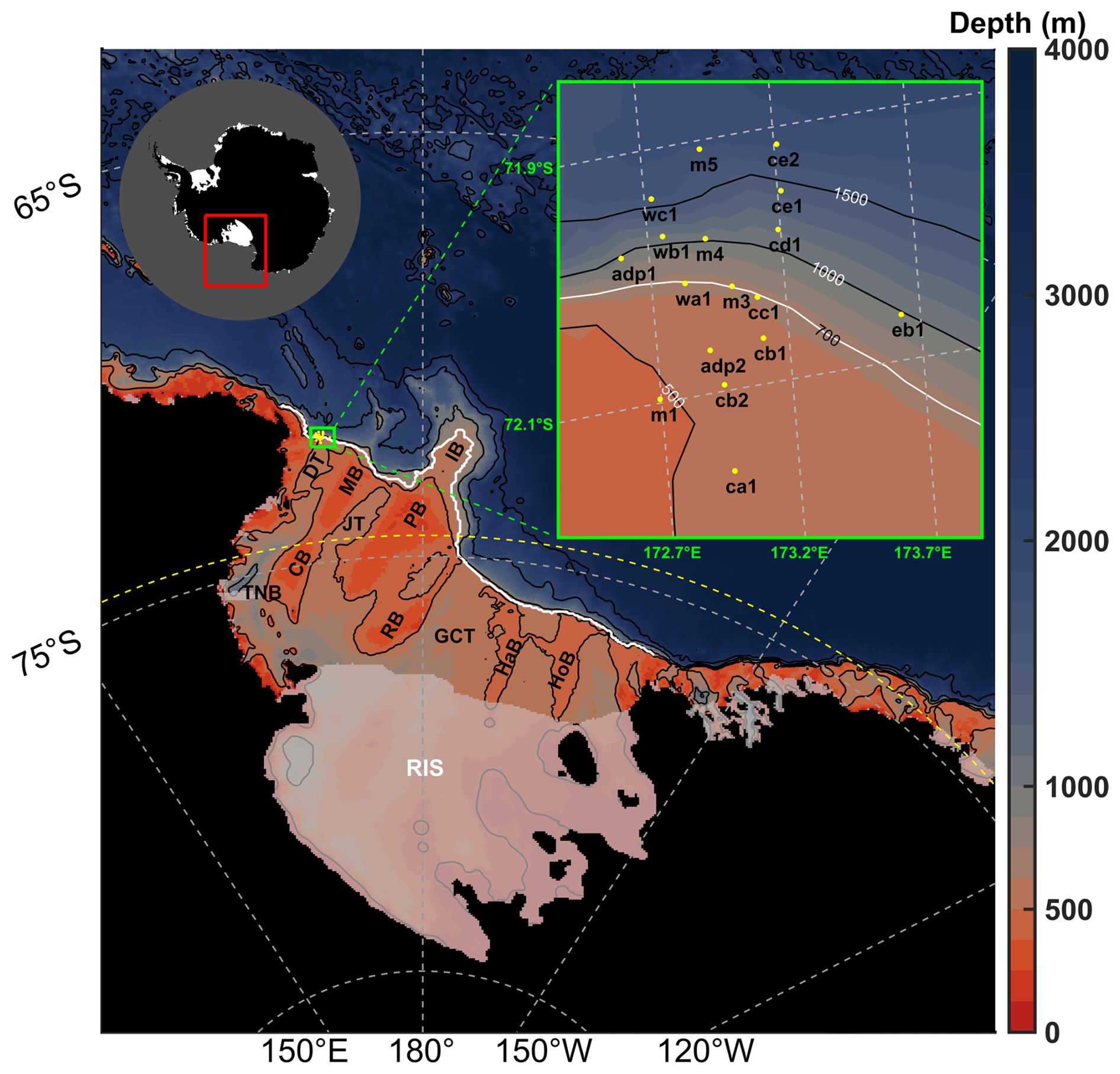
Figure 1 Map of the bathymetry within the model domain (outlined by the red box in the inset). Topographic features are depicted with color shading, and the ice shelves are rendered semi-transparent (DT: Drygalski Trough; JT: Joides Trough; GCT: Glomar Challenger Trough; IB: Iselin Bank; CB: Crary Bank; MB: Mawson Bank; PB: Pennell Bank; RB: Ross Bank; TNB: Terra Nova Bay; HaB: Hayes Bank; HoB: Houtz Bank). The yellow dashed line marks the latitude of 74.5° S (semi-diurnal critical latitude mentioned in Sect. 3.3). The yellow dots indicate the hydrographic mooring stations from the Antarctic Slope (AnSlope) program, outlined by the green inset box. Bathymetric contours (black lines) are drawn for the 500, 1000, 2000, and 3000 m depths. The white line marks the selected segment of the 700 m isobath on the slope, which is used for subsequent analysis.

2.2 Model Validation

The model's performance in simulating key components, such as sea ice production, water mass properties, and ice shelf melting, was validated by Yan et al. (2023), and its simulation of circulation over the continental shelf and slope was validated by Liu et al. (2025). In this study, we validate the simulated tides in the Ross Sea, by both benchmarking them against previous model studies, and comparing with hydrographic timeseries observations.

2.2.1 Observational data and processing

For model validation of tidal simulations, this study uses velocity observations from the AnSlope (Cross-slope exchanges at the Antarctic Slope Front) project. The dataset comprises Acoustic Doppler Current Profiler (ADCP) and Rotor Current Meters (RCM) records from 17 mooring stations deployed at the mouth of DT (yellow dots in Fig. 1), spanning multiple periods from March 2003 to March 2004 (for more details, see Table 1 in Gordon et al., 2009).

Mooring motion can contaminate velocity measurements (Kalvaitis, 1974; Langlois and Maze, 1990; Harding et al., 2017). During the AnSlope project, strong currents exerted considerable drag on the mooring lines, causing significant blow-down (Padman et al., 2009) and compromising some of the collected data (Gordon et al., 2009). To mitigate this, we only use data measured by the deepest ADCP or RCM at each station, as such instrument is closest to the anchor, where line tension is greatest, and thus experiences the least vertical and horizontal displacement (Susanto and Gordon, 2005). Our validation adopts a point-to-point comparison, matching the deepest observed point to the horizontally nearest model grid cell, then selecting the nearest valid cell within that column. While this introduces minor spatial mismatches, the dominant barotropic tidal scales far exceed grid spacing, making horizontal offsets of a few kilometers negligible. Furthermore, local baroclinic tides are bottom-trapped, non-propagating waves that affect amplitude but not the barotropic phase. Thus, a single depth suffices. Semi-diurnal and diurnal tidal constituents are extracted using the t_tide harmonic analysis package (Pawlowicz et al., 2002) for both observations and model output.

The interaction of tidal currents with sloping topography can generate a rectified mean flow (Garreau and Maze, 1992; Chen and Beardsley, 1995; Pérenne et al., 2000); therefore, comparing observed and simulated mean currents provides indirect validation of the tidal simulation. However, the mean flow varies strongly with height within the bottom boundary layer, and in steep areas, the model's bottom depth is likely not the same as the actual one, making the same absolute depth incomparable between the model and observations. This issue is compounded by mooring blow-down, which introduces time-dependent instrument depths and complicates fixed-depth assessments. To address this, we select several deep observation points at each station, specifically those least affected by mooring motion, and vertically average their time-mean velocities to define the observed mean flow. The corresponding model mean flow is derived by applying the same vertical and temporal averaging over the equivalent depth range and time period at the nearest grid cell. This procedure reduces sensitivity to vertical mismatches between observed and modelled depths.

2.2.2 Validation results

For comparison with previous studies, we calculated the two key diagnostic parameters defined by Padman et al. (2002, 2003): the root-sum-square of tidal harmonic amplitude and the time-averaged tidal flow speed. The spatial patterns shown in our Fig. 2 are consistent with those presented in Fig. 2 of Padman et al. (2003), whose results were derived from both “forward” (dynamical) and “inverse” (data assimilation) models.

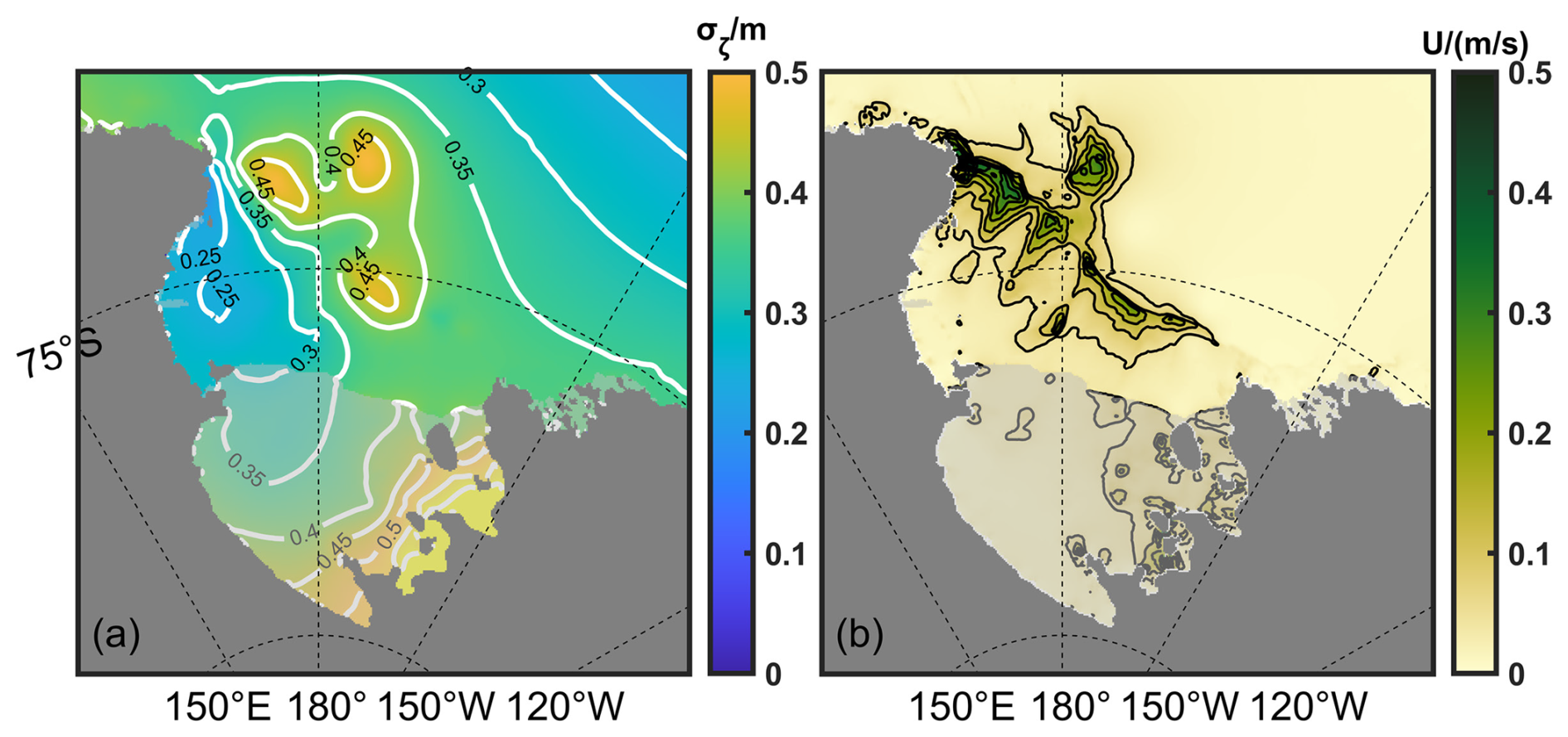
Figure 2 Spatial patterns of tidal characteristics calculated by definitions from Padman et al. (2002, 2003): (a) Root-sum-square of tidal harmonic amplitude ${\mathit{\sigma }}_{\mathit{\varsigma }}=\sqrt{\sum a_i}$ (m), where a_i is the amplitude of the ith tidal harmonic and (b) Time-averaged tidal flow speed (m s⁻¹).

The model's performance in simulating tides is further validated by comparing the time series and power spectral density (PSD) of tidal currents between the model output and observational data. For brevity, only the comparison for central mooring station cc1 is presented in the main text (Fig. 3); the results for the remaining 16 moorings are shown in the Supplement (Figs. S1–S16). Notably, a mismatch is found at station adp1 (Fig. S1), where the observed stronger semi-diurnal signal likely stems from the advective effects of the diurnal tides (Bell, 1975), as the slope there may exceed the resolving capability of the model's vertical grid.

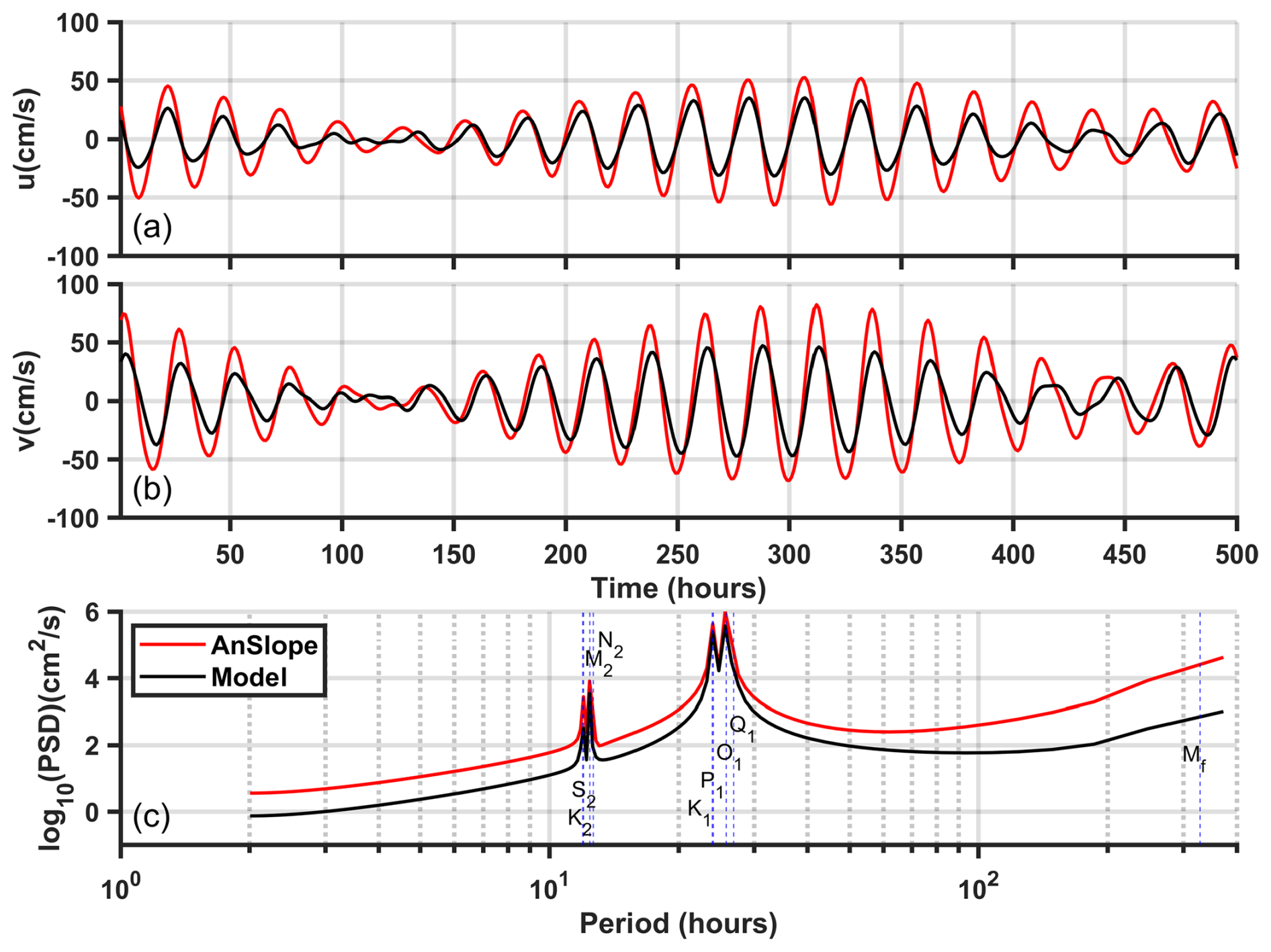
Figure 3 A comparison of the simulated and observed tidal currents at mooring station cc1 (for details, see Table S1 in the Supplement), showing the filtered time series (semi-diurnal and diurnal constituents) of the (a) meridional and (b) zonal tidal velocities, and (c) the corresponding power spectral density (PSD). The blue dashed lines indicate the periods of the corresponding tidal constituents (labelled adjacent to the lines). Simulated and observed data are shown in black and red, respectively.

As shown in Fig. 3c, the simulated tidal current energy shows peaks at diurnal and semi-diurnal frequencies matching the observations, although its magnitude is somewhat underestimated (especially for the M_f constituent). The good agreement between model and observations in the filtered time series (Fig. 3a and b) validates that the model correctly captures the phase of the predominantly diurnal current, and also reproduces the spring-neap cycle well. This lends credibility to studying the tidal dynamics and energetics in the Ross Sea using the model output.

The comparison between simulated and observed mean currents is presented for 13 mooring stations (Fig. 4). Although current velocity observations are available from 17 stations, some are located close enough to map to the same horizontal model grid cell. For each such group, only the station with the closest match between observed and modelled seafloor depth was retained. The model agrees well with observations at most stations, capturing the mean flow in both magnitude and direction, though a few individual stations exhibit discrepancies. It should be noted that the observed mean flow likely reflects the background Antarctic Slope Current rather than purely tidally rectified flow. Nevertheless, the overall consistency demonstrates the model's ability to reproduce the mean circulation, thereby lending indirect support to the reliability of the tidal simulation. Additionally, we compare the modelled cross-slope temperature section with observations from the PRISM project (Fig. S17 in the Supplement). The model reproduces cross-slope thermal structure, revealing the extension of CDW from the deep ocean onto the continental shelf. This provides further independent validation of the model's representation of water-mass properties. Overall, these results reinforce confidence in our subsequent estimate of tidally driven cross-slope heat transport.

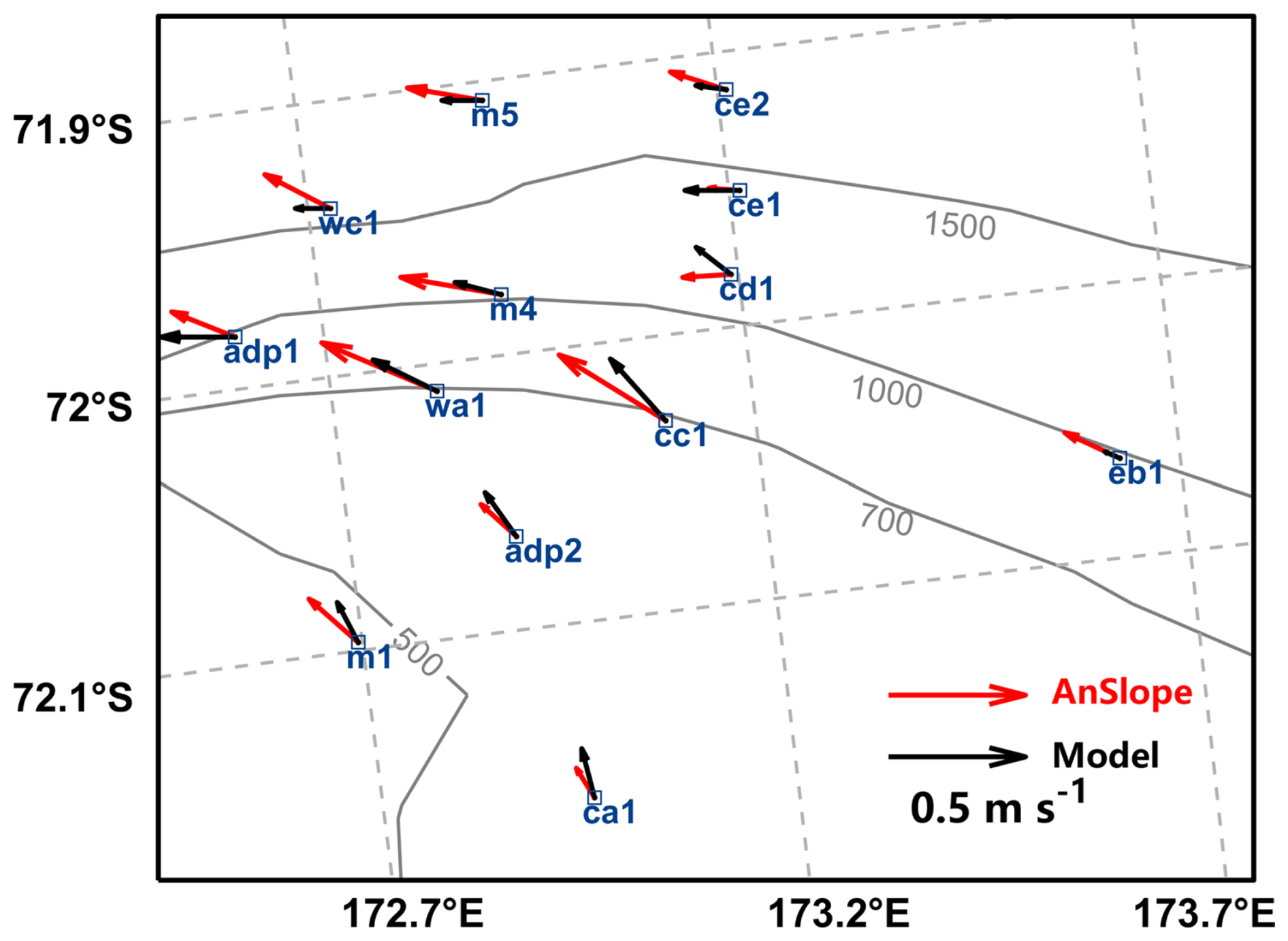
Figure 4 Comparison of the observed (AnSlope project) and simulated depth-averaged mean currents on the slope. Simulated and observed data are shown in black and red, respectively. Bathymetric contours (grey lines) are drawn for the 500, 700, 1000, and 1500 m depths. Mooring locations are indicated by open blue squares.

2.3 Extraction of tidal signals

The diversity of oceanic motions in the Ross Sea, which extends beyond tidal signals, necessitates harmonic analysis. However, the computational resources required for the analysis at all model grids are substantial. Combining the Fourier transform and dynamic analysis based on the vorticity equation, Wang et al. (2023) developed an efficient approach to extract wavy motions from full flow. Notably, in regions where the latitude is higher than the critical latitude of the tidal constituent, the wavy motions extracted by their method represent pure tidal signals, whereas at latitudes below the critical latitude, the extracted signals contain not only tidal components but also other wavy features. Since part of the Ross Sea lies below the critical latitude for semi-diurnal tides (∼74.5° S, shown by yellow dashed line in Fig. 1), a tidal filter following Wang et al. (2023) is used to extract tidal signals:

$$\begin{array}{}\text{(1)}& \begin{array}{rl}{M}_{\text{tide}}& (k,l,\mathit{\omega })=\\ & \left\{\begin{array}{ll}\mathrm{0},& \text{if }\mathit{\omega }\ne n\cdot {\mathit{\omega }}_{\text{tide}}\text{ at }(k,l,\mathit{\omega })\\ \mathrm{1},& \text{if }\mathit{\omega }=n\cdot {\mathit{\omega }}_{\text{tide}}\text{ at }(k,l,\mathit{\omega })\end{array}\right.(n=\mathrm{1},\mathrm{2}),\end{array}\end{array}$$

where k and l denote wavenumbers in the x- and y-directions, and ω_tide denotes the frequency of any tidal constituent.

For any physical variable A from the model outputs, the tidal signals can be derived by applying a forward Fourier transform, multiplying the result by a filter function, and subsequently performing an inverse Fourier transform:

$$\begin{array}{}\text{(2)}& A_{\text{tide}}=F^{-\mathrm{1}}\left(F\right(A)\times M_{\text{tide}}),\end{array}$$

where F denotes Fourier-transform, F⁻¹ the inverse Fourier-transform, and × the multiplication. The extracted signals include both the fundamental tidal constituent (n=1) and its first harmonic (n=2), which is generated by the advective effects of the barotropic tide (Bell, 1975). In this study, the method of Wang et al. (2023) is applied to extract tidal components of both velocity and density perturbations.

2.4 Modal Decomposition of Barotropic Tides

The barotropic tide can be divided into two parts, referred to as the surface mode and the topographic mode, following the framework of Tanaka (2023):

$$\begin{array}{}\text{(3)}& {\displaystyle }\begin{array}{rl}{\displaystyle \frac{\mathrm{1}}{H}}{\mathrm{\nabla }}^{\mathrm{2}}{\mathit{\psi }}_{\mathrm{S}}+\mathrm{\nabla }{\displaystyle \frac{\mathrm{1}}{H}}\cdot \mathrm{\nabla }{\mathit{\psi }}_{\mathrm{S}}& +J\left({\displaystyle \frac{\mathrm{1}}{H}},\mathit{\varphi }\right)=\mathrm{0},\\ & {\mathit{\psi }}_{\mathrm{S}}=\mathit{\psi }\text{at boundaries},\end{array}\text{(4)}& {\displaystyle }{\mathit{\psi }}_{\mathrm{T}}=\mathit{\psi }-{\mathit{\psi }}_{\mathrm{S}},\text{(5)}& {\displaystyle }{\mathit{u}}_{\mathrm{S}}={\displaystyle \frac{\mathrm{1}}{H}}(\mathrm{\nabla }\mathit{\varphi }+\mathit{k}\times \mathrm{\nabla }{\mathit{\psi }}_{\mathrm{S}}),\text{(6)}& {\displaystyle }{\mathit{u}}_{\mathrm{T}}={\displaystyle \frac{\mathrm{1}}{H}}(\mathit{k}\times \mathrm{\nabla }{\mathit{\psi }}_{\mathrm{T}}),\text{(7)}& {\displaystyle }{C}_{\mathrm{S}\to \mathrm{T}}={\mathit{\rho }}_{\mathrm{0}}{\mathit{\psi }}_{\mathrm{T}}\left[{\displaystyle \frac{f}{H}}{\mathrm{\nabla }}^{\mathrm{2}}\mathit{\varphi }+\mathrm{\nabla }{\displaystyle \frac{f}{H}}\cdot \mathrm{\nabla }\mathit{\varphi }-J\left({\displaystyle \frac{\mathrm{1}}{H}},{\mathit{\psi }}_{\mathrm{S}}\right)\right],\end{array}$$

where ψ and ϕ are potential and stream functions derived from the Helmholtz decomposition of the depth-integrated transport field, and H is the thickness of water column. $J(a,b)=\frac{\partial a}{\partial x}\frac{\partial b}{\partial y}-\frac{\partial b}{\partial x}\frac{\partial a}{\partial y}$ denotes the Jacobian operator. u_S and u_T are velocity fields associated with the surface and topographic modes, respectively. C_S→T is the energy conversion rate from the surface to the topographic mode.

This decomposition method rests on two key assumptions: (i) SSH variations are entirely attributable to the surface mode (Eq. 5), and (ii) the topographic mode solely accounts for the relative vorticity (Eq. 6). Physically, the surface mode corresponds to Kelvin waves, as illustrated by Tanaka (2023). The topographic mode has been attributed to topographic Rossby waves by Tanaka (2023) because topographic Rossby waves are eigenmodes of a continuously stratified coastal ocean with a sloping bottom and a coastal boundary (Wang and Mooers, 1976). Note, however, the continental slope in the Ross Sea is too steep to favor their generation (Han et al., 2023, 2024). In our model, the decomposition does yield a topographic mode, but it does not behave as a propagating Rossby wave (further discussed in Sect. 3).

2.5 Energetics analysis

In addition to the barotropic tides, we explore the generation of baroclinic tides and provide a comparative analysis of the energetics associated with both barotropic and baroclinic tidal motions. The barotropic velocity U and baroclinic velocity u^′ are defined as

$$\begin{array}{}\text{(8)}& {\displaystyle }\mathit{U}=(U,V,\mathrm{0})={\displaystyle \frac{\mathrm{1}}{H}}\stackrel{\mathrm{‾}}{{\mathit{u}}_H},\text{(9)}& {\displaystyle }{\mathit{u}}^{\prime }=(u^{\prime },v^{\prime },w)=\mathit{u}-\mathit{U}=(u-U,v-V,w),\end{array}$$

where ${\mathit{u}}_H=(u,v)$, $\mathit{u}=(u,v,w)$, with u, v and w being the zonal, meridional, and vertical tidal velocities, respectively. SSH is denoted by η, the bottom depth by h, and the total water depth by $H=\mathit{\eta }+h$. The notation $\stackrel{\mathrm{‾}}{(*)}={\int }_{-h}^{\mathit{\eta }}*\mathrm{d}z$ indicates the depth-integrated variable * over the full water column.

The total density and hydrostatic pressure are partitioned into a constant reference state, background field, and perturbation due to wavy motion:

$$\begin{array}{}\text{(10)}& {\displaystyle }\mathit{\rho }={\mathit{\rho }}_{\mathrm{0}}+{\mathit{\rho }}_{\mathrm{b}}\left(z\right)+{\mathit{\rho }}^{\prime }(x,y,z,t),\text{(11)}& {\displaystyle }\begin{array}{rl}p& ={\mathit{\rho }}_{\mathrm{0}}g(\mathit{\eta }-z)+g{\int }_z^{\mathit{\eta }}{\mathit{\rho }}_{\mathrm{b}}\mathrm{d}z+{\int }_z^{\mathit{\eta }}{\mathit{\rho }}^{\prime }\mathrm{d}z\\ & =p_{\mathrm{0}}+p_{\mathrm{b}}+p^{\prime }.\end{array}\end{array}$$

The depth-integrated energy conservation equation for barotropic and baroclinic tides (Llewellyn Smith and Young, 2002; Kang and Fringer, 2012; Tanaka, 2023) is

$$\begin{array}{}\text{(12)}& {\displaystyle \frac{\partial \stackrel{\mathrm{‾}}{E_{\text{bt}}}+\stackrel{\mathrm{‾}}{E_{\text{bc}}}}{\partial t}}+{\mathrm{\nabla }}_H\cdot (\stackrel{\mathrm{‾}}{{\mathit{F}}_{\mathrm{bt}}}+\stackrel{\mathrm{‾}}{{\mathit{F}}_{\mathrm{bc}}})=-D.\end{array}$$

On the left-hand side of Eq. (12), the barotropic ($\stackrel{\mathrm{‾}}{E_{\text{bt}}}$) and baroclinic ($\stackrel{\mathrm{‾}}{E_{\text{bc}}}$) tidal energies are partitioned into kinetic components ($\stackrel{\mathrm{‾}}{E_{\text{Kbt}}}$ and $\stackrel{\mathrm{‾}}{E_{\text{Kbc}}}$), corresponding to Barotropic Kinetic Energy (BTKE) and Baroclinic Kinetic Energy (BCKE) and potential components $\stackrel{\mathrm{‾}}{E_{\text{Pbt}}}$ and $\stackrel{\mathrm{‾}}{\text{APE}}$, corresponding to Barotropic Potential Energy (BTPE) and Available Potential Energy (APE):

$$\begin{array}{}\text{(13)}& {\displaystyle }\begin{array}{rl}\stackrel{\mathrm{‾}}{E_{\text{bt}}}& =\stackrel{\mathrm{‾}}{E_{\text{Kbt}}}+\stackrel{\mathrm{‾}}{E_{\text{Pbt}}}\\ & ={\displaystyle \frac{\mathrm{1}}{\mathrm{2}}}{\mathit{\rho }}_{\mathrm{0}}H(U^{\mathrm{2}}+V^{\mathrm{2}})+{\displaystyle \frac{\mathrm{1}}{\mathrm{2}}}{\mathit{\rho }}_{\mathrm{0}}g{\mathit{\eta }}^{\mathrm{2}},\end{array}\text{(14)}& {\displaystyle }\begin{array}{rl}\stackrel{\mathrm{‾}}{E_{\text{bc}}}& =\stackrel{\mathrm{‾}}{E_{\text{Kbc}}}+\stackrel{\mathrm{‾}}{\text{APE}}\\ & ={\displaystyle \frac{\mathrm{1}}{\mathrm{2}}}{\mathit{\rho }}_{\mathrm{0}}\stackrel{\mathrm{‾}}{(u^{\prime \mathrm{2}}+v^{\prime \mathrm{2}}+w^{\mathrm{2}})}+{\displaystyle \frac{\mathrm{1}}{\mathrm{2}}}{\mathit{\rho }}_{\mathrm{0}}\stackrel{\mathrm{‾}}{N^{-\mathrm{2}}{b}^{\mathrm{2}}},\end{array}\end{array}$$

where b is the buoyancy of the tidal disturbance and N the buoyancy frequency.

Energy fluxes of the barotropic and baroclinic tides are denoted as F_bt and F_bc, respectively, and are partitioned into the advective and pressure work components:

$$\begin{array}{}\text{(15)}& {\displaystyle }{\mathit{F}}_{\text{bt}}=\stackrel{\mathrm{‾}}{\mathit{U}{E}_{\text{Kbt}}}+\mathit{U}H{\mathit{\rho }}_{\mathrm{0}}g\mathit{\eta },\text{(16)}& {\displaystyle }{\mathit{F}}_{\text{bc}}=(\stackrel{\mathrm{‾}}{{\mathit{u}}_H\text{APE}}+\stackrel{\mathrm{‾}}{{\mathit{u}}_H{E}_{\mathrm{K}}}-\stackrel{\mathrm{‾}}{\mathit{U}{E}_{\text{Kbt}}})+{\mathit{\rho }}_{\mathrm{0}}{p}^{\prime }{\mathit{u}}^{\prime }.\end{array}$$

The energy conversion rate from barotropic to baroclinic tides is calculated using the formula proposed by Kang and Fringer (2012). This rate is further partitioned into contributions from surface and topographic modes.

$$\begin{array}{}\text{(17)}& {\displaystyle }C=\stackrel{\mathrm{‾}}{{\mathit{\rho }}^{\prime }g{W}_{\mathrm{S}}}+\stackrel{\mathrm{‾}}{{\mathit{\rho }}^{\prime }g{W}_{\mathrm{T}}},\text{(18)}& {\displaystyle }{W}_{\mathrm{S}}=-{\mathrm{\nabla }}_H\cdot \left(h{\mathit{U}}_{\mathrm{S}}\right)-z{\mathrm{\nabla }}_H\cdot {\mathit{U}}_{\mathrm{S}},\text{(19)}& {\displaystyle }{W}_{\mathrm{T}}=-{\mathrm{\nabla }}_H\cdot \left(h{\mathit{U}}_{\mathrm{T}}\right)-z{\mathrm{\nabla }}_H\cdot {\mathit{U}}_{\mathrm{T}}.\end{array}$$

On the right-hand side of Eq. (12), D denotes the tidal dissipation term, which is treated as a residual in the calculation.

3 Results

3.1 General characteristics of diurnal and semi-diurnal tides

Tidal constituents within the same species exhibit similar fundamental wave patterns despite differences in amplitude, as their solutions to the governing hydrodynamic equations depend primarily on frequency (Roos and de Swart, 2022). For simplicity, we select two representative tidal constituents, M₂ and K₁, to illustrate the general characteristics of diurnal and semi-diurnal tides, respectively.

The cotidal charts (Fig. 5a and b) show remarkable differences in the amplitude and propagation patterns between the M₂ and K₁ tidal waves, which is expected given that their wavelengths differ substantially relative to the Ross Sea basin scale (MacAyeal, 1984b). High tidal amplitudes are concentrated in two distinct regions: the continental slope, which is dominated by K₁ (Fig. 5a), and the south-eastern ice shelf grounding zone, where both K₁ and M₂ are prominent (Fig. 5a and b). This distribution aligns with that reported by Robertson (2005). The K₁ tidal wave propagates from east to west, undergoing a reduction of phase speed as it passes over the slope. Notably, three distinct tidal amplitude peaks are found along the continental slope. This feature is evident across all diurnal constituents (Fig. 5c). The M₂ constituent propagates anticyclonically across the Ross Sea, forming an amphidromic point beneath the ice shelf (Robertson et al., 2003). This feature arises from destructive interference of semi-diurnal Kelvin waves, which occurs because the Ross Sea coastline length is comparable to the tidal wavelength (MacAyeal, 1984b). Unlike diurnal constituents, the M₂ and other semi-diurnal constituents have no significant amplitude peaks along the slope (Fig. 5c).

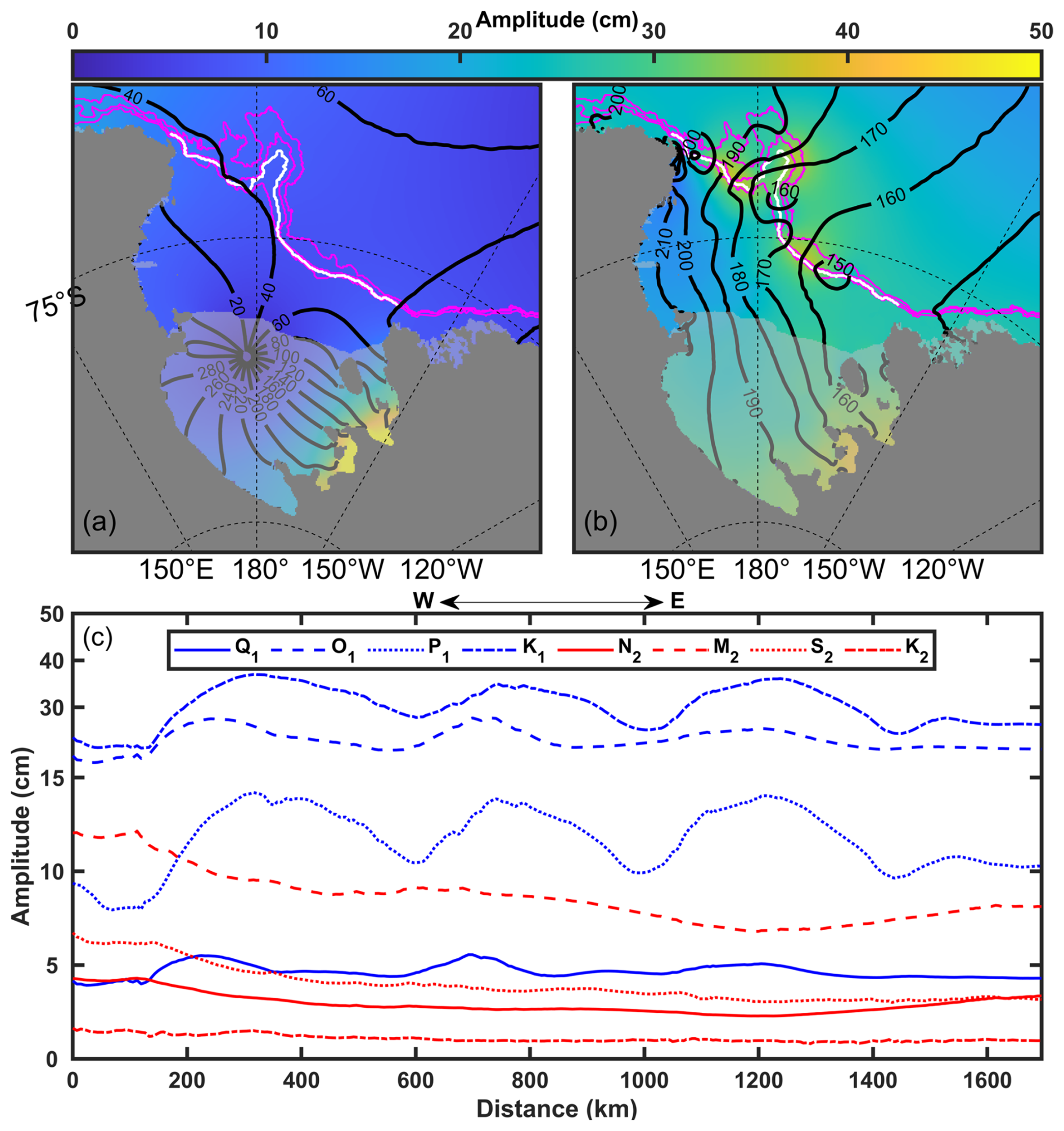
Figure 5 The cotidal charts of (a) M₂ and (b) K₁ tidal constituents from the model simulation. The co-phase lines are shown as black lines. The 500, 1000, and 2000 m isobaths (magenta) and the 700 m isobath (white) are shown along the continental slope. (c) The amplitude of individual constituents along the 700 m isobath.

In parallel to the tidal elevation patterns, the diurnal and semi-diurnal tides show pronounced differences in the barotropic tidal current fields (Fig. 6a and b). Over the continental slope, the K₁ constituent exhibits a complex flow regime with pronounced variations in both the magnitude and direction (see the shading and tidal ellipses in Fig. 6b). In agreement with Robertson et al. (2003), the M₂ tidal flow is generally weak throughout the Ross Sea (Fig. 6a), except in the vicinity of the south-eastern ice shelf grounding zone, where current speeds exceed 0.1 m s⁻¹. The mean amplitudes of tidal cross-slope velocities shown in Fig. 6c and d suggest that the strength of both the semi-diurnal and diurnal currents is related to the bottom topography. For diurnal tides, significant velocities form a banded structure along the slope, spanning the entire water column with bottom intensification and reaching up to 20 cm s⁻¹. The semi-diurnal tidal currents are also bottom-intensified as well, though their speeds are much weaker (∼5 cm s⁻¹). These patterns are linked to the eddy-like structures and bottom-trapped waves described in the following Sect. 3.2 and 3.3. In addition, a weak surface-intensified feature is found in Fig. 6c, which is likely induced by near-inertial winds (Brearley et al., 2017), as the local near-inertial frequency (∼0.08 cph) is close to the semi-diurnal tidal frequency.

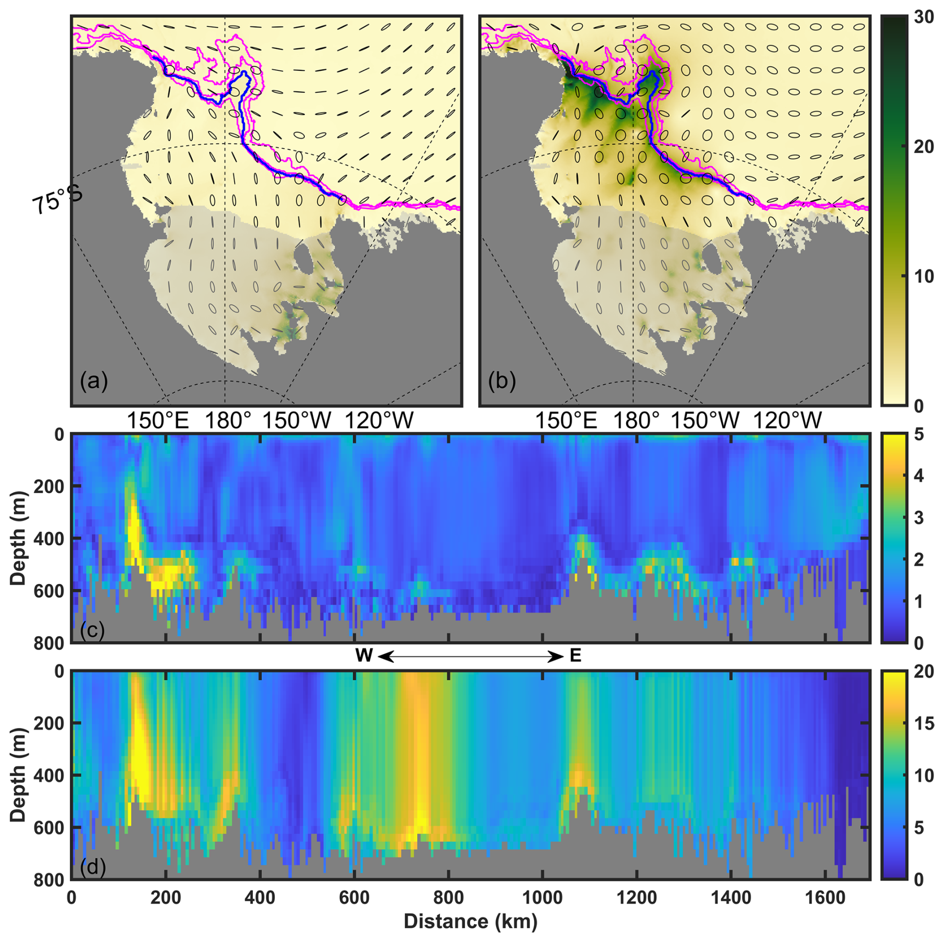
Figure 6 (a, b) Tidal ellipses for M₂ and K₁. Ellipse major axes are normalized; color shading shows actual speed (cm s⁻¹). The 500, 1000, and 2000 m isobaths (magenta) and the 700 m isobath (blue) are shown along the continental slope. (c, d) Vertical section of the mean amplitude of cross-slope tidal flow speed (cm s⁻¹) for the semi-diurnal and diurnal constituents along the 700 m isobath.

3.2 Eddy-like structures in the topographic mode

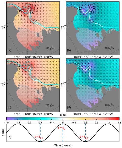
As described in Sect. 2.4, the barotropic tidal flow has been decomposed into the surface and topographic modes so as to elucidate how topography governs the flow structure. The decomposed topographic mode of diurnal tides, shown in Fig. 7a and b, exhibits three eddy-like structures over the continental slope, marked by distinct SSH anomalies. The direction of the flow, as well as the sign of the SSH anomalies, reverses between flood and ebb tides (Fig. 7a and b), indicating a direct dynamical coupling between them. However, according to the assumption of the decomposition framework, the topographic mode itself is nondivergent, and the SSH anomalies are only related to the surface mode. Given the conservation of water mass, the tide-induced change in sea level Δη over any period can be written as a function of the divergence of the tide-induced volume transport:

$$\begin{array}{}\text{(20)}& \mathrm{\Delta }\mathit{\eta }=\int \mathrm{\nabla }\cdot \left(H{\mathit{u}}_{\mathrm{S}}\right)\mathrm{d}t.\end{array}$$

Integration over the flood and ebb tidal periods reveals that the pattern of surface-mode transport divergence (Fig. 7c and d) closely matches the SSH pattern (Fig. 7a and b). This agreement confirms that the SSH anomalies arise from the surface mode. During the flood period, as the surface-mode tidal flow encounters the continental slope, it adjusts to the topography and generates three SSH maxima through convergence. In contrast, during the ebb period, the flow diverges over the slope, producing three SSH minima that mirror the flood-time pattern. Critically, for diurnal tides, the SSH anomalies can persist for 6 h, which is longer than the geostrophic adjustment timescale ($\mathrm{1}/f\approx \mathrm{2}$ h), thus allowing for the formation of eddy-like flows seen in the topographic mode. During the flood-ebb transition, tidal flows reverse, and eddy-like structures are no longer sustained as SSH anomalies diminish (Fig. S18 in the Supplement). They re-emerge only when the next tidal phase re-establishes the SSH gradient. For semi-diurnal tides, the tidal flow is much weaker, and its surface mode shows negligible divergence (Fig. 8c and d). This leads to no significant SSH anomalies over the slope (Fig. 8a and b). Additionally, the semi-diurnal flood/ebb period is likely too short for geostrophic adjustment to establish organized currents. Consequently, no eddy-like features appear in the topographic mode of semi-diurnal tides.

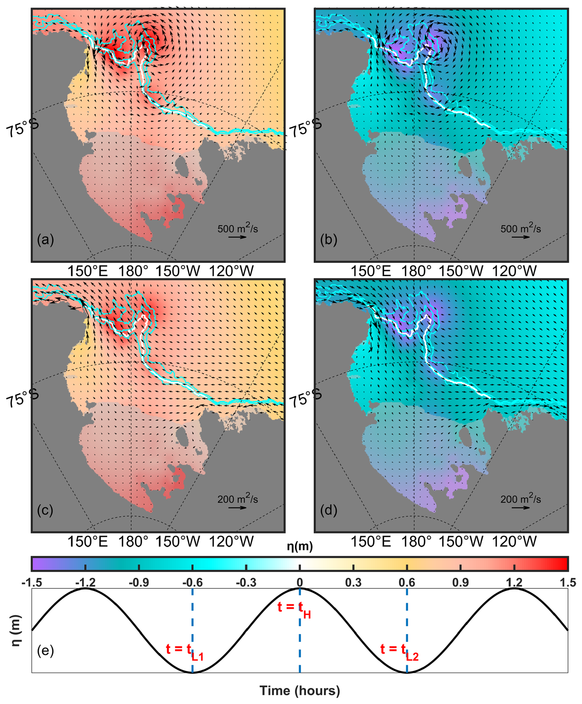
Figure 7 (a) Tide-induced sea level change (color shading) during flood period (from $t_{L_{\mathrm{1}}}$ to t_H), overlain by volume transport vectors of the topographic mode at t_H. (b) Tide-induced sea level change (color shading) during ebb period (from t_H to $t_{L_{\mathrm{2}}}$), overlain by volume transport vectors of the topographic mode at $t_{L_{\mathrm{2}}}$. (c, d) Corresponding volume divergence due to the surface mode (color shading) during flood and ebb periods, overlain by volume transport vectors of the surface mode at t_H and $t_{L_{\mathrm{2}}}$, respectively. The 500, 1000, and 2000 m isobaths (cyan) and the 700 m isobath (white) are shown along the continental slope. (e) Schematic for illustrating the flood and ebb periods for integration.

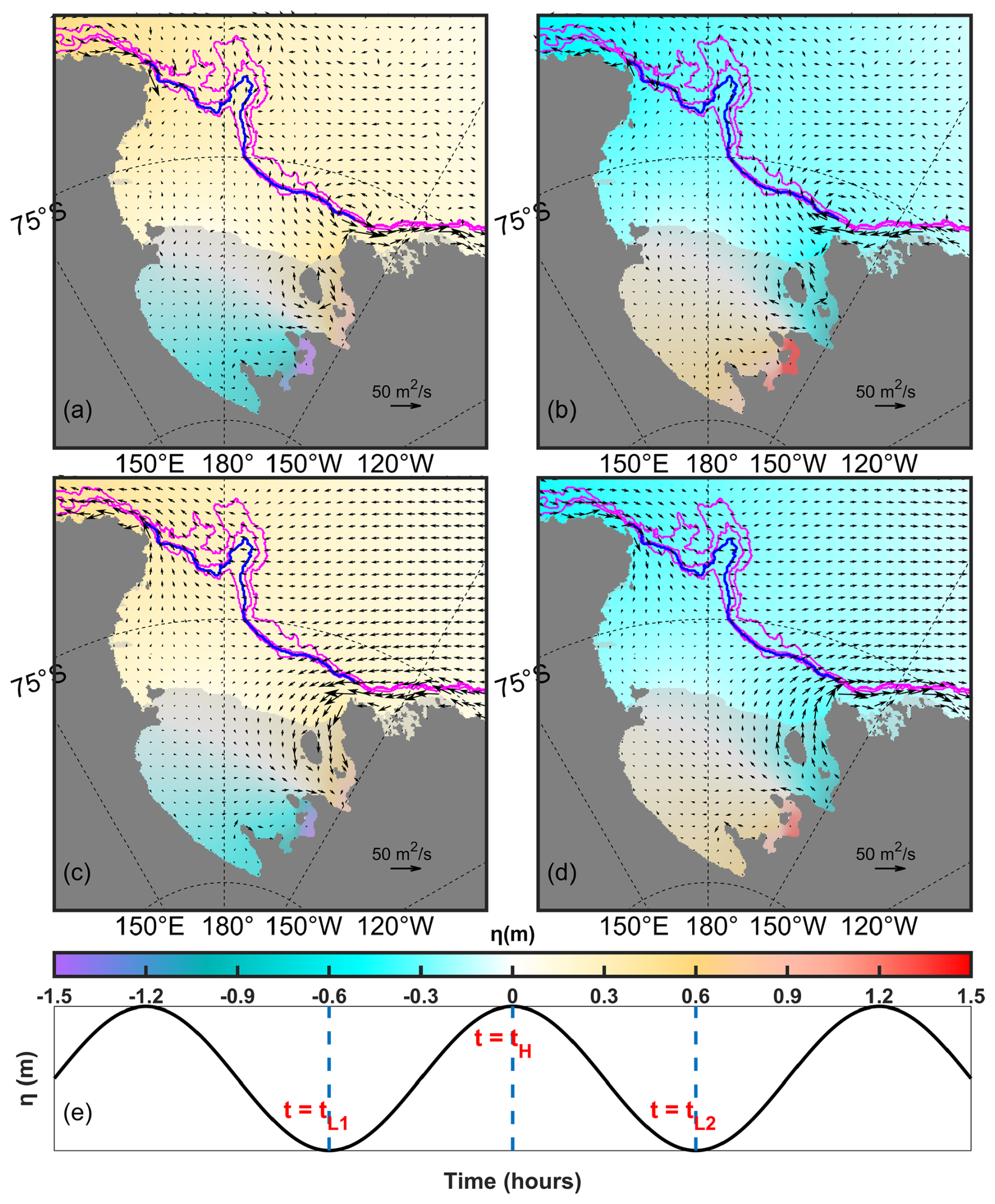
Figure 8 Same as Fig. 7, but for semi-diurnal tides.

Since the topographic mode dominates the tidal flow over the continental slope, it is instructive to quantify its role in cross-slope transport. The cross-slope volume (VT) and heat (HT) transport through the 700 m isobath are calculated as

$$\begin{array}{}\text{(21)}& {\displaystyle }\text{VT}={\int }_{\mathrm{0}}^L{\int }_{-H}^{\mathrm{0}}\mathit{u}\cdot {\displaystyle \frac{\mathrm{\nabla }h}{\left|\mathrm{\nabla }h\right|}}\mathrm{d}z\mathrm{d}l,\text{(22)}& {\displaystyle }\text{HT}={\int }_{\mathrm{0}}^L{\int }_{-H}^{\mathrm{0}}\mathit{\rho }{c}_p(T-T_{\mathrm{f}})\mathit{u}\cdot {\displaystyle \frac{\mathrm{\nabla }h}{\left|\mathrm{\nabla }h\right|}}\mathrm{d}z\mathrm{d}l,\end{array}$$

where u can be decomposed into the surface- and topographic-mode tidal velocity vectors, c_p=3994 $\mathrm{J}{\mathrm{kg}}^{-\mathrm{1}}\mathrm{°}{\mathrm{C}}^{-\mathrm{1}}$ is the specific heat capacity, T is the potential temperature, and $T_{\mathrm{f}}=-\mathrm{1.9}$ °C is the freezing point of seawater. Positive (negative) values of VT or HT indicate onshore (offshore) transport.

As shown in Fig. 9a–c, the topographic mode is the primary driver of local instantaneous transport, surpassing the surface mode in regulating shelf-basin exchange. Nevertheless, its integrated transport along the entire 700 m isobath is nearly zero, indicating that it does not contribute to a net cross-slope volume flux. Time averaging (Fig. 9g) further illustrates that the offshore volume transport by the topographic mode offsets the onshore transport by the surface mode so that the volume is conserved.

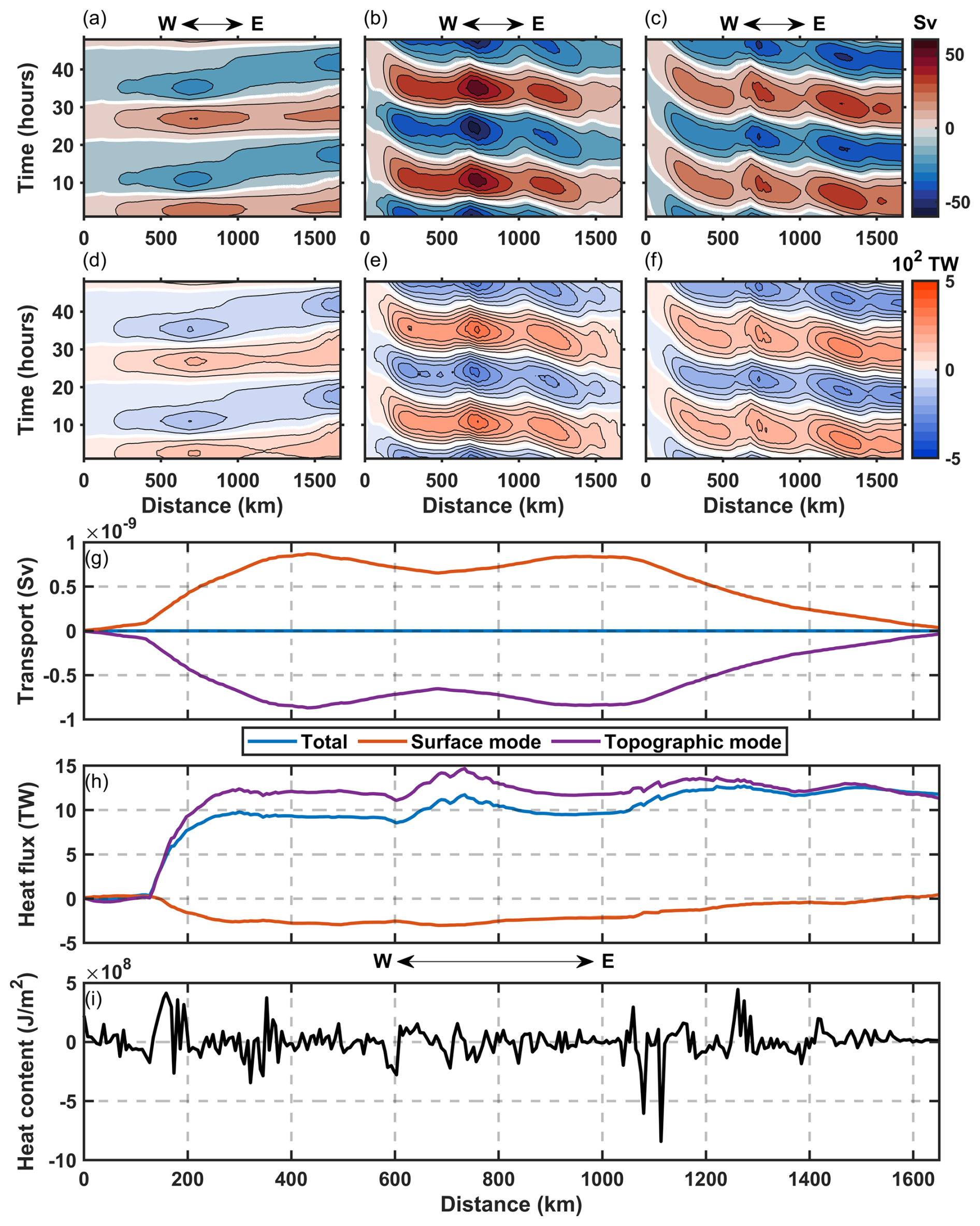
Figure 9 (a–c) Cross-slope volume transport integrated along the 700 m isobath as a function of time for (a) the surface mode, (b) the topographic mode, and (c) their sum. (d–f) The corresponding heat transport. (g, h) The temporal averages of the volume and heat transport, respectively. Positive (negative) values indicate onshore (offshore) transport. (i) Flood-minus-ebb heat content difference.

For cross-slope heat transport (Fig. 9d–f), the topographic-mode tides are even more influential, dictating local heat transport while also accounting for the majority of the instantaneous onshore flux. This is striking because, despite the absence of net volume transport, the tidal heat flux across the 700 m isobath can reach 12 TW, with most of which being attributable to the topographic mode (Fig. 9h). The mechanism for this tidal heat flux is preconditioned by a mean cross-slope thermal gradient (Fig. S19 in the Supplement), set up by warmer open-ocean waters abutting colder shelf waters. During flood tide, warmer water is advected across the slope onto the shelf, where it undergoes irreversible mixing with the ambient colder water. During ebb tide, the returning mixed water is colder than that advected onshore during flood tide, resulting in a flood-ebb difference in heat content on the slope. Although this difference varies spatially along the slope and even reverses locally, the regions with higher flood-tide heat content coincide with the strongest cross-slope velocities, primarily over the 100–200 km along-slope section (Figs. 9i, 6c and d). Since cross-slope heat transport scales with the product of velocity and thermal anomaly, the transport within the 100–200 km along-slope band overwhelms counter-gradient transport elsewhere, yielding a net onshore heat flux of 12 TW (Fig. 9h). Overall, these results highlight topographic-mode tides as a critical driver of cross-slope heat transport onto the Ross Ice Shelf, which potentially affects Antarctic ice-shelf melt and global sea-level rise.

3.3 Bottom-Trapped Waves and Energetics

3.3.1 Characteristics of Bottom-Trapped Waves

Since most of the Ross Sea lies poleward of both the diurnal (∼30° S) and semi-diurnal critical latitude (∼74.5° S) and its tidal regime is diurnal-dominated, internal tides generated by the barotropic tide-topography interaction are bottom-trapped, leading to an intensification of the near-bottom flow and shear (D'Asaro and Morison, 1992). As shown in Fig. 10a and b, both the baroclinic kinetic energy and squared vertical shear are intensified within the bottom tens of meters. This bottom-intensified tidally modulated shear is consistent with trapped internal tides. The vertical extent of these waves varies with the tidal cycle, increasing significantly during spring tide and shrinking or even vanishing during neap tide. Note that the term “bottom-trapped” refers to an energy maximum near the bottom, not the absence of baroclinic flow above it. These waves form through constructive interference of individual modes (Falahat and Nycander, 2015). It is also worth noting that similar near-bottom enhancements can arise from frictional boundary layer dynamics, nonlinear tidal rectification over rough topography (which also produces spring-neap variability), and topographic scattering or critical reflection.

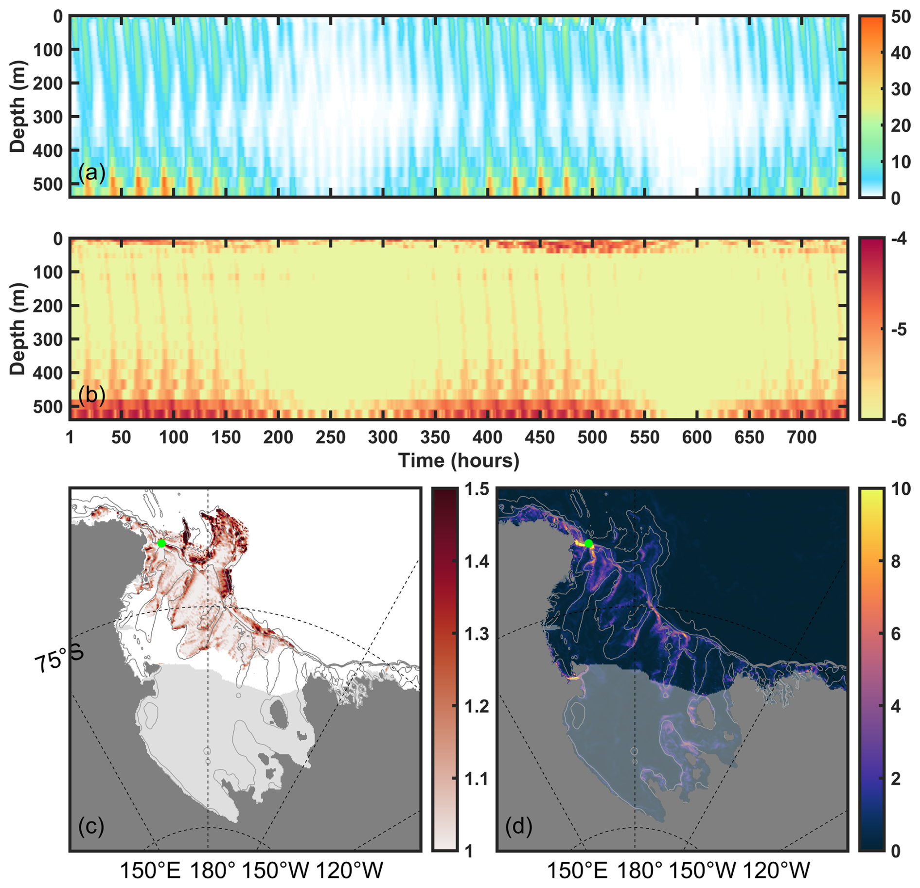
Figure 10 Time-depth plot of the (a) baroclinic kinetic energy density (J m⁻³) and (b) common logarithm of square of the vertical shear of tidal velocity ${\log }_{\mathrm{10}}(\frac{\partial u}{\partial z}{)}^{\mathrm{2}}+(\frac{\partial v}{\partial z}{)}^{\mathrm{2}}$ (s⁻²) at the point marked by green dots in panels (c) and (d) (close to mooring cc1) from the model simulation. (c) Map of the ratio of the near-bottom-averaged kinetic energy to the column-averaged kinetic energy (R_KE). (d) Map of the maximum vertical displacement (m) of time-averaged density at the bottom of each water column. Bathymetry contours are spaced at 500, 1000, and 2000 m.

To map the distribution of bottom-intensified energy, we introduce a non-dimensional parameter, R_KE, defined as:

$$\begin{array}{}\text{(23)}& R_{\text{KE}}=\langle E_{\mathrm{K}}{\rangle }_{\mathrm{100}}/\langle E_{\mathrm{K}}{\rangle }_H,\end{array}$$

where 〈E_K〉₁₀₀ and 〈E_K〉_H denote the kinetic energy averaged over the bottom 100 m and the full water column, respectively. The 100 m layer thickness is taken as a representative scale of the bottom-intensified layer, as revealed in Fig. 10a. The value of R_KE exceeds 1 indicates the presence of bottom intensification. To ensure the identified bottom-trapped signals are significant, we applied R_KE calculation only when the barotropic kinetic energy ranked in the top 10 % of the time-mean barotropic kinetic energy, equivalent to a velocity of 5 cm s⁻¹. The regions beneath ice shelves are excluded from the calculation.

The spatial pattern of R_KE in Fig. 10c reveals significant bottom intensification over the continental slope and topographic features such as banks and troughs, while it is minimal over the slope east of Houtz Bank (HoB). The bottom-trapped waves cause vertical displacement of bottom water particles, which peaks north of DT at meter-scale amplitudes (Fig. 10d). This is much smaller than the hundred-meter amplitudes of freely propagating internal tides (e.g., in the Bay of Biscay, see Pairaud et al., 2010), highlighting the bottom-trapped nature of Ross Sea internal tides.

A potential concern regarding the modal decomposition of Tanaka (2023) is that it assumes SSH is determined only by the surface mode, whereas in regions with strong stratification, SSH may also be affected by bottom-trapped waves. To test this, we evaluate the baroclinic pseudo sea level ζ_bc (Fig. S20a in the Supplement) with density, following McWilliams et al. (2024, their Eq. 17). Figure S20 shows that ζ_bc is negligible throughout the Ross Sea, even in the Drygalski and Joides Troughs where stratification is strongest. The mean amplitude of ζ_bc is less than 2 cm, more than an order of magnitude smaller than that of the barotropic SSH (Fig. S20b), thus the modal decomposition of Tanaka (2023) is valid in the Ross Sea.

3.3.2 Energetics

The energy conversion between the surface and topographic tidal modes is shown in Fig. 11a. A positive value denotes energy transfer from the surface to the topographic mode, and vice versa. As expected, the conversion is concentrated over topographic features, with the magnitude of 1 W m⁻², much greater than the BT-BC energy conversion rate (Fig. 11b). The pattern reveals large alternating positive and negative patches, which are associated with the eddy-like structures in the topographic mode (Fig. 7a and b). The conversion rate varies in sign along the slope because the eddies' velocities are alternately aligned with or against the surface mode (Fig. 7). In addition, smaller-scale patches are found along the coast, which are likely related to coastal trapped waves.

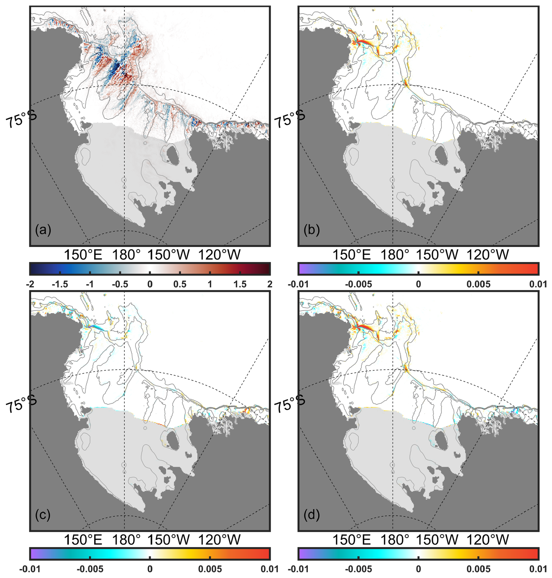
Figure 11 The rate of energy conversion (W m⁻²) from (a) Surface mode to Topographic mode, (b) Barotropic (Surface + Topographic modes) tides to baroclinic tides, (c) Surface mode to baroclinic tides, and (d) Topographic mode to baroclinic tides. Bathymetry contours are spaced at 500, 1000, and 2000 m.

Energy conversion from barotropic to baroclinic tides in the Ross Sea mainly occurs over the slope and peaks near the mouth of DT (Fig. 11b), with a rate of approximately 10⁻² W m⁻². The BT-BC conversion rate in the Ross Sea is considerably lower than those reported in other ocean regions, such as the ∼0.1 W m⁻² estimated in Monterey Bay (Kang and Fringer, 2012) and the ∼1 W m⁻² over the Luzon Ridge (Han and Eden, 2019), indicating weaker internal tide energy. This order of magnitude is consistent with the estimates of Müller (2013), who applied a global model and used a methodology similar to ours. It also agrees with the estimates derived from the method of Falahat and Nycander (2015), in which the rate is obtained by dividing the baroclinic energy density (Fig. 12b and d) by a decay time of 2–3 d. However, the model of Müller (2013) produces higher conversion rate near the Iselin Bank (IB) than our model. This discrepancy is likely due to the difference in horizontal and vertical resolution (Niwa and Hibiya, 2011). The energy conversion from barotropic to baroclinic tides is separated into contributions from the surface (Fig. 11c) and topographic modes (Fig. 11d), respectively. It is evident that the topographic mode dominates the conversion to baroclinic tides in most of the region. Notably, the surface mode appears to extract energy from the baroclinic tides, especially near the mouth of DT (negative values in Fig. 11c). This implies a cyclic energy pathway there: from the surface to the topographic mode, then to the baroclinic tides, and back to the surface mode.

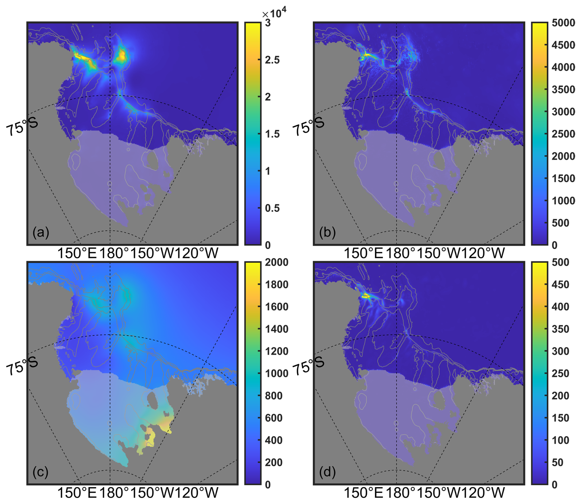
Figure 12 Spatial distribution of depth-integrated, period-averaged (a) barotropic kinetic energy density (J m⁻²), (b) baroclinic kinetic energy density (J m⁻²), (c) barotropic potential energy density (J m⁻²), and (d) available potential energy density (J m⁻²). Bathymetry contours are spaced at 500, 1000, and 2000 m.

Figure 12 presents the depth-integrated, period-averaged tidal energy densities in the Ross Sea. The total baroclinic energy densities (Fig. 12b and d) are of the same order as the theoretical estimates of Falahat and Nycander (2015), which are based on barotropic tidal velocities and topographic gradients. Overall, BTKE exceeds BCKE by an order of magnitude, which is supported by the low energy BT-BC conversion rate shown in Fig. 11b. Furthermore, the total tidal potential energy is itself an order of magnitude smaller than the kinetic energy, and within it, APE is an order of magnitude smaller than BTPE. The enhancement of BTKE along the slope is modulated by the topographic mode (Fig. 7a and b). Specifically, it is strongest where three eddy-like structures are present (Fig. 12a). Meanwhile, the enhancement of BTPE over the slope is associated with the surface mode of the diurnal tide (Fig. 12c). The APE reaches its maximum over the DT, corresponding to the vertical displacement shown in Fig. 10d. Although BCKE is relatively small in the depth-integrated sense, it is significant near the seafloor because baroclinic tides in the Ross Sea are predominantly bottom-trapped waves. Unlike freely propagating super-inertial internal tides that disperse energy into the ocean interior, these sub-inertial waves are trapped at the topography, confining their energy to the bottom boundary layer. This confinement of energy intensifies near-bottom velocity shear (D'Asaro and Morison, 1992), which promotes shear instabilities and turbulent dissipation, thereby enhancing local diapycnal mixing (Falahat and Nycander, 2015; Musgrave et al., 2017).

The barotropic and baroclinic energy fluxes exhibit remarkable differences in both magnitude and spatial pattern. For clarity, only the high-tide snapshots are displayed in Fig. 13. The complete figure set, covering time-average values, high-tide snapshots, and low-tide snapshots, is shown in Fig. S21 in the Supplement. The barotropic tidal energy flux is dominated by the pressure work (Fig. 13a), with the advective component being two orders of magnitude smaller (Fig. 13b). Both barotropic components are significantly shaped by the topographic mode but respond differently to tidal phase. The simultaneous sign change of sea surface perturbation and tidal velocity causes the pressure-work-induced energy flux to maintain a consistent direction over the slope (Figs. 13a and S21c). The advective flux, however, reverses direction between flood and ebb (Figs. 13b and S21f). Consequently, the time-averaged energy flux from pressure work retains eddy-like patterns along the slope (Fig. S21a), whereas the advective component is largely cancelled out (Fig. S21d).

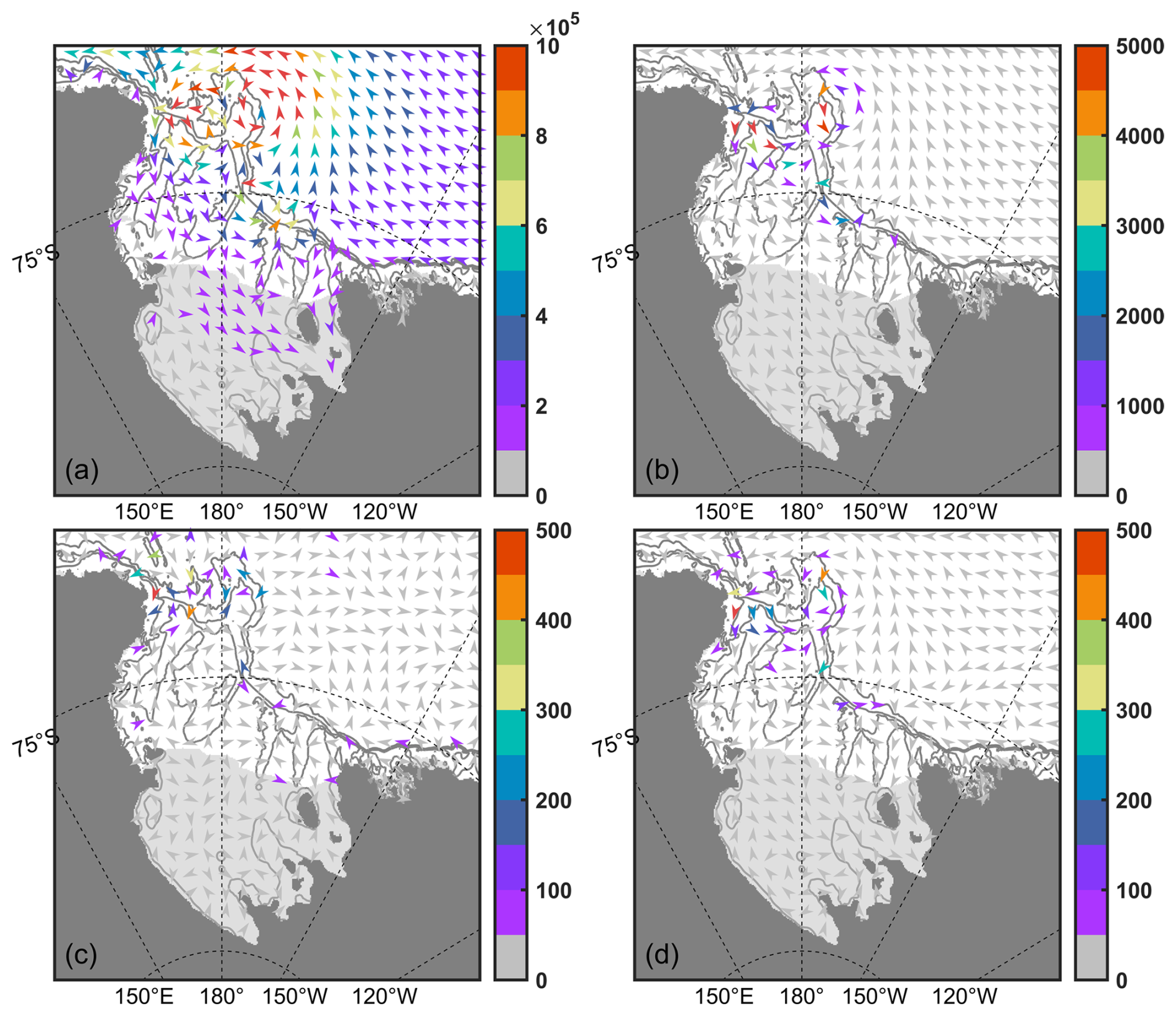
Figure 13 Depth-integrated energy flux (W m⁻¹) components (snapshots at high tide): (a) barotropic pressure work, (b) barotropic advective work, (c) baroclinic pressure work, and (d) baroclinic advective work.

The baroclinic energy fluxes from pressure work and advection are comparable in magnitude, peaking around the DT and IB (Fig. 13c and d) in a pattern consistent with the BCKE distribution (Fig. 12b). Moreover, the magnitude is consistent with that reported by Müller (2013) in the Ross Sea. The pressure-work-induced baroclinic energy flux exhibits a disorganized directional pattern (Fig. 13c). This disorder arises because bottom-trapped internal waves differ fundamentally from free-propagating waves, which radiate internal tide energy in coherent beams. In contrast, the velocity and pressure structures of bottom-trapped waves are governed by the topographic gradients and the distance from the generation site (Falahat and Nycander, 2015). Consequently, the irregularity of the topography induces a complex interference pattern as waves generated at sites overlap, ultimately leading to this disordered state.

Figure 14 shows the spatial distribution of total tidal energy dissipation, which is strongest along the continental slope, especially west of Cape Adare. Pronounced dissipation also occurs near the southwestern grounding line of the Ross Ice Shelf and over shelf regions with complex topography. A dedicated calculation of the baroclinic dissipation was not performed, owing to numerical constraints. Near the steep slope, C-grid staggering and partial bottom cells interact to treat some near-bottom velocity points as land, so that bottom cells over the slope often hold only one horizontal velocity component. Accordingly, bottom-intensified velocities may not be fully represented. This limitation affects the estimate of baroclinic energy flux divergence far more than baroclinic energy itself. Because the thin layer of bottom-intensified flow occupies only a minor portion of the 500–2000 m water column, the omission of one velocity component may lead to a slight underestimate of depth-integrated energy, with an uncertainty typically below 20 %. However, the baroclinic energy flux over upper layers of water column may partially cancel during vertical integration (as illustrated in Fig. S22 in the Supplement), and the near-bottom flux is comparatively strong and coherent. The integrated flux is therefore overwhelmingly determined by the lowest few partial cells and is highly sensitive to their velocity components. Missing either u^′ or v^′ in these cells projects the local flux vector onto a single direction, distorting both magnitude and orientation. Accordingly, diagnosing baroclinic dissipation as the residual would introduce significant numerical uncertainty that we do not report it separately. The estimated barotropic-to-baroclinic energy conversion is an order of magnitude smaller than the total dissipation shown in Fig. 14. Even if fully dissipated locally, this converted energy would represent only a minor fraction of the regional tidal energy budget. Thus, the conclusion that barotropic tides dominate the regional dissipation remains valid.

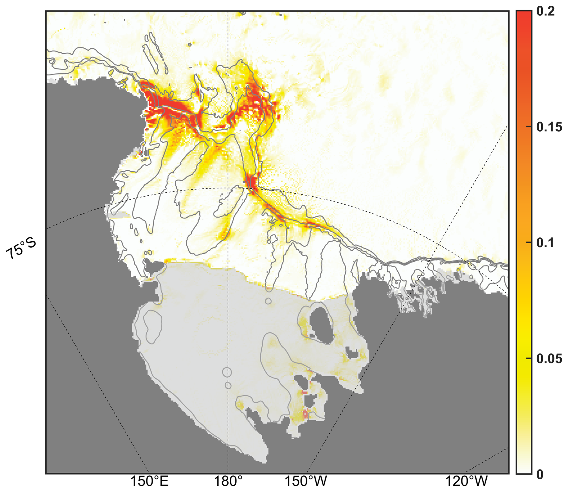
Figure 14 Map of the depth-integrated, period-averaged tidal dissipation rate (W m⁻²). Bathymetry contours are spaced at 500, 1000, and 2000 m.

4 Summary and discussions

Using a three-dimensional high-resolution regional model, we investigated the characteristics of tides in the Ross Sea, with a focus on the eddy-like topographic mode and bottom-trapped waves through modal decomposition and energy budget analysis. The model shows good agreement with observations in terms of both mean flows and tidal signals, although simulated tidal amplitudes are slightly weaker. Our results confirm a spatial pattern consistent with earlier work: diurnal tides dominate the continental slope, while both diurnal and semi-diurnal constituents are prominent in the south-eastern grounding zone beneath the ice shelf, where the semi-diurnal tide establishes an amphidromic point system.

On the continental slope, diurnal and semi-diurnal tides differ in tidal amplitude and current structure. Diurnal constituents exhibit three distinct amplitude peaks, absent in semi-diurnal tides. Semi-diurnal currents show bottom intensification, whereas diurnal currents display a more complex pattern with bottom intensification plus full-water-column enhancement. Modal decomposition of the diurnal tides shows that convergence and divergence of the surface-mode flow generate three SSH extremes along the slope. These SSH anomalies persist long enough for geostrophic adjustment, giving rise to three eddy-like structures in the diurnal topographic mode. Semi-diurnal tides exhibit no such features because they are too weak to generate SSH extremes, and their period is too short for geostrophic adjustment to occur. The topographic mode governs local cross-slope volume and heat transport, with a time-averaged onshore heat flux of ∼12 TW. Energy conversion between the surface and topographic modes reaches ∼1 W m⁻² along the slope.

Baroclinic tides in the Ross Sea, though an order of magnitude weaker in energy than barotropic tides, exist primarily as bottom-trapped waves over the slope, banks, and troughs. They drive several meters of vertical displacement and generate a near-bottom shear layer tens of meters thick. This layer expands during spring tides and nearly vanishes during neap tides. Energy budget analysis reveals that the barotropic-to-baroclinic conversion rate in the Ross Sea is only ∼0.01 W m⁻², much weaker than values reported for other oceans (e.g. Kang and Fringer, 2012). Barotropic tidal energy flux is dominated by pressure work, with advection an order of magnitude smaller; its spatial patterns are strongly modulated by the topographic mode. In contrast, baroclinic energy fluxes from pressure work and advection are comparable, indicating significant nonlinearity within the internal tide field. These fluxes peak near Drygalski Trough and Iselin Bank. Strong tidal dissipation (∼0.1 W m⁻²) occurs along the slope, mainly attributed to barotropic tides, as internal tide energy is too weak to contribute appreciably to the total dissipation.

The topographic mode identified in this study may drive along slope rectification that perturbs the density field, triggering geostrophic adjustment which could sustain the Antarctic Slope Current and modulate its acceleration (Stewart et al., 2019), offering a possible explanation for its spatial heterogeneity (Liu et al., 2025). Onshore tidal heat flux associated with topographic control may influence ice shelf basal melting, with potential consequences for ice shelf stability. Bottom trapped baroclinic tides over the slope may enhance mixing and water mass transformation; together with the topographic mode, they could regulate cross slope exchange and export of AABW and DSW. In winter, the eddy-like structures of the topographic mode might alter the distribution of sea ice, which could in turn modify sea surface momentum input and upper ocean stratification through ice-ocean feedbacks. Overall, these tidally driven processes may exert broader influences on the regional ocean-cryosphere system, with potential implications for its response to climate change.

This study has some limitations. First, the small Rossby radius of deformation in the Ross Sea (Chelton et al., 1998; Hallberg, 2013) requires a model horizontal resolution finer than 1 km to fully resolve mesoscale eddies (Padman et al., 2009). Although barotropic tidal heat flux is largely insensitive to horizontal resolution, internal tide generation and its contribution to heat flux may be altered by finer grids through better resolved small-scale topography. Finer grids may also better capture nonlinear interactions between internal tides and mesoscale eddies, which can modulate the spatial redistribution of tidal energy and indirectly affect heat flux patterns. Owing to the poor representation of mesoscale eddies, our model may have overestimated tidal heat transport across the continental slope, as eddies would otherwise contribute to this transport. A further limitation of the model is that its 30 m vertical resolution at 500 m depth is insufficient to adequately resolve the near-bottom (≤50 m) velocity enhancement related to the trapped baroclinic tides. Insufficient vertical resolution is known to underestimate higher-mode energy and vertical shear (Hiron et al., 2025), and consequently baroclinic dissipation. Moreover, energy conversion is modulated by background stratification (Varlamov et al., 2015), and this sensitivity spans scales from fortnightly fluctuations (Zhang et al., 2021) to decadal trends (Opel et al., 2024). For sharp stratification gradients, coarse vertical resolution introduces more than 30 % errors in these dynamics (Song and Chen, 2020). Si et al. (2023) examined the resolution dependence of tidal heat advection, while their analysis focused on the fresh-shelf regime rather than dense-shelf regions like the Ross Sea. Higher horizontal and vertical resolution is needed for a complete picture of tidal energetics and heat transport in the Ross Sea.