Impact of wind variations on surface variability over the Patagonian Continental Shelves

We study the impact of wind variability on sea surface temperature (SSTa), sea surface salinity (SSSa), and sea level anomaly (SLAa) over the Patagonian shelves around southern South America using satellite observations and the ERA5 reanalysis. Using Empirical Orthogonal Function (EOF) analysis, we identify the dominant patterns of variability in surface ocean properties and winds and assess their interconnections through correlation and composite maps. Zonal and meridional wind anomalies modulate the variability of sea level anomaly with distinct spatial signatures. Meridional wind variability emerges as the dominant driver, exerting a strong influence on sea surface temperature, salinity, and sea level, generating coherent patterns across the southeast South Pacific and southwest South Atlantic continental shelves. Specifically, the leading mode of meridional wind is significantly correlated with the dominant modes of SSTa, SSSa, and SLAa variability. Moreover, the spatial patterns emerging from the composites associated with the leading meridional wind mode are consistent with the dominant SSTa, SSSa, and SLAa variability patterns. These results suggest that southerly winds promote upwelling and offshore flow of low salinity waters over the Pacific shelf, weaken the southward flowing Cape Horn Current along the shelf break, and strengthen the northward transport of cold-salty subantarctic water over the Atlantic shelf. Northerly winds reverse these dynamics. This study provides evidence of wind-driven coupling of the shelf circulation around southern South America and the interocean exchanges between the Pacific and Atlantic continental shelves.

1 Introduction

Wind forcing is a key driver of ocean circulation, playing a crucial role in the transport and distribution of water masses over continental shelves. The variability of surface winds modulates the circulation patterns, vertical mixing, nutrient supply, sediment transport, and overall water properties. These processes are particularly relevant on continental shelves, where wind-driven dynamics interact with bathymetric features and coastal morphologies, shaping regional environmental conditions and ecosystem structures (e.g. Simpson and Sharples, 2012; Brink, 2023).

The continental shelf around southern South America, encompassing the southwest Atlantic and southeast Pacific, forms a highly productive system connected by interocean exchanges (Marrari et al., 2017; Matano et al., 2019; Guihou et al., 2020). Although previous studies have characterized broad circulation patterns and the main forcing mechanisms governing the shelf region across various timescales, key aspects of the regional variability and the mechanisms controlling them remain poorly understood, particularly south of 40° S, where observational and modelling efforts are comparatively scarce. Hereafter, we refer to the continental shelves south of 40° S as the Patagonian Continental Shelves (PCS), distinguishing between their Pacific and Atlantic regions (Fig. 1).

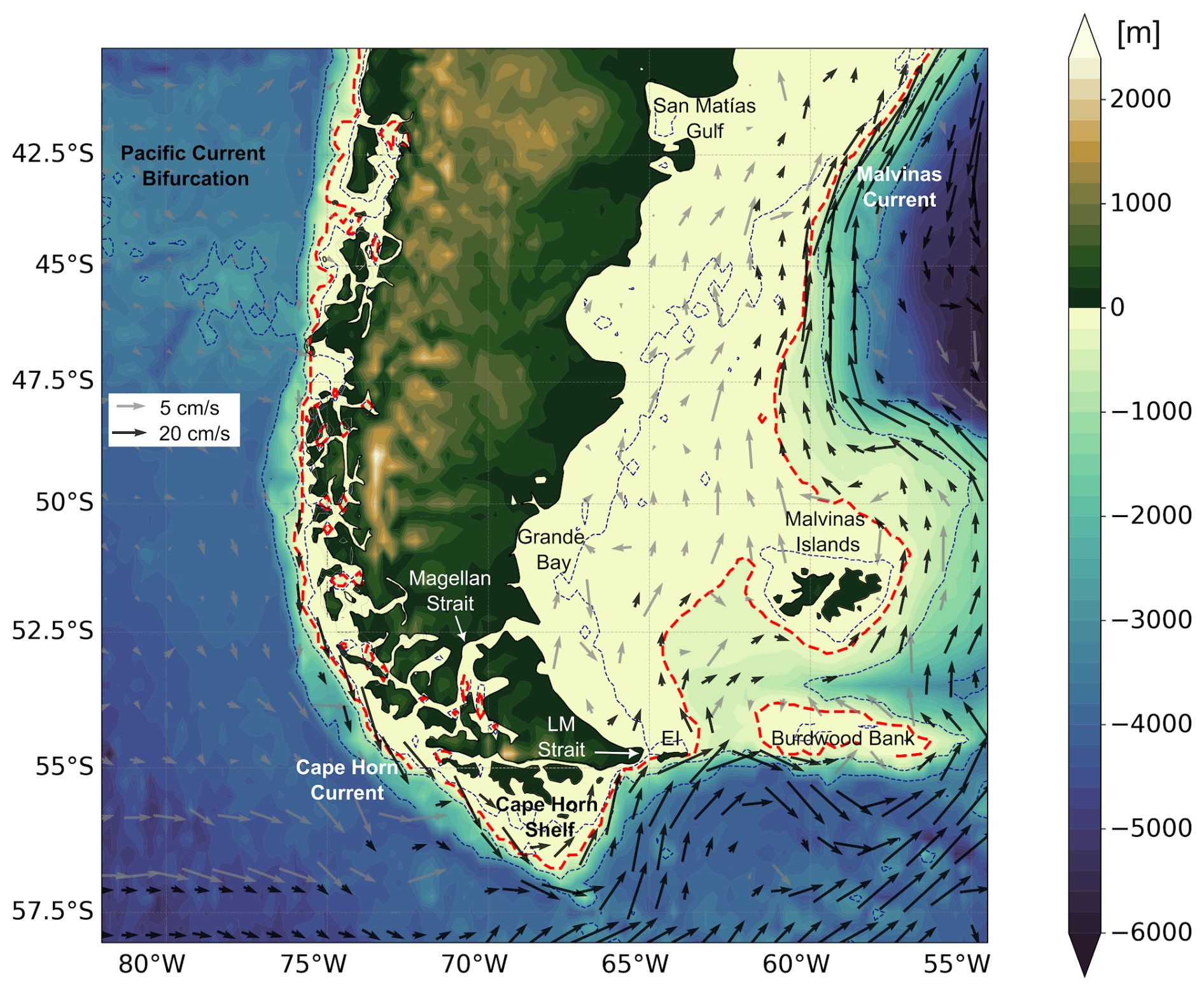
Figure 1 Mean circulation around South America inferred from the Mean Dynamic Topography for the period 1993–2022. Gray arrows indicate velocities lower than 8 cm s⁻¹, and black arrows indicate velocities greater than 10 cm s⁻¹. Note the different scales. Colours show bathymetry (yellow and blue) and land topography (green and brown), in meters. Bathymetry data are from GEBCO Bathymetric Compilation Group (2023). The red dashed line marks the 200 m isobath, close to the continental shelf break. Blue dashed lines indicate the 100, 1000, and 3000 m isobaths. LM: Le Maire Strait. EI: Estados Islands.

1.1 The Pacific Patagonian Shelf

The Pacific PCS is relatively narrow, averaging ∼ 40 km in width, except at its southernmost extension near Cape Horn, where it expands to roughly 120 km. The coastline is highly irregular, characterized by a complex network of fjords, channels, estuaries, and islands, which define the southern Pacific coast. These fjords, typically 100–500 m deep and tens of kilometres long, are strongly stratified by a halocline at 4–20 m (Silva et al., 1997; Cáceres et al., 2002). Bathymetric gradients are steep, and the shelf is intersected by submarine canyons and sills that influence the circulation and vertical mixing (Farmer and Freeland, 1983; González et al., 2011; Inall and Gillibrand, 2010; Stigebrandt, 2012). The region experiences strong westerly and northwesterly winds, frequent storms, and high precipitation, which, combined with freshwater inputs from rivers and glacial melt, generate significant spatial and temporal variability in temperature and salinity (Dávila et al., 2002; Garreaud et al., 2013; Iriarte et al., 2017; León-Muñoz et al., 2024). These geographic and climatic features strongly modulate coastal currents, upwelling intensity, and the distribution of nutrients, shaping both physical and biological conditions of the shelf (e.g., Silva and Neshyba, 1979; Iriarte et al., 2007; González et al., 2011; León‐Muñoz et al., 2013).

The South Pacific Current flows eastward and bifurcates near 40–45° S upon reaching the Chilean coast, forming the northward-flowing Humboldt Current and the southward-flowing Cape Horn Current (Strub et al., 2019; Wooster and Reid, 1963; Zheng et al., 2023). The latitude of bifurcation shifts with wind forcing and climate variability, which strongly influences the distribution of water masses and upwelling intensity along the Chilean margin (Strub et al., 2019). South of 45° S, the Cape Horn Current transports cold and relatively fresh Subantarctic Surface Water poleward, which mixes with freshwater from rivers and glacial melt to form Modified Subantarctic Waters (∼ 32; Saldías et al., 2024). The Cape Horn Current continues eastward south of Tierra del Fuego, with part of its flow entering the Atlantic shelf through the Le Maire Strait and the gap between Estados Island and Burdwood Bank (Fig. 1), while the remainder merges with the northern Antarctic Circumpolar Current. This region thus represents a critical junction where Pacific, Atlantic, and Southern Ocean waters interact, shaping regional circulation and biogeochemical exchanges.

At seasonal timescales, the circulation over the Pacific shelf is influenced by meridional migrations of the South Pacific anticyclone, altering the direction of alongshore winds between 34 and 45° S. This generates large-scale adjustments in coastal sea level and currents, modulating the shelf circulation and seasonal upwelling variability (Strub et al., 2019). Satellite altimetry reveals a strong seasonal reversal in geostrophic transport between 40 and 48° S, while the Cape Horn Current exhibits weaker seasonality south of 48° S (Saldías et al., 2024). Studies suggest that this seasonality is driven by a buoyancy-driven current off northern Patagonia and by the influence of local wind stress (Guihou et al., 2020; Saldías et al., 2024).

At interannual scales, sea level variability in the Pacific between 38 and 46° S is strongly correlated with El Niño Southern Oscillation (ENSO) (Strub et al., 2019), and local meridional winds also force alongshore currents (Strub et al., 2019; Guihou et al., 2020). In addition, the Southern Annular Mode (SAM) modulates the wind stress and surface circulation, with opposite effects along the Chilean margin: positive SAM phases enhance equatorward coastal transport north of ∼ 40° S, while south of ∼ 45° S they reinforce poleward flow (Strub et al., 2019). Altimetric observations show interannual fluctuations in Cape Horn Current transport of 0.8–3.4 Sv south of 40° S (Zheng et al., 2023), though their relationship with ENSO or SAM is unclear. Guihou et al. (2020), however, suggest that SAM modulates the wind variability and hence the Cape Horn Current transport.

1.2 The Atlantic Patagonian Shelf

The Atlantic PCS is broad with a gradual bathymetric gradient, ranging from ∼ 450 km wide near 40° S to ∼ 850 km at 51° S. The coastline is comparatively smooth, dominated by wide bays, gulfs, and estuarine systems rather than fjords and channels characteristic of the Pacific margin. The eastern edge of this vast shelf is the slope characterized by an abrupt bathymetric gradient. Circulation on the Atlantic Patagonian Shelf is influenced by multiple forcings. Strong westerly winds, with climatological surface stress around 0.15 Pa (Palma et al., 2008), dominate the dynamics south of 40° S and generate a mean northeastward flow. Tides in this region reach exceptionally high amplitudes, exceeding 10 m in parts of Tierra del Fuego and along the Atlantic coast, as the continental shelf behaves like a semidiurnal resonant basin. This resonance sustains unusually large tidal amplitudes (Webb, 1976; Glorioso and Flather, 1995, 1997; Dinápoli and Simionato, 2025b), enhancing vertical mixing and often eroding vertical stratification across a broad coastal band, even during summer (Romero et al., 2006). Another critical factor is the input of low-salinity waters. Most of this buoyancy is derived from the Pacific Ocean, as direct continental runoff into the South Atlantic is limited to very few rivers of relatively small discharge. These fluxes freshen the southern shelf and contribute to the formation of the coastal low-salinity tongue historically referred to as the Patagonian Current, with buoyancy fluxes further modulating circulation and water column structure (Palma et al., 2008; Palma and Matano, 2012; Brun et al., 2020).

The mean circulation in the Atlantic PCS is predominantly northeastward. These waters, referred to as South Atlantic Subantarctic Shelf Waters, are of Subantarctic origin mixed with continental runoff, primarily from inflows from the southeast South Pacific, resulting in salinities of 32.5–33.9, except in the San Matías Gulf, where salinity exceeds 34 (Brun et al., 2020; Martinez et al., 2023). Along the slope, the Malvinas Current flows northward, transporting cold and relatively high-salinity waters (∼ 34.2) (Fig. 1). Near 40° S, wind forcing is a major driver of the flow variability on the Atlantic PCS. Direct observations show that the along-shelf current variability is coherent in the cross-shelf direction and largely barotropic, with ∼ 50 % of the velocity variance explained by along-shelf wind fluctuations. These winds induce volume transport variations between −5 Sv (southwestward) and +11 Sv (northeastward), with a mean northeastward flow of 2.65 ± 0.07 Sv (Lago et al., 2019, 2021). At seasonal scales, the Atlantic shelf transport south of 40° S appears to be controlled by interactions between onshore mass fluxes from the Drake Passage and local wind stress. Notably, local winds are often out of phase with transport variability (Combes and Matano, 2018; Brun et al., 2020). Though few studies address the intraseasonal circulation variability, Juhl et al. (2024) demonstrate that sea surface height variations over the Atlantic PCS are associated with alongshore wind variability. Ocean reanalyses and numerical models indicate that at interannual scales winds are the primary driver of the circulation south of 40° S and that these variations are influenced by both the SAM and ENSO (Combes and Matano, 2018; Guihou et al., 2020; Bodnariuk et al., 2021).

1.3 Aims of this study

We propose that meridional wind fluctuations modulate along-shelf circulation through Ekman dynamics, inducing cross-shelf pressure gradients that alter along-shelf transport. Because the mean flow is southward in the Pacific and northward in the Atlantic, spatially uniform meridional winds blowing over both shelves should enhance transport on one margin and weaken it on the other, potentially reshaping inter-ocean exchange and the relative contributions of Subantarctic Water and low-salinity Pacific inflows. Although such transport variations likely affect regional temperature, salinity, and biogeochemical properties, few studies have addressed the shelf system as a whole, hindering our understanding of inter-ocean connectivity and its implications on the circulation, biogeochemistry, and species distribution.

The aim of this study is to analyse the response of the continental shelf around southern South America to changes in wind forcing, its potential impact on the connectivity between the Atlantic and Pacific shelves, and on the changes in property distributions. By considering the PCS as an interconnected system spanning the Pacific and Atlantic margins, this study aims to advance the understanding of the dynamics of the PCS and their role in regional scale variability. Following this introduction, the paper is organized as follows: Sects. 2 and 3 describe the data sources and methods employed; Sect. 4 presents the main results; Sect. 5 develops the discussion; and Sect. 6 summarizes the key findings and conclusions.

2 Data

2.1 Reanalysis data: Wind

To study the wind effect, we used the fifth generation of climate reanalysis data (ERA5) generated by the European Centre for Medium-Range Weather Forecasts (ECMWF; Hersbach et al., 2020). The data are available at a 0.25° × 0.25° grid resolution with global coverage from 1940 to the present. ERA5 offers hourly data on 37 pressure levels, but for our analysis, we use daily average data at the surface level. ERA5 combines global observations with coupled numerical models of the climate system. It is widely used by the climate research community and performs well when compared with direct wind observations collected on the continental shelf in the Southwestern Atlantic (Risaro et al., 2022).

2.2 Satellite observations: Temperature, salinity, and sea level

Satellite-derived Sea Surface Temperature (SST) was obtained from an Optimal Interpolation (OI) based on microwave and infrared data (MW_IR) developed by Remote Sensing Systems. The Level-4 MW_IR OI SST product combines the through-cloud capabilities of microwave observations with the higher spatial resolution of infrared measurements near the coast. It provides global daily fields at 9 km resolution from June 2002 to the present. We chose this product combining microwave and infrared observations to reduce the impact of spurious variations induced by the relatively high mean cloud frequency, exceeding 50 % (e.g., Wilson and Jetz, 2016), which preclude deriving sea surface temperature from infrared observations.

Remote sensing measurements of Sea Surface Salinity (SSS) were obtained from a product generated by the European Space Agency Climate Change Initiative (ESACCI), which combines measurements from the Soil Moisture and Ocean Salinity (SMOS), Aquarius, and Soil Moisture Active Passive (SMAP) missions (Boutin et al., 2025). These data were resampled at daily and 0.25° × 0.25° resolution and are available from 2010 to 2023. Based on a comparison with in-situ CTD observations across nine satellite products, this product exhibits the best performance, especially in the southern sector of the Atlantic continental shelf (S. Basañes, personal communication, 2025). Use of satellite-borne SSS data is particularly challenging due to degraded sensitivity at low temperatures and land contamination close to shore (e.g. Grodsky et al., 2018) therefore, the SSS results should be interpreted with caution, particularly over the narrow SE Pacific shelf.

We used satellite Sea Level Anomaly (SLA) data from a 0.25° × 0.25° gridded product with a daily resolution of multi-satellite altimetric measurements collected from 1993 to the present. The data are distributed by the Copernicus Climate Change Service (C3S). SLA is derived from Absolute Dynamic Topography (ADT), which represents sea surface height relative to the geoid, and is referenced to the Mean Dynamic Topography (MDT) (ADT = SLA + MDT), where MDT represents the time-averaged sea surface height above the geoid in the period 1993–2012. SLA was used to calculate anomalies relative to the climatological cycle, while ADT was used to calculate the mean field and estimate surface absolute geostrophic velocities for the entire time period. Satellite-derived SLA can have increased uncertainties in coastal and shallow shelf waters and should therefore be interpreted with caution (Birol et al., 2025; see Sect. 5).

3 Methodology

3.1 Spatial domain

This study focuses on the Patagonian continental shelves around southern South America. To exclude the Brazil–Malvinas Confluence, a region characterized by high mesoscale variability in the southwest South Atlantic, we focused on the region west of 55° W and south of 40° S (Fig. 1). The northern boundary at 40° S also excludes the Río de la Plata outflow, a major source of low-salinity waters that are distinct from Subantarctic Shelf Water sources that occupy most of the Atlantic PCS. In the southeast Pacific, this northern latitude includes the region of divergence of the eastward flow of subantarctic waters reaching the continental shelf near 44–45° S. To analyse the property variability, the open ocean was masked, and the analysis was restricted to bottom depths shallower than 2800 m. While the emphasis is on the shelf dynamics, the domain was extended offshore beyond the shelf break to capture the southward flow associated with the Cape Horn Current (Chaigneau and Pizarro, 2005), and the northward Malvinas Current, which may influence the shelf circulation (e.g., Matano et al., 2010).

3.2 Temporal domain and preprocessing

The analysis spans from June 2002 to June 2023 for all variables, except SSS, which is only available after 2010. All datasets were analysed at daily temporal resolution. To focus on variability at intraseasonal to interannual timescales, a set of temporal preprocessing steps was applied consistently to all variables. All preprocessing steps were applied to the full available records of each dataset prior to restricting the analysis period in order to minimize boundary artifacts associated with digital filtering.

3.2.1 Detrending and removal of high-frequency variability

Prior to further analysis, all time series (SST, SSS, SLA, and the zonal and meridional wind components U and V) were linearly detrended and filtered to remove high-frequency variability. Detrending was carried out to minimize the impact of long-term changes, particularly warming and associated sea level rise. A second-order Butterworth low-pass filter with a cutoff period of 20 d was applied. Butterworth filters are characterized by a maximally flat frequency response in the passband, providing a smooth transition between retained and attenuated frequencies without spurious oscillations (Butterworth, 1930; Thomson and Emery, 2014). The 20 d cutoff was selected to suppress synoptic-scale variability while retaining intraseasonal to interannual signals. This choice reflects the effective temporal resolution of satellite SLA and SSS products, which do not reliably resolve variability at periods shorter than ∼ 20 d (Ferrari et al., 2017; Ballarotta et al., 2019). A second-order filter was chosen as a compromise between frequency selectivity and temporal fidelity, minimizing edge effects while efficiently attenuating high-frequency energy.

3.2.2 Removal of the seasonal cycle and definition of anomalies

Seasonality was removed using a fourth-order Butterworth band-stop filter with cutoff periods between 150 and 400 d. Higher-order filters provide a sharper separation of frequency bands but at the cost of stronger edge effects and increased distortion near the cutoff frequencies. The use of a fourth-order filter allowed for an efficient suppression of the seasonal band. Because such filters may introduce transient effects near the beginning and end of the records, particular care was taken in the interpretation of low-frequency variability and in subsequent spectral analyses. Alternative approaches to remove the seasonal cycle were also explored, including the subtraction of a daily climatology and harmonic analysis. While these methods effectively remove the mean seasonal signal, they retain residual variance within the seasonal frequency band. In contrast, the band-stop filtering approach ensures the removal of variability across the entire seasonal range. To assess the sensitivity to preprocessing, we tested alternative filtering approaches, including low-pass cutoffs of 10 and 30 d, a 20 d Lanczos low-pass filter, a second-order band-stop filter, and alternative seasonal cycle removal methods based on a smoothed daily climatology or annual and semi-annual harmonics. The main spatial patterns and relationships discussed in this study remained robust across these different preprocessing choices (Figs. S1–S5 in the Supplement). Hereafter, the resulting filtered time series are referred to as SSTa, SLAa, SSSa, Ua, and Va, corresponding to anomalies of SST, SLA, SSS, zonal wind, and meridional wind, respectively.

3.3 Analysis methods

3.3.1 Empirical Orthogonal Functions

To analyse the space-time variability of SSTa, SSSa, SLAa, and wind anomalies (Ua and Va) over the continental shelves around southern South America, we use Empirical Orthogonal Functions (EOF). EOF analysis decomposes the data into a set of orthogonal spatial patterns (EOFs) and associated temporal coefficients, called Principal Components (PCs), that maximize the explained variance of the dataset. The PCs describe the temporal evolution of each mode and are mutually uncorrelated at zero lag. These properties do not imply statistical independence or a one-to-one correspondence between EOF modes and independent dynamical processes (Monahan et al., 2009). For each variable, we computed the first three EOF modes of variability. The analysis focuses on the first two modes, which represent the dominant regional patterns of variability. The third mode explains only a small fraction of the total variance and was therefore not considered further. Additionally, we analysed the PC time series of the retained modes to investigate their temporal variability and explore their covariability.

3.3.2 Spectra

To analyse the frequency-domain variability of the leading modes of each variable (PC1 and PC2 derived from the EOF analysis), power spectral density estimates were computed using Welch's method. This approach segments the time series into overlapping sections, applies a windowing function to reduce spectral leakage, and then averages the periodograms of each segment to obtain a more stable estimate of the spectrum (Welch, 1967; Thomson and Emery, 2014). A Hann window was applied to each segment. The segment length was set to one-fourth of the total time series length $\left(n_{\mathrm{perseg}}=\frac{N}{\mathrm{4}}\right)$, with a 50 % overlap between segments. This configuration provides a compromise between frequency resolution and statistical stability and is frequently used for identifying broad spectral bands of variability rather than narrow spectral peaks. For visualization purposes, spectra are presented in a variance-preserving form. Confidence intervals at the 95 % level were obtained using the chi-square distribution with effective degrees of freedom computed following Thomson and Emery (2014), as defined in Eq. (1).

$$\begin{array}{}\text{(1)}& \mathit{\nu }=\mathrm{2}P,P={\displaystyle \frac{\mathrm{8}}{\mathrm{3}}}\cdot {\displaystyle \frac{N}{\left(\frac{n_{\mathrm{perseg}}}{\mathrm{2}}\right)}}\end{array}$$

where ν is the number of effective degrees of freedom used to define the chi-square confidence intervals, P is the effective number of periodogram estimates averaged, N is the number of data points in the time series, and nperseg is the length of each segment ($n_{\mathrm{perseg}}=N/\mathrm{4}$). The factor $\mathrm{8}/\mathrm{3}$ accounts for the variance reduction associated with the Hann taper and the 50 % overlap between consecutive segments (Thomson and Emery, 2014).

3.3.3 Linear correlations and composite analysis

Linear relationships between principal components and between wind and oceanic variables were quantified using the Pearson correlation coefficient. Because temporal filtering reduces the number of statistically independent observations, an effective sample size (N_eff) was estimated for each pair of time series by accounting for their autocorrelation structure, following the framework discussed by Bretherton et al. (1999). The effective sample size was computed using Eq. (2).

$$\begin{array}{}\text{(2)}& N_{\mathrm{eff}}={\displaystyle \frac{N}{\mathrm{1}+\mathrm{2}\sum _{k=\mathrm{1}}^K{r}_x\left(k\right)r_y\left(k\right)}}\end{array}$$

where N is the number of overlapping observations, and r_x(k) and r_y(k) are the autocorrelation functions of the time series at lag k. The summation, whose upper limit is K, was truncated at the first lag for which either autocorrelation became non-positive to avoid overestimating persistence.

Statistical significance was then evaluated using a two-tailed Student's t-test with N_eff−2 degrees of freedom (Wilks, 2011). Critical correlation thresholds were derived from the corresponding t distribution, and correlations exceeding this threshold were considered statistically significant. Given the relatively large effective sample sizes, the interpretation focuses primarily on moderate-to-strong correlations, which are more likely to reflect dynamically meaningful relationships.

Composite maps were constructed to examine the spatial expression of surface ocean anomalies during positive and negative phases of dominant wind modes. Composites were defined based on periods exceeding one standard deviation of the principal component of zonal and meridional wind anomalies for at least five consecutive days.

4 Results

4.1 Mean fields and standard deviation

This section describes the mean fields and the standard deviation of SST, SSS and ADT (Fig. 2), and of the zonal and meridional wind components (Fig. 3). For each variable, the standard deviation is presented both for the low-pass filtered time series, which still contains the seasonal cycle, and for the anomalies obtained after removing the seasonal band, so that the relative contributions of seasonal and non-seasonal variability can be assessed. These fields provide the background against which the modes of variability presented in Sect. 4.2 are interpreted.

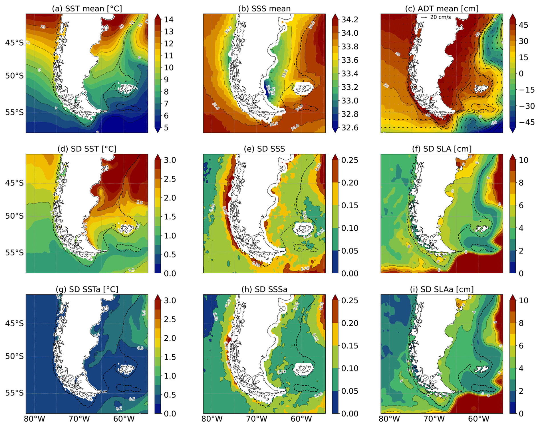
Figure 2 Mean fields of SST (a), SSS (b), and ADT (c) and their standard deviations. Panels (d), (e) and (f) show the standard deviation of the low-pass filtered time series with respect to the mean fields, thus including seasonal variability. Panels (g), (h), and (i) display the standard deviation of the anomalies after removing the annual signal. Colour intervals for the mean and standard deviations are 0.5 and 0.25 °C (SST), 0.1 and 0.05 (SSS), and 5 and 1 cm (ADT). The black arrows in panel (c) represent the mean geostrophic velocity vectors calculated from the ADT (scale shown in panel (c)). The black dashed line in all maps indicates the 200 m isobath.

4.1.1 SST

The mean SST field around southern South America exhibits a broad meridional gradient, with temperatures below 5.5 °C in the southernmost part of the domain and exceeding 14 °C around 40° S (Fig. 2a). In the Atlantic, north of ∼ 50° S, the mean SST field also exhibits a zonal gradient, characterized by differences between warmer coastal and colder offshore waters. In contrast, along the Pacific continental shelf north of 46° S, SST is lower on the shelf than in the open ocean, whereas the opposite occurs south of 46° S, where shelf waters are warmer than offshore waters. This pattern may be linked to the meridional wind divergence zone (see Fig. 3b). North of 45° S, the prevailing southerly winds induce coastal upwelling and northward flow over the shelf, favouring cooler waters near the coast. South of 45° S, the northerly winds induce downwelling and southward advection of warmer waters over the shelf.

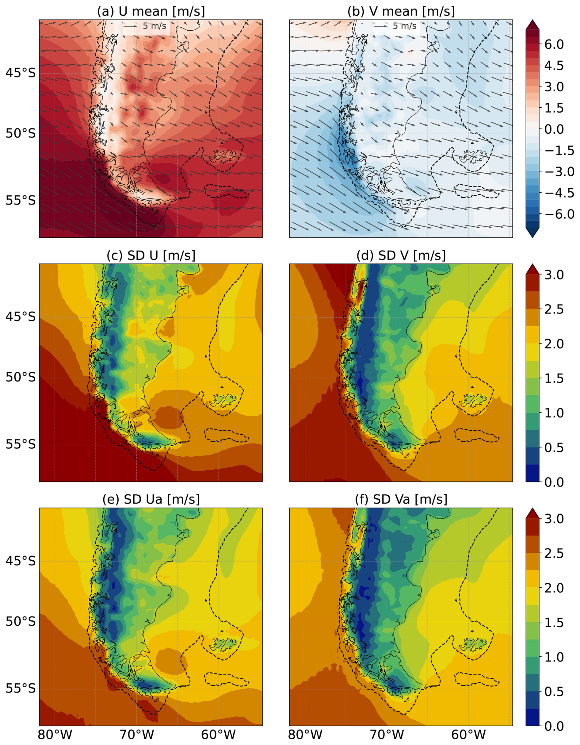
Figure 3 Mean fields of zonal ((a) m s⁻¹) and meridional wind ((b) m s⁻¹) components and their standard deviation. Panels (c) and (d) show the standard deviation of the low-pass filtered time series with respect to the mean fields, thus including seasonal variability. Panels (e) and (f) display the standard deviation of the wind anomalies, after removing the annual signal. The colour intervals are drawn every 0.5 m s⁻¹ in the mean fields and 0.25 m s⁻¹ in the standard deviation maps. The black arrows in panels (a) and (b) represent the mean wind vectors (scale shown at the top of panels). The black dashed line in all maps indicates the 200 m isobath.

On the Atlantic PCS, zonal SST gradients are much sharper in the northern sector compared to the south. SST is relatively high over the shelf but decreases sharply beyond the continental slope, where cold subantarctic waters are advected northward by the Malvinas Current (SST < 9.5 °C, Fig. 2a and c). The cold core of the Malvinas Current is located between the 200 and 2000 m isobaths, with SST increasing farther offshore. A secondary tongue of relatively cold waters is apparent over the outer continental shelf south of 47.5° S. An additional tongue of cold water extends northward to around 45° S near the Atlantic coast, likely associated with the Patagonian Current (Brandhorst and Castello, 1971; Palma and Matano, 2012). The spatial pattern of SST standard deviation (SD) in the Atlantic (Fig. 2d) displays a pronounced meridional gradient reaching values up to 4 °C, while it ranges between 1 °C and 2 °C over the Pacific shelf. It is important to note that these SD fields were computed from time series that had been previously low-pass filtered to remove high-frequency variability. Therefore, the reported values primarily reflect variability at intraseasonal to longer timescales. After removing the seasonal variability, the SD of SSTa is much smaller, typically around 0.5 °C over most of the domain, except over the northern Atlantic shelf near the continental slope where it reaches ∼ 1 °C (Fig. 2g). These patterns reflect the greater amplitude of seasonal variability, particularly in the northern part of the Atlantic domain (see Rivas, 2010).

4.1.2 SSS

Satellite-derived SSS mean values range from 32.4 to 34.7. In general, lower salinities are observed near the coast, increasing offshore (Fig. 2b). However, other notable spatial patterns emerge in the mean field. In the Pacific shelf, the lowest salinities are found along a coastal band with a minimum close to 47.5° S, consistent with previous observational studies (Dávila et al., 2002; Brun et al., 2020; Saldías et al., 2024). While satellites provide unprecedented temporal coverage, they do not provide reliable data within 40–100 km from land or within the fjords (Vinogradova et al., 2019; Jarugula et al., 2025), where salinity is known to be lower than 32 (e.g. Castillo et al., 2012; Schneider et al., 2014; Brun et al., 2020) due to significant continental freshwater input. Data availability in the Pacific portion of the PCS is limited to the Cape Horn region, where salinities are approximately 34. In the Atlantic shelf, the lowest salinity values (< 33) are observed around the eastern mouth of the Strait of Magellan, in agreement with the in-situ salinity distribution (Brun et al., 2020). However, the satellite-derived SSS does not provide data within the Strait of Magellan. Despite the limitations of satellite-derived SSS, away from the coastal band the observed pattern over the region aligns well with in-situ data from Brun et al. (2020).

The SD of SSS (Fig. 2e) exhibits increased variability near the coast, particularly along the Pacific shelf break, with values exceeding 0.4. The enhanced nearshore variability on both sides of the continent is likely associated with the combined effects of the limited resolution of satellite-borne radiometers in coastal areas and the influence of freshwater input from continental runoff. In the Pacific, significant seasonal cycles of freshwater input are associated with the melting of continental ice and substantial regional precipitation, particularly in the southeastern portion of the shelf (Dávila et al., 2002; Saldías et al., 2024). When the seasonal cycle is removed (Fig. 2h), the spatial pattern of enhanced nearshore variability persists, although overall SD values decrease. Notably, an SD maximum persists along the Pacific slope between around 47, and 51° S, where SSS SDs still exceed 0.25. This persistent variability suggests that salinity variability in this region is not only driven by seasonal forcing.

4.1.3 SLA and geostrophic velocities

The ADT mean is shown in Fig. 2c, along with the associated mean geostrophic velocities. ADT is generally higher over the Patagonian shelf than in adjacent offshore regions. A minimum in ADT is noticeable in the Antarctic Circumpolar Current in the northern Drake Passage and along the Malvinas Current. Consequently, in the Atlantic, the largest geostrophic velocities, which reach ∼ 50 cm s⁻¹, are associated with the Antarctic Circumpolar Current south of Cape Horn and the Malvinas Current near 43° S (Fig. 2c). In the Pacific sector, the Cape Horn Current exhibits moderate geostrophic velocities (∼ 30 cm s⁻¹) flowing southeastward, around Cape Horn, and toward the Atlantic.

The SD of SLA (Fig. 2f) shows a clear meridional gradient across the Atlantic shelf, with higher variability (> 6 cm) in the mid- and inner shelf north of 47.5° S. In the Pacific, no dominant pattern emerges across the entire shelf; however, somewhat higher variability is observed over the Cape Horn shelf. When the seasonal signal is removed (Fig. 2i), SD values generally decrease, as expected, yet the overall spatial structure is similar to the SD of the unfiltered data. The persistent high values over the Cape Horn shelf and along the coast of the Atlantic shelf indicate that non-seasonal processes also contribute significantly to SLAa variability over the PCS. The possible impact of non-seasonal wind variability in modulating the SLA is explored in Sect. 4.3.

4.1.4 Wind

The mean winds in the region are predominantly westerly, with lower magnitudes (∼ 5 m s⁻¹) in the northern part of the domain and exceeding 8 m s⁻¹ in the core of the westerlies south of 52° S (Fig. 3a and b).

Mean wind magnitudes are generally higher over the Pacific compared to the Atlantic, displaying a broad maximum along the Pacific coast south of 50° S and the northern Drake Passage (∼ 7 m s⁻¹). Throughout most of the domain, the mean meridional wind is northerly and weaker than the zonal wind, particularly over the Atlantic ($>-\mathrm{1.5}$ m s⁻¹), while along the Pacific coast south of 50° S it reaches ∼ −4 m s⁻¹ (Fig. 3b).

The spatial pattern of the zonal wind standard deviation (Fig. 3c) shows maximum values over the Pacific shelf south of 52° S, reaching up to 3.5 m s⁻¹ over the southern Pacific PCS. Over the Atlantic shelf, variability is lower, ranging from 1.5 to 2.8 m s⁻¹, with local maxima around 53° S. The SD of the meridional wind component (Fig. 3d) exceeds 2.5 m s⁻¹ along most of the Pacific shelf, while values over the Atlantic shelf range between 1 and 2 m s⁻¹. Although the meridional wind component is generally weak compared with the zonal component, the standard deviations are similar (Fig. 3c and d). When the seasonal cycle is removed (Figs. 3e and f), SDs decrease, but some spatial features persist. The zonal wind variability remains highest south of 52° S over the Pacific, where the strongest zonal winds are observed. Over the Atlantic shelf, it peaks at ∼ 2.5 m s⁻¹ south of 52.5° S and reaches ∼ 2 m s⁻¹ farther north. The SD of the meridional wind is fairly uniform (∼ 2–2.5 m s⁻¹) along the Pacific shelf, especially near the coast, suggesting the influence of the Andes on the local wind variability. Over the Atlantic shelf, the meridional wind variability is comparable to that of the zonal wind in most of the domain, except south of 52° S, where zonal variations are slightly stronger.

These standard deviations indicate that, over most of the domain, variations in the zonal wind component are associated with westerly winds of varying intensity. In contrast, meridional wind deviations often exceed mean values, particularly over both continental shelves, implying frequent and significant reversals in wind direction. These frequent meridional wind reversals may effectively modulate the intensity of the along-shelf circulation, with northerly winds expected to reinforce the southward mean flow over the Pacific shelf and weaken the northeastward mean flow over the Atlantic shelf (Fig. 2c), and vice versa.

4.2 Modes of variability over the Patagonian Continental Shelves

4.2.1 SSTa, SSSa and SLAa

We analysed the variability of SSTa, SSSa, and SLAa using empirical orthogonal function (EOF) analysis, focusing on the continental shelf and upper slope (depths shallower than 2800 m). The EOFs help identify the statistically dominant spatial patterns and their time variability. For clarity, hereafter we refer to the spatial patterns of each variable as EOF modes (e.g., EOF1-SSTa, EOF2-SSTa), while the associated time series are denoted as principal components (PCs; e.g., PC1-SSTa, PC2-SSTa).

EOF1-SSTa explains ∼ 54 % of the variance, displaying a monopole pattern across the PCS and adjacent slopes, with the largest variations (∼ 0.5 °C) observed near the outer shelf in the Atlantic, particularly north of 47.5° S (Fig. 4a). EOF1-SSTa also shows enhanced low-frequency variance at periods of approximately 1–4 years (Fig. 4c) and a strong intraseasonal signal between 60–150 d. Although EOF1-SSTa is significantly correlated with SSTa over most of the PCS (> 0.6), it primarily reflects variability on the Atlantic continental shelf, where correlations exceed 0.8 (see Supplement Fig. S6). EOF2-SSTa explains ∼ 11 % of the variance and displays a dipole pattern centred around 47.5° S, dividing the Atlantic PCS into two distinct regions with opposite SSTa (Fig. 4b). In contrast, the SSTa associated with EOF2 has the same sign along the western coast of South America, matching the southern part of the Atlantic dipole.

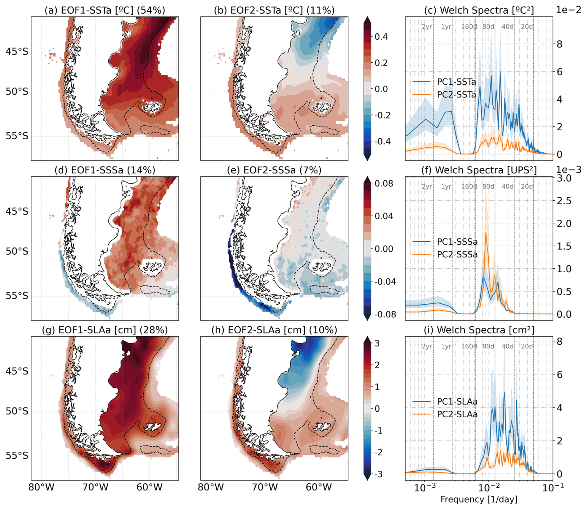
Figure 4 EOF analysis results for SSTa, SSSa, and SLAa. Panels (a) and (b) show the first and second EOF modes of SSTa, panels (d) and (e) show EOF1 and EOF2 of SSSa, and panels (g) and (h) show EOF1 and EOF2 of SLAa. Colour intervals are 0.05 °C for SSTa, 0.01 salinity units for SSSa, and 0.2 cm for SLAa. Black dashed lines in the EOF maps indicate the 200 m isobath. Panels (c), (f), and (i) display the power spectra of the corresponding PC time series for SSTa, SSSa, and SLAa, respectively, estimated using Welch's method. In the spectral plots, blue and orange curves correspond to the spectra of the first and second PCs, respectively. Spectra are shown in a variance-preserving form to emphasize the relative contribution of different frequency bands.

EOF1-SSSa explains ∼ 14 % of the total variance and exhibits a monopole over the Atlantic PCS and a dipole along the Pacific shelf break, with anomalies opposite to the Atlantic south of ∼ 50° S and of the same sign to the north (Fig. 4d). The associated temporal variability spans multiple timescales, with an apparent low-frequency contribution at periods longer than approximately 2 years as well as variability near ∼ 100 and ∼ 60 d. EOF2-SSSa accounts for ∼ 7 % of the variance and is primarily linked to intraseasonal variability, exhibiting a clear spectral peak near ∼ 100 d and meridional dipoles centred at approximately 50° S in the Atlantic and 47.5° S in the Pacific (Fig. 4e). Because SSSa variability is spatially heterogeneous and distributed across multiple modes, no single EOF captures a large fraction of the local variance; consequently, correlations between PC1-SSSa, PC2-SSSa, and the SSSa field are not statistically significant over most of the domain (see Fig. S6c and d). PC2-SSSa exhibits statistically significant correlations only in the southern Pacific PCS, along the coast, where the largest EOF2 amplitudes (exceeding 0.1) and enhanced intraseasonal variance are observed (Fig. 4e–f). Thus, despite explaining a modest portion of the total variance, EOF2-SSSa captures the most energetic intraseasonal salinity fluctuations in the southern Pacific. EOF1-SLAa explains ∼ 28 % of the total variance and displays a monopole pattern over the entire domain, with the largest variations over the Atlantic and Cape Horn shelves and somewhat smaller variations over the Pacific shelf and the southern Atlantic continental slope (Fig. 4g). Most of the variance associated with this mode lies within the 30–90 d period range (Fig. 4i). The geostrophic velocity anomalies associated with EOF1-SLAa are small, reaching ∼ 1.8 cm s⁻¹ in the Malvinas Current region and up to 2.6–3.3 cm s⁻¹ in the Cape Horn sector. Compared to the MDT, these values represent ∼ 3 % of the climatological velocities in the Malvinas region (61 cm s⁻¹), ∼ 9 % over the Cape Horn shelf (27.7 cm s⁻¹), and up to ∼ 22 % in localized regions of maximum gradients. EOF2-SLAa, explaining ∼ 10 % of the variance, displays a dipole centred north of 47.5° S on the Atlantic shelf and variability along the southern Pacific shelf of the same sign as the southern Atlantic region (Fig. 4h). The related geostrophic anomalies can reach ∼ 1.5 cm s⁻¹ in the northern Atlantic PCS. When compared to the MDT velocities in this region (2.6 cm s⁻¹), this accounts for ∼ 60 % of the mean, underscoring the regional significance of this mode despite its relatively low explained variance.

4.2.2 Wind

To analyse the wind variability, we conducted EOF analyses for the anomalies of the zonal and meridional components (Ua and Va). As with the other variables, we removed the mean, trend, high-frequency variability and seasonal cycle before the EOF analyses. The first two modes of both wind components capture approximately 77 % of the total variance, with the first mode explaining more than half of the variance in each case. Correlation maps between the PCs and the corresponding anomaly fields further show the spatial patterns associated with these modes (Fig. S7).

EOF1-Ua explains ∼ 50 % of the variance and shows a monopole with maximum variance centred around 54° S in the southern part of the domain (Fig. 5a). This centre extends zonally, with the highest intensities over the ocean near the continent, particularly in the southeast Pacific. EOF2-Ua, accounting for ∼ 27 % of the variance, displays a meridional dipole centred around 52.5° S, with greater variability at the northern and southern edges of the domain, with somewhat weaker anomalies than EOF1-Ua (Fig. 5b). The variance associated with both EOF modes is mostly centred around intraseasonal time scales, though EOF1-Ua presents more energy at 30 d, and EOF2-Ua around 60 d (Fig. 5c).

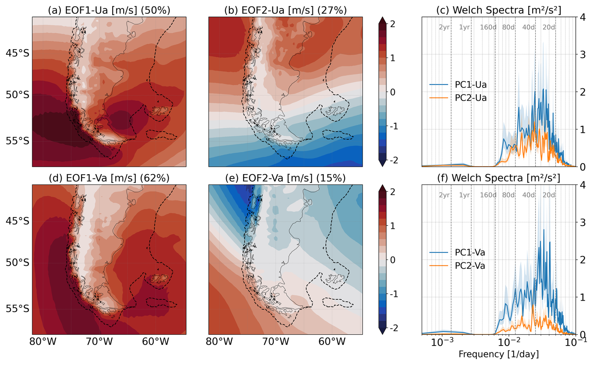
Figure 5 EOF patterns of zonal (Ua) and meridional (Va) wind anomalies. Panels (a) and (b) show EOF1 and EOF2 of zonal wind anomalies, while panels (d) and (e) show EOF1 and EOF2 of meridional wind anomalies. Colour intervals are 0.2 m s⁻¹. The black dashed line on the EOF maps indicates the 200 m isobath. Panels (c) and (f) display the power spectra of the corresponding principal component time series for zonal and meridional wind anomalies, respectively, estimated using Welch's method. In the spectral plots, blue and orange curves represent the spectra of the first and second principal components, respectively. Spectra are displayed in a variance-preserving form to highlight the distribution of variance across frequency bands.

EOF1-Va captures ∼ 62 % of the total variance, displaying a monopole with maxima in the southern Pacific region near the coast, where anomalies reach up to 1.5 m s⁻¹, and another centre near the Malvinas Islands (Fig. 5d). The variance associated with EOF1-Va is mostly intraseasonal, with the largest variance in the 30–40 d range (Fig. 5f). EOF2-Va explains ∼ 15 % of the variance, showing a meridional dipole centred around 50° S and displaying larger variations over the Pacific region (Fig. 5e).

The wind spectra show their largest peaks at periods of approximately 20–40 d, with additional but somewhat lower variability between 40 and 100 d (Fig. 5c and f). These periods overlap with the broad 30–90 d band of PC1-SLAa (Fig. 4i), associated with the monopole pattern strongest over the Atlantic and Cape Horn shelves (Fig. 4g). PC1-SSTa, which primarily represents variability over the Atlantic shelf, has enhanced variance at 60–150 d, overlapping the longer intraseasonal periods present in the wind spectra (Fig. 4a and c). The SSSa spectra show a prominent peak near 100 d, particularly in PC2-SSSa, and little variance at periods shorter than 40 d (Fig. 4f). The temporal resolution of the SSS product and its implications for this comparison are discussed in Sect. 5.2. At interannual periods, the wind PCs show comparatively little spectral energy, whereas PC1-SSTa retains low-frequency variance comparable to that observed at intraseasonal frequencies (Figs. 4c, 5c, and f). The strongest spectral overlap between the wind and ocean modes therefore occurs at intraseasonal periods. The following section examines their temporal relationships through correlations between the PCs.

4.3 Influence of wind on surface ocean variability

4.3.1 Statistical relationships between wind and ocean principal components

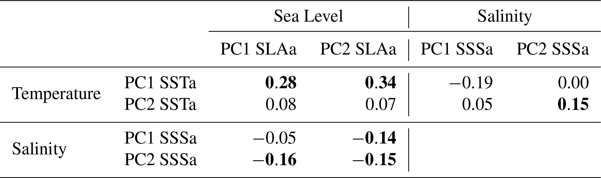
Tables 1 and 2 summarize the statistical relationships among principal components of variability in meridional and zonal wind components, temperature, salinity, and sea level. Temporal autocorrelation was accounted for when assessing correlation significance by estimating an effective sample size for each pair of time series (Sect. 3.3.3). The statistical significance of the correlations was assessed, and those significant at the 95 % confidence level are highlighted in bold (Tables 1 and 2).

Table 1 Pearson correlation coefficients between the principal components of the wind variability modes and SSTa, SSSa, and SLAa. Bold values indicate statistically significant correlations.

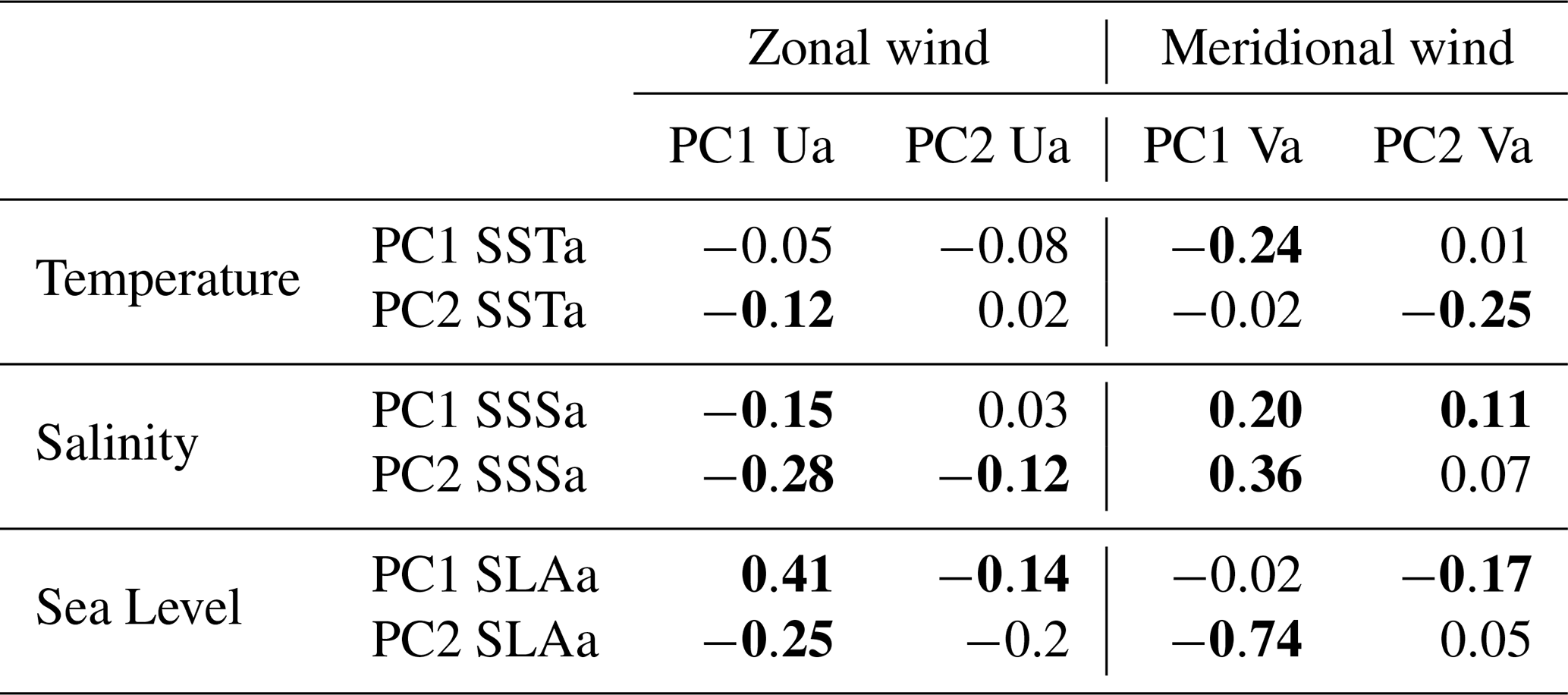
Table 2 Pearson correlation coefficients between the principal components of the variability modes of SLAa, SSTa, and SSSa. Bold values indicate statistically significant correlations.

The principal component of EOF1-Ua (PC1-Ua), which primarily represents the strengthening or weakening of the westerlies, is significantly correlated with PC1-SLAa (r=0.41), suggesting that stronger westerlies are associated with higher sea level throughout the domain. In contrast, PC1-Ua is negatively correlated with PC2-SLAa ($r=-\mathrm{0.25}$), suggesting that stronger westerlies are associated with increased SLAa over the northern Atlantic and reduced SLAa elsewhere. However, note that the anomalies linked to EOF2-SLAa are weaker, and the correlation between PC2-SLAa and the zonal wind variations is lower. PC1-Ua also shows a weaker but significant negative correlation with PC2-SSSa ($r=-\mathrm{0.28}$), pointing to a possible connection between intensified westerlies and increased coastal salinity along the southern Pacific margin.

PC1-Va, which explains 62 % of the variance in meridional winds, is weakly and negatively correlated with PC1-SSTa ($r=-\mathrm{0.24}$), indicating that enhanced southerly winds are associated with surface cooling throughout the region – particularly near the shelf break over the northern sector of the Atlantic shelf – while northerly winds are associated with surface warming. PC1-Va is further linked to salinity variability, showing positive correlations with both PC1-SSSa and PC2-SSSa (r=0.20 and r=0.36, respectively), and exhibits a strong negative correlation with PC2-SLAa ($r=-$0.74). These relationships support the hypothesis that meridional wind anomalies and the associated cross-shelf Ekman transport and induced pressure gradients modulate the along-shelf geostrophic flow and the salinity distribution. However, other patterns are not consistent. For example, the decrease in SLA over the Atlantic shelf south of 50° S is opposite to the expected response to southerly winds (see Figs. 4h and 5d), suggesting that other forcing mechanisms may control these changes.

To further investigate the possible relationship between SSTa, SSSa, and SLAa variability in Table 2, we present the correlations between their dominant principal components. PC1-SSTa is positively correlated with PC1-SLAa (r=0.28), which is consistent with a thermosteric effect. However, it also shows a somewhat higher correlation with PC2-SLAa (r=0.34), which is associated with a dipole pattern of SLAa (Fig. 4h). This is not consistent with a thermosteric response, but rather suggests that northward advection of cooler waters could drive temperature changes. In this context, SLAa gradients can induce changes in the geostrophic flow, particularly over the northern Atlantic shelf near the continental slope. Additionally, the second mode of SSSa shows weak but statistically significant negative correlations with both SLAa modes ($r=-\mathrm{0.16}$ and $r=-\mathrm{0.15}$). This mode is only relevant over the southern Pacific, where its spatial pattern significantly correlates with the observed salinity anomalies (see Fig. S6d). In this region, the inverse relationship with SLAa contrasts with the expected halosteric effect, suggesting that salinity-driven contributions to SLAa variability are minimal, despite the presence of marked salinity changes.

Altogether, these statistical relationships highlight a dynamical link between wind variability – particularly of the meridional component – and surface ocean variability over the PCS. In the following section, we use composite anomaly maps to further investigate the spatial patterns associated with the dominant modes of wind variability and to gain a deeper insight into how it modulates the circulation and water mass distribution over the PCS.

4.3.2 Composite patterns associated with wind variability

To assess the influence of wind variability on the surface properties over the PCS, we constructed composites of SSTa, SSSa, and SLAa for the positive and negative phases of the leading empirical orthogonal function modes of zonal and meridional wind variability. Phases were defined by periods during which PC1-Ua or PC1-Va exceeded ±1 standard deviation for at least five consecutive days, yielding approximately 1100 d per phase (∼ 700 d for salinity). Threshold values and annual distributions of events are provided in the supplementary material (Figs. S8 and S9). These composites describe statistical associations consistent with the proposed wind-driven mechanisms but do not establish causality on their own.

Meridional wind

EOF1 of meridional wind accounts for ∼ 62 % of the total variance and exhibits a monopolar structure centred over South America (Fig. 5d). This mode captures regional meridional wind shifts, with southerly winds prevailing during the positive phase and northerly winds during the negative phase, affecting both the Pacific and Atlantic shelves.

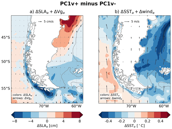
During the positive phase of meridional winds (southerly winds; Fig. 6a), widespread surface cooling is observed over both shelves, most intensely over the outer Atlantic shelf north of 50° S (∼ −0.2 °C, Fig. 6a). The opposite response occurs during the negative phase (northerly winds, ∼ 0.2 °C, Fig. 6b). While anomalies extend over the entire shelf, they are weaker over the inner shelf, particularly near San Matías Gulf and southern Grande Bay. Notably, cooling during the positive phase tends to be stronger than warming during the negative phase.

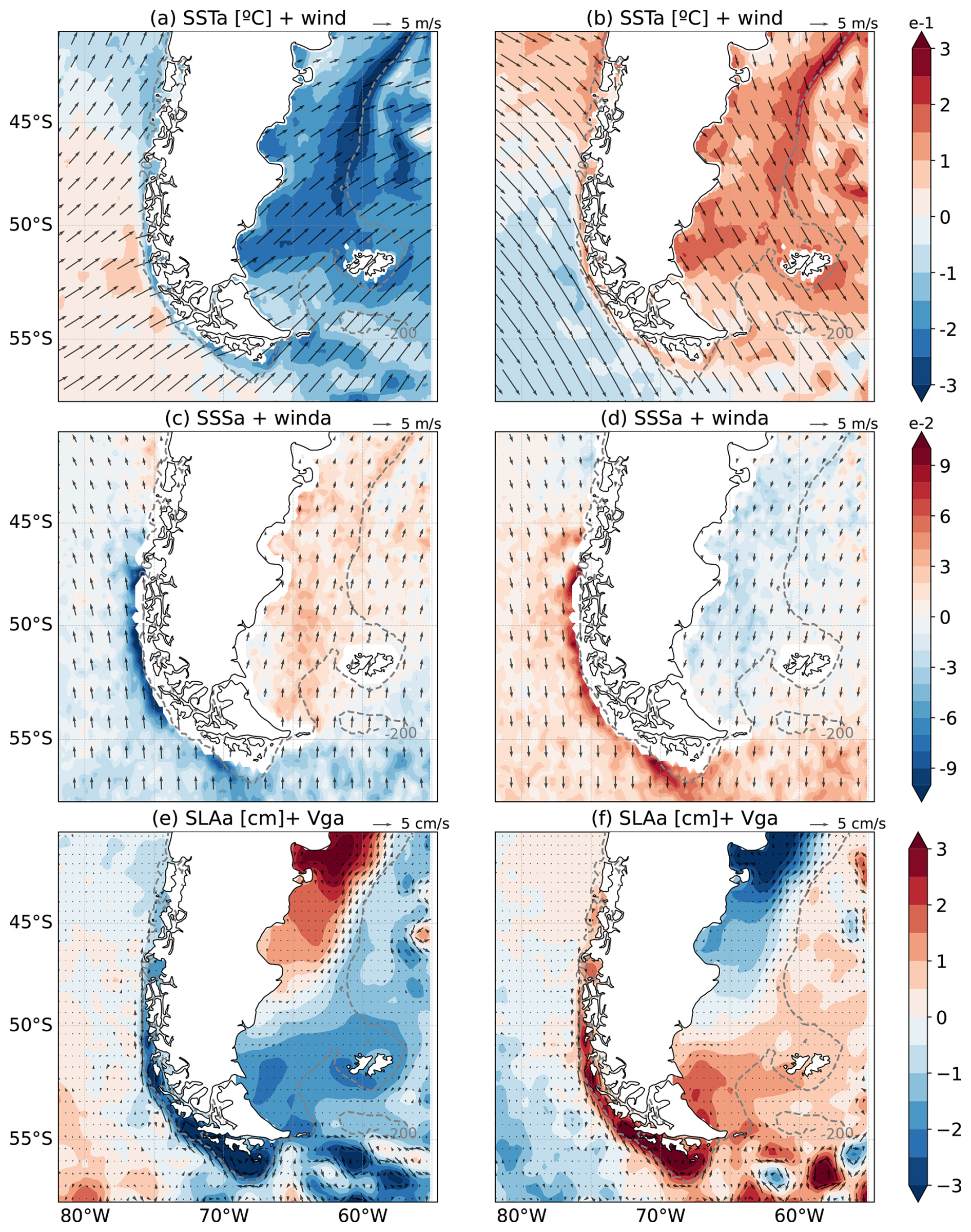
Figure 6 Composites for the positive (southerly winds) and negative (northerly winds) phases of the leading mode of the meridional wind. Panels (a), (c), and (e) show SST, SSS, and SLA anomalies for the positive phase, while panels (b), (d), and (f) show these anomalies for the negative phase. Black arrows represent wind composites in panels (a) and (b), wind anomalies in panels (c) and (d), and ocean geostrophic velocity anomalies in panels (e) and (f). Gray dashed lines indicate the 200 m isobath.

Composites of SSSa show the strongest response over the Pacific slope south of 47.5° S. During the positive phase, low-salinity anomalies exceed −0.1 (Fig. 6c). The negative phase exhibits a somewhat weaker inverse pattern (Fig. 6d). On the Atlantic shelf, southerly winds correlate with slightly saltier conditions, and northerly winds with fresher waters, although anomalies are small (< 0.05).

Under southerly winds, SLAa increases markedly over the northern Atlantic shelf, exceeding 3 cm over the mid-shelf (Fig. 6e). This sets up a zonal pressure gradient that drives northeastward geostrophic velocity anomalies of up to 2 cm s⁻¹ in the mid and outer shelf. Around 50° S, SLAa signs reverse, presenting weak and spatially diffuse anomalies over the southern Atlantic shelf, resulting in negligible geostrophic velocity anomalies (Fig. 6e). In the Pacific, SLAa patterns are more pronounced. Under southerly winds, SLAa minima form over the Cape Horn Current region, accompanied by strong horizontal gradients both offshore and nearshore. Maximum geostrophic velocity anomalies reach ∼ 5 cm s⁻¹ along the slope, suggesting a slowdown of the southward mean flow. Nearshore, the anomaly fields display patterns that resemble northward counterflows; however, these may also reflect a reduced southward transport of the Cape Horn Current, rather than a complete reversal. Given the limited accuracy of gridded altimetry maps over the coasts, the near-shore response should be interpreted with caution.

During the negative phase (northerly winds), SLAa displays a reversed pattern, forming a dipole in the Atlantic with reduced northeastward flow over the outer portion of the northern shelf, and elevated sea levels in the Pacific shelf, mostly south of 50° S and near Cape Horn, strengthening the Cape Horn Current (Fig. 6f).

Overall, SSTa, SSSa, and SLAa composites display spatially coherent responses to meridional wind variability. Anomalies consistently reverse sign between phases, and spatial patterns remain robust across different phase definitions. These structures are also supported by pointwise correlations between meridional wind and surface ocean anomalies (Fig. S10d–f). However, the SSSa signals are generally quite small, except in the southern Pacific outer shelf and upper slope regions.

Zonal wind

EOF1 of zonal wind explains ∼ 50 % of the total variance and features a monopolar pattern centred over South America, with maximum anomalies near 53° S, especially over the Pacific (Fig. 5a). This mode represents variability in westerly wind strength, with stronger winds during the positive phase. Phase-averaged wind fields (arrows in Fig. 7a and b) show intensified westerlies during the positive phase, with anomalies reaching ∼ 3 m s⁻¹ near 53° S. In the phase-averaged wind fields, winds are generally stronger over the Pacific than over the Atlantic and exhibit a slight northerly component, particularly south of 45° S in the southeast Pacific. During the negative phase, westerlies weaken and are combined with northerly anomalies across most of the domain, with peak zonal anomalies of ∼ −4 m s⁻¹ in the Pacific and weaker than −1.5 m s⁻¹ in the Atlantic (Fig. 7b).

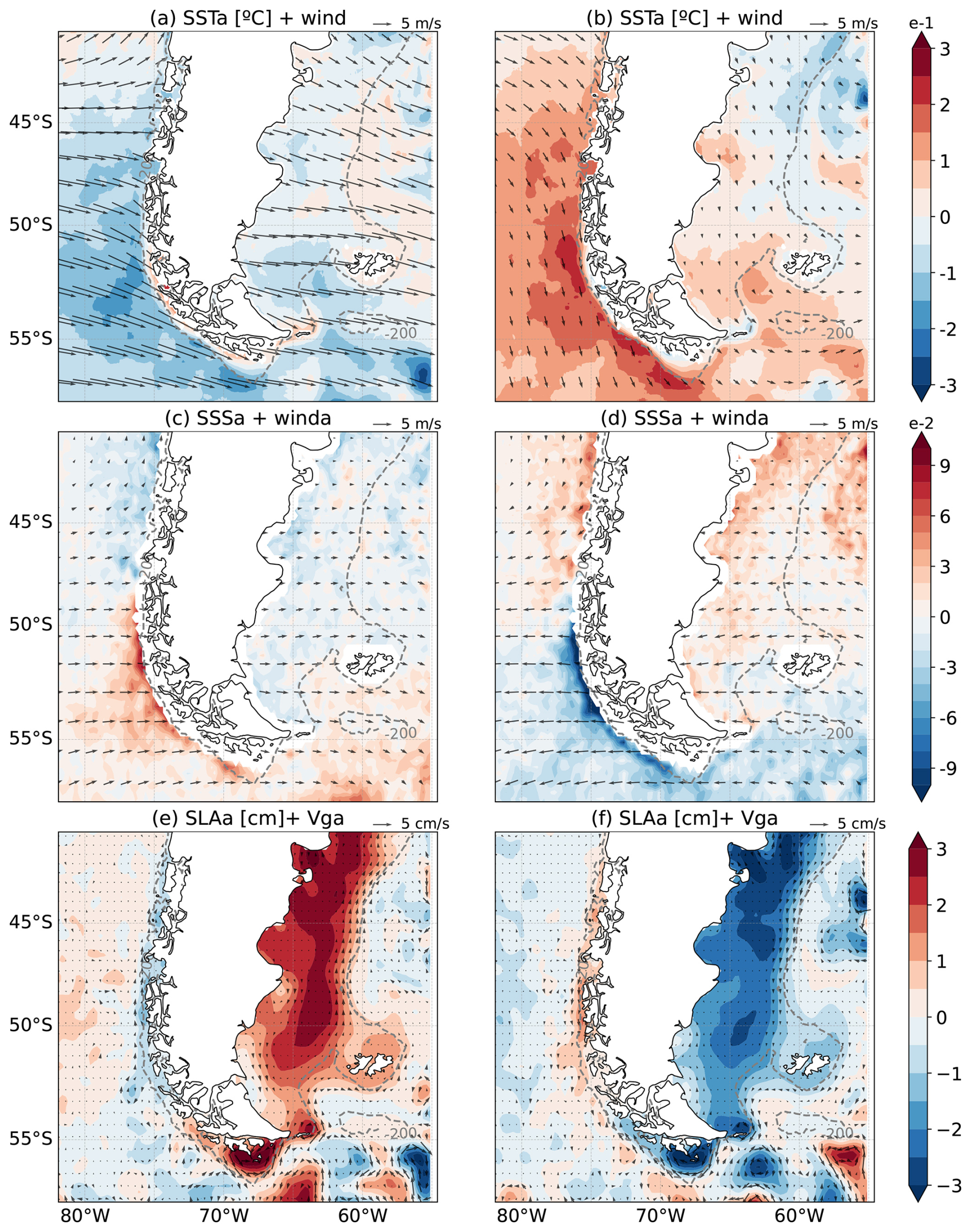
Figure 7 Composites for the positive (increased westerlies) and negative (decreased westerlies) phases of the leading mode of the zonal wind. Panels (a), (c), and (e) show SSTa, SSSa, and SLA anomalies for the positive phase, while panels (b), (d), and (f) show these anomalies for the negative phase. Black arrows represent wind composites in panels (a) and (b), wind anomalies in panels (c) and (d), and ocean geostrophic velocity anomalies in panels (e) and (f). Gray dashed lines indicate the 200 m isobath.

SSTa patterns in the PCS under zonal wind forcing are weaker compared to those associated with meridional winds (Fig. 7a and b). Intensified westerlies (positive phase, Fig. 7a) correspond to weak negative SSTa across most of the region, except in the southern Pacific PCS, where weak positive anomalies (< 1 °C) are present over the shelf south of 50° S. During the negative phase, the sign of the anomalies reverses in the Pacific; however, over the Atlantic the sign reversal is less evident, and the anomalies remain weak (< 1 °C).

SSSa composites display a clear dipole in the Pacific (Fig. 7c and d). During the positive phase, fresher anomalies occur north of ∼ 48° S and saltier anomalies to the south (Fig. 7c). This pattern reverses in the negative phase, with the strongest signals between 50–57° S along the slope. In the Atlantic, slight freshening is observed in the inner shelf during the positive phase and a weak salinity increase in the negative phase, although anomalies remain below 0.03 (Fig. 7d).

SLAa composites exhibit coherent patterns of opposite sign in each shelf. In the Atlantic, a positive SLAa monopole forms during intensified westerlies, peaking over the mid-shelf north of 52.5° S and east of Estados Island (Fig. 7e). Another variability hotspot appears over the Cape Horn shelf, with anomalies exceeding 3 cm. These regions exhibit sea level rise during the positive phase and a drop during the negative phase (Fig. 7e and f). Near the Strait of Magellan and along the coast of Grande Bay, SLAa are minimal and occasionally reverse sign compared to the neighbouring region, though uncertainties are high in this narrow, shallow and macrotidal region, where the accuracy of the altimeter retracking and of the tidal and dynamic atmospheric corrections degrades due to the proximity of the coast (Birol et al., 2025). Over the Pacific shelf north of 53° S, SLAa also reverses but is relatively small (< 1 cm), and its sign opposes that of the Atlantic and Cape Horn: sea level falls under stronger westerlies and rises when they weaken. Strongest SLAa gradients appear along the outer Atlantic shelf near the 200 m isobath (Fig. 7e and f), driving geostrophic current anomalies of ∼ 1 cm s⁻¹. These anomalies intensify the northeastward mean flow during the positive phase and reduce it during the negative phase.

5 Discussion

Our results show that wind variability plays a central role in modulating SSTa, SSSa, and SLAa across the PCS. By filtering frequencies associated with periods shorter than 20 d and removing the seasonal variability (150–400 d), we found dominant patterns in each variable that correlate significantly with the leading modes of zonal and meridional wind variability (see Table 1). These correlations, particularly those involving meridional wind, suggest that wind forcing, through both Ekman transport and geostrophic adjustment, shapes the regional circulation and water mass distribution over the shelves around southern South America.

To better understand this influence, we assessed the impact of the variability of the zonal and meridional wind components individually. We focused on how the first modes of both wind components, which explain 50 % and 62 % of the variance for the zonal and meridional components, respectively, modulate SSTa, SSSa, and SLAa. The influence of each component differs in different regions, likely due to differences in coastline orientation, morphology, and bathymetry. Winds blowing parallel to the coast generate cross-shelf pressure gradients that intensify or weaken the along-shelf geostrophic flow. Southerly winds are expected to strengthen the northward transport over the Atlantic PCS and weaken the Cape Horn Current over the Pacific, thereby altering the relative contributions of Subantarctic Water and low-salinity Pacific waters. These dynamics may also influence the exchange of water through the Strait of Magellan by modifying sea level close to the mouth on either side of the strait.

Several limitations of the datasets must be acknowledged. Land-contaminated waveforms and uncertainties in altimeter retracking, tidal corrections, and mean sea surface estimates can affect nearshore sea-level retrievals (Birol et al., 2025). Furthermore, the nominal grid spacing of interpolated altimetry products is finer than their effective resolution (Ballarotta et al., 2019). Narrow coastal structures and the geostrophic velocity anomalies inferred from SLA gradients should therefore be interpreted cautiously. Further limitations arise from the coarse temporal and spatial resolution of satellite salinity and the filtering of synoptic wind variability. While it is necessary to focus on intraseasonal to interannual scales, this filtering may lead to an underestimation of the full oceanic response to wind forcing. When high-frequency variability is retained, the standard deviation of the meridional wind is comparable to or greater than that of the zonal wind across much of the Atlantic shelf (Fig. S11), despite the predominance of westerlies in the mean field. Although the associated oceanic response lies beyond the scope of this study, this pattern suggests that synoptic-scale meridional wind variability warrants further investigation. At the other end of the frequency spectrum, the Welch segment lengths – about 5.3 years for SST, SLA, and surface winds and 3.5 years for SSS (Sect. 3.3.2) – limit the resolution of longer interannual periods. Spectral features at interannual periods should therefore be interpreted cautiously. The comparatively low wind variance at these periods does not rule out a dynamically relevant ocean response, but longer records will be required to assess this contribution more robustly. Despite these limitations, the composite analysis focuses on the most extreme wind anomalies (∼ 14 % of the time series) and similar spatial structures consistently emerge in correlation maps, reinforcing the robustness of these results (Fig. S10).

5.1 SSTa

The leading SSTa mode exhibits a monopolar structure, with a strong centre of variability over the Atlantic PCS, particularly north of ∼ 47.5° S near the slope – where the shelf widens, the bottom slope steepens, and the isobaths turn from a meridional to a northeast–southwest orientation (Fig. 4a). This mode is weakly but significantly correlated with the first mode of meridional wind variability (Fig. 5d, Table 1) and emerges prominently in the EOF1-Va composites (Fig. 6a and b). On the Atlantic shelf, these results are consistent with the hypothesis that southerly winds enhance the northward advection of relatively cold Subantarctic Shelf Water, resulting in negative SSTa. These anomalies are more intense near the Atlantic shelf break in agreement with the observations of Carranza et al. (2017), who showed that southerly winds drive onshore flow of cold Malvinas Current waters, displace the shelf break front onshore, and intensify upwelling at the shelf break. In contrast, northerly winds lead to offshore flow of relatively warm shelf waters and downwelling, which favour warming. This warming signal, however, is weaker near the shelf break compared to the cooling observed during southerly wind conditions, suggesting a stronger response under southerly phases north of 47.5° S. Another important feature of the Atlantic shelf is that the weak vertical stratification (even during summer) – largely destroyed by strong tidal mixing – along the coast implies that coastal upwelling signals in SSTa (or SSSa) are weak or absent. Indeed, climatological conditions south of 47.5° S show slightly colder surface waters nearshore compared to offshore (Fig. 2a), while subsurface waters at 50–60 m are relatively warmer than farther offshore (Romero et al., 2006).

In the Pacific coastal region, the response of SSTa to wind is consistent with upwelling/downwelling mechanisms, as suggested by Aguirre et al. (2012) at synoptic scales using numerical model simulations for central and southern Chile. Our results indicate that this mechanism may contribute at intraseasonal and interannual timescales, although the relative contribution of each band cannot be distinguished here. A contrasting response is observed between the shelf and the adjacent open ocean: while coastal regions respond primarily to wind forcing by Ekman dynamics, offshore anomalies likely reflect the influence of surface heat fluxes. This is in agreement with Aguirre et al. (2014), who noted that synoptic-scale heat fluxes play an important role in the open ocean, whereas wind-driven variability dominates near the coast.

Previous studies also provide relevant context to our results at interannual scales. SAM, which represents the dominant pattern of atmospheric variability in the Southern Hemisphere and modulates the strength and meridional fluctuations of the westerly winds, plays a key role in shaping ocean conditions over the PCS. Lovenduski and Gruber (2005) analysed the relationship between the SAM, wind speed, and SST, and found moderate negative correlations with wind speed and positive correlations with SST. An EOF analysis of SST variability during 1985–2002 in the Atlantic PCS reported a positive SAM–SSTa correlation and identified a monopolar-like pattern consistent with our findings (Rivas, 2010). Similarly, Risaro et al. (2022) analysed SST data from 1982 to 2016 over a broader domain that included open-ocean regions and found EOF patterns that resemble those presented here. These analyses suggest that the observed patterns on the PCS are robust and do not critically depend on the spatial domain or the analysis period. It is also important to note that Risaro et al. (2022) applied temporal filtering to remove variability at periods shorter than 36 months, and they further examined correlations with large-scale climate modes (Table 6 in their study). In particular, they reported significant correlations of SSTa modes with ENSO (PC2 SST) and with the Interdecadal Pacific Oscillation (PC1 and PC2 SST), highlighting the potential influence of remote climate variability on the region at interannual time scales. Remote wind forcing and large-scale climate variability were not included in our analysis and may contribute to the interannual variance of PC1-SSTa.

Overall, our results are consistent with meridional advection of Subantarctic Shelf Water being an important contributor to SSTa variability over the Atlantic shelf, an interpretation supported at interannual scales by the analysis of Bodnariuk et al. (2021). In contrast, in the Pacific, SSTa variability appears more closely linked to wind-driven upwelling/downwelling processes. Thus, although the temperature response to meridional wind variability over the Pacific and Atlantic shelves appears to involve different mechanisms, both regions display SSTa of the same sign.

5.2 SSSa

The two leading modes of SSSa variability explain only 14 % and 7 % of the total variance, and present fairly noisy distributions (Fig. 4d and e). In addition, the SSS data span a substantially shorter period (∼ 14 years) than those of other variables. Thus, the EOF and composite analyses of SSSa should be interpreted with caution. EOF1-SSSa is characterized by a monopole over the Atlantic PCS and a dipole along the Pacific shelf break (Fig. 4d), and displays energetic intraseasonal variability and a weaker low-frequency contribution (Fig. 4f). Although PC1-SSSa is statistically significantly correlated with the leading modes of both zonal and meridional wind, the magnitudes of these correlations are weak. Moreover, pointwise correlations between PC1-SSSa and the SSSa field are statistically significant only in limited areas, primarily near the Malvinas Current north of ∼ 47.5° S. The second mode, in contrast, appears to be more representative of salinity variability along the Pacific shelf break and slope south of ∼ 50° S (Fig. S6d) and exhibits larger salinity anomalies (> 0.1) compared to EOF1-SSSa. This second mode exhibits its strongest correlation with the leading mode of meridional wind (Table 1). Although the correlations remain modest in magnitude, the spatial consistency between EOF2-SSSa and the wind composites (Figs. 6 and 7, panels c and d) suggests a partial wind-driven contribution to intraseasonal salinity fluctuations. Moreover, the dipole pattern displayed by EOF1-SSSa and EOF2-SSSa resembles the first EOF mode of SSS identified by Saldías et al. (2024) in the Pacific, which they interpret as a primarily seasonal signal. In our analysis, however, the seasonal variability has been removed, suggesting that the dipole structure also reflects intraseasonal and possibly interannual processes, some of which may be associated with wind variability. It is important to note that satellite SSS observations do not capture variability at periods shorter than ∼ 40 d (Fig. 4f), and display most of the variance concentrated between 60 and 160 d. In contrast, wind variability is dominated by fluctuations between 20 and 40 d. When wind data are low-pass filtered using a 40 d cutoff, the correlations between PC2-SSSa and PC1-Ua and PC1-Va increase to 0.36 and 0.55, respectively, further suggesting the wind variability impact on SSSa at intraseasonal time scales.

The most intense SSSa during periods of strong zonal and meridional wind anomalies are observed in the Pacific PCS (panels (c) and (d) in Figs. 6 and 7, respectively). One possible explanation for this SSSa pattern is that, in the Pacific, southerly winds lead to offshore Ekman transport advecting low-salinity water from the western Patagonian fjords, resulting in negative SSSa over the continental slope. The opposite pattern – inducing positive SSSa – is observed under northerly winds. A similar modulation appears south of 48° S during periods of anomalously strong and weak zonal wind (Fig. 7c and d); however, the driving mechanism in this case remains unclear. North of 48° S, the composites of wind and SSS anomalies based on the phases of EOF1-Va show a positive meridional component (southerly) during the positive phase, corresponding to positive SSSa, and the opposite for the negative phase (Fig. 6c and d). In the composites based on the phases of EOF1-Ua (Fig. 7c and d), the zonal wind anomalies include a small meridional component, but the SSSa response does not match that observed in the Va-based composites. This indicates that SSSa variations in this region cannot be explained solely by meridional wind anomalies.

Although south of 45° S the continental runoff along the Atlantic coast is small (< 1800 m³ s⁻¹, Brun et al., 2020), variations in the substantial freshwater input from precipitation and continental runoff may strongly modulate the salinity variability off the southern coast of Chile (e.g. Dávila et al., 2002; Saldías et al., 2024). The separate contributions of advection, mixing and freshwater inputs were not quantified in this study.

Over the Atlantic shelf, SSSa patterns in the composites of EOF1-V generally show opposite signs in the two phases (Fig. 6c and d). Prevailing southerly winds are expected to reduce the southward flow in the Pacific PCS and increase the flow in the Atlantic PCS. Reduction of low salinity inflow and an increased contribution of the relatively salty subantarctic waters should therefore lead to positive SSS anomalies in the Atlantic. Conversely, under northerly wind anomalies, the inflow of Pacific waters increases, leading to negative SSSa across much of the Atlantic shelf (Fig. 6c and d), though the anomalies are weak and spatially patchy, the sign of the anomalies observed in the meridional wind composites is consistent with these changes. Southerly winds are also expected to decrease sea level along the Pacific coast and increase it over the Atlantic. Such changes would modulate the flow from the Pacific to the Atlantic through the Strait of Magellan (Guihou et al., 2020). Since the strait is the main route for lowest salinity waters entering the Atlantic PCS (Brun et al., 2020), southerly winds are also expected to lead to a salinity increase in the Atlantic. Interestingly, however, the composites constructed do not show a clear signal near the strait (Fig. 6c and d). It is important to highlight, that satellite-derived salinity products have significant limitations near the coast, often leading to gaps, interpolations, and relatively large uncertainties compared to the open ocean. As a result, SSSa observed near the Strait of Magellan should be interpreted with caution and confirmed with in-situ observations.

5.3 SLAa and associated geostrophic velocities

The leading modes of SLAa variability over the PCS (Fig. 4g and h) appear to be influenced by both zonal and meridional wind components. A quantitative comparison with MDT-derived velocities highlights the dynamical relevance of these modes. EOF1-SLAa generates relatively weak anomalies in the Malvinas Current region (∼ 1.8 cm s⁻¹, about 3 % of the climatological velocity), and stronger signals near Cape Horn, where anomalies reach up to ∼ 3.3 cm s⁻¹, representing ∼ 22 % of the local MDT-derived geostrophic velocity. In contrast, EOF2-SLAa, though explaining only 10 % of the variance, produces anomalies of ∼ 1.5 cm s⁻¹ in the northern Atlantic shelf, accounting for nearly 60 % of the mean flow, underscoring its significance despite its lower variance. These results indicate that lower-order SLAa modes can exert strong regional impacts depending on the background circulation. Specifically, the first mode of zonal wind is significantly correlated with the first and second modes of SLAa (r=0.41 and −0.25, respectively, Table 1), while the first mode of the meridional wind shows a strong negative correlation with PC2-SLAa ($r=-\mathrm{0}$.74). This agrees with the findings of Juhl et al. (2024), who associated the alongshore wind stress – significantly coherent with SLA variability at sub annual scales – with the second SLA mode. The first two EOF modes of SLAa variability over the South Atlantic shelf in a regional numerical simulation present a monopole and a dipole pattern similar to our EOF1-SLAa and EOF2-SLAa (Combes and Matano, 2018, 2019). Combes and Matano (2019) showed that the leading SLAa mode over the South Atlantic shelf – a monopole with weak spatial gradients and therefore little dynamical signature – is modulated by the combined influence of wind forcing off southern Chile and the propagation of SLAa signals from the equatorial Pacific along the South American coast. Their EOF analysis was based on SLA anomalies obtained after removing the seasonal cycle and applying a low-pass filter that retained periods longer than 60 d. Their wavelet analysis showed that the relationships of this mode with wind forcing off southern Chile and with equatorial Pacific SLA variability were particularly evident at periods longer than two years. Combes and Matano (2018) linked the second SLAa mode over the southern Atlantic shelf to the dominant mode of shelf circulation, which was primarily associated with local wind stress; they also found that relationships between shelf transport and SAM strengthened at low frequencies. This suggests a dynamic connection between the southeast Pacific and the southwest Atlantic shelves likely mediated by the Cape Horn Current and the wind systems around southern South America. Other recent studies further support this Pacific–Atlantic connection by showing that coastal trapped waves play a key role in transmitting sea-level anomalies and circulation changes along the South American margin. Synoptic disturbances reaching the PCS from the southeast Pacific act as Kelvin-like signals forced by atmospheric variability (Dinápoli and Simionato, 2025a), while lower-frequency trapped waves (40–130 d) propagate around South America and modulate the coastal current system (Poli et al., 2022). Poli et al. (2022) showed that these waves are primarily forced remotely through equatorial Kelvin waves and MJO-driven atmospheric teleconnections, and their activity strengthens during El Niño events.

The composite analysis during periods of relatively large wind anomalies further highlights the relationships between wind and SLAa variability. The wind curl was analysed in the composites of both meridional and zonal wind anomalies, and the results indicate that wind curl does not control the SLAa anomalies. It may exert some attenuation/intensification effect, but it does not explain the spatial patterns observed (not shown). The distribution of SLAa during periods when the leading mode of meridional wind exceeds one standard deviation resembles the spatial structure of EOF2-SLAa (Fig. 6e and f), while those associated with large zonal wind anomalies display a pattern that partially resembles EOF1-SLAa, but with opposite anomalies between the Pacific and Atlantic shelves (Fig. 7e and f), a feature not captured by EOF1-SLAa itself. This suggests that the zonal wind combines aspects of both EOF1 and EOF2 of SLAa. These results confirm that wind variability projects distinctly onto SLAa patterns over both the Atlantic and Pacific shelves.

Consistent with this EOF-based interpretation, SLAa in the large meridional wind anomaly composites (Fig. 6e and f) closely resembles EOF2-SLAa, as expected from its strong link to meridional wind variability, as indicated by the significant correlation between PC2-SLAa and PC1-Va ($r=-\mathrm{0}$.74; Table 1). In the South Atlantic, a dipolar structure north of ∼ 50° S indicates enhanced northward geostrophic flow during southerly wind phases (Fig. 6e), whereas south of 50° S, persistent negative SLAa under strong southerly winds suggests the influence of additional, possibly non-local, processes. An exploratory analysis of outputs of the GLORYS12 reanalysis (Lellouche et al., 2021), which provides sea surface height anomalies at $\mathrm{1}/\mathrm{12}$° × $\mathrm{1}/\mathrm{12}$° resolution, displays increased surface height along a narrow coastal band in response to southerly winds (Fig. S12). These results suggest that sea level variations along the coast of the southern Atlantic PCS may not be fully captured by the altimetry data.

High-resolution regional simulations forced by climatological winds may help understand the mechanisms driving the sea level response to meridional wind variations (Palma et al., 2004a, b, 2008). The ECMWF wind climatology used to force these simulations displays southerly winds throughout the southern Atlantic PCS (Palma et al., 2004b). Though southerly winds would act to increase coastal sea level through Ekman dynamics, south of 49° S the model presents a sharp coastal sea level depression, associated with the intense westerly winds (Palma et al., 2004a). In contrast, in that region, we find a relatively weak near-shore sea level response to anomalously strong and weak zonal winds (Fig. 7e and f).

A prominent feature shared by the EOF2 patterns of SSTa, SSSa, and SLAa is a nodal line around 47.5–50° S. This feature is also evident in the SSSa composites for both positive and negative phases of PC1-Ua and PC1-Va, and in the SLA composites for PC1-V, suggesting a possible dynamical transition zone between two regimes. At these latitudes, the Atlantic shelf undergoes marked changes in bathymetry, shelf width, and isobath orientation, while in the Pacific there is a shift in the predominant meridional wind forcing (Fig. 1, see 100 m isobath; Fig. 2). Similar transitions have been reported in previous studies near 50° S, yet the underlying mechanisms remain poorly understood.

6 Conclusions

Our results suggest that meridional wind variability plays a central role in modulating along-shelf circulation, acting asymmetrically on the Pacific and Atlantic margins. Southerly wind anomalies weaken the southward Cape Horn Current while enhancing northward flow over the Atlantic shelf – particularly on the mid/outer shelf north of ∼ 47.5° S and possibly on the inner shelf south of 47.5° S – consistent with the observed SST cooling, SSS increase, and SLA dipole patterns. Reduced inflow from the Cape Horn Current, combined with enhanced Atlantic shelf flow under southerly anomalies, implies a greater contribution of relatively salty Subantarctic Water. Similar conclusions were drawn from numerical simulations by Guihou et al. (2020), who quantified inter-ocean volume transports at interannual scales and showed that the variability of shelf exchanges around southern South America is strongly modulated by wind variability, particularly through modulation by the SAM. Our findings show that surface temperature, salinity, and sea level respond coherently to meridional wind changes, underscoring the importance of wind-driven inter-ocean exchanges in shaping the hydrographic balance of the Patagonian shelves. Our analysis shows that zonal wind variability also leads to geostrophic flow anomalies of comparable magnitude. This indicates that zonal winds may modulate shelf circulation through mechanisms that remain unclear. Further investigation, combining high-resolution models and more observations, is needed to disentangle these processes and better constrain their contribution relative to the dominant meridional wind forcing.

Overall, our findings highlight the central role of wind variability – particularly meridional winds – in shaping surface ocean variability across the Patagonian shelf system. Surface temperature, salinity, and sea level anomalies display spatially coherent and physically consistent patterns in response to wind variations, in agreement with dominant EOF modes. These results support the proposed role of wind-driven coupling between the Pacific and Atlantic shelves in modulating regional circulation and water mass distribution. The wind-driven modulation of Pacific–Atlantic transports has implications for the salinity balance, the hydrographic properties, and potentially the ecosystems of the Patagonian shelf system. Understanding these processes is crucial to anticipate future changes under climate variability and long-term trends. Addressing this challenge will require improved high-resolution regional models capable of resolving narrow straits and slope dynamics, along with an expanded network of sustained in-situ observations to better constrain and validate simulations.