Quantitative evaluation of mesoscale eddies in the North Atlantic using satellite altimetry and ocean reanalyses

Ocean mesoscale eddies (10–250 km) play a key role in transporting heat, momentum, and nutrients. Accurately evaluating their representation in ocean reanalysis becomes important given that ocean reanalysis is widely used in ocean and climate research due to their temporal and spatially consistent coverage. This study aims to assess two global ocean reanalysis products GLORYS12V1 ($\mathrm{1}/\mathrm{12}$° resolution) and GLORYS2V4 ($\mathrm{1}/\mathrm{4}$° resolution) available from the Copernicus Marine Service against satellite altimetry observations. We have used both AVISO DUACS ($\mathrm{1}/\mathrm{8}$°) and SWOT MIOST Science product ($\mathrm{1}/\mathrm{8}$°), as reference datasets that allow us to understand better the advantage of high-resolution altimetry data and have a fair evaluation for eddy-resolving ocean reanalysis ($\mathrm{1}/\mathrm{12}$°). The evaluation approach is based on a feature-based eddy-verification method to compare eddy properties, such as amplitude, radius, and centroid position, using a cost-function metric. Probability of Detection (POD) and False Alarm Ratio (FAR) are then used to quantify the reanalysis skill. GLORYS12V1 demonstrates better agreement with observations than GLORYS2V4, especially for eddies with amplitudes > 10 cm. For both AVISO DUACS $\mathrm{1}/\mathrm{8}$° and SWOT MIOST Science, the POD increases by more than 30 % when moving from GLORYS2V4 to GLORYS12V1, while the FAR increases by approximately 22 %–26 %, mainly due to the detection of more small eddies. For matched eddies, GLORYS12V1 shows a lower matching cost than GLORYS2V4 for both satellite products, with reductions of approximately 26 %. The mean errors in amplitude, radius, and centroid distance are reduced by approximately 35 %, 32 %, and 13 %, respectively. GLORYS12V1 achieves POD values of about 62 % with both references, compared with about 46 % for GLORYS2V4. FAR ranges from approximately 18 % for GLORYS2V4 to 24 % for GLORYS12V1. The results underline the added value of high model resolution for the representation of mesoscale eddies in ocean reanalyses and highlight the value of wide-swath altimetry for model verification in regions such as the North Atlantic.

1 Introduction

Ocean mesoscale features with spatial scales from tens to hundreds of kilometers and time scales from weeks to months were first observed in the early 1930s by Columbus Iselin and colleagues during Montauk-to-Bermuda Cruises, as in Cullen (2005). Since 1992, the launch of satellite altimetry missions has enabled global, high-resolution monitoring of sea level and ocean currents, significantly improving our understanding of ocean features, particularly mesoscale dynamics, as in Le Traon and Morrow (2001). Mesoscale eddies transport water masses and redistribute heat, salt, nutrients, and other tracers over large distances, and they can modulate near-surface chlorophyll (Zhang et al., 2014; Abernathey and Haller, 2018; Rhines and Young, 1982; Richardson, 1983; Chenillat et al., 2016; Yang et al., 2022; Chelton et al., 2011a). Recognizing their important role, several studies in recent years have investigated the predictability of eddies (Leroux et al., 2022; Xu et al., 2018; Thoppil et al., 2021).

Mesoscale ocean eddies can also affect tropical-cyclone intensity through warm-core ocean–atmosphere interactions (Wu et al., 2007; Wang et al., 2018). However, satellite altimetry only measures the surface signature of the eddy features. In contrast, ocean reanalyses produced by combining numerical models with observations through data assimilation schemes provide the evolution of four-dimensional ocean state estimates, enabling us to study the ocean mesoscale eddy structures not only at the surface but also in the subsurface (Lellouche et al., 2013, 2018, 2021; Martin et al., 2025). Therefore, it is important to evaluate how well ocean reanalyses represent mesoscale eddies to better understand the uncertainty inherent in these products. In recent years, the spatial resolution of ocean models has increased, allowing better representation of smaller ocean features. The first aim of this study is to evaluate the ability of ocean reanalyses with different spatial resolutions ($\mathrm{1}/\mathrm{4}$ and $\mathrm{1}/\mathrm{12}$°) to represent mesoscale eddies in the North Atlantic. Second, we assess how the verification results change when using two different satellite reference products, AVISO DUACS $\mathrm{1}/\mathrm{8}$° and SWOT MIOST Science, in order to understand whether the additional fine-scale information from SWOT modifies the evaluation of reanalysis performance.

Several studies have investigated mesoscale eddy properties, such as population, duration, lifetime, and trajectories, in satellite observations, numerical models and reanalyses (Sangrà et al., 2009; de Vos et al., 2018; Mason et al., 2019; Xie et al., 2020; Bonaduce et al., 2021; Smith and Fortin, 2022). Methods based on dynamical systems theory have also been used to track eddies (Conti et al., 2016). Eddy detection methods commonly used in these studies include approaches based on the Okubo-Weiss parameter, wavelet analysis of the relative vorticity field, and the geometry of streamlines (Souza et al., 2011). Another widely used approach, introduced by Chelton et al. (2011b), relies on satellite-altimetry fields to identify coherent eddy structures. The py-eddy-tracker package, developed by Mason et al. (2014), is also widely used to detect and track eddies at regional and global scales (Mason et al., 2017, 2019; de Vos et al., 2018; López-Álzate et al., 2022; Pegliasco et al., 2022). In the present study, we use py-eddy-tracker to perform the eddy detection and tracking process. This step is applied independently to each dataset and provides the eddy catalogues, including eddy position, amplitude, radius, polarity, and trajectories. However, evaluating the skill of an ocean reanalysis requires an additional step beyond detecting and tracking eddies independently in each dataset. Comparable object-based detection and verification problems are also encountered in atmospheric-vortex applications, including tropical-cyclone identification (Walsh, 1997; Zadra et al., 2014). In particular, it is necessary to determine whether an eddy detected in a reanalysis corresponds to the same eddy observed in satellite altimetry at a given time and location (a feature-matching and verification problem). To fill the gap, Smith and Fortin (2022) developed a verification method to evaluate the capability of ocean reanalyses in representing the eddy features at exact locations and time detected in satellite altimetry data. In this study we will adopt this method to evaluate the representation of eddies in two ocean reanalyses, thereby opening the door to a greater exploitation of ocean reanalyses. This study contributes to the Marine Environment Reanalyses Evaluation Project (MER-EP) as a case study of the initiative (Yang et al., 2025, 2026).

A reference dataset is needed to validate and evaluate the performance of ocean numerical models in representing mesoscale eddies, also as done in previous feature-based eddy verification studies (Smith and Fortin, 2022). The finer spatial resolution of ocean reanalyses creates a problem when using the AVISO DUACS $\mathrm{1}/\mathrm{4}$° dataset as a reference, because this dataset cannot capture many small-scale features. Amores et al. (2018) show that signals smaller than about 50 km can be aliased into longer wavelengths in satellite altimetry. Ballarotta et al. (2019) also showed that the effective resolution of AVISO DUACS gridded altimetry maps is lower than their nominal grid spacing. This means that some of the small-scale variability found in high-resolution reanalyses may not be shown correctly in the AVISO DUACS product. For this reason, we did not use the $\mathrm{1}/\mathrm{4}$° AVISO DUACS product in this study. Instead, we used the AVISO DUACS dataset at $\mathrm{1}/\mathrm{8}$°, which provides a finer nominal grid spacing and is consistent with the $\mathrm{1}/\mathrm{8}$° grid of the SWOT MIOST product. Its use reduces the nominal grid-spacing mismatch with GLORYS12V1, but it does not overcome the effective-resolution limits of mapped altimetry, which depends on satellite sampling and the mapping procedure rather than on grid spacing alone. Small eddies close to the resolving capability of AVISO DUACS $\mathrm{1}/\mathrm{8}$° are therefore interpreted with caution (Ubelmann et al., 2016; Amores et al., 2018; Ballarotta et al., 2019).

The AVISO DUACS $\mathrm{1}/\mathrm{8}$° satellite altimetry dataset, available from 1993 to the present at the global scale, has been widely used as a benchmark to validate and assess numerical models, ocean reanalyses, mesoscale eddy properties in many studies (Taburet et al., 2019; Mason et al., 2019; Xie et al., 2020). In this study, however, we use AVISO DUACS $\mathrm{1}/\mathrm{8}$° only over the period overlapping with SWOT MIOST Science, from 1 August 2023 to 1 May 2025, in order to apply the same verification framework to both satellite reference products.

The availability of observations from the SWOT (Surface Water and Ocean Topography) wide-swath satellite altimetry mission provides another possible reference dataset for evaluating the capability of higher-resolution ocean reanalyses to identify and track mesoscale eddies over time in a regional domain. SWOT was launched in December 2022 (EO Portal, 2024) and offers wide-swath measurements of sea surface height, which allows observations of ocean features at much finer spatial scales than traditional altimetry (Fu and Ubelmann, 2014). One of the objectives of SWOT is the observation of two-dimensional ocean surface topography and the characterization of mesoscale and submesoscale ocean circulation (SWOT Science Team, 2024). Nevertheless, one important application of SWOT observations is their use in ocean analysis and forecasting systems through data assimilation, since wide-swath SSH observations can help better constrain mesoscale features and smaller-scale variability (Morrow et al., 2019; Fouchet et al., 2025). In the present study, however, we do not use the native SWOT swath observations directly. We use the experimental SWOT MIOST Science product, a global daily Level-4 gridded reconstruction of sea-surface height and derived geostrophic velocities produced by SSALTO/DUACS. MIOST stands for Multiscale Interpolation Ocean Science Topography. It merges irregularly sampled altimeter observations into fields that are continuous in space and time using a linear optimal-interpolation framework in which different covariance functions can be used to represent variability at different spatial and temporal scales. In the configuration considered here, the covariance functions are designed primarily to represent mesoscale geostrophic variability (Ubelmann et al., 2021; CLS and CNES, 2025). SWOT Level-4 sea-level products are not limited to the MIOST reconstruction used in this study. AVISO/DUACS also distributes experimental regional products generated using 4DVarNET and 4DVarQG. The 4DVarNET approach combines a variational data-assimilation formulation with a deep-learning framework to learn both the representation of ocean dynamics and the associated solver (Fablet et al., 2021; Beauchamp et al., 2023). In contrast, 4DVarQG uses a four-dimensional variational scheme constrained by a reduced-order quasi-geostrophic model, introducing an explicit dynamic prior into the reconstruction (Le Guillou et al., 2021).

Comparisons over the North Atlantic indicate that 4DVarNET and 4DVarQG are capable of providing finer effective resolution and improving the reconstruction of the energetic and nonlinear structures of the Gulf Stream compared to MIOST, although their performance may vary spatially and neither method currently provides a global mapping solution (Ballarotta et al., 2025). MIOST is selected because it provides a spatially consistent global reconstruction (such as AVISO DUACS $\mathrm{1}/\mathrm{8}$°) covering the intended validation domain, the North Atlantic, up to the upper mid-latitudes (60° N). The 4DVarNET and 4DVarQG experimental maps, as of the study's final implementation (October and November 2025), were regional products covering approximately 25–50° N and 80–10° W and therefore do not include the northern part of our study region. However, there are some important limitations that must also be considered. First, because the mission is very recent, the time coverage of SWOT data is limited. Therefore, SWOT data cannot yet be used to study decadal or long-term variability of mesoscale activity. In this study, SWOT is used only for a short-period evaluation of the representation of mesoscale and smaller-scale eddy features in high-resolution reanalyses. Second, since similar nadir altimetry observations are assimilated in some ocean reanalysis products considered in this study, neither AVISO DUACS $\mathrm{1}/\mathrm{8}$° nor SWOT MIOST Science can be regarded as a fully independent verification dataset. DUACS $\mathrm{1}/\mathrm{8}$° is based on multi-mission nadir altimetry, while SWOT MIOST Science combines SWOT wide-swath observations with a multi-mission nadir-altimetry background used to constrain the larger-scale signal. Therefore, both satellite products share, at least partly, observational information with the reanalyses. However, SWOT MIOST Science also introduces additional fine-scale information from SWOT wide-swath measurements, which is not directly assimilated in the reanalysis products considered here. For these reasons, AVISO DUACS $\mathrm{1}/\mathrm{8}$° and SWOT MIOST Science are used as complementary evaluation references rather than as absolute observational truth. The comparison with SWOT provides insight into how well the reanalyses represent fine-scale variability revealed by wide-swath altimetry, whereas the DUACS comparison provides continuity with the longer pre-SWOT altimetry record.

This complementary approach allows us to assess the representation of mesoscale eddies in the reanalyses while explicitly acknowledging the limitations associated with the partial dependence of the reference datasets.

An evaluation over the full period of the reanalyses era (1993–present), including the uncertainties associated with altimetry constellation and mapping procedures, will be left for a future study.

The paper is organized as follows. Section 2 describes the datasets and methods, Sect. 3 presents the verification results, and Sect. 4 summarizes and discusses the main findings.

2 Data and methods

In this study, we use two Global Ocean Reanalysis datasets, GLORYS12V1 and GLORYS2V4, and two standard satellite-altimetry gridded-observational products, AVISO DUACS L4 product and SWOT MIOST L4 product. Detailed descriptions are provided below.

2.1 Satellite altimetry products

The AVISO DUACS global $\mathrm{1}/\mathrm{8}$° daily gridded product provides sea level anomaly (SLA), absolute dynamic topography (ADT), and geostrophic velocities derived from multi-mission satellite altimetry. The product is generated by the CNES/CLS DUACS system and distributed by the Copernicus Marine Service (Copernicus Marine Service, 2025a; Taburet et al., 2019; Ballarotta et al., 2019). Although its nominal grid spacing is $\mathrm{1}/\mathrm{8}$° (approximately 12.5 km), its effective resolution is lower because the optimal-interpolation procedure smooths part of the small-scale variability. Its effective resolving capability is typically between 50 and 100 km, depending on latitude and the observing constellation, which limits the representation of the smallest mesoscale and submesoscale features (Chelton et al., 2011b; Ballarotta et al., 2019; Copernicus Marine Service, 2025a, b).

To complement the standard DUACS product, we also use the experimental global $\mathrm{1}/\mathrm{8}$° SWOT MIOST Science gridded sea-level dataset distributed by AVISO/DUACS (CLS and CNES, 2025). This product combines multi-mission nadir altimetry with SWOT observations and uses the MIOST framework to reconstruct fields that are continuous in space and time through a multiscale optimal-interpolation approach designed to represent mesoscale geostrophic variability (Ubelmann et al., 2015; Rogé et al., 2017; CLS and CNES, 2025). However, SWOT MIOST remains a daily Level-4 mapped product and should not be interpreted as a direct representation of the native KaRIn observations. Its smallest-scale variability is still affected by observational noise, filtering, interpolation, and the spatial and temporal sampling of the observing system. In addition, its relatively short temporal coverage limits its use for investigating decadal or longer-term variability.

The SWOT Level-4 products over the North Atlantic are not limited to MIOST. As noted in the Introduction, other experimental regional products, including 4DVarNET and 4DVarQG, are also available and use different data-driven or dynamically constrained mapping approaches (Le Guillou et al., 2021; Beauchamp et al., 2023; Ballarotta et al., 2025). As explained in Introduction, we select MIOST because it provides a spatially consistent global reconstruction covering the complete verification domain, differently from these other products that don't include the whole study area.

The AVISO DUACS $\mathrm{1}/\mathrm{8}$° product used in this study corresponds to the Copernicus Marine Service product SEALEVEL_GLO_PHY_L4_MY_008_047, dataset cmems_obs-sl_glo_phy-ssh_my_allsat-l4-duacs-0.125deg_P1D, https://doi.org/10.48670/moi-00148 (CLS, 2018). This product was accessed and downloaded on 31 October 2025.

The SWOT MIOST Science product used in this study corresponds to the AVISO/DUACS Experimental Multimission Gridded Level-4 Sea Surface Heights and Velocities product including SWOT observations, generated using the MIOST mapping method, version 2.0.1, https://doi.org/10.24400/527896/A01-2025.001 (CNES and CLS, 2025). This product was accessed and downloaded from the v_2_0_1/miost/science directory on 1 November 2025.

2.2 Global ocean reanalysis products

To evaluate the impact of the spatial resolution on reanalysis skills, we used two Global Ocean Reanalysis products, distributed by CMEMS: GLORYS2V4 and GLORYS12V1. These products are part of the CMEMS multi-year reanalysis portfolio and are designed to deliver consistent, observation-constrained reconstructions of the ocean state over the satellite altimetry era (1993–present).

The product configuration and quality information are documented by the Copernicus Marine Service (Copernicus Marine Service, 2023). GLORYS12V1 is an eddy-resolving reanalysis, developed by Mercator Ocean International. It provides a global ocean reanalysis at $\mathrm{1}/\mathrm{12}$° horizontal resolution (∼ 8 km), with 50 vertical levels. The system is based on the NEMO ocean general circulation model (v3.1) coupled with the LIM2 sea-ice model and uses Arakawa C-grid discretization, as explained in Madec and the NEMO System Team (2024). The reanalysis assimilates along-track delayed-time sea-level anomaly (SLA) from all altimetric satellites, AVHRR-only Reynolds SST ($\mathrm{1}/\mathrm{4}$°), in-situ temperature and salinity profiles from the CORA v4.1 database (Cabanes et al., 2013; Szekely et al., 2019), and sea-ice concentration from CERSAT (Ezraty et al., 2007).

For both comparisons, the study requires the use of the interim extension for GLORYS12V1 (cmems_mod_glo_phy_myint_0.083deg_P1D-m), daily mean sea surface height fields from the interim archive, matching the same period used for satellite datasets.

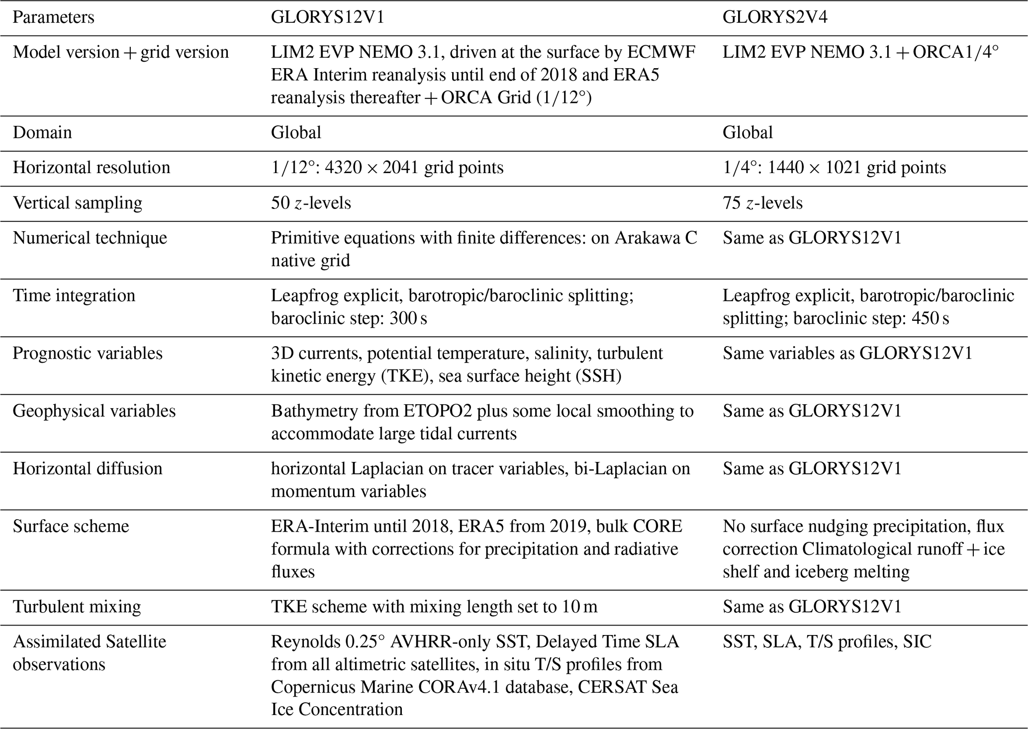
GLORYS2V4 is a lower-resolution global ocean reanalysis included in the Copernicus Marine Global Ocean Ensemble Physics Reanalysis product. It is based on the NEMO v3.1 model framework coupled with the LIM2 thermodynamic–dynamic sea ice model, configured on the ORCA025 grid (Madec and Imbard, 1996) with a nominal horizontal resolution of $\mathrm{1}/\mathrm{4}$° and 75 vertical levels. For the present study, the temporal coverage selected for GLORYS2V4 also matches the period used for the satellite datasets, in order to allow a direct comparison with GLORYS12V1. All details on the main parameters of the two reanalysis products are included in Table 1.

Table 1 Main characteristics of GLORYS12V1 and GLORYS2V4. Both reanalysis datasets use the SAM2 assimilation scheme with a large-scale bias correction, a 7 d assimilation window, and a merged model-observation mean dynamic topography (MDT). The assimilated observations are summarized below.

GLORYS12V1 was obtained from the Copernicus Marine Service product GLOBAL_MULTIYEAR_PHY_001_030, https://doi.org/10.48670/moi-00021 (Mercator Ocean International, 2023). The product was accessed and downloaded on 1 November 2025.

GLORYS2V4 was obtained from the Copernicus Marine Service product GLOBAL_MULTIYEAR_PHY_ENS_001_031, https://doi.org/10.48670/moi-00024 (Mercator Ocean International, 2024). The product was accessed and downloaded on 1 November 2025.

2.3 Verification period and domain

As mentioned in Sect. 2.2, the analysis was conducted over the period from 1 August 2023 to 1 May 2025. This period corresponds primarily to the availability of daily outputs from SWOT MIOST and both reanalysis systems, and it ensures the overlap with the DUACS $\mathrm{1}/\mathrm{8}$° observational datasets and provides a sufficient window for an eddy statistics evaluation. An evaluation of eddy statistics over the full period of the reanalysis products is left to a future study. Here, our focus is to demonstrate the robustness of the verification approach and to assess the sensitivity of the reanalysis evaluation to the choice of satellite altimetry reference product by using two different satellite datasets. Before the application of the verification method, all products are previously interpolated to a $\mathrm{1}/\mathrm{8}$° regular grid (DUACS $\mathrm{1}/\mathrm{8}$° and SWOT MIOST Science grids), and high-pass filtered using a Bessel filter with a 500 km cutoff, as described in Mason et al. (2014), to isolate the mesoscale signals (see Appendix D for more details about different spatial Bessel filter cutoff wavelength). The same parameters are also used for the eddy detection algorithm. The verification domain is defined as the region bounded by 29.8–59.8° N in latitude and 80.1–30.1° W for longitude, to include the Gulf Stream influence region, as described in Smith and Fortin (2022). This region is known for its intense mesoscale activity and high eddy kinetic energy, making it particularly suitable for validating eddy-resolving capabilities of ocean analysis and reanalysis systems.

2.4 Eddy verification methodology

The detection and tracking of mesoscale eddies in this study follow the standard procedure implemented in py-eddy-tracker, as described in Mason et al. (2014, 2019) and Pegliasco et al. (2021), and used by Smith and Fortin (2022) in their verification methodology. It is based on identifying closed contours in daily fields of Sea Level Anomaly (SLA) or Sea Surface Height (SSH), and using the associated geostrophic velocities to classify the rotation polarity. We have adopted the approach described by Pegliasco et al. (2021), where the detection is performed on SSH (or Absolute Dynamic Topography) fields rather than SLA to reduce the risk of misidentifying Gulf Stream meanders as eddies, an issue commonly encountered when using SLA in strongly sheared regions. A closed contour is “accepted” as an eddy, in other words, it is considered a “detected” eddy for py-eddy-tracker routine, if it satisfies the following criteria:

• It must contain a single maximum (for Anticyclonic) or minimum (for Cyclonic).

• The shape must be roughly circular, with a contour area not deviating more than 55 % from a perfect circle.

• The enclosed area must contain between 5 and 2000 pixels (I_min = 5 ≤ I ≤ I_max = 2000).

• The amplitude, computed as the difference between the contour extremum and the outermost valid contour, must be at least twice the contour interval. With the 0.2 cm contour interval used here, this gives a minimum algorithmic threshold of 0.4 cm. This low value is used only as a permissive detection criterion and not as a physical threshold for eddies; weak features are assessed later through lifetime filtering and amplitude-dependent verification statistics (see Sect. 3.2 and Appendix C for more details).

After the detection of eddies for each date, eddies are tracked in time using cost function C (Eq. 1), which links eddies on consecutive days based on similarity in amplitude, radius, and centroid position. For a particular eddy, all eddies within a radius of 125 km are identified. The cost function, adopted for each pair of eddies, is based on the difference in amplitude A, in effective radius R and distance D, and it is defined as:

$$\begin{array}{}\text{(1)}& C=\sqrt{{\displaystyle \frac{{\left(A_{\mathrm{1}}-A_{\mathrm{2}}\right)}^{\mathrm{2}}}{A_{\mathrm{1}}^{\mathrm{2}}}}+{\displaystyle \frac{{\left(R_{\mathrm{1}}-R_{\mathrm{2}}\right)}^{\mathrm{2}}}{R_{\mathrm{1}}^{\mathrm{2}}}}+{\displaystyle \frac{{\left(D\right)}^{\mathrm{2}}}{(\mathrm{125}\mathrm{km}{)}^{\mathrm{2}}}}}\end{array}$$

where the subscripts 1 and 2 denote, respectively, the satellite eddy and the candidate reanalysis eddy in the matching procedure. In the tracking procedure, they denote a detected eddy at time t and a candidate continuation at time t+1, respectively (see Appendix D for more details about the use of a different distance threshold of the matching cost function).

A minimum lifetime threshold is applied to reduce the identification of transient or spurious features, as in Mason et al. (2014). In this study, we adopt a 4 d minimum lifetime threshold, requiring each eddy to be detected on consecutive days without observational gaps. This relatively short threshold is used to verify the ability of the reanalyses to represent the full spectrum of mesoscale features detected in the satellite products, including short-lived eddies that may still affect the matching statistics. In addition, we have also introduced a calculation with minimum lifetime thresholds of 7 and 28 d (see Appendix A, for more details). A lifetime threshold of 7 d is also used for certain evaluations to demonstrate the sensitivity to this choice (e.g., 4 d). The 28 d threshold is useful for isolating persistent structures, but it is not our primary choice because the aim is also to evaluate the entire population, including short-lived eddies. Eddy properties such as effective radius, amplitude, trajectory, and lifetime are computed for each track. The effective radius is defined as the radius of a circle with the same area enclosed by the eddy contour.

The consistent workflow reduces processing-related differences among products, although effects associated with remapping, native resolution, effective resolution, and observational sampling remain (Droghei et al., 2018; Ciani et al., 2019, 2025). First, a spectral analysis of the four products was performed using 1 January 2025 as a representative test case. All datasets are remapped onto the same regular $\mathrm{1}/\mathrm{8}$° grid, which is the native grid of both SWOT and DUACS. Figure 1 shows the SSH fields used in this study from GLORYS12V1, GLORYS2V4, SWOT MIOST Science and AVISO DUACS $\mathrm{1}/\mathrm{8}$°. For the two reanalysis products, GLORYS12V1 and GLORYS2V4, SSH represents the modelled sea-surface height above the model geoid or reference equipotential surface, as described in Lellouche et al. (2021). For the satellite altimetry products used in this study, the corresponding SSH field is represented by Absolute Dynamic Topography (ADT), which is the sea-surface height above the geoid and is obtained by adding the Mean Dynamic Topography (MDT) to the Sea Level Anomaly (SLA) (i.e. ADT = SLA + MDT, as explained in Mulet et al., 2021). Although the reanalysis SSH and satellite ADT are not identical data products, since the former is produced by ocean models constrained by data assimilation and the latter is derived from satellite altimetry and an estimated MDT, they can be considered dynamically comparable, because they provide dynamically comparable representations of sea-surface dynamic topography, from which surface geostrophic currents are derived. As described in Mason et al. (2014, 2019) and Pegliasco et al. (2021), contour-based eddy detection and tracking methods, such as those implemented in py-eddy-tracker, can be consistently applied to both fields because they mainly rely on local extrema, closed contours, spatial gradients, and centre-to-edge height differences. The superimposition of the detected eddies on the SSH/ADT background also allows their sizes and positions to be evaluated in relation to the Gulf Stream pathway.

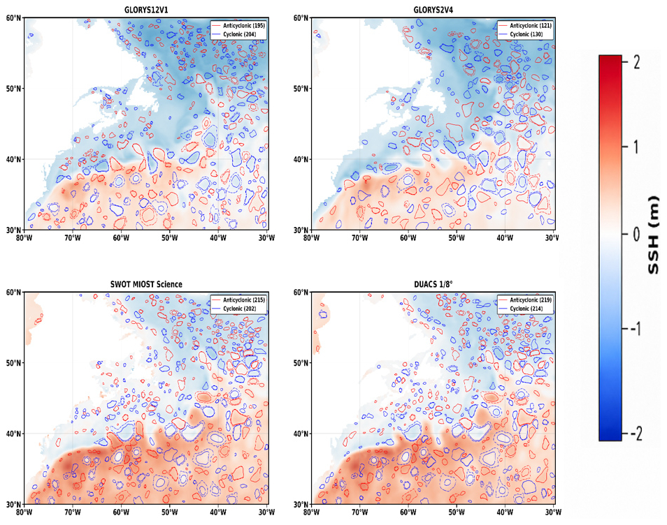
Figure 1 Daily sea-level fields on 1 January 2025 for GLORYS12V1, GLORYS2V4, SWOT MIOST Science, and AVISO DUACS $\mathrm{1}/\mathrm{8}$°, after application of a high-pass Bessel filter with a cutoff wavelength of 500 km. The common colour bar is labelled SSH (m), with SSH used here as a general label for the sea-surface height field. Specifically, the colour shading represents modelled SSH for GLORYS12V1 and GLORYS2V4 and satellite-derived Absolute Dynamic Topography (ADT) for SWOT MIOST Science and AVISO DUACS $\mathrm{1}/\mathrm{8}$°. Although SSH and ADT are not formally identical quantities, they are dynamically comparable and are treated consistently for contour-based eddy detection. Detected anticyclonic and cyclonic eddies are overlaid in red and blue, respectively. Solid contours indicate the contour of maximum circum-averaged geostrophic speed, whereas dashed contours indicate the effective contour used to calculate eddy area and effective radius. All fields were remapped onto the same regular $\mathrm{1}/\mathrm{8}$° grid to allow direct comparison.

In analogy to the approach adopted in Droghei et al. (2018) and Ciani et al. (2019), we selected the North-West Atlantic region and computed one-dimensional wavenumber spectra using a fast Fourier transform (FFT) to quantify the spatial scales effectively represented by each dataset. To avoid the latitude-dependent distortion associated with zonal wavenumbers expressed in degrees, all SSH fields were first projected onto a Lambert Azimuthal Equal-Area coordinate system centred on the study domain. The fields were then interpolated onto a regular kilometre-scale grid with dx= dy= 12.5 km. The one-dimensional zonal and meridional spectra were computed on this projected grid using FFTs. The resulting wavenumbers are therefore expressed in cycles per kilometre, with the corresponding wavelengths shown in kilometres.

Figure 2 reports the comparative spectral analysis of the four SSH fields along the zonal and meridional directions on the projected grid. At large spatial scales, approximately larger than 200 km, all spectra exhibit comparable energy levels, indicating a consistent representation of the dominant mesoscale structures. At shorter wavelengths, differences become more evident. In the meridional direction, SWOT systematically exhibits the highest spectral energy over most of the resolved range, with a clearer separation from the other products below about 100 km. DUACS and GLORYS12V1 show intermediate and broadly similar energy levels, whereas GLORYS2V4 generally displays the weakest small-scale energy. In the zonal direction, the four spectra are also similar at large scales, but a progressive separation emerges toward smaller wavelengths, with SWOT again retaining the highest spectral energy. Over much of the mesoscale range, GLORYS12V1 and DUACS remain relatively close, while GLORYS2V4 decreases more rapidly. At wavelengths shorter than about 50 km, all spectra show a marked decay, but SWOT continues to preserve the largest amount of variance, and GLORYS12V1 generally retains more small-scale zonal energy than GLORYS2V4. Overall, these spectra indicate that the SWOT product better preserves fine-scale variability, while the higher-resolution GLORYS12V1 reanalysis captures small-scale mesoscale energy more effectively than GLORYS2V4.

Figure 2 Power spectral density of SSH, corresponding to ADT for the satellite altimetry products, for the four datasets on 1 January 2025 over the selected North Atlantic region. All fields were projected onto a Lambert Azimuthal Equal-Area coordinate system and interpolated onto a regular kilometre-scale grid with $\mathrm{d}x=\mathrm{d}y=$ 12.5 km, before computing the spectra. Panel (a) shows the meridional spectrum and panel (b) the zonal spectrum. Wavenumbers are expressed in cycles per kilometre, with the corresponding wavelengths shown in kilometres on the upper x axis.

In Fig. 3, we see the dependence between radius and amplitude, in which we note that eddies display similar properties in terms of effective radius and amplitude. Many small eddies are detected with a radius below 50 km and amplitude less than 5 cm. In Fig. 4, most eddies have amplitudes lower than 10 cm. However, their mean lifetime is lower than 50 d (see Appendix C for more details about mean lifetime and eddy amplitude thresholds). However, features with amplitudes of only a few millimetres should not be interpreted as physically robust eddies. The 0.4 cm value corresponds only to the permissive algorithmic threshold used during the py-eddy-tracker detection step, and is not used here as a physical threshold to define the robust eddy population. It can be noted, generally, that larger amplitude eddies are also found to have larger radius (Fig. 3). The eddy identification and tracking procedure are independently applied for each product and produce plots about physical features and time series of anticyclonic and cyclonic eddies.

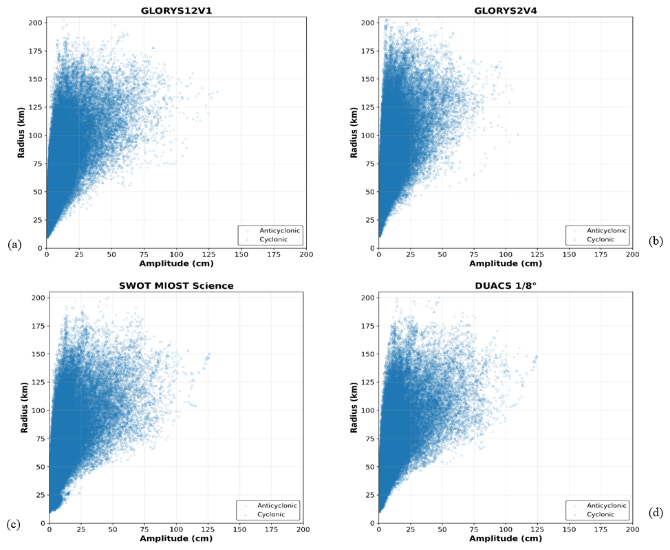
Figure 3 Scatter plots of detected eddies, with a minimum lifetime threshold of 4 d, showing the relationship between radius and eddy amplitude, from 1 August 2023 to 1 May 2025, for (a) GLORYS12V1 (bilinear remapped onto DUACS and SWOT grid), (b) GLORYS2V4 (bilinear remapped onto DUACS and SWOT grid), (c) SWOT MIOST Science, and (d) AVISO DUACS $\mathrm{1}/\mathrm{8}$°. The eddy amplitude and the eddy radius are calculated at the track level, by averaging the amplitude and radius over the entire lifetime of the eddy.

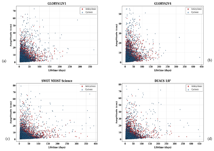
Figure 4 Scatter plots of identified eddies, with a lifetime threshold of 4 d, showing eddy amplitude versus eddy lifetime for (a) GLORYS12V1, (b) GLORYS2V4, (c) SWOT, (d) DUACS. Each eddy is counted only once. The eddy amplitude is calculated at the track level, by averaging the amplitude over the entire lifetime of the eddy.

The same cost function (1) used for the tracking procedure is also used to match the eddies between the reanalysis and the observed eddy (satellite). This function allows us to see how the eddies can be matched even if they have different values for radius, amplitude, mean centroid position. Although one or more of these parameters can vary, for an eddy to be considered matched to the corresponding satellite dataset, the cost function must be minimized, provided that the distance between the eddy centroids does not exceed 125 km (is set to 125 km, i.e., that's slightly greater than the average diameter of eddies in the North Atlantic region; see Ballarotta et al., 2019).

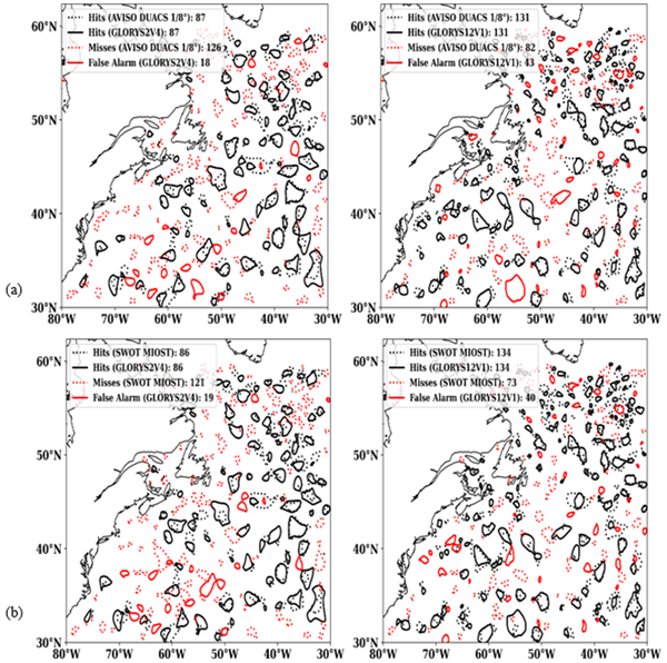
Therefore, following the application of the matching algorithm, as described in Smith and Fortin (2022), an eddy identified in both the reanalysis (i.e. GLORYS2V4 and GLORYS12V1) and verifying datasets (DUACS and SWOT products) is referred to as “hit”. An eddy in the verifying dataset with no corresponding eddy in the reanalysis is referred to as a “miss”, whereas an eddy present in a reanalysis but not in the verifying dataset, is deemed as a “false alarm”. In Fig. 5a and b, we see an example of eddy matching procedure for both comparisons, following the concept of the matching algorithm, described in Smith and Fortin (2022). The statistics for hits, misses and false alarms can be tabulated over the study area and over the full evaluation period to provide an indication of the skill of two reanalysis products in representing the “observed eddies”. It is interesting to consider what fraction of the observed eddies are captured (not excluded) by reanalysis products, using the Probability of Detection (POD), as introduced and explained in Smith and Fortin (2022), defined as:

$$\begin{array}{}\text{(2)}& \mathrm{POD}={\displaystyle \frac{\mathrm{hits}}{(\mathrm{hits}+\mathrm{misses})}}\end{array}$$

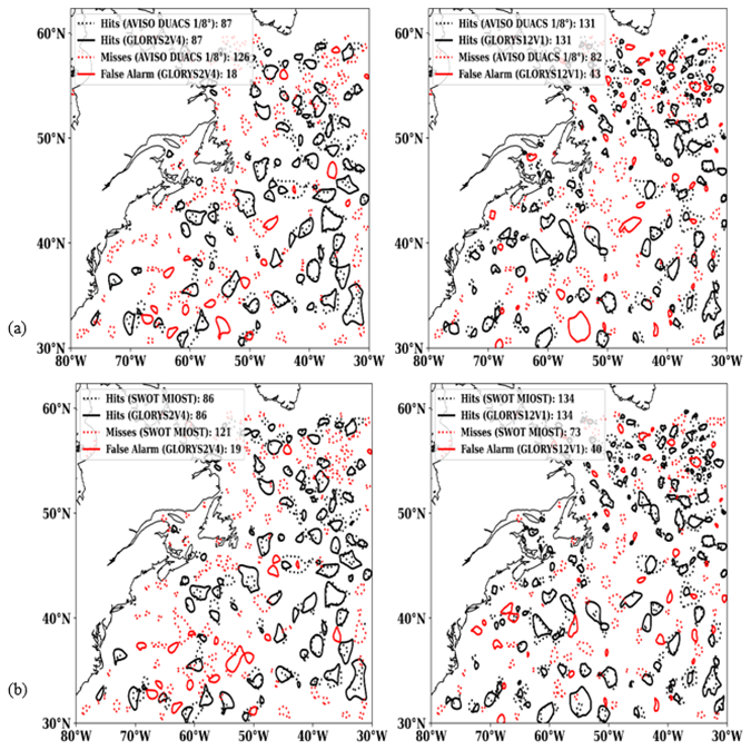
Figure 5 Panel (a) is an example showing Anticyclonic eddy matching statistics for 1 January 2025 for GLORYS2V4 (left), and GLORYS12V1 (right), compared with DUACS. Eddies for which a corresponding match is found (hits) between DUACS and GLORYS2V4/GLORYS12V1 are shown as dotted and solid black contours. Eddies identified in DUACS (satellite data) with no corresponding eddy in GLORYS2V4/GLORYS12V1 are deemed misses (red dotted contours). Eddies identified in GLORYS2V4/GLORYS12V1 but without a corresponding eddy to DUACS are deemed false alarms. Panel (b) is an example showing Anticyclonic eddy matching statistics for 1 January 2025 for GLORYS2V4 (left), and GLORYS12V1 (right), compared with SWOT (satellite data).

The POD is the number of matched eddies over the total number of eddies present in the satellite product.

Similarly, one can consider what fraction of the predicted eddies in the model analyses did not occur using the False Alarm Ratio (FAR), as explained in Smith and Fortin (2022), defined as:

$$\begin{array}{}\text{(3)}& \mathrm{FAR}={\displaystyle \frac{\mathrm{false}\mathrm{alarms}}{(\mathrm{false}\mathrm{alarms}+\mathrm{hits})}}\end{array}$$

Both POD and FAR have values between [0,1] with perfect values of 1 and 0, respectively.

3 Results

In this section, we present the results from the application of the eddy identification, tracking and matching algorithm described above. First, the results of the eddy identification in the four sets of analyses are presented in Sect. 3.1. We then examine the matching statistics (hits, false alarms, misses, POD and FAR) in terms of eddy radius and eddy amplitude in Sect. 3.2. We also evaluate errors in the properties of matched eddies due to the relative contributions to the matching cost function (hits cost, radius, amplitude, and distance between eddy centroids) in Sect. 3.3.

3.1 Results of eddy identification

The properties of identified eddies for the four datasets are quite similar (see Fig. 3) over the entire period (640 d). In Fig. 3, we see similar trends between radius and amplitude. Many small eddies, with a radius lower than 60 km (see Figs. 3 and 4) not far from the threshold of detection, and an amplitude lower than 5 cm, have been identified. We do not clearly see two distinct populations based on an amplitude threshold of 10 cm, compared to the corresponding average lifetime. This is merely a descriptive threshold, intended to show that most of the detected eddies are clustered within a 10 cm amplitude range. For more details, see Appendix C, which provides a more detailed description of the datasets based on specific eddy amplitude thresholds.

In Fig. 4 we see that most have amplitudes below 10 cm, but at the same time there is a moderate positive correlation between amplitude and lifetime, whereby as amplitude increases, so does the average survival time of the eddies. Considering anticyclonic and cyclonic eddies together, the Spearman correlation coefficients are ρ=0.422 for GLORYS12V1, ρ=0.518 for GLORYS2V4, ρ=0.464 for SWOT MIOST Science, and ρ=0.455 for DUACS $\mathrm{1}/\mathrm{8}$°, with p<0.001 in all cases. These results indicate that larger-amplitude eddies tend to persist longer, although the moderate correlation indicates that amplitude alone does not fully explain the variability in eddy lifetime. The number of identified eddies is sensitive to the choice of the minimum eddy lifetime threshold, as noted in Sect. 2.4. Tables 2 and 3 show the total number of anticyclonic and cyclonic eddies detected and tracked with a minimum lifetime of 4 d. The total number of identified and tracked eddies is higher in the satellite products than in GLORYS2V4 and GLORYS12V1, for both anticyclonic and cyclonic eddies. Consistent with its higher spatial resolution, GLORYS12V1 detects more eddies than GLORYS2V4. Tables 2 and 3 also show an almost balanced cyclonic/anticyclonic distribution in the satellite products, but a stronger cyclonic dominance in both reanalyses. This difference is likely related to the different nature of the products. Reanalyses combine assimilated observations with model dynamics and can therefore retain or generate small-scale structures, especially in the eddy-resolving GLORYS12V1 system. In contrast, DUACS and SWOT MIOST are Level-4 gridded satellite products derived from along-track altimetry, and their mapping and interpolation procedures may smooth or merge weak small-scale SSH features. Therefore, the cyclonic excess in the reanalyses should be interpreted with caution. It may reflect model dynamics, data-assimilation effects, and the sensitivity of the closed-contour detection method to weak cyclonic SSH minima, rather than a robust observed polarity asymmetry.

3.2 Eddy verification results

For each comparison, hits, misses, and false alarms are tabulated over the full evaluation period. These counts tabulated, meaning that they are evaluated by adding up all the counts of hits, misses, and false alarms for the entire verification period, for both cyclonic and anticyclonic eddies are used to compute the Probability of Detection (POD) and the False Alarm Ratio (FAR) (following the Eqs. 2 and 3). For the total counts of eddies, the results are reported separately for anticyclonic and cyclonic. The results for DUACS-based comparison are shown in Fig. 6a, Tables 2 and 4, while in Fig. 6b, Tables 3 and 5 for SWOT comparison results.

Table 2 Total number of anticyclonic and cyclonic eddies identified in the region of study over the evaluation period for DUACS, GLORYS2V4, and GLORYS12V1, for a minimum lifetime threshold of 4 d. The percentage of eddies identified in GLORYS2V4 and GLORYS12V1 with respect to DUACS is also provided.

Table 3 Total number of anticyclonic and cyclonic eddies identified in the region of study over the evaluation period for SWOT MIOST, GLORYS2V4, GLORYS12V1, for a minimum lifetime threshold of 4 d. The percentage of eddies identified in GLORYS2V4 and GLORYS12V1 with respect to SWOT MIOST is also provided.

Table 4 Aggregated eddy verification statistics for the Probability of Detection (POD) and False Alarm Ratio (FAR) evaluated over the period, from 1 August 2023 to 1 May 2025, for the comparison with AVISO DUACS $\mathrm{1}/\mathrm{8}$°, with a minimum lifetime threshold of 4 d.

Table 5 Aggregated eddy verification statistics for the Probability of Detection (POD) and False Alarm Ratio (FAR) evaluated over the period 1 August 2023 to 1 May 2025, for the comparison with SWOT MIOST, with a 4 d minimum lifetime threshold.

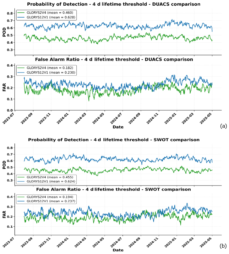
Figure 6 Time series of matching statistics for GLORYS2V4 and GLORYS12V1, compared with DUACS $\mathrm{1}/\mathrm{8}$°, over the period from 1 August 2023 to 1 May 2025, for a 4 d minimum lifetime threshold (a). Bottom panels, the time series with SWOT MIOST Science, over the period from 1 August 2023 to 1 May 2025, for a 4 d minimum lifetime threshold (b).

There is certainly a slight decrease, when comparing the total number of anticyclonic eddies to that of cyclonic eddies, which is particularly evident for GLORYS12V1. Based on the observed data, the two satellite products show nearly balanced polarity counts, with differences not exceeding 1.3 %. In contrast, cyclonic daily detections exceed anticyclonic detections by approximately 7.3 % in GLORYS2V4 and 9.3 % in GLORYS12V1. As shown in the eddy matching example in Fig. 5, there is a significant difference in terms of hits, misses, and false alarms between the two reanalyses. The number of hits increases by about 37 % and the number of misses decreases by about 31 % for both references, while the number of false alarms increases by about 77 % for SWOT and about 83 % for DUACS. This demonstrates how GLORYS12V1 shows greater agreement with both observational datasets, but at the same time generates a significantly higher number of false alarms, which perfectly explains the increase in the FAR, as shown in Fig. 6. Furthermore, the daily POD and FAR fluctuate but remain stationary over time, with no apparent seasonal cycle as shown in Fig. 6a and b. As noted above, the calculation is also applied to the minimum threshold of 7 and 28 d without any observational gaps for each eddy within this time interval, in Appendix A. This sensitivity test shows that short-lived eddies contribute to part of the variability in the verification metrics.

In the aggregated results, GLORYS12V1 achieves a POD exceeding 60 % and a FAR lower than 24 %. For GLORYS2V4, FAR is below 20 %, while POD is close to 46 %. Relative to GLORYS2V4, GLORYS12V1 increases POD by 36.52 % in the DUACS comparison, while FAR increases by 26.37 %. For SWOT, the corresponding relative changes are a 37.14 % increase in POD and a 22.16 % increase in FAR. Mean eddy lifetimes are slightly lower for SWOT than for DUACS for both minimum-lifetime thresholds considered (see Appendix B for more details).

This indicates that, specifically regarding GLORYS2V4, the POD values are very similar in the DUACS and SWOT comparisons. There is a slight decrease when SWOT is used as reference. The decrease is about 0.005 for the 4 d threshold. GLORYS2V4 can match part of the eddies detected by SWOT, but with slightly lower efficiency than for DUACS. The FAR also slightly increases in the SWOT comparison, by about 0.012, showing a small increase in terms of false alarms. Overall, these differences are small, suggesting that the verification results for GLORYS2V4 are relatively insensitive to the choice between the two satellite reference products. However, the overall POD values, which are around 62 %, for both comparisons with GLORYS12V1, show that a significant proportion of observed eddies (around 38 %) remains unmatched. This highlights the presence of limitations in their high-resolution applications, such as difficulties in representing small or short-lived features and maintaining eddy-track continuity. As the minimum lifetime threshold increases, the POD improvement of GLORYS12V1 relative to GLORYS2V4 becomes smaller, whereas the reduction in FAR becomes more pronounced. GLORYS12V1 has a higher FAR than GLORYS2V4 for the 4 and 7 d lifetime thresholds, likely because it detects a larger number of eddies, some of which do not find a corresponding match in the satellite datasets. At the 28 d threshold, this relationship reverses, with GLORYS12V1 showing a lower FAR than GLORYS2V4 (see Appendix A for further details).

To further assess the robustness of these findings, a block bootstrap resampling (95 % confidence intervals) was performed using 4 d blocks, consistent with the imposed minimum lifetime threshold. Results for both SWOT and DUACS (Tables 6 and 7) confirm that GLORYS12V1 systematically outperforms GLORYS2V4 in terms of POD (0.618–0.620 vs. 0.448–0.452), with a statistically significant difference (∼ 0.17) that is insensitive to block length. This gain is consistently associated with a moderate increase in FAR (∼ 0.045–0.049), confirming a robust trade-off between detection sensitivity and reliability. The agreement between the two observational references strengthens confidence in the statistical significance of the results, although it does not fully remove uncertainties related to the definition and detectability of small-scale or short-lived eddy structures.

Table 6 Bootstrap resampling for SWOT MIOST Science comparison, for a minimum lifetime threshold of 4 d, and a block length of 4 d.

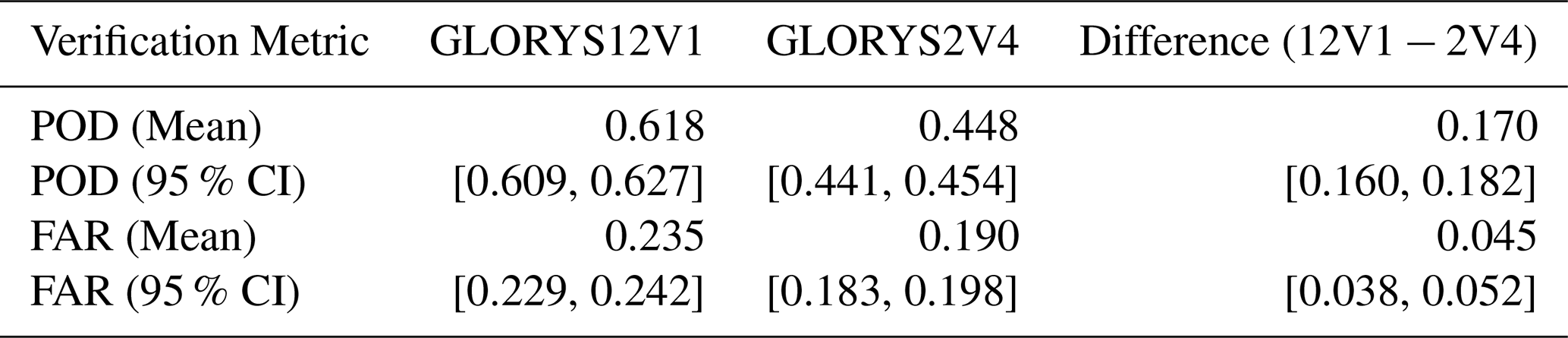
Table 7 Bootstrap resampling for DUACS $\mathrm{1}/\mathrm{8}$° comparison, for a minimum lifetime threshold of 4 d, and a block length of 4 d.

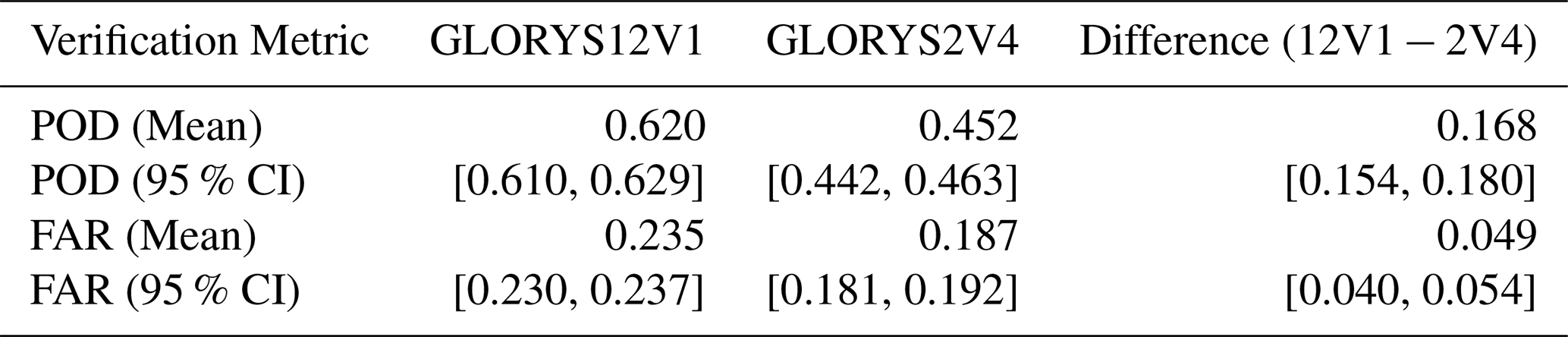
As additional sensitivity tests of the coupled block bootstrap, we also performed the bootstrap resample using 7, 20 and 30 d blocks, and the mean lifetimes of both satellite eddies. The results are reported in Appendix B. The relative ranking of GLORYS12V1 and GLORYS2V4 and the main conclusions of the 4 d analysis remain consistent across the different block lengths, although the estimated confidence intervals vary with the choice of block length. Therefore, the 30 d test is included only as an additional robustness check. Very large block lengths may reduce the variability of the resampling procedure and may partly weaken the main purpose of the block bootstrap, which is to account for temporal dependence in the data when the underlying statistical distribution is unknown.

As the minimum lifetime threshold increases, the POD difference between the two reanalyses decreases. The FAR difference narrows at 7 d and reverses sign at 28 d, when GLORYS12V1 has a lower FAR than GLORYS2V4 for both observational references. Figures 7 and 9 show the dependence of the eddy matching statistics (hits, misses and false alarms) on the physical properties of the eddies, namely the effective radius and amplitude, respectively. These statistics are calculated to show how eddies are distributed across different ranges of radius and amplitude, and thus to identify the ranges with the highest clustering. For hits and misses, the radius and amplitude were taken from the satellite (the reference) product, because these eddies refer to observed features that are either detected or not detected by the reanalysis. For false alarms, the radius and amplitude are taken from the corresponding reanalysis product. Each bin of the histogram has a width of 10 km and 2 cm, respectively for eddy radius and eddy amplitude. The highest counts of misses and false alarms are associated with small eddies, specifically for those with radii below 50 km and amplitudes below 5 cm.

Figures 8 and 10 show the dependence of the verification metrics in terms of the same physical eddy features.

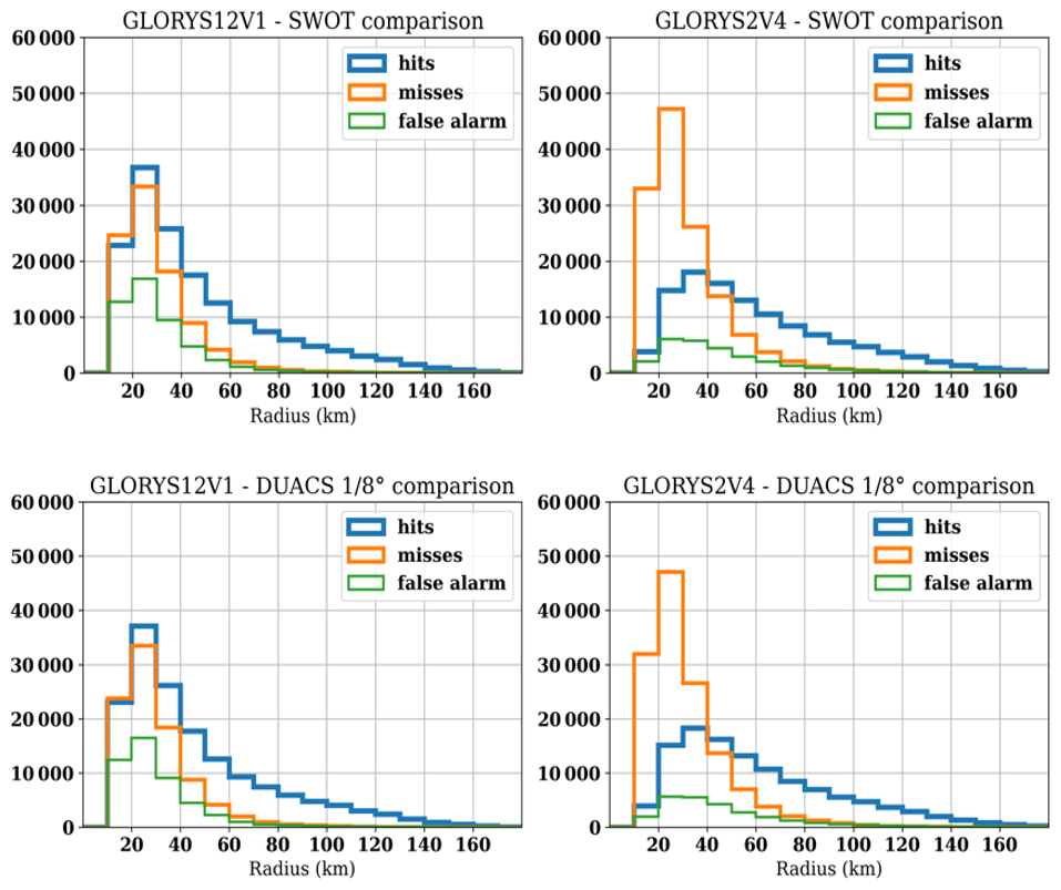
Figure 7 Top panels: eddy matching histograms for the total number of hits (blue), misses (orange), false alarms (green) for GLORYS12V1 (left) and GLORYS2V4 (right), compiled as a function of effective radius (km) over the evaluation period, for SWOT comparison, with a lifetime threshold of 4 d. Bottom panels: eddy matching histograms compiled as a function of effective radius (km) over the same evaluation period, for comparison with DUACS, with a lifetime threshold of 4 d. The radius of hits and misses refers to the satellite (reference) eddies, whereas the radius of false alarms refers to unmatched eddies detected in the reanalysis.

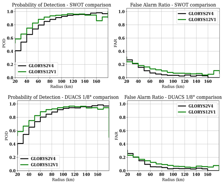
Figure 8 Top panels: histograms of the probability of detection (POD; left) and the false alarm ratio (FAR; right), over the evaluation period, evaluated as a function of radius (km) for comparison with SWOT, with a lifetime threshold of 4 d. Bottom panels: histograms of the POD and FAR as a function of radius (km), for the comparison with DUACS, with a lifetime threshold of 4 d. The radius of hits and misses refers to the satellite (reference) eddies, whereas the radius of false alarms refers to unmatched eddies detected in the reanalysis.

Figure 9 Top panels: eddy matching histograms for the total number of hits (blue), misses (orange), false alarms (green) for GLORYS12V1 (left) and GLORYS2V4 (right), compiled as a function of amplitude (cm) over the evaluation period, for SWOT comparison. Bottom panels: eddy matching histograms compiled as a function of amplitude (cm) over the evaluation period, for comparison with DUACS $\mathrm{1}/\mathrm{8}$°. The amplitude of hits and misses refers to the satellite (reference) eddies, while the amplitude of false alarms refers to those of unmatched eddies, detected in the reanalysis.

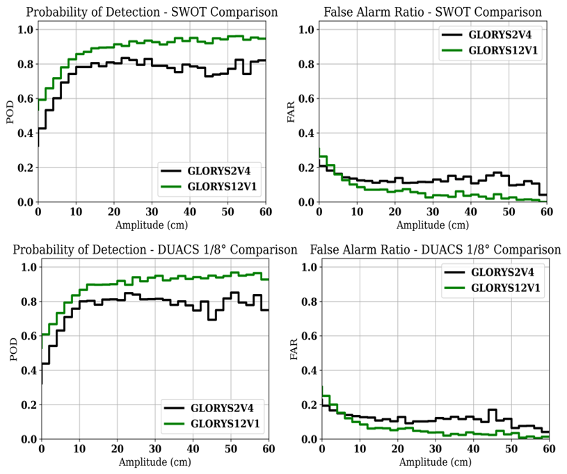
Figure 10 Top panels: histograms of the probability of detection (POD; left) and the false alarm ratio (FAR; right), over the evaluation period, evaluated as a function of amplitude (cm) for comparison with SWOT. Bottom panels: histograms of the POD and FAR as a function of amplitude (cm), over the evaluation period, for the comparison with DUACS. The amplitude of hits and misses refers to the satellite (reference) eddies, while the amplitude of false alarms refers to those of unmatched eddies detected in the reanalysis.

For the DUACS comparison, Figs. 8 and 10 show that FAR is generally higher in the smallest effective-radius and amplitude bins, exceeding 30 % in some of these classes and highlighting the greater difficulty in verifying the smallest features in this gridded product. The FAR remains close or higher than 20 % until 50 km in terms of effective radius. At the same time, the POD of GLORYS12V1 is close to 60 % even for small radius and amplitude values, showing a relevant fraction of small observed eddies is still detected by the reanalyses. The largest proportion of misses is consistently associated with small eddies, specifically those with radii below 50 km and amplitudes under 4 cm. The comparison with SWOT shows a similar dependence on eddy size. The largest differences in the verification metrics are again found for small-radius and small-amplitude eddies. The POD of GLORYS12V1 remains close to 60 %, while the GLORYS2V4 FAR is generally higher in the smallest bins. This indicates that the main difficulty is not only the detection of small observed eddies, but also the presence of unmatched (especially for the small eddies) produced by the reanalyses. However, for both satellite comparisons, the verification skills generally improve as eddy radius and amplitude increase. This suggests a better matching capability for larger and stronger mesoscale eddies, which are less affected by small-scale noise or detection uncertainty. The differences between the DUACS and SWOT comparison are most evident for small eddies, while they become smaller for larger eddies. For this reason, Appendix C includes additional analyses of the verification metrics using different amplitude-based subsets, including eddies with amplitudes greater than 5, 10, 15, and 20 cm, as well as eddies with amplitudes below 10 cm. Appendix C also presents the eddy matching histograms using a semi-logarithmic scale for the y-axis, which represents the number of eddies. These additional analyses allow us to assess more clearly how the verification results change when low-amplitude eddies are progressively excluded, when the analysis focuses on stronger mesoscale structures, and when the contribution of the most numerous small-amplitude eddies is examined in greater detail.

Small-eddy detections are more sensitive to mapping, filtering, observational noise, model resolution, and the parameters of the detection and tracking algorithms. Consequently, the smallest bins may contain both dynamically relevant eddies and uncertain or spurious detections. Potential contributors include incomplete along-track sampling in mapped altimetry and assumptions in the SAM2 background-error covariance (Lellouche et al., 2018).

For eddies larger than these limits, both comparisons show strong agreement. In DUACS comparison, for radii > 100 km, the POD reaches ∼ 90 % and FAR falls to around 10 %–15 %. In the SWOT-based comparison, the performance is quite similar: FAR drops below 10 %, while POD rises above 80 %–95 % for amplitudes greater than 10 cm.

An additional perspective on the differences between GLORYS12V1 and GLORYS2V4 can be obtained by examining the integrated matching statistics as a function of eddy radius and amplitude (Figs. 11 and 12). We focus on two descriptive diagnostics: (i) the radius below which 90 % of the false alarms occur and (ii) the percentage of matched eddies with amplitudes greater than 10 cm. The first identifies the size range in which unmatched reanalysis detections are concentrated, whereas the second describes the contribution of high-amplitude eddies to successful matches. These values are used for descriptive comparison and should not be interpreted as physical thresholds defining separate eddy populations or as criteria for filtering detections.

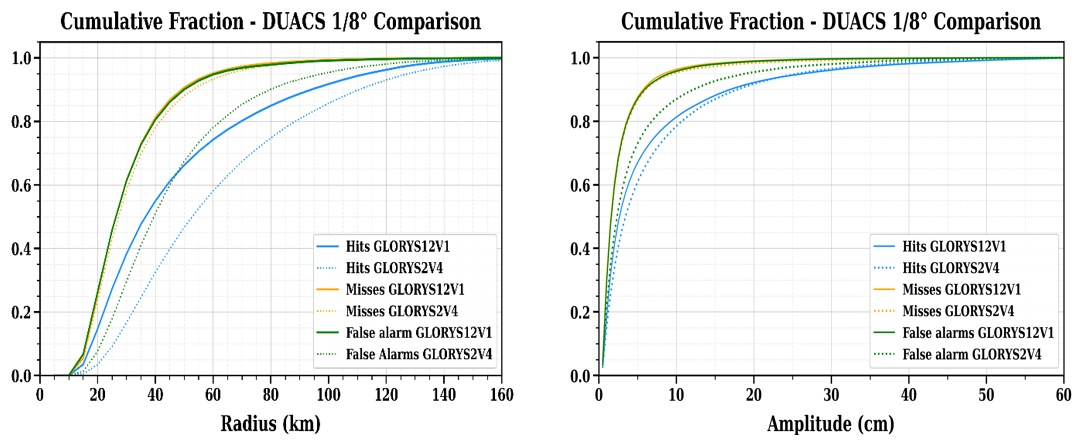
Figure 11 Cumulative distribution of hits (blue), misses (orange) and false alarms (green) for GLORYS2V4 (dotted) and for GLORYS12V1 (solid) as a function of radius (left) and amplitude (right), for the comparison with DUACS, with a lifetime threshold of 4 d. The radius and the amplitude of hits and misses refer to the satellite (reference) eddies, while the radius and the amplitude of false alarms refer to the unmatched eddies detected in the reanalysis.

Figure 12 Cumulative distribution of hits (blue), misses (orange) and false alarms (green) for GLORYS2V4 (dotted) and for GLORYS12V1 (solid) as a function of radius (left) and amplitude (right), for the comparison with SWOT, with a lifetime threshold of 4 d. The radius and the amplitude of hits and misses refer to the satellite (reference) eddies, while the radius and the amplitude of false alarms refer to the unmatched eddies detected in the reanalysis.

For DUACS comparison (Fig. 11), we can see that:

• 90 % of false alarms are concentrated below the 49.9 km radius for GLORYS12V1 and 79.7 km for GLORYS2V4, corresponding to a difference of 29.8 km between the two cumulative distributions. Regarding Amplitude, 95.63 % of GLORYS12V1 hits and 86.93 % of GLORYS2V4 hits occur below 10 cm.

We estimate that 4.37 % of GLORYS12V1 hits are above 10 cm, compared with 13.07 % for GLORYS2V4, a difference of 8.70 percentage points.

For the SWOT comparison, using the results of Fig. 12, we can estimate:

• 90 % of false alarms fall below 52.70 km radius for GLORYS12V1 and 80.30 km for GLORYS2V4, corresponding to a difference of 27.60 km. In terms of amplitude, 87.1 % of GLORYS2V4 hits and 95.55 % of GLORYS12V1 hits lie below 10 cm.

For SWOT, the corresponding proportions above 10 cm are 12.9 % for GLORYS2V4 and 4.45 % for GLORYS12V1, a difference of −8.45 percentage points (GLORYS12V1 – GLORYS2V4).

Thus, the proportion of matched eddies exceeding 10 cm is smaller for GLORYS12V1 in both comparisons. Similar statements can be made for eddy radius.

Overall, these cumulative diagnostics show that most matching errors are associated with small eddies, those with radii below 50 km and amplitude below 4–5 cm. We see differences between DUACS and SWOT comparisons. They should be interpreted only as differences in reanalysis–satellite consistency over the common evaluation period, and not as a ranking of the quality of the two satellite products. However it also confirms a key weakness of GLORYS12V1: although it detects more eddies overall, it also produces more unmatched eddies (small eddies), which increases FAR. These cumulative plots show that both reanalysis systems still struggle to match very small eddies (radius < 50 km and amplitude < 4–5 cm), and that some of these features may represent uncertain or spurious detections rather than robust mesoscale eddies. This suggests that future verification studies should apply filters to remove or down-weight small eddies, so that evaluation focuses on dynamically meaningful ocean structures.

3.3 Evaluation of errors in matched eddy properties

Determining whether an observed eddy has a corresponding match in a reanalysis dataset is important, but it does not fully capture how accurately that eddy is represented. As illustrated in Fig. 5, and explained in Sect. 2.4, some matched eddies exhibit significant differences in terms of radius, amplitude, position, compared to the satellite data, despite correctly identifying the same features (see Eq. 1). These discrepancies are expected to vary between the two reanalysis systems given their differing spatial resolutions, and thus their capacity to resolve mesoscale variability. We therefore assess whether the properties of matched eddies differ between the two reanalysis systems. To quantify these differences, we analyze the errors in radius, amplitude, and centre displacements for each “matched” eddy (hit). For each of these properties, we compute binned, normalized histograms that illustrate the distribution of radius error (difference between satellite and reanalysis effective radius), amplitude error (difference in SSH extremum relative to the outer contour between satellite and reanalysis matched eddy), separation distance between satellite and reanalysis matched eddy centroid.

Unlike the tracking cost function (Eq. 1), these quantities are presented without the normalization factors (i.e., not scaled by A₁, R₁, or the 125 km distance), to retain their physical units (km or cm). While this approach no longer allows a direct assessment of their relative contribution to the overall cost function, it provides a clearer, physically interpretable picture of where and how the reanalyses diverge from satellite data (facilitates a physical interpretation of the histograms). The resulting normalized histograms (normalized by the total number of hits) are shown in Fig. 13a and b. The distributions of the cost function and associated errors for matched eddies reveal clear differences between GLORYS2V4 and GLORYS12V1, for all terms of the cost function (Eq. 1). Indeed, from Table 8, the mean cost function values, for DUACS comparison, are 1.76 for GLORYS2V4 and 1.31 for GLORYS12V1, indicating a clear reduction in the cost function for each matched eddy for the eddy-resolving (GLORYS12V1) system. Likewise, the mean errors in effective radius (24.62 km vs. 16.81 km), the mean amplitude errors (5.43 cm vs. 3.55 cm) and centroid distance (57.49 km vs. 49.85 km) are quite different with general differences between the two reanalysis systems.

Table 8 Mean error contributions to the cost function for all hits evaluated over the period from 1 August 2023 to 1 May 2025 for the DUACS comparison. Mean values are shown for the total cost and for the radius (km), amplitude (cm), and centroid-distance (km) errors. The percentage change from GLORYS2V4 to GLORYS12V1 is reported in the final row.

Table 9 Mean error contributions to the cost function for all hits evaluated over the period from 1 August 2023 to 1 May 2025 for the SWOT comparison. Mean values are shown for the total cost and for the radius (km), amplitude (cm), and centroid-distance (km) errors. The percentage change from GLORYS2V4 to GLORYS12V1 is reported in the final row.

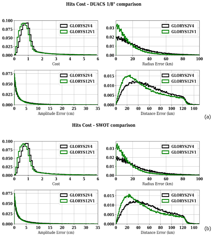
Figure 13 In (a), normalized histograms of values for matched eddies between DUACS and GLORYS2V4 (black line) or GLORYS12V1 (green line). Panel (b) shows the corresponding comparison between SWOT and GLORYS2V4 or GLORYS12V1. The distribution of values for the total cost is shown in the top panel on the left. Also shown are the normalized distributions of differences in terms of radius in the top on the right, amplitude in the bottom on the left, and distance between eddy positions, in the bottom on the right.

For SWOT comparison (see Table 9), the differences between the two reanalyses become somewhat more pronounced than in the DUACS comparison, for all terms of cost function (most notably in the error regarding the effective radius, but except for the distance between the centroid of eddies). The mean cost function is 1.79 for GLORYS2V4 and 1.33 for GLORYS12V1, corresponding to a −25.70 % difference, crossing from GLORYS2V4 to GLORYS12V1. The amplitude error is 5.53 cm vs. 3.59 cm (−35.08 % in difference, from GLORYS2V4 to GLORYS12V1). The effective radius error is 24.92 km versus 16.79 km (−32.62 % in difference) and the centroid distance error is 57.86 km vs. 50.29 km (−13.08 % in difference). These results indicate that, for all terms of the cost function, GLORYS12V1 achieves nearly identical results in both comparisons (Tables 8 and 9). Meanwhile, GLORYS2V4 shows slightly higher average values for all terms of the cost function when compared to SWOT. These results show that GLORYS12V1 has lower mean errors than GLORYS2V4 for all terms of the cost function in both satellite comparisons. The improvement is particularly evident for the effective radius and amplitude errors, while the reduction in centroid-distance error is smaller but still present. This confirms that the eddy-resolving reanalysis provides a better representation of the physical properties of matched eddies. The advantage of GLORYS12V1 becomes slightly more apparent when the comparison is performed against SWOT. However, the results for the SWOT and DUACS comparisons are very similar. This shows that the relative improvement of GLORYS12V1 over GLORYS2V4 is robust to the choice of satellite reference dataset.

4 Summary and discussion

We have applied a feature-based verification methodology for evaluating ocean reanalysis products, following the verification approach developed and adopted by Smith and Fortin (2022), and we have used the eddy detection and tracking procedures described in Mason et al. (2014) and Pegliasco et al. (2021). This methodology is based on prior work in eddy tracking and leverages open-source tools (py-eddy-tracker) to provide a robust, reproducible framework for assessing the skill of reanalysis datasets in representing observed mesoscale features. As a demonstration, we evaluated eddy properties in two global reanalysis systems of different spatial resolutions, GLORYS2V4 and GLORYS12V1, from 1 August 2023 to 1 May 2025 for both comparisons.

The analysis shows a significant increase in POD for GLORYS12V1 compared with GLORYS2V4, although this improvement is accompanied by a higher FAR under the 4 d reference configuration. The verification results show clear differences between the two reanalyses when evaluated against the satellite reference products. When compared with DUACS, GLORYS12V1 achieves a POD of 0.628, compared with 0.460 for GLORYS2V4, corresponding to a relative increase of approximately 37 %. However, FAR increases from 0.182 to 0.230, corresponding to a relative increase of approximately 26 %. The comparison with SWOT MIOST Science shows similar results: POD is 0.624 for GLORYS12V1 and 0.455 for GLORYS2V4, corresponding to an increase of approximately 37 %, while FAR increases from 0.194 to 0.237, or by approximately 22 %. The block-bootstrap analysis performed using a 4 d minimum lifetime threshold and 4 d blocks confirms this difference. The mean FAR difference between GLORYS12V1 and GLORYS2V4 is 0.049 for DUACS (95 % CI: [0.040, 0.054]) and 0.045 for SWOT MIOST Science (95 % CI: [0.038, 0.052]). Further block-bootstrap sensitivity tests, reported in Appendix B, were performed using 7, 20, and 30 d blocks, as well as block lengths based on the mean lifetimes of the satellite-observed eddies. These tests provide consistent results. In all these tests, the 95 % confidence interval of the FAR difference remains above zero. Therefore, the higher FAR of GLORYS12V1 is robust to the choice of block length, although the difference between the two reanalyses becomes smaller when the 7 d minimum lifetime threshold is applied. Small and short-lived eddies play an important role in the verification results. The sensitivity analyses using minimum-lifetime thresholds of 7 and 28 d are reported in Appendix A. The differences between GLORYS12V1 and GLORYS2V4 decrease as the minimum-lifetime threshold increases, particularly for FAR. The FAR gap narrows at the 7 d threshold and reverses at the 28 d threshold: GLORYS12V1 retains higher POD and has lower FAR than GLORYS2V4 for both observational references when only long-lived eddies are retained. This behaviour is associated with the exclusion of many short-lived and less stable eddies, which are among the most difficult features to match across datasets. For matched eddies, GLORYS12V1 also provides a more accurate representation of eddy properties. For both satellite comparisons, its mean matching cost is approximately 26 % lower than that of GLORYS2V4, while the mean errors in effective radius, amplitude, and centroid distance are reduced by approximately 32 %, 35 %, and 13 %, respectively.

The concentration of misses and false alarms among small eddies indicates greater uncertainty in their detection and matching. Some of these features may correspond to dynamically relevant eddies, whereas others may be affected by noise, mapping uncertainties, filtering, or unresolved variability. GLORYS12V1 detects a larger number of small features, some of which remain unmatched and contribute to its higher FAR. This highlights the need for a simple and objective approach to limit the influence of very small and short-lived eddies in both satellite products and reanalyses, in order to obtain more reliable verification metrics. The sensitivity tests in Appendix D show that the absolute POD and FAR values depend on the matching-distance threshold and the Bessel-filter cutoff wavelength. Nevertheless, GLORYS12V1 maintains a higher POD than GLORYS2V4 under all the tested configurations.

Both satellite reference products are distributed on a nominal $\mathrm{1}/\mathrm{8}$° grid, while SWOT MIOST Science additionally incorporates wide-swath SWOT observations through the MIOST mapping methodology. However, the Copernicus Marine Service Synthesis Quality Overview Document for Sea Level Products (CMEMS-SL-SQO-008-033-068) (Copernicus Marine Service, 2026) notes that the effective resolution of gridded sea-level products remains constrained by altimeter sampling and mapping procedures. Therefore, caution is required when interpreting results close to the effective resolution limit, because very small and short-lived eddies may still be influenced by noise and mapping artefacts. The remapping of all datasets onto the same regular $\mathrm{1}/\mathrm{8}$° grid allows a consistent comparison but does not make their native or effective resolutions equivalent. Despite these limitations, the results support the added value of the eddy-resolving GLORYS12V1 reanalysis compared with the eddy-permitting GLORYS2V4. The amplitude-based analyses show that GLORYS12V1 generally maintains a higher POD than GLORYS2V4. However, progressively excluding low-amplitude eddies does not produce a monotonic improvement in POD and FAR, as shown in Appendix C. False alarms are mainly concentrated among small eddies. In the DUACS comparison, 90 % of the false alarms occur below a radius of approximately 50 km for GLORYS12V1 and 80 km for GLORYS2V4. The corresponding thresholds in the SWOT comparison are approximately 53 and 80 km. These results indicate that the false alarms associated with GLORYS12V1 are concentrated at smaller radii; they do not imply a lower total number or ratio of false alarms. In the DUACS comparison, approximately 4.3 % of the GLORYS12V1 hits have amplitudes above 10 cm, compared with 13.1 % for GLORYS2V4. In the SWOT comparison, the corresponding proportions are approximately 4.5 % and 12.9 %, respectively. These values describe the amplitude distribution of the matched eddies and should not be interpreted as direct measures of the overall performance of the two reanalyses. The common evaluation period covers less than two years and may therefore not fully sample the interannual variability of the North Atlantic eddy field. This limitation is particularly relevant for large and energetic eddies, which are less frequent and more sensitive to the specific dynamical conditions of the analysed period. Moreover, the results should not be interpreted as a ranking of the quality of the two satellite products. DUACS and SWOT MIOST Science provide complementary observational references with different mapping characteristics and levels of small-scale variability. SWOT MIOST Science provides additional information from wide-swath observations, but it remains a Level-4 mapped product. Furthermore, neither satellite product can be considered a fully independent reference because they share nadir-altimetry information with each other and with observations assimilated into the reanalyses.

Future work should develop objective and scale-aware strategies to filter or down-weight uncertain small features without automatically excluding dynamically relevant eddies. The present matching and verification framework could also be extended to include the “coincidence status” classification described by Ma et al. (2020), distinguishing matched, split, merged, missed, and artefactual eddies. This would provide a more detailed assessment and improve the diagnostic capability of the verification framework. Finally, extending the analysis to longer periods, using satellite products with sufficient temporal coverage, and applying the methodology to other ocean regions would make it possible to better account for interannual variability and different dynamical regimes.

Appendix A

In this appendix we aim to assess how the verification metrics, used to evaluate the ability of global ocean reanalyses to detect eddies observed in satellite datasets over a highly eddy-populated region, change under these different methodological choices.

A1 Eddy detection-tracking and matching results for minimum-lifetime thresholds of 7 and 28 d

To assess the sensitivity of the verification results to the lifetime criterion, the detection, tracking, and matching analyses were repeated using minimum-lifetime thresholds of 7 and 28 d. Tables A1, A2, A5, and A6 report the numbers of anticyclonic and cyclonic eddies retained in each catalogue, whereas Tables A3, A4, A7, and A8 report POD, FAR, and the differences between GLORYS12V1 and GLORYS2V4. Increasing the minimum lifetime substantially reduces the number of retained eddies, especially at 28 d. In Fig. A1, panel (a) shows the time series of the verification metrics over the full study period for both comparisons, while panel (b) shows the power spectra associated with each time series. The power spectra are used to assess how the variability of the verification metrics changes as the minimum eddy lifetime threshold increases.

At the 7 d threshold, POD decreases for both reanalyses. FAR increases for GLORYS2V4, whereas for GLORYS12V1 it decreases slightly against DUACS and remains essentially unchanged against SWOT. At the 28 d threshold, POD decreases and FAR increases relative to the 4 d configuration. Nevertheless, GLORYS12V1 retains a higher POD and a lower FAR than GLORYS2V4 for both references. This indicates that, among long-lived eddies, GLORYS12V1 matches a larger fraction of observed eddies and has a lower proportion of unmatched reanalysis detections. The GLORYS12V1 FAR becomes lower than that of GLORYS2V4 when only long-lived eddies are considered. However, the application of a longer lifetime threshold also leads to a substantial reduction in the total number of detected and tracked eddies compared to the lower lifetime cases, as shown in Tables A1, A2, A5, and A6. Compared with the 4 d threshold, the reduction in the number of retained eddies at 28 d is strongest for GLORYS12V1, whereas it is slightly weaker for GLORYS2V4 than for the satellite datasets. Nevertheless, the 28 d threshold leads to an overall decrease in POD and an overall increase in FAR for both comparisons and for both reanalysis products relative to the results discussed in Sect. 3.2 and reported in Tables 4 and 5. This behaviour indicates that, although the 28 d threshold isolates more stable eddy structures, it also exposes a significant discrepancy between the reanalyses and the observational datasets. In particular, some of the eddies matched in the reanalyses at lower lifetime thresholds appear to be less temporally stable than those observed in the satellite products. As a result, the number of hits clearly tends to decrease as the minimum lifetime threshold increases.

This sensitivity test therefore suggests that temporally more stable eddies tend to reduce the resolution-related gap between the two reanalysis products. Nevertheless, this does not lead to an increase in POD or to a systematic decrease in FAR. This confirms that both ocean reanalyses still show limitations in capturing observed eddies and in avoiding the generation of unmatched eddy-like structures. More generally, these results show that one of the main challenges is to identify a method capable of removing spurious and unstable structures, for which it is not always clear whether they can be considered robust mesoscale eddies.

In panel (b), the power spectra show that, at short temporal scales, the variability of the verification-metric time series is similar across the different configurations. The spectral differences are mainly concentrated at the longest resolved periods. For FAR, GLORYS12V1 has the larger peak with the 7 d threshold, whereas GLORYS2V4 has the larger peak with the 28 d threshold. Because the analysed record is only 640 d long, peaks at periods of 320–640 d should be interpreted as low-frequency variability rather than as evidence of robust periodic or seasonal signals. It should also be noted that the axes do not have the same numerical range across all panels. In general, the numerical range of the FAR power spectra is larger than that of POD, indicating that the strongest spectral peaks are generally associated with FAR.

Table A1 Total number of anticyclonic and cyclonic eddies identified in the region of study over the evaluation period for DUACS, GLORYS2V4, and GLORYS12V1, for eddies with a minimum lifetime threshold of 7 d. The percentage of eddies identified in GLORYS2V4 and GLORYS12V1 with respect to DUACS is also provided.

Table A2 Total number of anticyclonic and cyclonic eddies identified in the region of study over the evaluation period for SWOT, GLORYS2V4, and GLORYS12V1, for eddies with a minimum lifetime threshold of 7 d. The percentage of eddies identified in GLORYS2V4 and GLORYS12V1 with respect to SWOT is also provided.

Table A3 Aggregated eddy verification statistics for the Probability of Detection (POD) and False Alarm Ratio (FAR) evaluated over the period, from 1 August 2023 to 1 May 2025, for the comparison with DUACS, with a minimum lifetime threshold of 7 d.

Table A4 Aggregated eddy verification statistics for the Probability of Detection (POD) and False Alarm Ratio (FAR) evaluated over the period, from 1 August 2023 to 1 May 2025, for the comparison with SWOT, with a minimum lifetime threshold of 7 d.

Table A5 Total number of anticyclonic and cyclonic eddies identified in the region of study over the evaluation period for DUACS, GLORYS2V4, and GLORYS12V1. The percentage of eddies identified in GLORYS2V4 and GLORYS12V1 with respect to DUACS is also provided, with a lifetime threshold of 28 d.

Table A6 Total number of anticyclonic and cyclonic eddies identified in the region of study over the evaluation period for SWOT, GLORYS2V4, and GLORYS12V1. The percentage of eddies identified in GLORYS2V4 and GLORYS12V1 with respect to SWOT is also provided, with a lifetime threshold of 28 d.

Table A7 Aggregated eddy verification statistics for the Probability of Detection (POD) and False Alarm Ratio (FAR) evaluated over the period, from 1 August 2023 to 1 May 2025, for the comparison with DUACS, with a minimum lifetime threshold of 28 d.

Table A8 Aggregated eddy verification statistics for the Probability of Detection (POD) and False Alarm Ratio (FAR) evaluated over the period, from 1 August 2023 to 1 May 2025, for the comparison with SWOT, with a minimum lifetime threshold of 28 d.

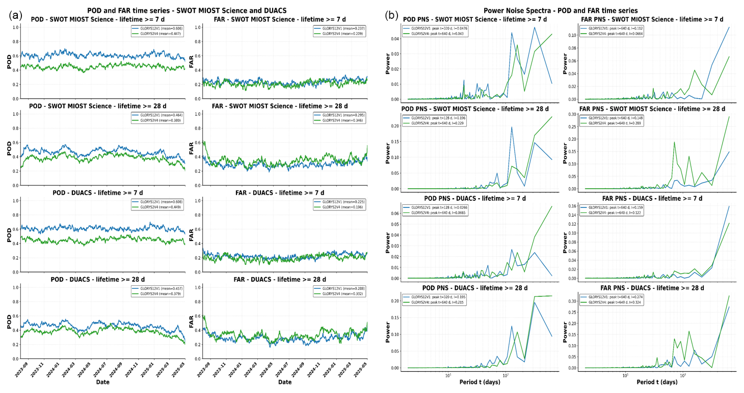
Figure A1 Time series of matching statistics for GLORYS2V4 and GLORYS12V1, compared with SWOT and DUACS (a), over the period from 1 August 2023 to 1 May 2025, with a minimum lifetime of 7 and 28 d. In (b), the power spectra of each time series, for both products and comparisons.

Appendix B

B1 Sensitivity of bootstrap resampling results for verification metrics to the block length

To assess the sensitivity of the confidence intervals to temporal dependence, the coupled block-bootstrap analysis was repeated using block lengths of 7, 20, and 30 d, as well as block lengths derived from the mean lifetimes of the satellite-observed eddies. Results are reported for the 4 and 7 d minimum-lifetime thresholds. Across the tested block lengths, GLORYS12V1 maintains higher POD than GLORYS2V4 for both observational references. The FAR difference also remains positive, although it becomes smaller for the 7 d minimum-lifetime threshold.

For the sake of completeness, we also calculated the average lifetimes of the observed eddies for each satellite dataset using two different minimum lifetimes (4 and 7 d). The idea is to use these average lifetimes as the block lengths for the coupled bootstrap resampling. The mean eddy lifetime is calculated from the number of daily observations associated with each individual trajectory, using the “nb_obs_by_track” property provided by py-eddy-tracker. Tracks with zero observations are excluded.

For DUACS, we calculate the average lifetime of eddies:

• Anticyclonic eddies with a minimum lifetime threshold of 4 d: 18.03 d.

• Cyclonic eddies with a minimum lifetime threshold of 4 d: 18.23 d.

• Anticyclonic eddies with a minimum lifetime threshold of 7 d: 22.69 d.

• Cyclonic eddies with a minimum lifetime threshold of 7 d: 23.05 d.

Therefore, considering both anticyclonic and cyclonic eddies, we calculate an average eddy lifetime of: 18.13 d (minimum lifetime of 4 d) and 22.87 d (minimum lifetime of 7 d). Therefore, for the block bootstrap resample, we rounded up to the next whole day, setting a value of 19 d for a minimum lifetime of 4 d, and a value of 23 d for a minimum lifetime of 7 d.

For SWOT, we calculate the average lifetime of eddies:

• Anticyclonic eddies with a minimum lifetime threshold of 4 d: 17.51 d.

• Cyclonic eddies with a minimum lifetime threshold of 4 d: 17.58 d.

• Anticyclonic eddies with a minimum lifetime threshold of 7 d: 22.69 d.

• Cyclonic eddies with a minimum lifetime threshold of 7 d: 22.38 d.

Therefore, considering both anticyclonic and cyclonic eddies, we calculate an average eddy lifetime of: 17.54 d (minimum lifetime of 4 d) and 22.54 d (minimum lifetime of 7 d). Therefore, for the block bootstrap resample, we rounded up to the next whole day, setting a value of 18 d for a minimum lifetime of 4 d, and a value of 23 d for a minimum lifetime of 7 d.

Table B1 Bootstrap resampling for SWOT, for a minimum lifetime threshold of 7 d and a block length of 7 d.

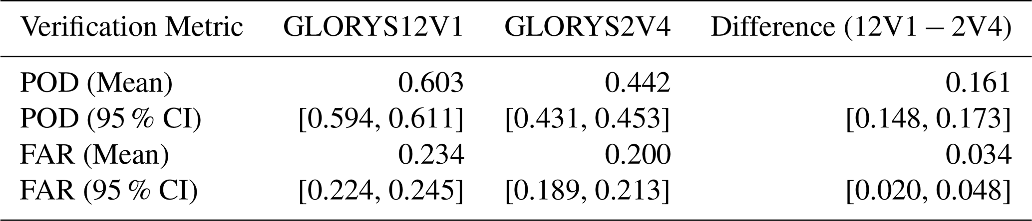
Table B2 Bootstrap resampling for DUACS comparison, for a minimum lifetime threshold of 7 d and a block length of 7 d.

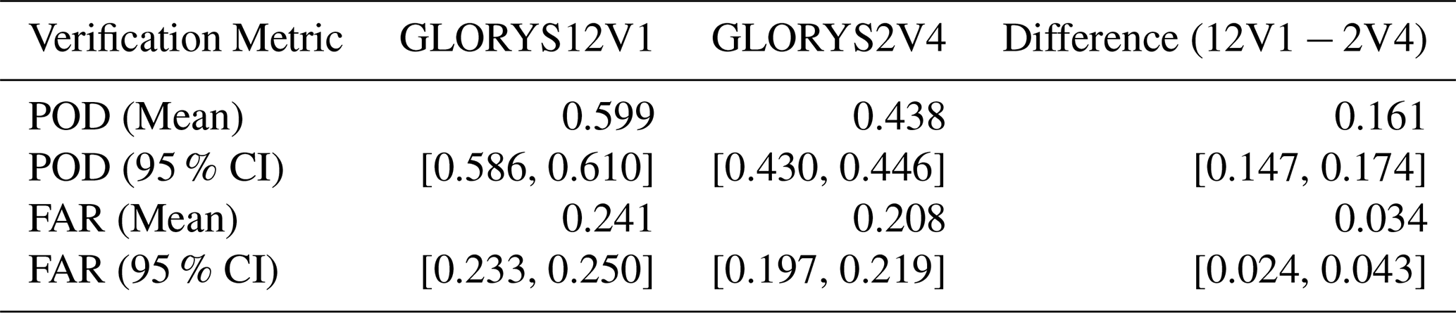
Table B3 Block-bootstrap estimates of POD and FAR using 20 d blocks for the comparison with DUACS. Values are reported for GLORYS12V1, GLORYS2V4, and their difference, together with 95 % confidence intervals. In the first row, there is the calculation for the 4 d minimum lifetime threshold. In the second row, there is the calculation for 7 d minimum lifetime threshold.

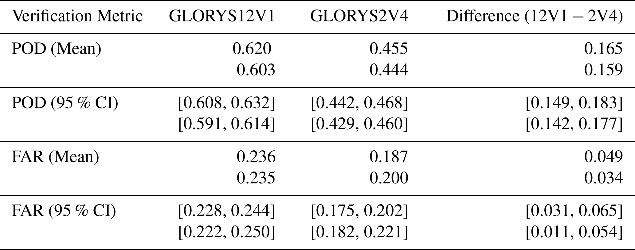
Table B4 Block-bootstrap estimates of POD and FAR using 20 d blocks for the comparison with SWOT MIOST. Values are reported for GLORYS12V1, GLORYS2V4, and their difference, together with 95 % confidence intervals. In the first row, there is the calculation for the 4 d minimum lifetime threshold. In the second row, there is the calculation for 7 d minimum lifetime threshold.

Table B5 Block-bootstrap estimates of POD and FAR using 30 d blocks for the comparison with DUACS. Values are reported for GLORYS12V1, GLORYS2V4, and their difference, together with 95 % confidence intervals. In the first row, there is the calculation for the 4 d minimum lifetime threshold. In the second row, there is the calculation for 7 d minimum lifetime threshold.

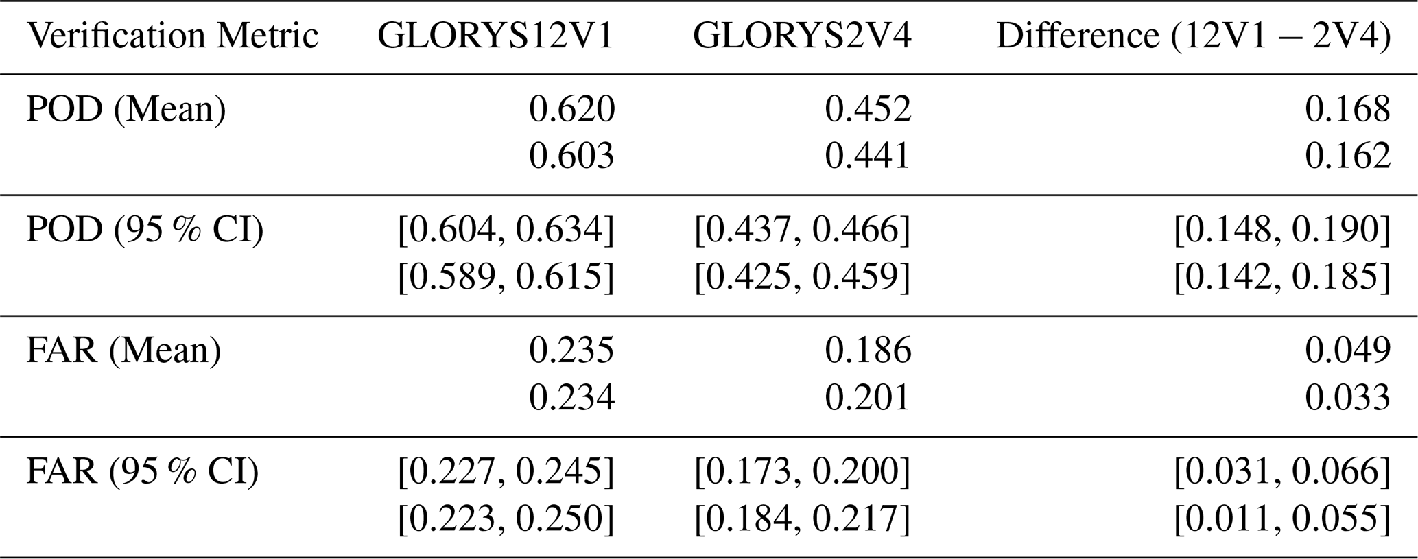
Table B6 Block-bootstrap estimates of POD and FAR using 30 d blocks for the comparison with SWOT. Values are reported for GLORYS12V1, GLORYS2V4, and their difference, together with 95 % confidence intervals. In the first row, there is the calculation for the 4 d minimum lifetime threshold. In the second row, there is the calculation for 7 d minimum lifetime threshold.

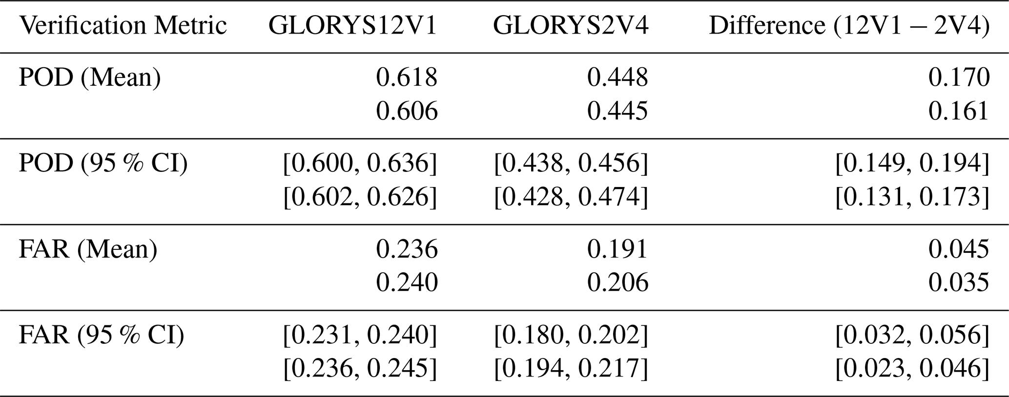
Table B7 Block-bootstrap estimates of POD and FAR for the comparison with DUACS, using a 19 d block length for the 4 d minimum-lifetime threshold and a 23 d block length for the 7 d minimum-lifetime threshold. Values are reported for GLORYS12V1, GLORYS2V4, and their difference, together with 95 % confidence intervals.

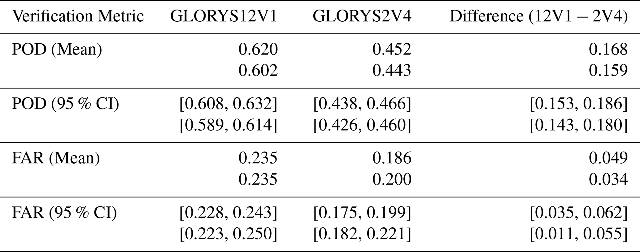
Table B8 Block-bootstrap estimates of POD and FAR for the comparison with SWOT, using an 18 d block length for the 4 d minimum-lifetime threshold and a 23 d block length for the 7 d minimum-lifetime threshold. Values are reported for GLORYS12V1, GLORYS2V4, and their difference, together with 95 % confidence intervals.

Appendix C

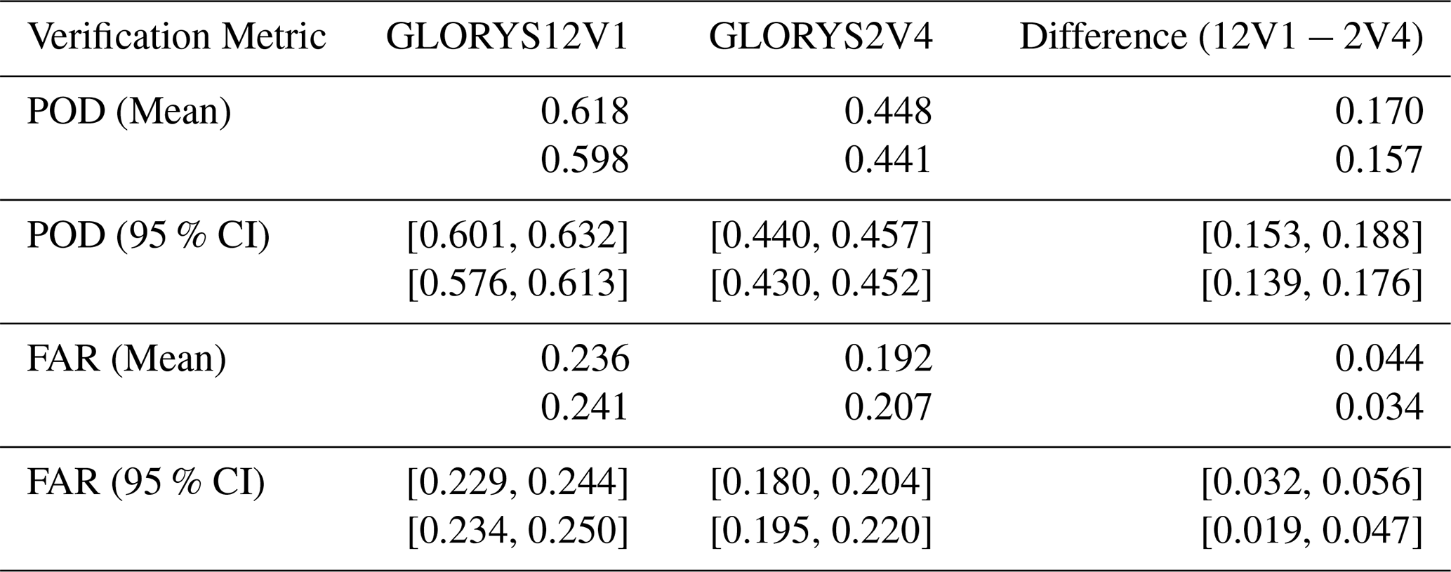
Sensitivity of verification metrics to eddy amplitude thresholds

To assess the sensitivity of the verification results to eddy amplitude, POD and FAR were recomputed using minimum amplitude thresholds of 5, 10, 15, and 20 cm. We also considered the complementary subset of eddies with amplitudes lower than or equal to 10 cm to isolate the contribution of low-amplitude features. The 10 cm value is used only as a diagnostic criterion and not as a physical boundary between different eddy regimes.

The verification metrics do not improve monotonically as low-amplitude eddies are progressively excluded. For GLORYS12V1, POD remains approximately between 0.58 and 0.62, while FAR remains between about 0.27 and 0.31. For GLORYS2V4, POD is approximately 0.46–0.47 at the 5 cm threshold and decreases to approximately 0.36–0.37 at 20 cm, while FAR increases from approximately 0.37–0.38 to approximately 0.45. The higher thresholds also retain fewer eddies, producing larger day-to-day variability. Therefore, these results do not indicate a uniform improvement in the representation of stronger eddies.

For higher amplitude thresholds, the metric values show much larger variations over time. On some days, the POD values are close to 1 and the FAR values are close to 0, while on other days they are much farther from these ideal values. This variability is mainly caused by the smaller number of eddies with amplitudes above 10 or 20 cm. For this reason, the POD and FAR time series can show large variations and can rapidly move towards values close to 0 or 1. These results suggest that the imperfect matching between the reanalyses and the observational datasets mainly concerns small ocean eddies. However, this improvement does not mean that the complete eddy field is better represented.

As the minimum amplitude threshold increases, the absolute numbers of both hits and misses decrease because fewer eddies satisfy the criterion. For GLORYS12V1, the mean number of hits remains higher than the number of misses at all thresholds. For GLORYS2V4, misses remain more numerous than hits and their relative importance increases at higher thresholds. This behaviour is consistent with the reduction in POD observed for GLORYS2V4. The power spectra in Fig. C2 show that temporal variability generally increases with the minimum amplitude threshold, mainly at longer periods, while differences remain limited at short periods. GLORYS12V1 generally shows larger POD spectral peaks, whereas GLORYS2V4 generally shows larger FAR peaks, with exceptions at 15 cm for POD and 5 cm for FAR. Figure C3 shows that both hits and misses decrease in absolute number as the threshold increases because fewer eddies are retained. However, GLORYS12V1 maintains more hits than misses, whereas misses remain more numerous than hits for GLORYS2V4, indicating a greater reduction in matching performance for GLORYS2V4 at higher amplitude thresholds. We also evaluated POD and FAR for low-amplitude eddies (≤ 10 cm), whose weak SSH signatures make their detection and matching more sensitive to mapping, filtering, and background variability. This subset is therefore expected to show lower POD and higher FAR because small differences between observational and reanalysis fields can alter eddy position and contours or generate unmatched features.

Figure C5 shows the distributions of hits, misses, and false alarms as functions of eddy radius and amplitude.

We further introduce the histograms of the eddy matching statistics, namely hits, misses, and false alarms, as a function of both eddy radius and eddy amplitude. The aim is to provide a more detailed view, similar to a zoomed-in analysis, of how the matching statistics vary with the two main physical eddy features. This additional representation is useful because, on a linear scale, the histograms are not always able to clearly show the distinct behaviour of each matching statistic as eddy amplitude and radius increase. A logarithmic y-axis is used to distinguish the matching categories in bins containing fewer eddies. This is shown in Fig. C5.

At the smallest radii and amplitudes, misses are particularly prominent, especially for GLORYS2V4, confirming its greater difficulty in representing small eddies. GLORYS12V1 produces more hits in these classes, although this is accompanied by more small false alarms. For eddy radius, GLORYS2V4 has more misses than GLORYS12V1 up to approximately 150 km, while its false alarms become more numerous above about 50 km. In the amplitude distributions, misses remain the main source of error for GLORYS2V4. Above radii of approximately 50 km and amplitudes of 8–10 cm, hits become the dominant category for both reanalyses and both observational references. The largest discrepancies are therefore concentrated among smaller and lower-amplitude eddies.

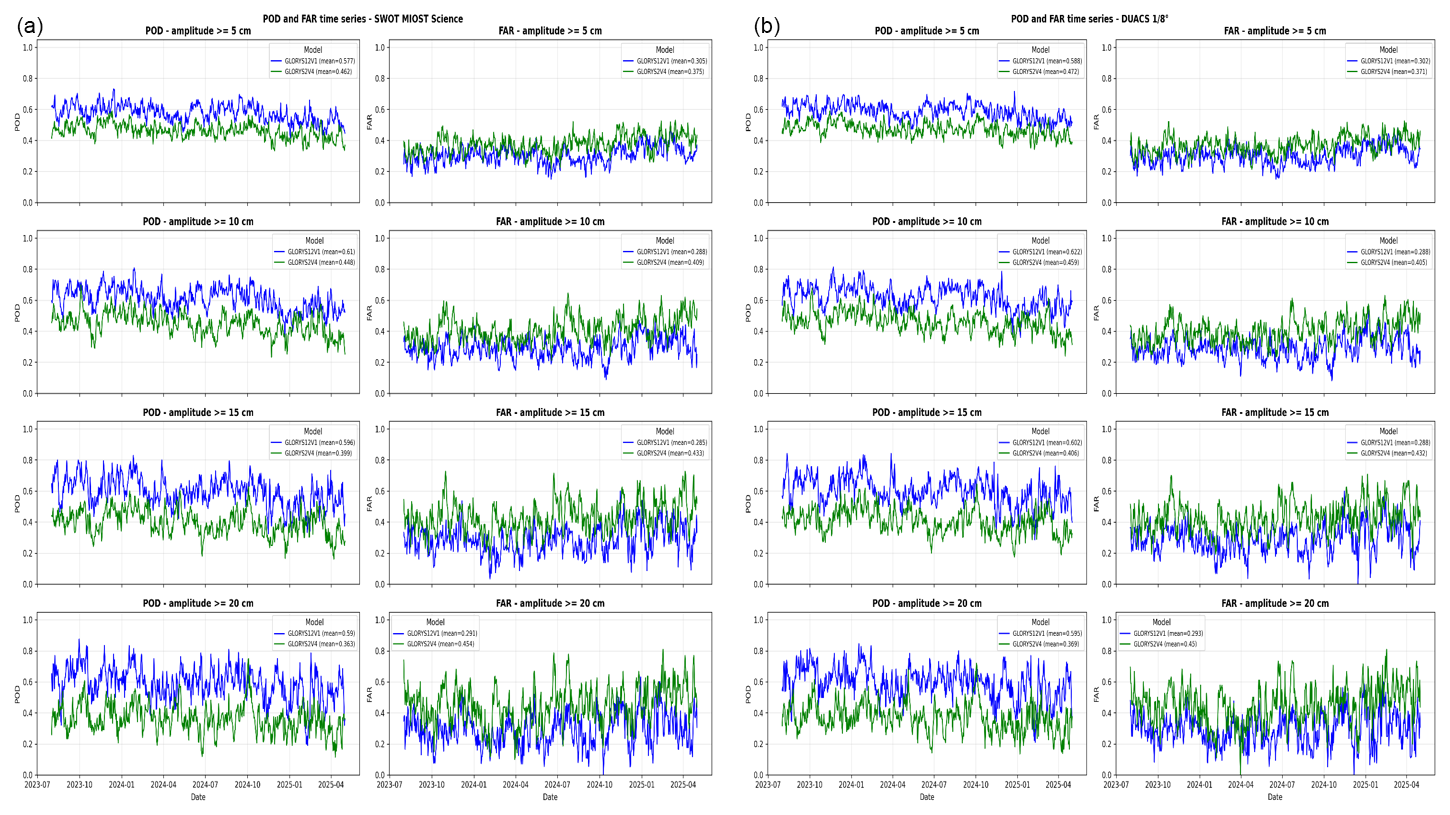
Figure C1 Time series for POD & FAR by amplitude threshold: 5, 10, 15, 20 cm, for SWOT comparison (a) and for DUACS $\mathrm{1}/\mathrm{8}$° comparison (b), with a minimum lifetime threshold of 4 d.

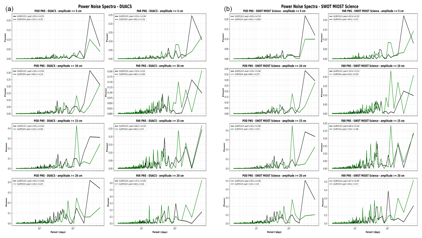
Figure C2 Power spectra of the POD and FAR time series for each reanalysis product for the (a) DUACS and (b) SWOT MIOST Science comparisons. Agreement does not improve consistently when progressively higher minimum-amplitude thresholds are applied. GLORYS2V4 shows a clear increase in FAR at the highest thresholds.

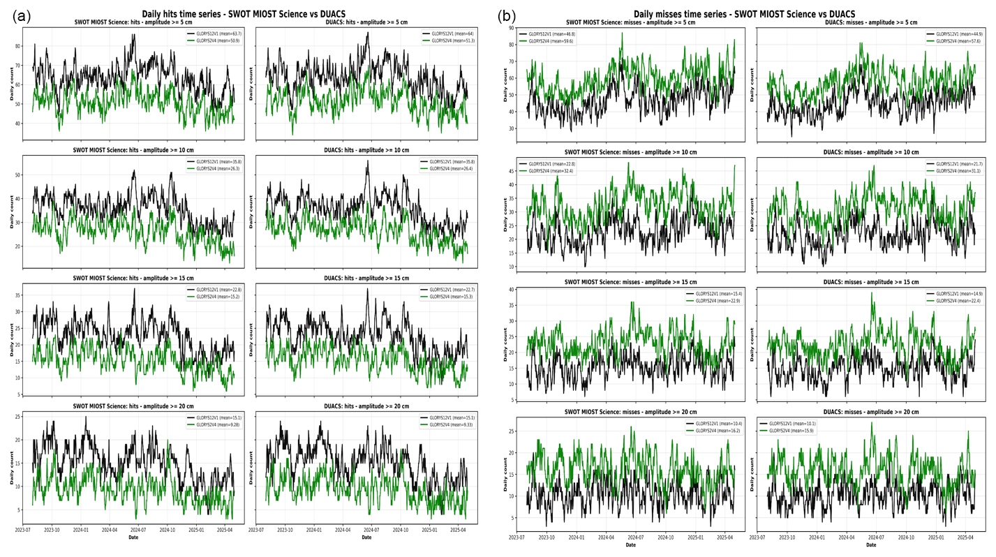
Figure C3 Time series of the daily numbers of (a) hits and (b) misses for the two satellite datasets compared with the reanalyses. The left panels show SWOT MIOST Science, and the right panels show DUACS.

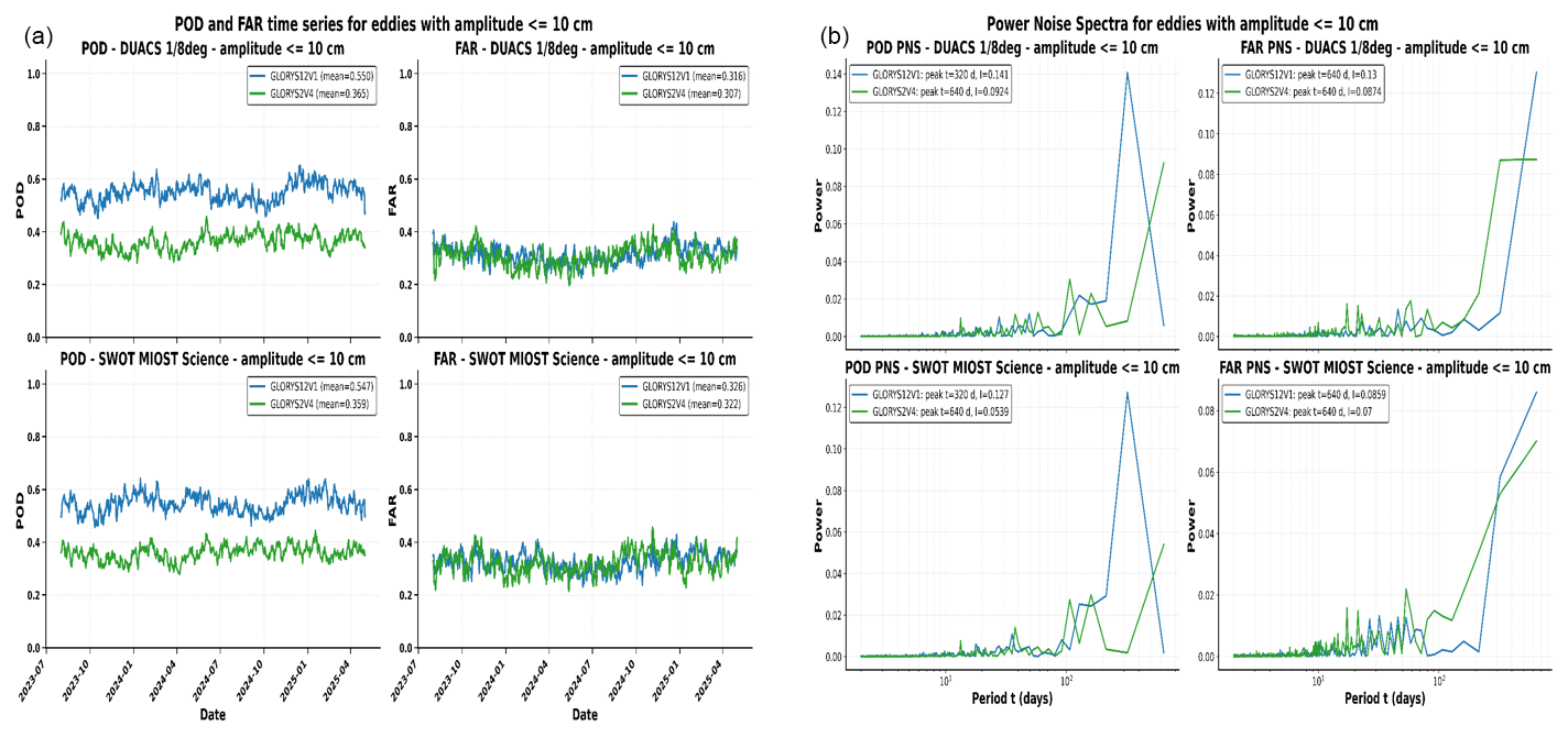
Figure C4 (a) POD and FAR time series for eddies with amplitudes ≤ 10 cm for the comparisons with DUACS $\mathrm{1}/\mathrm{8}$° and SWOT MIOST Science. (b) Corresponding power spectra. A 4 d minimum-lifetime threshold is used.

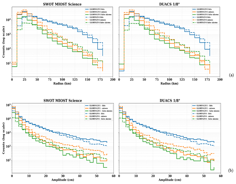
Figure C5 Histograms for eddy matching statistics on a logarithmic scale, for both comparisons, for eddy radius (a) and eddy amplitude (b).

Appendix D

This appendix assesses the sensitivity of the verification results to two methodological choices: (i) the maximum centroid distance allowed in the eddy-matching procedure and (ii) the cutoff wavelength of the Bessel high-pass filter applied before eddy detection. The reference values are 125 km for the matching distance and 500 km for the filter cutoff wavelength. The alternative values tested here are 62.5 km for matching and 200 and 800 km for filtering. All other methodological settings, including the 4 d minimum lifetime threshold, remain unchanged.

D1 Sensitivity to the eddy-matching distance threshold (62.5 km)

The matching analysis was repeated using a maximum centroid distance of 62.5 km, corresponding to half of the reference value of 125 km. This more restrictive criterion allows only eddies with closer centroid positions to be matched. When a pair accepted with the 125 km threshold no longer satisfies the 62.5 km criterion, the reference eddy is classified as a miss and the corresponding reanalysis eddy as a false alarm.

Figure D1 shows an example for anticyclonic eddies on 1 January 2025. The stricter threshold reduces the number of hits and increases both misses and false alarms, demonstrating the sensitivity of the matching statistics to the maximum distance allowed between eddy centroids.

The verification metrics are computed on a daily basis, following the same procedure described in Sects. 2.4 and 3.2, in order to evaluate the temporal evolution of the matching performance. Tables D1 and D2 report the absolute and relative changes in the verification metrics for the two comparisons, respectively.

Overall, when the maximum matching distance is reduced from 125 to 62.5 km, FAR becomes higher for GLORYS2V4 than for GLORYS12V1, as shown in Tables D1, D2, Figs. D1 and D2a. This does not necessarily mean that GLORYS2V4 produces a larger absolute number of false alarms. Rather, it reflects the relative nature of FAR, which depends on the proportion of unmatched reanalysis eddies with respect to the total number of reanalysis detections considered in the verification.

In contrast, POD remains higher for GLORYS12V1, indicating that the higher-resolution reanalysis is still able to match a larger fraction of the observed eddies, even under the more restrictive distance criterion. The most evident effect of reducing the matching distance is the strong increase in FAR, especially for GLORYS2V4, where FAR more than doubles in both satellite-based comparisons. A substantial increase is also found for GLORYS12V1, with FAR increasing by more than 70 %. POD also decreases when the reduced distance threshold is applied, but the relative reduction is smaller than for FAR. The decrease is of the order of 20 % for GLORYS12V1 and about 30 % for GLORYS2V4. This indicates that the reduced distance threshold may affect the classification of unmatched reanalysis detections, leading to a large increase in false alarms, while the reduction in correctly matched observed eddies is less pronounced.

The power spectra in Fig. D2b show slightly larger main POD peaks for GLORYS2V4 than for GLORYS12V1. In the SWOT comparison, the main POD peaks occur at approximately 71 d for GLORYS2V4 and 128 d for GLORYS12V1, whereas both are located near 107 d in the DUACS comparison. The strongest FAR peaks occur at longer resolved periods. Because the evaluation period is only approximately 640 d long, peaks at or near 640 d should be interpreted as low-frequency variability rather than as evidence of a robust periodic cycle.

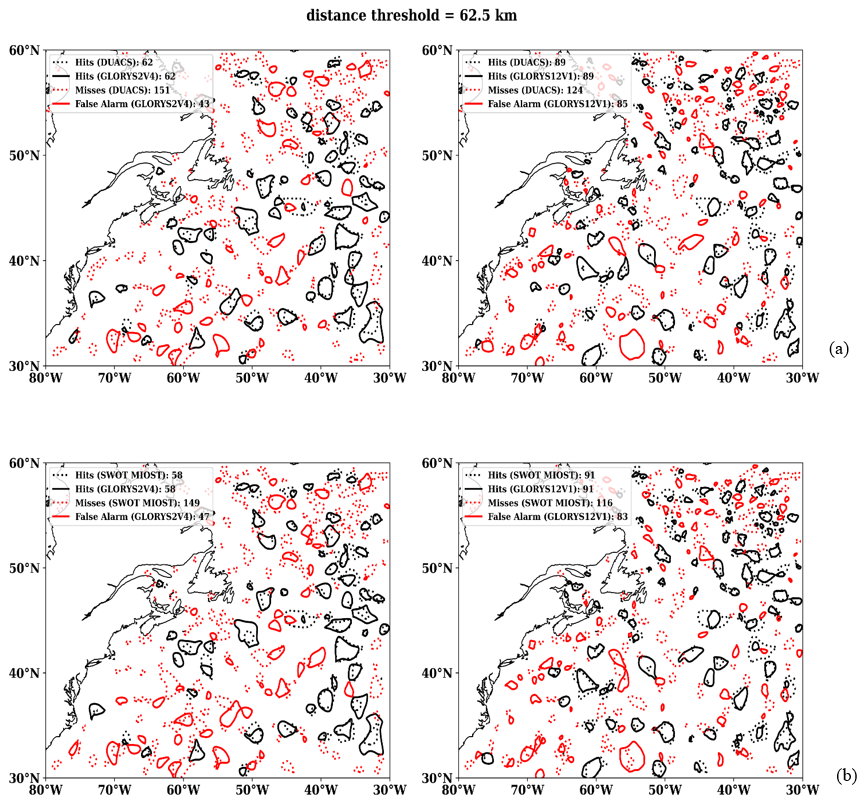
Figure D1 Anticyclonic-eddy matching on 1 January 2025 using a maximum centroid distance of 62.5 km. GLORYS2V4 is shown on the left and GLORYS12V1 on the right, for the comparisons with (a) DUACS $\mathrm{1}/\mathrm{8}$° and (b) SWOT MIOST Science.

Table D1 Aggregated eddy verification statistics for the Probability of Detection (POD) and False Alarm Ratio (FAR) for the comparison with SWOT using maximum matching distances of 125 and 62.5 km. Absolute and percentage differences are calculated as the 62.5 km result minus the 125 km result.

Table D2 Aggregated eddy verification statistics for the Probability of Detection (POD) and False Alarm Ratio (FAR) for the comparison with DUACS using maximum matching distances of 125 and 62.5 km. Absolute and percentage differences are calculated as the 62.5 km result minus the 125 km result.

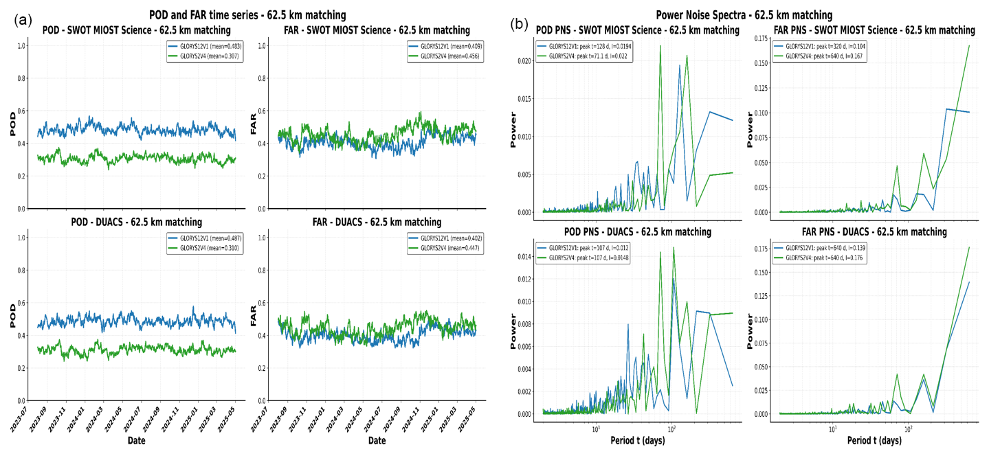
Figure D2 (a) Time series of the verification metrics for the comparisons with SWOT MIOST Science and DUACS 1/8°, using a 4 d minimum-lifetime threshold. (b) Power spectra of all time series shown in panel (a).

D2 Sensitivity to the Bessel-filter cutoff used in the eddy-detection process

The SSH or ADT fields of all products were high-pass filtered using a Bessel filter before eddy detection. The reference cutoff wavelength is 500 km. To assess the sensitivity of the detection and verification results to the retained spatial scales, the complete detection, tracking, and matching procedure was repeated using cutoff wavelengths of 200 and 800 km. The 200 km cutoff applies more restrictive spatial filtering, whereas the 800 km cutoff retains a broader range of large-scale variability.

Reducing the Bessel-filter cutoff wavelength from 500 to 200 km increases POD and decreases FAR for both reanalyses and both observational comparisons. The changes are particularly pronounced for GLORYS2V4, for which POD increases by approximately 18 % and FAR decreases by approximately 34 %–35 %. For GLORYS12V1, POD increases by about 8 %–9 % and FAR decreases by approximately 17 %–18 %. Increasing the cutoff wavelength from 500 to 800 km produces smaller and opposite changes: POD decreases and FAR increases for both reanalyses. The POD reduction is larger for GLORYS2V4, whereas the FAR changes remain relatively small. For both cutoff tests, POD is slightly more sensitive in the SWOT comparison, while FAR is generally more sensitive in the DUACS comparison. These changes show that the verification metrics depend on the spatial scales retained before eddy detection. However, the better verification scores obtained with the 200 km cutoff wavelength do not necessarily demonstrate that this value is physically more appropriate, because stronger filtering may remove structures that would otherwise remain unmatched. Regarding the power spectra, the largest peaks for POD are observed for GLORYS12V1 using the 200 km filter cutoff, at temporal scales of the order of several hundred days, approximately 320 d. For FAR, the highest values are instead found for GLORYS12V1 with the 800 km filter cutoff, with enhanced power around 640 d. At shorter temporal scales, the variability is similar across all datasets and filter configurations. Overall, in terms of spectral power, the strongest peak is found for the POD of GLORYS12V1 with the 200 km filter cutoff in the comparison with SWOT MIOST.

Table D3 Mean eddy-verification metrics and their absolute and percentage changes when the Bessel-filter cutoff wavelength is reduced from 500 to 200 km for both comparisons.

Table D4 Mean eddy-verification metrics and their absolute and percentage changes when the Bessel-filter cutoff wavelength is increased from 500 to 800 km for both comparisons.

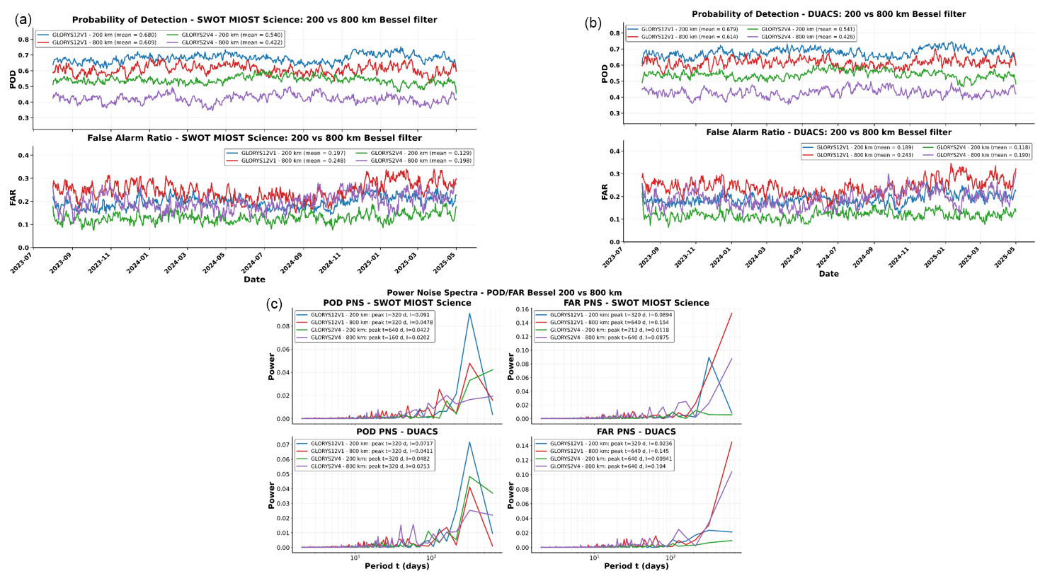
Figure D3 POD and FAR time series obtained using Bessel-filter cutoff wavelengths of 200 and 800 km for the comparisons with (a) SWOT MIOST Science and (b) DUACS $\mathrm{1}/\mathrm{8}$°. Panel (c) shows the corresponding power spectra. A 4 d minimum-lifetime threshold is used.