An improvement to short term variability in Global Mean Sea Level reconstruction

We hypothesise that there is an overestimation of Global Mean Sea Level (GMSL) variability from GMSL empirical orthogonal function (EOF) reconstructions due to differences between the tide gauge observations and their corresponding altimetry data. We show that these differences are correlated well with local winds along coastlines, suggesting that observations from tide gauges at the coast and satellite altimetry near the coast could partially be explained by the wind forcing. Correcting these differences through a mainly wind-driven regression model prior to the EOF reconstruction, reduces the standard deviation (SD) of the reconstructed GMSL variability by 23 % and significantly increases the correlation to 0.40 with respect to the observed averaged GMSL calculated from altimetry grid points (1994 to 2020). The model was used to extrapolate these differences prior to 1993 and a corrected GMSL reconstruction is presented.

1 Introduction

Global Mean Sea level (GMSL) changes are primarily the result of ocean heat uptake and ice mass loss from glaciers and ice sheets. Consequently, measuring GMSL has become an important factor to assess the health of the world's climate, by providing observational evidence of climate system response to the warming of the planet due to increased greenhouse gases (IPCC, 2021). The GMSL variability is a fundamental part in understanding the sea level budget, for example, the contributions of ice mass loss from glaciers and warming of the ocean for individual years/decades. Satellite observations that include GRACE (ocean mass) and altimetry have provided a major tool in understanding mechanisms such as ocean warming and land ice melt by studying the sea level budget (WCRP Global Sea Level Budget Group, 2018). However, GMSL has only been observed directly through satellite altimetry since late 1992. Prior to this, measurements of sea level come primarily from tide gauges and, thus, are restricted to coastal locations. Therefore, there is a need to improve the GMSL variability estimates prior 1993.

One of the most widely used methods to produce global sea level reconstructions for the pre-altimetry era is the reduced space optimal interpolation (RSOI) technique (Kaplan et al., 1997, 2000). This technique involves inferring empirical orthogonal functions (EOFs) from altimetry data and then fitting a subset of those to tide gauge records to estimate the temporal amplitude associated with each EOF. A spatially uniform EOF (often called EOF0) is typically added to the subset of original EOFs, as first proposed by Church et al. (2004), because otherwise the long-term trends are not adequately reconstructed. We refer to such reconstructions as EOF reconstructions. Other examples of these reconstructions include Church and White (2006), Church and White (2011); Mu et al. (2018); Ray and Douglas (2011); and Strassburg et al. (2014). Recently, Wang et al. (2024) expanded the EOF technique of Church and White (2011) by incorporating barystatic-GRD (gravitational, rotational, and deformation) fingerprints and sterodynamic sea-level patterns, which allowed them to dispense with the EOF0.

Past studies have shown that, while including an EOF0 significantly improves the estimation of the underlying long-term trend in GMSL, it comes at the cost of losing the ability to reconstruct the interannual to decadal variability (Calafat and Gomis, 2009; Calafat et al., 2014). To illustrate this issue, we show a comparison between detrended de-seasoned “true” GMSL from the gridded global CMEMS altimetry product (a simple global average per time step) and the GMSL EOF reconstruction from Church and White (2011; hereinafter CW11) updated to include data up to 2013 (Fig. 1). The two time series show little resemblance with a correlation of −0.19. Furthermore, the reconstructed GMSL overestimates the variability by a factor of more than two (SDs of 0.45 and 0.21 cm for the reconstruction and the true GMSL observations, respectively). An accurate representation of the variability in GMSL is important, not only because it reveals useful information on the global hydrological cycle (Llovel et al., 2011), but also because it influences the estimation of underlying long-term trends and accelerations in GMSL. Hamlington et al. (2020b) examined the steric and barystatic contributions to interannual to decadal variability in GMSL back to 1982 and found that both are highly correlated with the ENSO variations and contribute equally to observed GMSL variability. Sea level variability is becoming increasingly significant as it contributes to coastal flooding and erosion (Widlansky et al., 2020).

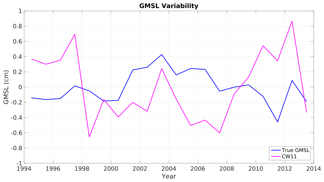
Figure 1 The true GMSL variability from CMEMS altimetry and an updated dataset CW11 (Church and White, 2011) for the period 1994 to 2013.

Noting the issues that arise when including an EOF0, some studies have developed hybrid sea-level reconstructions where the variability is derived from EOF reconstructions without the EOF0 whereas the trends are estimated using other methods such as Bayesian fingerprinting (Dangendorf et al., 2019, 2021, 2023). Such hybrid reconstructions appear to produce good estimates of both the variability and the underlying trends, but they also come with challenges compared to using a unified statistical method, such as potential distortions in the reconstructed time series if the two components do not integrate well and also increased complexity. In this study, we explore ways of improving the estimation of the GMSL variability in EOF reconstructions that include the EOF0.

While the sparseness of the tide gauge data in time and space is likely to affect the skill of EOF reconstructions (Calafat and Gomis, 2009; Calafat et al., 2014; Christiansen et al., 2010; Natarov et al., 2017), it alone does not explain why EOF reconstructions with an EOF0 fail to capture the GMSL variability. We know this because reconstructions that do not include an EOF0 are able to capture the variability in GMSL with relatively good accuracy. Indeed, Calafat et al. (2014) showed, based on a series of numerical experiments, that the low skill of EOF reconstructions (with an EOF0) to capture the short-term GMSL variability is largely due to differences between tide gauges and the corresponding altimetry point. Such differences arise mainly due to the degradation of the satellite altimetry data within ∼ 10–20 km of the coast (Cipollini et al., 2017). Calafat et al. (2014) showed that if the tide gauges in an EOF reconstruction are replaced by the corresponding altimetry points (i.e., altimetry coastal points are used as virtual tide gauges), effectively removing any differences between tide gauges and altimetry, the variability in GMSL is well captured even when including an EOF0. This demonstrates the crucial role that differences between tide gauges and altimetry play in the reduced skill of EOF reconstructions.

With a view of improving the skill of EOF reconstructions that include an EOF0, we investigate the nature of the differences between the tide gauge and altimetry signals (hereafter referred to as Signal Differences). We show that such differences have a coherent spatial structure along the coast, suggesting a geophysical origin as opposed to being caused by random errors. Further, we show that the Signal Differences are significantly correlated with wind variability. This allows us to model the Signal Differences at each tide gauge site through linear regression for the whole period of the reconstruction (using wind data from reanalyses) and subtract them from the tide gauge data prior to using them in an EOF reconstruction. We show that this leads to an improved reconstruction of the GMSL variability (1941 to 2020).

2 Data and Methods

2.1 Tide Gauge data

Monthly mean values of sea level from tide gauge records were obtained from the Permanent Service for Mean Sea Level (PSMSL) archive (Permanent Service for Mean Sea Level, 2023; Holgate et al., 2013). For consistency, we use the same tide gauge stations as those used in the CW11 reconstruction. Note that these include both Revised Local Reference (RLR) data and Metric data. In particular, a total of 602 tide gauges were used in the reconstruction, consisting of 491 RLR records (81.6 %) and 111 Metric records (18.4 %) starting from 1901.

The monthly tide gauge data had the PSMSL quality control flags applied before the annual and semi-annual cycles were removed by harmonic analysis over the entire period covered for each tide gauge record. The monthly tide gauge records were then corrected for Glacial Isostatic Adjustment (GIA) using the ICE5Gv1.3 (VM2_L90_2012) model for the relative sea level (Peltier, 2004). These GIA values are available on the PSMSL website (Peltier, 2026). The tide gauge data were also adjusted for atmospheric pressure changes using the inverse barometer (IB) approximation. The atmospheric pressure data were obtained from the 20th Century reanalysis (Compo et al., 2011) for the period 1901–1947 and from the NCEP/NCAR reanalysis (Kalnay et al., 1996) for the period 1948–2020. To merge the two atmospheric pressure datasets and ensure their consistency, we forced the two products to have the same time-mean pressure over their overlapping period (1948–2012). For further quality control, each tide gauge record was visually inspected. If any datum shifts were suspected within the time series, then the record in question was compared with records from nearby stations to confirm validity. If a shift was detected and confirmed, then the tide gauge record was split into segments and treated separately. A second pass for each monthly tide gauge record was carried out, removing any observations that were five SDs from the mean. This was to ensure that outliers were removed. A total of 36 values were removed from the entire dataset during this process.

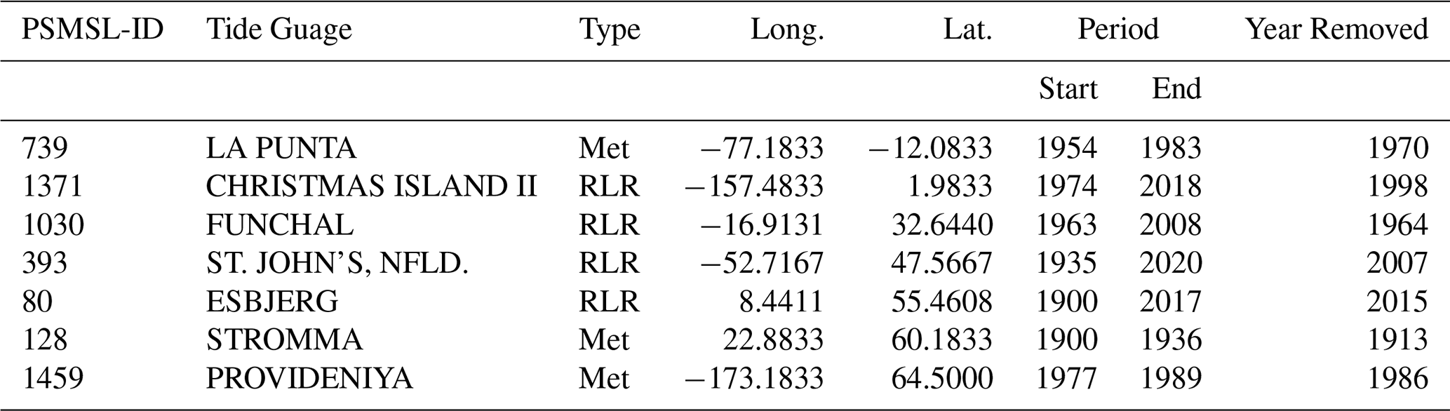
The monthly tide gauge records were then averaged into yearly values, where a requirement of having at least seven months of observations within the same year was imposed. Following CW11, each record was then differentiated in time using first differences between adjacent years (hereafter denoted by successive differences), effectively placing all the tide gauge records on the same vertical reference frame. We note that the reconstruction method works with successive differences rather than sea level observations; this is to accommodate the fact that tide gauge observations are using different datums. Any yearly successive differences greater than 0.25 m were removed. This value was chosen to ensure that no yearly value accidentally straddled a datum shift of monthly values within the same year. A total of seven yearly observations were removed (one year removed from each of seven individual tide gauge stations) over the entire dataset during this procedure (Table 1).

Table 1 Tide gauges from the PSMSL dataset that had one year removed (Year Removed) where their successive differences observations exceeded 0.25 m. The Start and End Period of each tide gauge time series are shown. Please Note, that the overall tide gauge dataset period is from 1900 to 2020. Type gives the PSMSL classification of Revised Local Reference (RLR) or Metric (Met).

Following CW11, the quality-controlled tide gauge stations are spatially averaged (combined) into 1° × 1° grouped tide gauge bins time series for a total of 285 tide gauge bins. In detail, the number of tide gauge stations can vary between tide gauge bins, which includes overlapping or different temporal coverages. However, for each 1° × 1° bin the individual time steps, comprising of observations of successive differences, are averaged. The composite tide gauge time series are then ready for the EOF reconstruction. The spatial and temporal distribution of the PSMSL tide gauge stations and the composite dataset using tide gauge bins are displayed in Fig. 2.

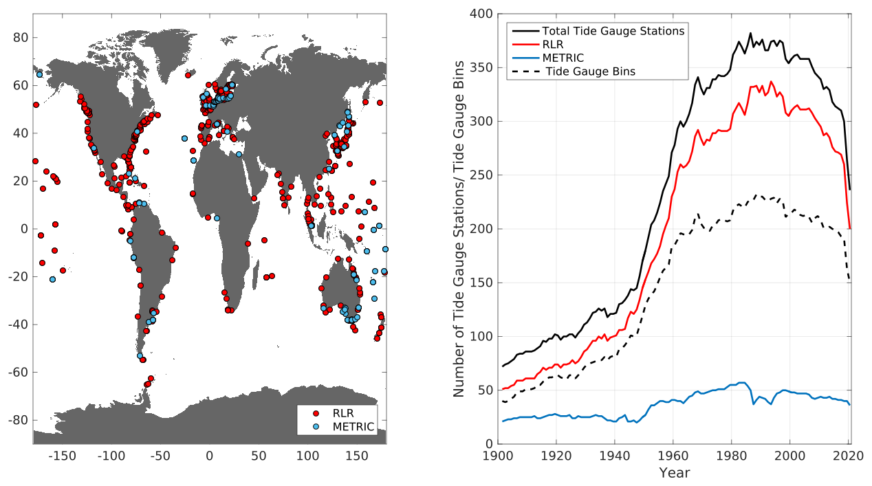
Figure 2 The spatial and temporal distribution of the number of tide gauges used in this study (1901–2020). The dashed black line represents the temporal distribution of the tide gauge bins containing composite tide gauge observations for the EOF GMSL reconstruction.

2.2 Altimetry dataset

In this study, we use a multi-mission gridded ($\frac{\mathrm{1}}{\mathrm{4}}$° resolution) weekly sea surface height product (SEALEVEL_GLO_PHY_L4_MY_008_047) from the Copernicus Marine Environment Monitoring Service (CMEMS; available at http://marine.copernicus.eu/, last access: 26 September 2022) spanning the period 1993 to 2020. The altimetry data had the annual and semi-annual cycles removed using harmonic analysis and the Peltier's GIA correction (Peltier, 2004). We applied the geoid-only GIA correction, obtained as the sum of the GIA-induced relative sea level change and the vertical motion of the solid earth due to GIA (dsea250.1grid.ICE5Gv1.3_VM2_L90_2012 + drad250.1grid.ICE5Gv1.3_VM2_L90_2012 dataset, Peltier, 2026). The altimetry data also had all the standard geophysical corrections applied, including the IB correction.

In summary, the GIA correction applied to tide gauge and altimetry are shown in Eq. (1).

$$\begin{array}{}\text{(1)}& \begin{array}{rl}& \mathrm{Tide}{\mathrm{Gauge}}_{{\mathrm{GIA}}_{\mathrm{corr}}}=\mathrm{Tide}\mathrm{Gauge}\mathrm{Obs}-{\mathrm{GIA}}_{\mathrm{corr}}\left(\mathrm{drsl}\mathrm{250}\right).\mathrm{\Delta }t\\ & {\mathrm{Altimetry}}_{{\mathrm{GIA}}_{\mathrm{corr}}}=\mathrm{Altimetry}\mathrm{Obs}-{\mathrm{GIA}}_{\mathrm{corr}}\left(\mathrm{dsea}\mathrm{250}+\mathrm{drad}\mathrm{250}\right).\mathrm{\Delta }t\end{array}\end{array}$$

Where t denotes time, please note that the Peltier's GIA correction is in mm yr⁻¹.

The weekly CMEMS altimetry dataset was converted to yearly values at each $\frac{\mathrm{1}}{\mathrm{4}}$° grid cell. The individual tide gauge stations within each tide gauge bin were linked to the closest valid altimetry grid point within a search radius of 50 km. These altimetry points were then spatially averaged if there were more than one in the same bin, producing a subset of the original CMEMS dataset (hereafter referred as the altimetry CMEMS dataset), similar to the CW11 tide gauge binned locations (Fig. 3). All tide gauge stations within the tide gauge bin had a corresponding altimetry timeseries even if they shared the same altimetry pixel location. If this occurred, then they were treated as separate altimetry timeseries during the spatial averaging process. This would have a similar weighting effect to that of the corresponding spatially averaged tide gauge stations that were close to each other with a similar sea level signal.

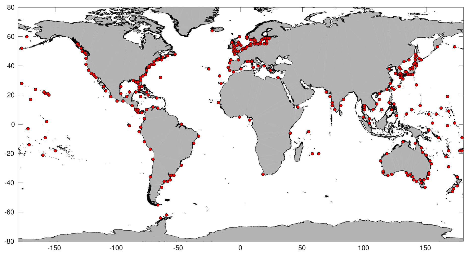
Figure 3 Distribution of the 285 tide gauge bins where the CMEMS altimetry data (1993 to 2020) coincides with binned tide gauge observations (1901 to 2020) that are used for our EOF reconstructions.

2.3 Wind dataset and Southern Oscillation Index

Previous work has shown that wind and climate indices play important roles in sea level variability, for example, Calafat et al. (2018); Han et al. (2017) and The Climate Change Initiative Coastal Sea Level Team (2020). Here, we aim to assess whether Signal Differences can be explained by wind forcing or climate indices. Because the EOF reconstruction is based on successive differences, this is what we use to define the Signal Differences rather than sea levels. For the wind analysis, we use monthly 10 m wind u and v components from the ERA5 reanalysis (Hersbach et al., 2023), which are provided at $\frac{\mathrm{1}}{\mathrm{4}}$° resolution and were downloaded from the Copernicus Climate Change Service, Climate Data Store website. The monthly wind data had the annual and semi-annual cycles removed using harmonic analysis at each grid point, and were then averaged in yearly values and detrended.

Wind u and v components were extracted within a 200 km radius from each individual tide gauge station. Successive differences were then applied to identify the grid point with the highest correlations between Signal Differences and the wind (u, v) timeseries. The wind (u, v) timeseries at the point of maximum correlation were then spatially averaged within each tide gauge bin and successive differences applied.

The second dataset was a climate index called the Southern Oscillation Index (SOI), a normalized pressure difference between Tahiti and Darwin (Ropelewski and Jones, 1987), which was downloaded from the University of East Anglia, Climatic Research Unit website. This dataset was yearly averaged and successive differences applied for consistency. The SOI was used as Calafat et al. (2014) commented that the El Niño–Southern Oscillation (ENSO) signal was not captured properly because the EOF0 was used in the GMSL reconstructions.

2.4 EOF Reconstruction

For simplicity, the term tide gauge bins hereinafter are referred to as tide gauges. Calafat et al. (2014) demonstrated that, in EOF reconstructions that include an EOF0, the reconstructed GMSL can be expressed as a generalized weighted mean of the tide gauge records.

$$\begin{array}{}\text{(2)}& \mathrm{GMSL}=\sum _{i=\mathrm{1}}^N{w}_i{t}_i\end{array}$$

where $w=\frac{{\mathrm{1}}^T{\sum }^{-\mathrm{1}}}{{\mathrm{1}}^T{\sum }^{-\mathrm{1}}\mathrm{1}}$ and ∑ is the covariance matrix of altimetry records at tide gauge locations and is diagonally loaded with the observational error. w_i is the weight associated with the ith tide gauge. N is the total number of tide gauges available at each time step i. 1 is an N × 1 column vector of ones.

This is the formulation that we use in this study, but we remark that such formulation is completely equivalent to that of CW11. Equation (2) is applied to annual data with an observational error of 2 cm.

As a sanity check, we reconstructed GMSL using the CMEMS global dataset (1993 to 2020) and tide gauges (Fig. 3) and compared it with the GMSL reconstruction of CW11 (Fig. 4). The trend from our GMSL reconstruction for the period 1901–2013 is 1.6 ± 0.1 mm yr⁻¹ whereas that from CW11's reconstruction is 1.7 ± 0.3 mm yr⁻¹, reflecting a very good agreement when considering their uncertainty estimates (which account for serial correlation). The two reconstructions agree also very well in terms of the variability with a correlation of 0.80 for detrended time series (1910 to 2013), although there is a small offset between the two GMSL curves between 1910 and 1950. If we expand the timeseries from 1901 to 2013 then the correlation is reduced to 0.55. The uncertainty (shaded region) is quite large from 1901 to 1910 compared with the later period of the GMSL reconstruction, so it is not surprising that the correlation had reduced between the two reconstructions. The uncertainty (±1σ) in the GMSL trends is estimated using a regression model with serial correlation errors, in order to obtain more realistic error estimates (Chib, 1993).

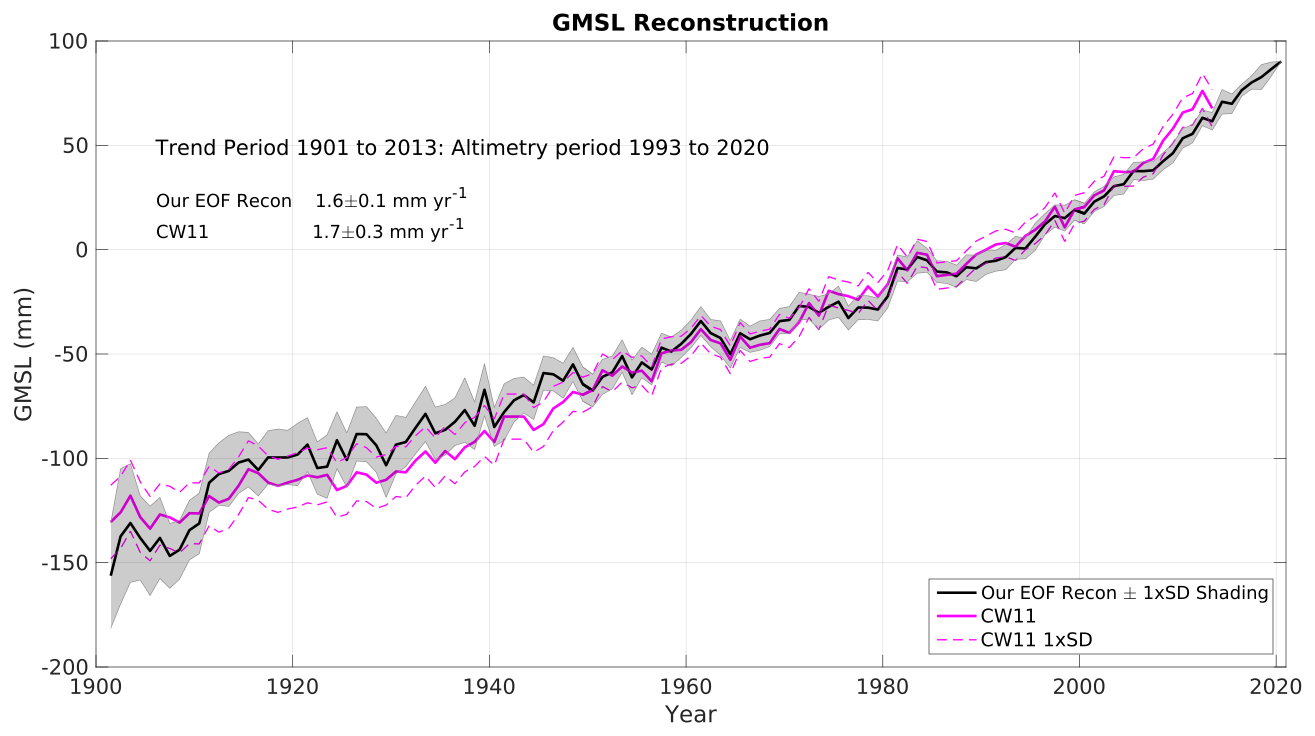
Figure 4 Comparison of our EOF reconstruction (black) derived from Eq. (2) with that of CW11 (magenta). The shaded area (grey) represent the 1-sigma uncertainty interval, which reflects the sensitivity of the reconstruction to the number of tide gauge bins as evaluated Standard deviation (SD) using a bootstrap method.

2.5 Multiple Linear Regression Model for Signal Differences

As discussed earlier, the low ability of EOF reconstructions to capture the GMSL variability appears to be largely due to differences between the tide gauges and the corresponding altimetry data (i.e., the Signal Differences). Hence, if we were able to build a regression model for the Signal Differences with good predictive skill, this would enable us to improve the reconstruction of the GMSL variability by adjusting the tide gauge data prior to the reconstruction which includes tide gauge observations before 1993. To this end, we will begin by investigating the relationship between the Signal Differences and plausible predictors such as wind, a climate index (Southern Oscillation Index) and the tide gauge record itself. The reason for including the tide gauge record as a predictor is to account for the possibility that the Signal Differences could be due to a simple scale factor between the altimetry and the tide gauge time series, or to local coastal signals unobserved by altimetry. To select the regression predictors, we performed an exploratory correlational analysis involving the Signal Differences and the plausible predictors listed above. Such analysis is based on detrended yearly timeseries with the successive differences applied.

Using these predictors, we designed three Signal Differences multiple linear regression models Eqs. (3) to (5) to be associated with each tide gauge. Model 1, Eq. (3) uses the wind u and v components as the predictors, followed by the addition of the SOI, Eq. (4) and tide gauge observation (TG, Eq. 5) sequentially. We tested the regression Models at each tide gauge by analyzing the correlations between the Signal Differences and the regression Models, and also their corresponding explained variance. It is important to note here these multiple regression models are designed to predict the Signal Differences rather than explaining their origin, thus we are not concerned whether the predictors are correlated.

$$\begin{array}{}\text{(3)}& {\displaystyle }\mathrm{Signal}{\mathrm{Differences}}_{\mathrm{Model}\mathrm{1}}=a+b_{\mathrm{1}}{\mathrm{Wind}}_u+b_{\mathrm{2}}{\mathrm{Wind}}_v\text{(4)}& {\displaystyle }\begin{array}{rl}\mathrm{Signal}{\mathrm{Differences}}_{\mathrm{Model}\mathrm{2}}& =a+b_{\mathrm{1}}{\mathrm{Wind}}_u\\ & +b_{\mathrm{2}}{\mathrm{Wind}}_v+b_{\mathrm{3}}\mathrm{SOI}\end{array}\text{(5)}& {\displaystyle }\begin{array}{rl}\mathrm{Signal}{\mathrm{Differences}}_{\mathrm{Model}\mathrm{3}}& =a+b_{\mathrm{1}}{\mathrm{Wind}}_u\\ & +b_{\mathrm{2}}{\mathrm{Wind}}_v+b_{\mathrm{3}}\mathrm{SOI}+b_{\mathrm{4}}\mathrm{TG}\end{array}\end{array}$$

3 Results

We start by comparing our uncorrected GMSL reconstruction with the “true” GMSL from altimetry for the period 1994 to 2020 (Fig. 5). The variability in the two time series is fairly different, with a correlation of 0.20. The SD of our reconstruction was 0.30 cm and that of the “true” GMSL was 0.25 cm. Next, we compute a second GMSL reconstruction by replacing the tide gauges with the corresponding altimetry time series (virtual altimetric tide gauges). Note that in this second reconstruction, the Signal Differences are exactly zero by construction. In this case, the GMSL reconstruction is almost a perfect match to the “true” GMSL variability (Fig. 5), with a correlation of 0.98. These results strongly support the statement that we made in the Introduction that differences between tide gauges and the corresponding altimetry data lead to a significant shortfall in the skill of EOF reconstructions that include an EOF0. They also suggest that we can potentially improve the skill of the EOF reconstructions by adjusting such differences prior to conducting the reconstruction.

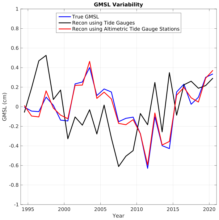
Figure 5 Comparison between the true GMSL and our GMSL reconstructions using tide gauge observations (black line) and virtual altimetric tide gauges (red line) for the period 1994 to 2020. The “true” GMSL derived from altimetry is shown as a blue line. All timeseries are detrended.

The next stage of this study is to investigate if these Signal Differences have any spatial structure that can be exploited to build a regression model of the Signal Differences. This would then allow us to remove the Signal Difference from the tide gauge data, potentially leading to a better GMSL reconstruction.

3.1 Signal Differences

Recall that the Signal Differences are defined as the difference between each binned tide gauge location and its corresponding binned altimetry observations where both the tide gauge and altimetry data had the successive differencing applied.

We begin by showing the SD of the Signal Differences for the period 1994 to 2020 using 229 tide gauges (Fig. 6). The original 285 locations from the tide gauge dataset were subsampled to 229 locations where the data covered at least eight years, so that we could maximize the number of locations to estimate reliable correlations and SDs of the Signal Differences. Of the 229 locations in the subsample, most (90 %) contained at least 16 years of data.

Figure 6 The Standard Deviation (SD) of the Signal Differences.

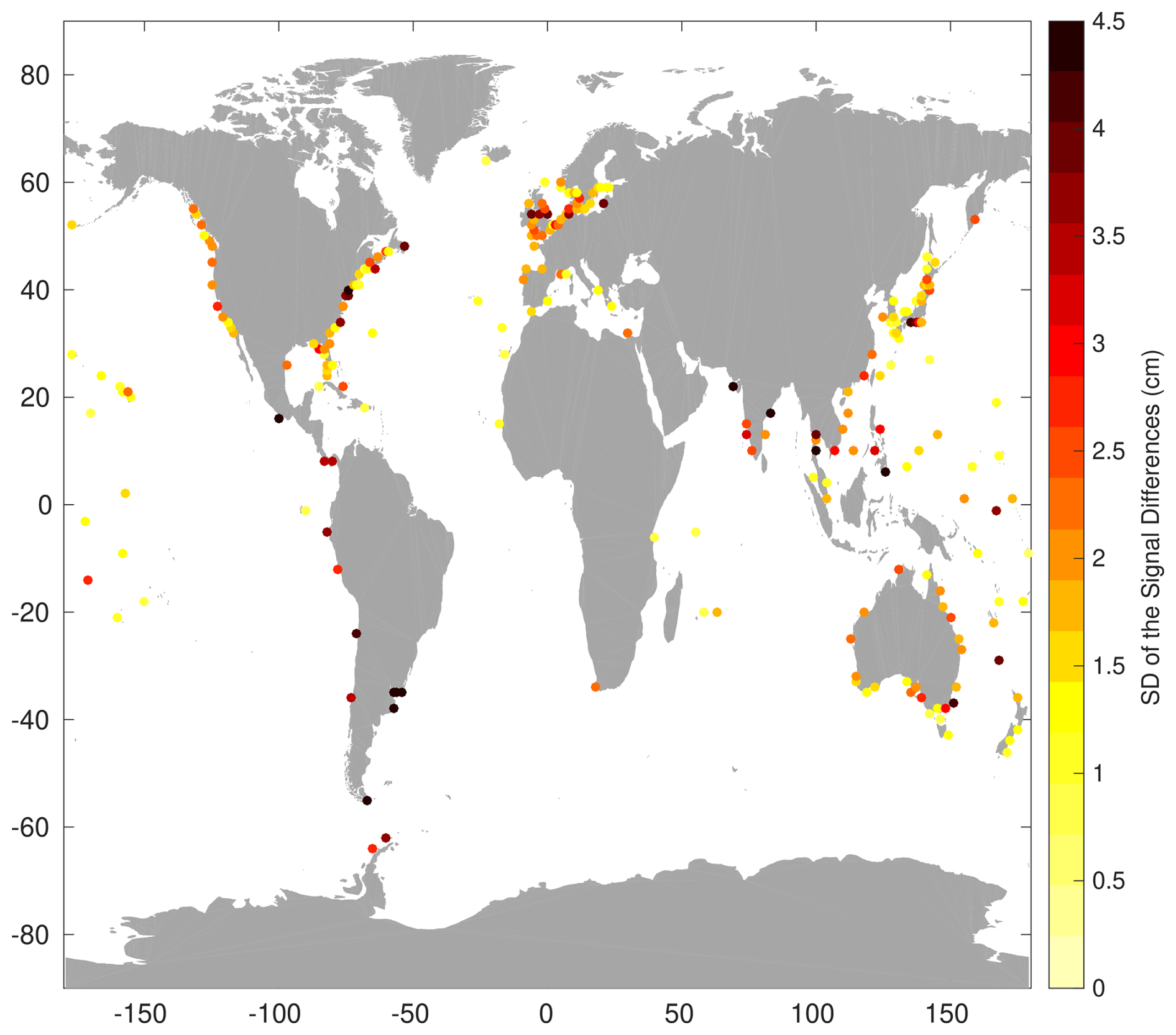
The spatial distribution of the Signal Differences shows SD values ranging from almost 0 to 4.5 cm where clusters of medium to high values (> 2 cm) are generally found along continental coastlines and low values (< 1.5 cm) found along both continental coastlines and islands within the open ocean (Fig. 6). This provides some evidence of spatial structure (coherency) within the Signal Differences data. To further quantify the coherence of the Signal Differences, we correlate the Signal Differences from individual sites with the average of the Signal Differences over all sites within four different regions, namely the west coast of North America, the Bay of Biscay/English Channel, North East Australia, and South America (Fig. 7). The average correlation for each region is, respectively 0.68 (SD 0.15), 0.74 (SD 0.11), 0.65 (SD 0.08) and 0.62 (SD 0.12). The correlation values are not completely uniform within each region, but this is likely due to unique localised physical mechanisms (such as bathymetry; local vertical movement; ocean currents; wind; etc.) that may affect these differences between the tide gauge and altimetry observations. These correlations are high enough to conclude that the Signal Differences are not random but rather due to coastal signals not captured by altimetry and/or a scale factor between the tide gauge and altimetry measurements. Indeed, if we replace all the Signal Differences in Fig. 7a (i.e. 7 tide gauges) with random values and repeat the analysis 100 000 times, then the mean correlation is 0.37, much lower than what we find in reality.

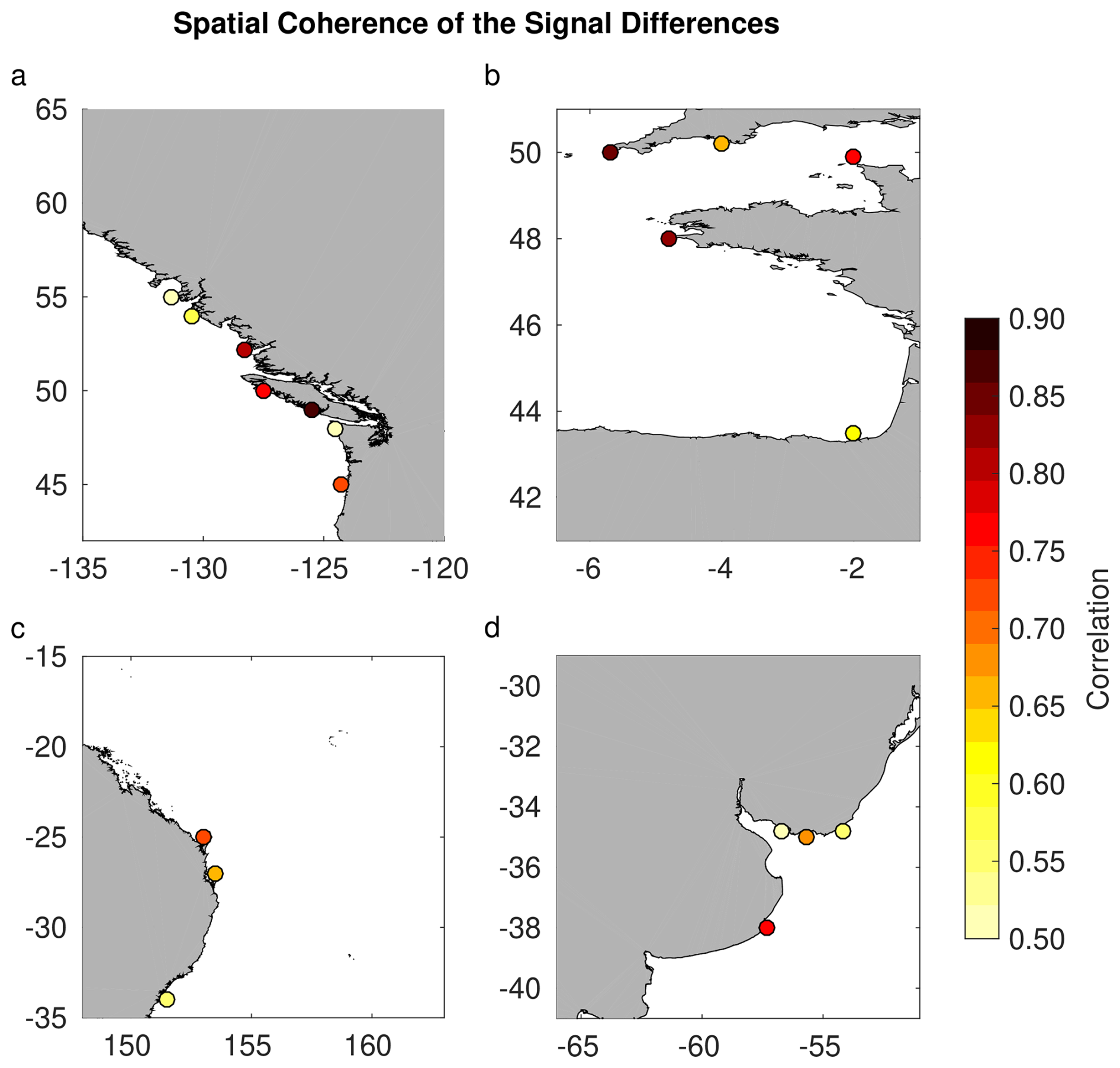
Figure 7 The spatial coherence of the Signal Differences in the west coast of North America (a); the Bay of Biscay (b); northeast Australia (c) and the Río de la Plata basin Argentina/Uruguay (d). The correlations are significant at the 95 % Confidence Interval (CI).

We examine the nature of the Signal Differences further by correlating, at each tide gauge: (1) the time series from tide gauges and altimetry (Fig. 8a); (2) the Signal Differences with the tide gauge time series (Fig. 8b); and (3) the Signal Differences with the altimetry time series (Fig. 8c). From a total of 229 tide gauges, 204 bins had a significant correlation (at the 95 % CI) between tide gauge and CMEMS altimetry, with an average correlation of 0.82 (Fig. 8a). In general, high correlations between tide gauges and altimetry show low SDs of Signal Differences, especially in the central and western Pacific Ocean. This indicates that, in general, the Signal Differences are due to signals that are observed by one of the instruments (either the tide gauge or altimetry) but not the other. Note, however, that a high correlation does not always mean that there is a low Signal Differences as there may be a scale factor between the altimetry and the tide gauge time series. There are a few locations (including the south-east and west coasts of South America and the southern west coast and northeast coast of Great Britain) that show correlation values between 0.4 to 0.6. These lower correlation values coincide with higher SD values of the Signal Differences.

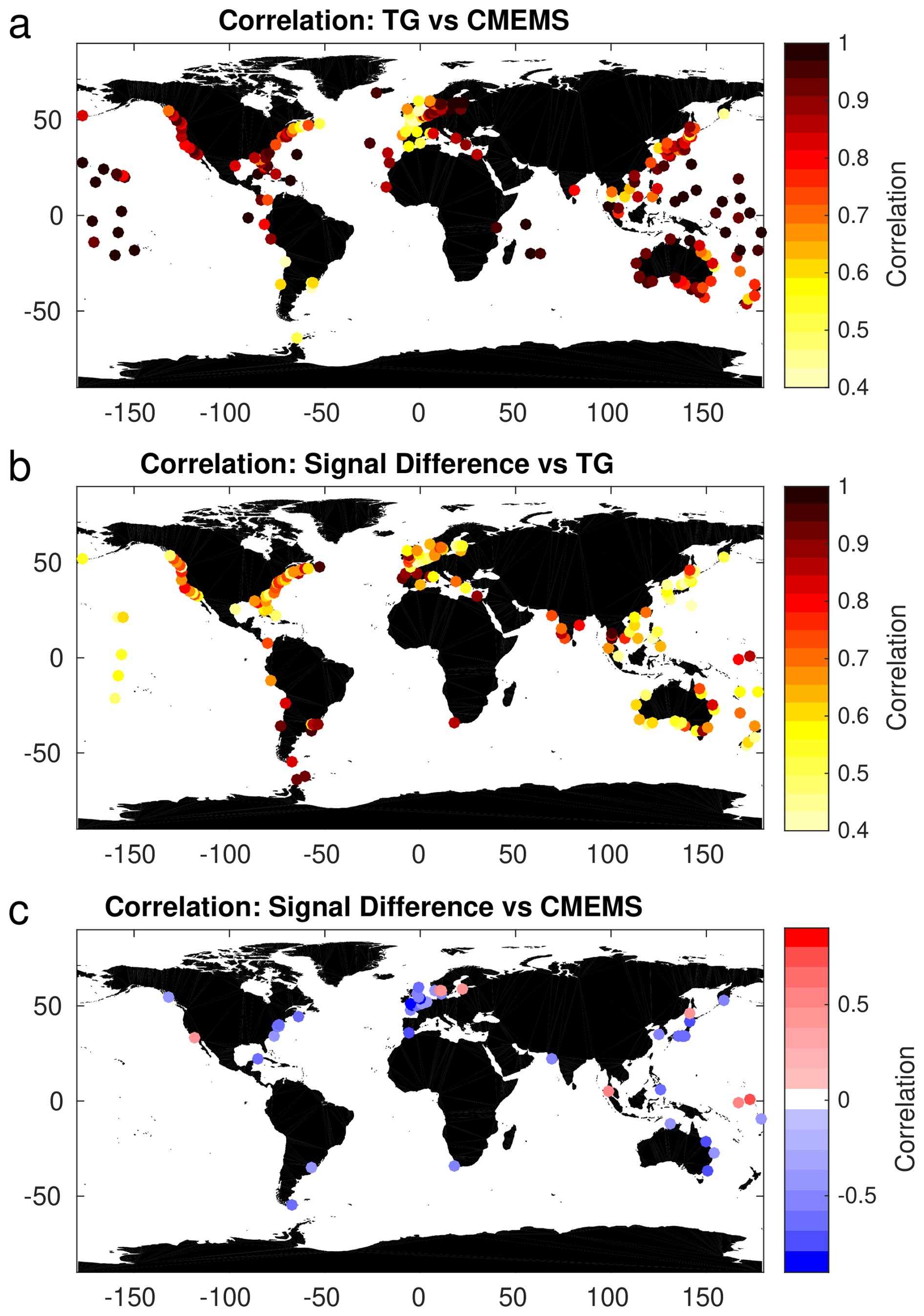
Figure 8 Correlations between tide gauge and CMEMS altimetry (a); between the Signal Differences and tide gauges (b); and between Signal Differences and CMEMS altimetry (c). Only correlations that are statistically significant at the 95 % CI are shown.

A total of 146 (out of 229) locations had a statistically significant correlation between tide gauge observations and their corresponding Signal Differences (Fig. 8b), whereas only 45 locations had significant correlations between altimetry and Signal Difference (Fig. 8c). If we break this down further, 119 locations had significant correlations of Signal Differences with tide gauge observations only; 18 locations had a significant correlation with altimetry only; and finally, 27 locations had a significant correlation with both the tide gauge and altimetry observations. In summary, a total of 164 locations out of 229 had a significant correlation with the Signal Differences (i.e. 119_TG+18${}_{\mathrm{CMEMS}}+{\mathrm{27}}_{\mathrm{TG}\mathrm{and}\mathrm{CMEMS}}=\mathrm{164}$).

The fact that Signal Differences at most locations are correlated with tide gauges but not with altimetry tells us something important: that signals detected by the tide gauges but not observed by altimetry are contributing to the Signal Differences (Fig. 8b and c). It is not surprising that the significant correlations between Signal Differences and altimetry observations displayed in Fig. 8c are mostly negative because the Signal Differences are defined as tide gauge minus altimetry. The central and western Pacific Ocean and western Indian Ocean show low SD of the Signal Differences (Fig. 6) with high correlation between the tide gauge and altimetry (Fig. 8a), yet few significant correlations between the Signal Differences and either tide gauge or altimetry (Fig. 8b and c). This tells us that both sensors are seeing the same sea level signal in these regions. Moreover, if a large SD Signal Differences are observed at tide gauge where the correlation between altimetry and tide gauges is very high, then this should be largely due to a scale factor between the altimetry and tide gauge time series. In this case, the Signal Differences should be highly correlated to both the tide gauges and the altimetry. This is observed in 16 out of the 27_{TG  and  CMEMS} grouped locations (half of which are in the north/northwest of Europe) that had a significant correlation between tide gauge and altimetry with a corresponding mean SD of the Signal Differences of 2.1 cm.

The southern west coast of South America is intriguing. Here, there are high SDs of Signal Differences (Fig. 6), with significant correlations between tide gauge and altimetry, (i.e., 0.4 to 0.6) but no significant correlations between Signal Differences and altimetry. This implies that the tide gauge observations are detecting something that the altimeter does not, even though the correlations between tide gauge and altimetry are significant.

Western Australia and west coast of Central America are similar to the west coast of South America except that the correlations between the tide gauges and altimetry in Western Australia and west coast of Central America are very strong compared with South America. This high correlation can occur even if the SDs of the Signal Differences are high, such as when both tide gauge and altimetry observations are picking up the same sea level signal but with different amplitudes, leading to higher Signal Differences.

3.2 Relationship of the Signal Differences with Wind and the ENSO

So far, we have shown that the Signal Differences are not due to random instrumental errors, and thus it may be explained through external factors (components) such as atmospheric forcing on sea level. For many decades researchers have investigated wind as a contributing factor, influencing sea level changes along the coasts (e.g. Calafat et al., 2018; Gill and Clarke, 1974; Piecuch et al., 2016; Johansson et al., 2022; Sturges and Douglas, 2011 and The Climate Change Initiative Coastal Sea Level Team, 2020). Here we correlate the Signal Differences with the zonal and meridional components of the, u and v (Fig. 9a and b, respectively). Globally, there are strong coherent spatial patterns of correlations (both positive and negative) between the Signal Differences and wind (u, v), with absolute correlation values of 0.5 or more at many locations. The Pacific coast of the US, Australia, the UK and Japan are regions that show particularly coherent structures, whereas in the west and central Pacific Ocean the wind appears to be less of a factor to explain the Signal Differences.

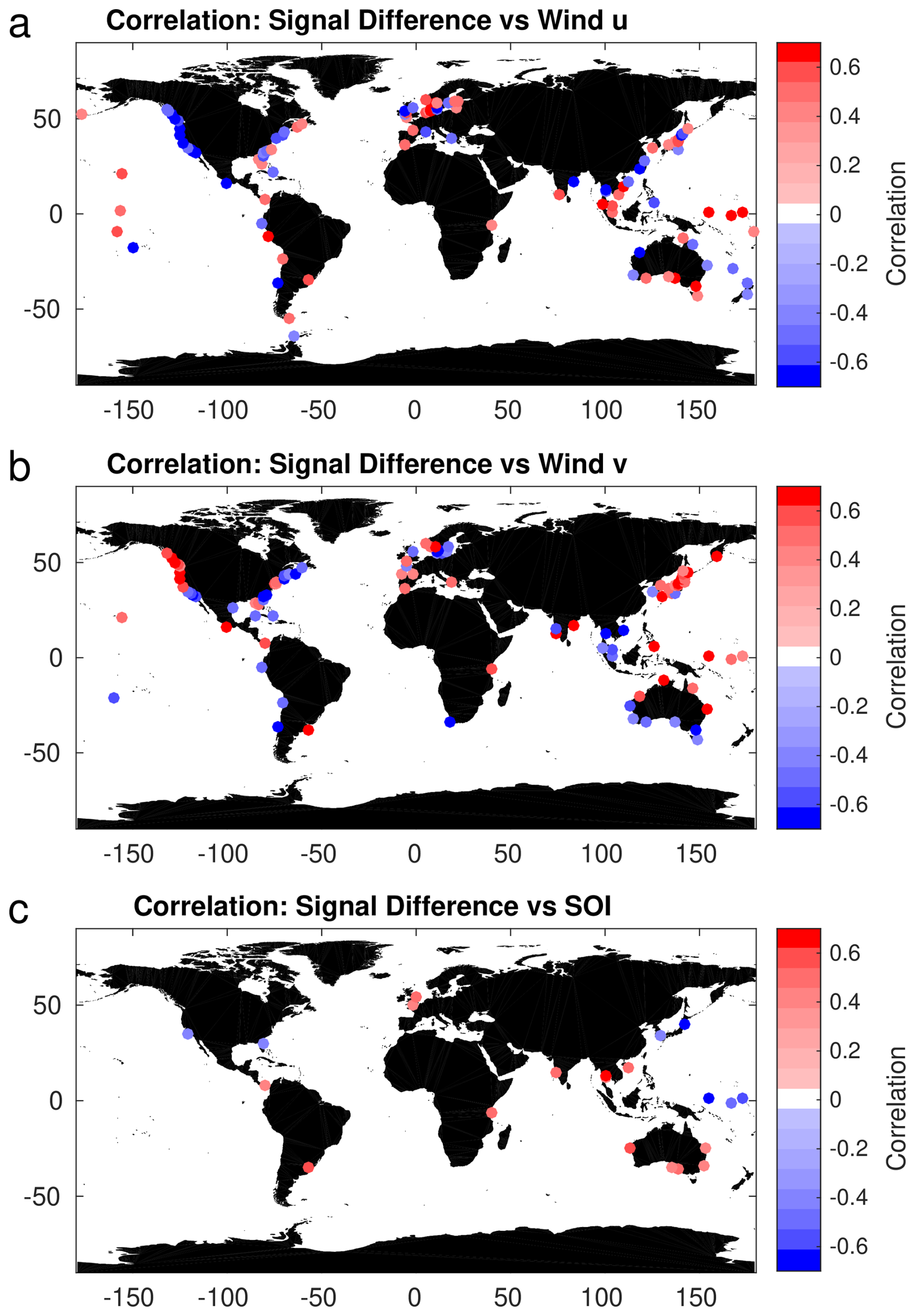
Figure 9 Correlations between the Signal Differences and wind u parameter (a); between the Signal Differences and wind v (b); and between the Signal Differences and the Southern Oscillation Index (SOI) (c). Only correlations that are statistically significant at the 95 % CI are shown.

Another factor that could explain the Signal Differences is sea-level variability associated with the ENSO, particularly in the Pacific Ocean, as this has been shown to play an important role in the interannual climate variability (Han et al., 2017  Hamlington et al., 2020a; McPhaden et al., 2006; Nerem et al., 2010; Royston et al., 2018; Zhang and Church, 2012). Calafat et al. (2014) also showed that the ENSO influence on GMSL is not well captured by EOF reconstructions that use the EOF0. Here, we correlate the annual SOI climate index with the Signal Differences and found significant correlations at many tide gauge locations, implying that the Signal Differences has an SOI component (Fig. 9c). In most cases, the significant correlations were positive along many coastlines, with the exceptions of a few coherent clusters of negative correlations to the northeast of Papua New Guinea, Japan and southern USA. To some extent, the correlations with the SOI index might reflect the effects of local wind forcing on sea level, but they could also indicate a contribution from remote atmospheric forcing associated with the ENSO.

3.3 Multiple Linear Regression for the Signal Differences (1994–2020)

The significant correlations that we have found of wind and SOI parameters against the Signal Differences in many regions provide the basis to create a multiple linear regression model that includes these variables. Here, we investigate three multiple linear regression models (Models 1 to 3, Eqs. 3 to 5)

To assess the performance of the three regression models, we begin by focusing on the same four regions (Fig. 7) that showed strong regional coherence of the Signal Differences (i.e., west coast of North America, the Bay of Biscay/English Channel, Northeast Australia, and South America). We correlate the prediction of the regression model with the Signal Differences, both averaged over the corresponding region. Fig. 10 shows that the wind plays an important role in explaining a large part of the Signal Differences in all four regions, with correlations between the Signal Differences and Model 1 ranging from 0.52 to 0.75. Progressively adding the SOI and the tide gauge parameter (Models 2 and 3) generally improves the correlation and scale factor, although to a lesser extent and with regional variation in correlations. Please note that the regression Model 2 (blue line in Fig. 10c) appears to be missing because the regression Model 3 (red line) has superimposed itself on the regression Model 2. This is reflected as the correlation between spatially averaged Signal Differences and regression Models 2 and 3 have the same correlation of 0.78.

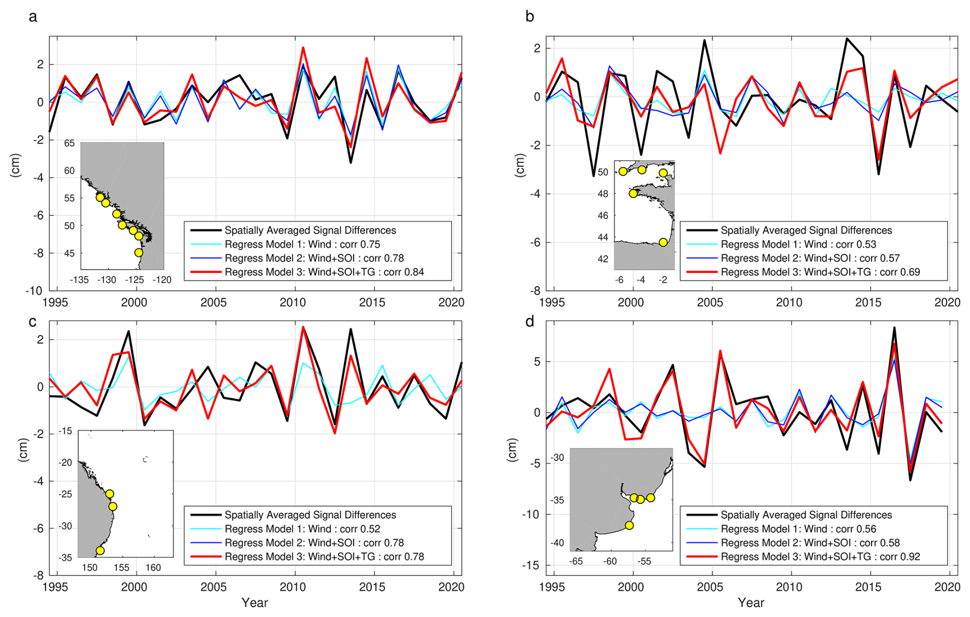
Figure 10 Time series of spatially averaged Signal Differences from the tide gauge within each region (insert) compared with the time series from the three regression models, for the west coast of North America (Washington State and British Columbia (a); Bay of Biscay/English Channel (b); northeast Australia (c) and the Río de la Plata basin Argentina/Uruguay (d). These regions are the same as Fig. 7.

We have also assessed the performance of Model 1 and Model 3 at each of the 285 tide gauges by computing the correlation and the explained variance (Fig. 11). Model 1 (only wind) shows a globally averaged correlation with the Signal Differences of 0.48 and an average explained variance of 26 %. The highest correlation values are found along the west coasts of North America, India and Australia (Fig. 11a and b). Model 3 (wind, SOI and TG as predictors) show significantly higher correlations and explained variance, with globally averaged values of 0.67 % and 49 % (Fig. 11c and d), respectively.

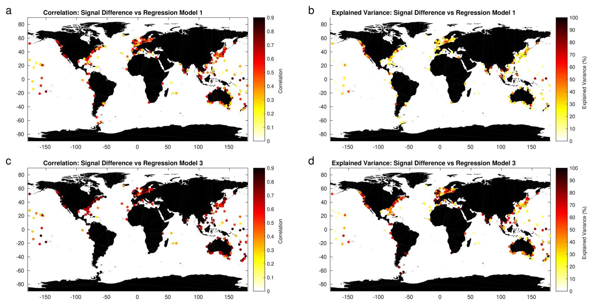
Figure 11 The correlations (a) between the Signal Differences and the regression Model 1, Eq. (3) and the corresponding explained variance (b). The correlations (c) between the Signal Differences and the regression Model 3, Eq. (5) and the corresponding explained variance (d).

3.4 Adjusting the Tide Gauge Observations prior to GMSL Reconstruction using the Signal Differences Multiple Linear Regression Model

Here, we use regression Model 3 to correct for the Signal Differences at each tide gauge from 1941 to 2020 prior to computing the EOF reconstruction, as Model 3 had the best overall correlation (Figs. 10 and 11) and their corresponding variance explained (Fig. 11). To do this, we first derive the Model 3 parameters using the period from 1994 to 2020 where both the wind (u, v) and the tide gauge predictors were detrended prior to computing the EOF reconstruction and then the Signal Differences were determined at each tide gauge and were also extrapolated back in time (1941 to 1993). The corrected EOF reconstruction compared with our uncorrected reconstruction as well as the “true” GMSL (1993 to 2020) from the altimetry period are shown in Fig. 12. The trends for both the uncorrected and corrected EOF reconstruction are statistically the same, 1.9 ± 0.7 mm yr⁻¹, 2.0 ± 0.7 mm yr⁻¹, respectively. For the altimetry period (1993 to 2020) the trends show that uncorrected EOF reconstruction (3.3 ± 0.6 mm yr⁻¹); corrected reconstruction (3.5 ± 0.5 mm yr⁻¹) and the “true” GMSL trend (3.2 ± 0.5 mm yr⁻¹) are also statistically the same. This means that the trends are not influenced by the Signal Differences correction.

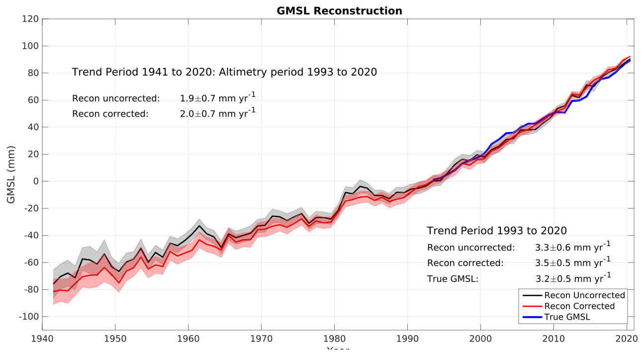
Figure 12 Comparison of uncorrected EOF reconstruction (black line) derived from Eq. (2) and the corrected EOF reconstruction (red line). The 1-sigma uncertainty intervals, shaded grey and light red respectively, reflect the sensitivity of the reconstruction to the number of tide gauges as evaluated SD using a bootstrap method. The “true” GMSL derived from altimetry is shown as a blue line (1994 to 2020).

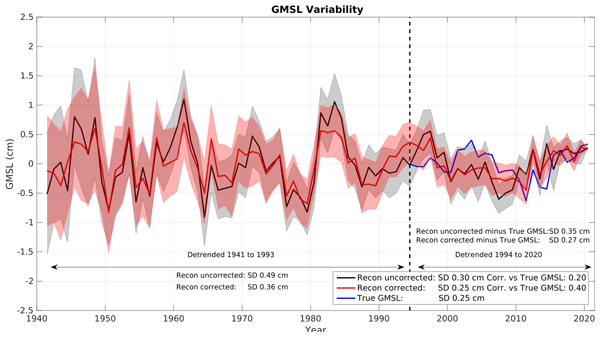
Focusing now on the reconstructed variability (Fig. 13), both the uncorrected and corrected reconstruction of GMSL show in general a reduction in the later period (1994–2020) compared with the earlier period (1941–1993). We find that for the earlier period, the corrected EOF reconstruction displays reduced variability compared with the uncorrected reconstruction, with SDs of 0.36 and 0.49 cm, respectively. For the later period, we can also include the “True” GMSL from altimetry in the comparison. The corrected GMSL reconstruction shows a significantly higher correlation with the true GMSL with a value of 0.40, compared with 0.20 for the uncorrected reconstruction. The magnitude of the GMSL variability is also better captured by the corrected reconstruction, as quantified by the SD of the time series, which is 0.25 and 0.30 cm for the corrected and uncorrected reconstructions, respectively, compared to a SD of 0.25 cm for the true GMSL. The difference between our uncorrected reconstruction and the true GMSL shows a SD of 0.35 cm, whereas the difference between the corrected reconstruction and the true GMSL gives a SD of 0.27 cm. This implies a reduction of 23 % in the error associated with the reconstruction of the GMSL variability.

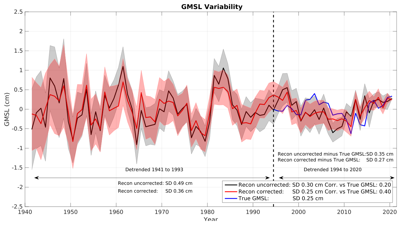
Figure 13 The variability of the GMSL that has been detrended for two time periods 1941 to 1993 and 1994 to 2020 showing the uncorrected EOF reconstruction (black line) derived from Eq. (2) and the corrected EOF reconstruction (red line). The 1-sigma uncertainty intervals shaded grey (uncorrected) and light red (corrected) reflect the sensitivity of the reconstruction to the number of tide gauges as evaluated standard deviation (SD) using a bootstrap method. The detrended “true” GMSL derived from altimetry is shown as a blue line (1994 to 2020).

The earlier period in Fig. 13 had a larger uncertainty for both reconstructions (shaded regions) compared with the later period, most likely due to the smaller number of tide gauges compared with the later time period. The uncertainties of the uncorrected and corrected EOF reconstruction for the earlier period were similar except for the very strong 1983–1984 El Niño event where the corrected uncertainty was reduced. The later period generally shows a reduction of corrected uncertainty compared with uncorrected uncertainty, especially during the very strong El Niño events of 1997–1998 and 2015–2016. In addition, the later period shows that the corrected reconstruction (red line) lies closer to the true altimetry GMSL (blue line) for both of these very strong El Niño events. This does imply that uncorrected GMSL reconstruction did not capture ENSO events well.

4 Discussion and Conclusion

This study has shown that the use of EOF reconstruction to estimate GMSL variability is improved by adjusting the tide gauge observations for the Signal Differences prior to the EOF reconstruction. We found initially that the Signal Differences between the tide gauge observations and the altimetry data show regional spatial coherence along the coasts (e.g. Figs. 6 and 7). Furthermore, such differences are significantly correlated with tide gauges at most locations, but often not with altimetry (Fig. 8), which rules out observation errors as the cause of the differences. This suggests instead that the differences are due to real oceanographic signals that are not adequately captured by altimetry. The significant correlations (at 95 % CI) between the Signal Differences with wind and SOI globally (Fig. 9) enabled us to build Signal Differences multiple linear regression models at each tide gauge. Here, the Wind and SOI variables were used as predictors as part of the linear regression models to predict these Signal Differences before 1993, which are then applied to the tide gauge observations prior to the GMSL reconstruction, generating a corrected GMSL reconstruction. Model 3, Eq. (5) was found to be the most appropriate both regionally (Fig. 10) and globally (Fig. 11). A large fraction of the Signal Differences has been explained by wind forcing and/or the tide gauge data themselves through multiple linear regression. Although the SOI played a minor role in the regression model, it did play an important role in the northeast Australian region (Figs. 9c and 10c) as this area is influenced by the ENSO and is consistent with White et al. (2014).

The corrected GMSL reconstruction shows improved GMSL variability (Fig. 13), with a correlation of 0.40 compared with 0.20 for the uncorrected reconstruction. The corrected GMSL reconstruction also shows reduced variability than the uncorrected reconstruction, thus showing a better agreement with the true GMSL from altimetry. The GMSL variability was greater during the earlier period for both the uncorrected and corrected reconstruction although there was a reduced SD for the latter. The large uncertainty from the uncorrected GMSL reconstruction in Fig. 13 (shaded grey) corresponds with El Niño events (including the very strong events in 1982–1983, and 2015–2016) compared with the corrected GMSL reconstruction (shaded red), providing evidence that the uncorrected GMSL reconstruction did not capture ENSO well.

In some regions both the tide gauge and altimetry observations are detecting the same sea level signal. A lot of island tide gauge locations in the central Pacific Ocean straddle the Doldrums (5° S to 5° N), which has little wind. Beyond the latitudes of the Doldrums, the trade winds are a dominant feature and Yang et al. (2022) showed an acceleration in trade winds in the mid to late 1990s. It is not surprising that there is a strong correlation between tide gauge and altimetry because the sea level signal has a lack of wind or a stable large-scale trade wind component that the altimeter also detects. However, not all Pacific islands followed this trend, as a few locations had a significant correlation between Signal Differences with wind (Fig. 9) and had a low or medium magnitude of the Signal Differences. No significant correlation between Signal Differences and altimetry were shown at these island sites (Fig. 8c) implying that these locations have some sea level signal, such as the wind component, that the altimetry did not capture or other physical mechanisms contributing to the difference in sea level variability in the region (e.g. The Climate Change Initiative Coastal Sea Level Team, 2020). Thus, more understanding of the atmospheric and oceanographic processes can lead to other factors that may influence the Signal Differences, providing an improved regression model.

A large fraction of the Signal Difference between tide gauge and altimetry observations is likely explained by wind-driven coastal trapped waves, which can communicate sea-level signals over long distances along continental shelves around the world (Woodworth et al., 2019; Hughes et al., 2019). These waves are an important driver of coastal sea-level variability, for example in Europe (e.g., Calafat et al., 2012; Calafat et al., 2013), Australia (e.g. Maiwa et al., 2010; White et al., 2014; Woodham et al., 2013) and the United States of America (Battisti et al., 1984; Connolly et al., 2014; Gutiérrez et al., 2014; Merrifield, 1992). Coastal trapped waves have relatively small cross-shelf scales (comparable to the shelf width), and thus, while they can produce coherent sea-level variability along long stretches of coastline, their effects are confined to the coastal zone. As a result, such boundary-wave signals may not be fully captured by altimetry, contributing to differences with tide gauge observations. Our correction for the Signal Difference may partially account for these effects through wind and ENSO-based covariates, since both are known factors for coastal trapped waves, but not fully because coastal trapped waves are often remotely forced, whereas our wind covariates are purely local.

We also note that the corrected and uncorrected GMSL reconstructions display slightly different trends (Fig. 12), which are not statistically significant but are visually noticeable. A plausible explanation is that modifying the variability at individual tide gauges through our correction alters their relative weights (see Eq. 2) in the GMSL reconstruction, which will necessarily influence not only the reconstructed GMSL variability but also its trend.

Further advancements to the Signal Differences regression model beyond this study will be to investigate the locations where the magnitude of Signal Differences is low and determine if these locations are necessary for a Signal Differences regression model to be applied. As previously mentioned, this study assumed that the regression coefficients are constant with time (1994 to 2020), but this temporal stability becomes important for a Signal Differences model to be applied to tide gauge data prior to 1993. Temporal sensitivity testing during the altimetry period provides a good starting point for future altimetry development by targeting these regions where the Signal Differences are seen by the tide gauge observations but not by the altimeter. In addition, further work can investigate other coastal processes that contribute to the Signal Differences beyond the local wind and SOI climate index found here, such as the effects of river discharge in local and regional sea level variability (Piecuch et al., 2018). Piecuch (2023) pointed out that there may be implications for twentieth-century GMSL reconstructions as the river effects on tide gauges such as in the Río de la Plata should be removed prior to GMSL reconstruction. Furthermore, determining the wind angle of approach to the coastline may be a useful enhancement to the regression model.

Another limitation potentially contributing to the differences between altimetry and tide gauge observations is VLM, which is only captured by tide gauges. VLM is often assumed to be well represented by a linear trend, in which case it would have limited influence on the reconstruction weights and resulting GMSL. However, recent studies have shown that this assumption does not always hold, with both non-linear trends and higher-frequency variability present at some locations (Oelsmann et al., 2024; Wang et al., 2025). While non-linear trends are expected to have only a minor effect on the reconstruction weights, shorter-term variability may have a larger influence, and accounting for it could improve GMSL reconstruction by reducing the signal difference. To test this and following Wang et al. (2024), we recalculated the GMSL reconstruction after correcting the tide gauge records for contemporary GRD-induced VLM, using GRD data from Frederikse et al. (2020). Unfortunately, we found that applying the GRD correction did not improve the GMSL variability of the corrected reconstruction. An alternative would be to use GPS observations of VLM, however, long, continuous GPS records are available at only a very limited number of tide gauge sites.

In conclusion, the differences between tide gauges and altimetry (Signal Differences) are significantly correlated along the coast, and these differences are correlated well with local winds, and it appears that this is not always adequately captured by altimetry. The over estimation in variability of the GMSL EOF reconstruction has been shown to be reduced by applying a Signal Differences correction model to the tide gauge observations prior to reconstruction. Correcting the Signal Differences as a first step through the regression model (Model 3) prior to the reconstruction reduces the SD of the reconstructed GMSL variability by 23 % and significantly increases the correlation with observed altimetry GMSL (1994–2020). The Signal Differences were extrapolated prior to 1993 which showed the corrected EOF GMSL reconstruction variability also had reduced uncertainty compared with the uncorrected reconstruction. Caution is needed as the Signal Differences at a tide gauge may not be due to a physical oceanographic signal but instead just bad altimetry data, tide gauge data or both.