The vertical structure of mesoscale eddies in the Azores Current corridor: a combined altimetry-Argo analysis

Temperature and salinity, derived from over 10 000 Argo profiles, are combined with 20 years of eddy trajectories and absolute dynamic topography maps to characterise the vertical structure of mesoscale eddies within the Azores Current corridor (AzCCo) from the surface to 1500 dbar. From east to west, our statistics reveal an intensification of anomaly maxima (from ∼ 0.5 °C and 0.1 to above ∼ 1.5 °C and 0.2 in salinity) and a deepening of their core location in the water column (from ∼ 250 to ∼ 750 dbar) for both anticyclones and cyclones. Anticyclones are characterised by a relatively depth-uniform structure, exhibiting warm, salty cores, while cyclones are more vertically structured, with a well-defined subsurface maximum featuring cold, fresh cores along the AzCCo. These zonal differences are associated with the origins of the sampled eddies and their dynamical properties on either side of the Mid-Atlantic Ridge (MAR). In the western region, eddies are more strongly influenced by remotely generated structures associated with Gulf Stream branches, contributing to higher anomaly amplitudes. To investigate the mechanisms responsible for these anomalies, an isopycnal decomposition of temperature and salinity anomalies is applied, separating them into two components: heave (HEV), associated with vertical deflections of isopycnal surfaces, and spice (SPI), representing variations along isopycnal surfaces. These components are linked to two main eddy transport mechanisms: eddy pumping and eddy trapping. HEV dominates the resulting vertical structures of temperature and salinity within the water column, indicating that most eddy-induced anomalies originate from eddy pumping, manifested as deflections of the isopycnal surfaces. This mechanism produces warmer, saltier anomalies within anticyclonic eddies due to downwelling of the isopycnal surfaces and colder, fresher anomalies within cyclonic eddies due to upwelling of the same surfaces. SPI exhibits higher values within the upper ∼ 250 dbar to the east of the MAR, reflecting the tendency of surface eddies to trap different water masses. Finally, absolute values of isopycnal vertical displacement above 50 dbar, from the surface to the 1500 dbar level, demonstrate the significant impact of these mesoscale structures throughout the water column. Overall, these results highlight the AzCCo as a vertically driven mesoscale regime in which eddies primarily redistribute thermohaline properties through isopycnal displacement rather than lateral transport.

1 Introduction

Mesoscale eddies play a fundamental role in redistributing heat, salt, and momentum in the ocean (e.g., Chelton et al., 2011; Treguier et al., 2012; Frenger et al., 2015). Part of this transport occurs through the advection of water masses with distinct thermohaline properties within coherent eddy cores (eddy trapping). However, a recent study by Abernathey and Haller (2018) has shown that this mechanism accounts for only a limited fraction of the total transport, with a significant contribution arising from stirring and filamentation surrounding the eddies. In addition, vertical motions induced by mesoscale structures (eddy pumping) influence the nutrient transport, while their rotation modulates the horizontal distribution of biogeochemical tracers (e.g., Martin and Richards, 2001; Gaube et al., 2014; Mahadevan, 2016; Keppler et al., 2024).

The Azores current (AzC) is a highly turbulent zonal jet located around 34° N, east of the Mid-Atlantic ridge (MAR), characterised by high eddy kinetic energy (EKE) values exceeding 200 cm² s⁻² (Fig. 1), the highest in the eastern subtropical North Atlantic. The current system and its associated frontal zone have been revisited several times over the last decades (e.g., Gould, 1985; Juliano and Alves, 2007; Frazão et al., 2022). The latitudinal band surrounding the jet, hereafter referred to as the Azores Current Corridor (AzCCo), is characterised by a combination of coherent eddies, meanders, and filaments, mostly generated by baroclinic instability of the jet as well as by remote eddy propagation into the region (Klein and Siedler, 1989; Alves and De Verdière, 1999). Different zonal sectors with distinct mesoscale activity have been identified within the AzCCo, with a general decrease in EKE values from west to east. These patterns are strongly influenced by topography, particularly the MAR, which acts as a partial barrier between the eastern and western basins. West of the MAR, eddies are not only more energetic but also exhibit larger amplitudes, greater radii, and stronger swirl velocities (see Silva-Fernandes and Peliz, 2020, their Fig. 7b, c and d). East of the MAR, Barbosa Aguiar et al. (2011) identify three sub-regions: western sector between the MAR and the Seewarte Seamount Chain (SWSM) (∼ 28° W); central sector between 28 and 20° W; and eastern sector extending toward the Gulf of Cádiz.

While the surface expression and statistical properties of eddies in this region are relatively well documented (e.g. Barbosa Aguiar et al., 2011; Silva‐Fernandes and Peliz, 2020), a systematic study of their internal structure and impact on the water column is still missing. Existing studies comprise mainly isolated events derived from in situ data (e.g., Pingree et al., 1996; Pingree and Sinha, 1998; Mouriño et al., 2002; Mouriño et al., 2003), with most of these studies focusing on the large cyclonic eddies along the “Storm Corridor” (∼ 34° N; Pingree, 2002). These large cold-core cyclones are characterised by horizontal temperature anomalies of ∼ 2.5 °C between 200 and 600 dbar. Pingree et al. (1996) also reported isopycnal displacements of ∼ 200 dbar, extending from the surface to near the seafloor (∼ 4000 m).

More recently, Pegliasco et al. (2015) characterised the vertical structure of two clusters of eddies using Argo floats originating from the Canary upwelling system, partially overlapping the southern flank of the AzCCo (west of 20° W). A shallow cluster (cores at ∼ 0–200 m), dominated by anticyclones, exhibits weak positive anomalies and short propagation pathways, forming part of the Canary Corridor (CnCo). In contrast, a deeper cluster (maxima between 200 and 600 m), dominated by cyclones, shows negative temperature and salinity anomalies ($\sim -$0.5 °C and −0.07) and extends to depths of 600–800 m. This latter group propagates as far as 40° W, near the MAR, and is associated with the Madeira Corridor (MdCo; Sangrà et al., 2009). Similarly, Amores et al. (2017) used composites of Argo floats and altimetry (Sea Level Anomaly – SLA), covering part of the AzC southern flank (∼ 32° N). They reported peak anomalies at ∼ 150 m for anticyclones and 400–800 m for cyclones, with potential temperature anomalies exceeding 1 °C and salinity anomalies of ∼ 0.2, the latter being slightly stronger in cyclones. Anticyclonic (cyclonic) eddies are generally characterised by warm and salty (cold and fresher) cores, with signals extending down to ∼ 1200 m. West of the ridge, based on the analysis of SOFAR float trajectories launched on both sides of the MAR, Ollitrault and Colin de Verdière (2002) reported that eddies in this region exhibit a southward flow south of 38° N and generally migrate along the western flank of the ridge. Furthermore, their analysis showed that cyclones (anticyclones) are characterised by cold (warm) cores at approximately 770 dbar.

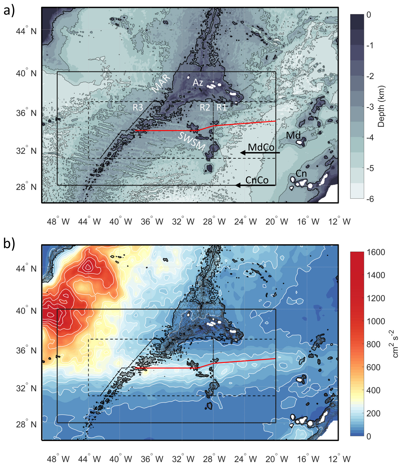
Figure 1 (a) Bathymetric map. MAR – Mid-Atlantic Ridge; SWSM – Seewarte Seamount Chain; MdCo – Madeira Corridor; CnCo – Canary Corridor; Md – Madeira Island; Cn – Canary Island; Az – Azores Islands. Bathymetric contours are drawn every 500 m from the surface down to 6 km depth. The thick black contour represents the 2500 m bathymetry, and the thin black ones the 4000 and 5000 m bathymetry. (b) Spatial distribution of mean EKE (cm² s⁻²) for the period 2005–2017. Contours are highlighted in white every 50 up to 400 cm² s⁻², and then every 200 cm² s⁻² thereafter. Bathymetric contours are drawn every 500 m from the surface down to 2500 m depth. The thick black contour represents the 2500 m bathymetric contour. In both panels, the black box indicates the study area, and the three dashed boxes represent the regions directly associated with the Azores Current Corridor: the eastern region (R1), the central region (R2), and the western region (R3). The red line represents the mean axis location of the AzC, following Silva-Fernandes and Peliz (2020). Land is shown in white.

In addition to locally generated eddies, Mediterranean water eddies (meddies) are also present in the region, particularly east of the MAR (east of the SWSM and the Azores Plateau (AzP)) (Bashmachnikov et al., 2015). These structures transport Mediterranean water (MW) with strong thermohaline contrasts relative to the surrounding ocean, generating pronounced temperature and salinity anomalies at intermediate depths (∼ 800–1200 dbar), with values exceeding 0.5 °C and 0.2 in salinity over vertical scales of several hundred meters (Richardson et al., 1991; Bashmachnikov et al., 2015). Meddies are predominantly anticyclonic, although cyclonic meddies have also been reported, exhibiting positive temperature and salinity anomalies and vertical extensions from approximately 500 to 1300 dbar (Richardson et al., 2000; Barbosa Aguiar et al., 2013). In contrast to locally generated eddies, meddies are expected to exhibit higher thermohaline anomaly values, offering a useful contrast with respect to different mechanisms of eddy-induced anomalies.

Collectively, previous studies have provided a detailed description of the surface eddy field and documented a number of isolated subsurface structures, but they lack a unified three-dimensional characterisation of eddies across the AzCCo. In this work, we address these gaps by analysing more than 10 000 Argo profiles combined with 20 years of altimetric data and an eddy atlas (AVISO+, Sect. 2.3). We characterise the vertical structure of composite mesoscale eddies in the AzC corridor (AzCCo) and explore the concepts of Spice (SPI) and Heave (HEV), relating the observed variations in climatological temperature and salinity fields to eddy trapping, associated with the advection of distinct water masses, and eddy pumping, manifested as the deflection of isopycnal surfaces driven by the internal structure of anticyclonic and cyclonic eddies.

The main research questions addressed in this study are as follows:

1. What is the typical vertical structure of eddies in the Azores Current corridor?

2. Which mechanisms – reflected by HEV and SPI anomaly signatures – dominate the generation of internal temperature and salinity anomalies within eddies?

3. How does the presence of mesoscale turbulent structures affect the water column in our study region?

Details of data and analysis methods are described in Sect. 2, and the results obtained are presented in Sect. 3. A brief discussion of the principal aspects of this work is outlined in Sect. 4, and answers to our initial questions are drawn in Sect. 5.

2 Data and methods

2.1 Argo floats

We used 20 997 Argo individual profiles (Argo, 2026; https://usgodae.org/cgi-bin/argo_select.html, last access: 7 August 2026) inside our study region between 2000 and 2020. These profiles were later pre-processed considering the following criteria: (1) The profiles' data (temperature, salinity, and pressure) were filtered, retaining those with a GOOD quality flag (equal to 1 or 2 according to https://archimer.ifremer.fr/doc/00187/29825/, last access: 7 August 2026). Adjusted values were used when available; (2) Profiles with their first value below 20 dbar and the last above 1500 dbar were discarded; (3) each profile should have at least 30 vertical measurements, with a depth difference between two consecutive measurements that should be smaller than 25 dbar from the surface to the 100 dbar level, 50 dbar from the 100 to 300 dbar layer, and smaller than 100 dbar below 300 dbar (these intervals were also used in Chaigneau et al., 2011). In the end, 10 034 profiles were retained, corresponding to 48 % of the initial number.

The Gibbs SeaWater oceanographic toolbox (GSW-OT; https://www.TEOS-10.org, last access: 7 August 2026) was used to compute conservative temperature (CT), absolute salinity (SA), density anomaly (RHO), and mixed layer depth (MLD), defined following de Boyer Montégut et al. (2004) as the depth at which potential density increases by 0.03 kg m⁻³ relative to the surface. All variables were interpolated to 10 dbar levels, and anomalies were computed relative to the World Ocean Atlas 2018 climatology (Boyer et al., 2018; WOA2018; https://www.ncei.noaa.gov/archive/accession/NCEI-WOA18, last access: 7 August 2026), for the Argo period (2005–2017). The climatological fields were interpolated in space and time to each Argo profile location and standard depth levels. In time, the interpolation consisted of selecting the climatological profile corresponding to the appropriate day of year, using a 12-month spline interpolation. The choice of the Argo period climatology ensures consistency between the climatological reference and the Argo-era sampling period, thereby avoiding differences arising from the inclusion of earlier, sparsely sampled periods in the climatology.

2.2 Vertical isopycnal decomposition 

The vertical isopycnal decomposition (hereinafter ISOD) has been applied not only to investigate the warming and/or freshening of specific water masses (e.g., Desbruyères et al., 2022) and ocean heat content variability (Zhang and Yan, 2017), but also to examine the vertical structure of mesoscale eddies and the mechanisms responsible for their internal physical and biogeochemical parameters' anomalies (e.g. Frenger et al., 2015; Gaube et al., 2014; Keppler et al., 2024). ISOD separates the contributions of two distinct processes to the generation of CT and SA anomalies: eddy trapping, associated with advection along isopycnal surfaces and quantified by SPI, and eddy pumping, associated with the vertical displacement of isopycnal surfaces and quantified by HEV, which is positive (negative) for downward (upward) isopycnal displacements.

In this work, all anomalies are defined as differences between Argo profiles and the climatological fields projected onto neutral isopycnal surfaces. Following Bindoff and Mcdougall (1994) and later Han and Yan (2018), the ISOD equation can be written as:

$$\begin{array}{}\text{(1)}& \begin{array}{rl}\mathrm{\Delta }X{|}_{\mathrm{p}}& \cong X_{\mathrm{SPI}}+(-X_{\mathrm{HEV}})+\text{residual}\\ & \cong \mathrm{\Delta }X{|}_{\mathrm{n}}+(-\mathrm{\Delta }p{|}_{\mathrm{n}}\mathrm{\nabla }X)+\text{residual}\end{array}\end{array}$$

where ΔX|_p represents the total anomaly at a pressure level, ΔX|_n the anomaly along a neutral isopycnal surface (NIS), $-\mathrm{\Delta }p{|}_{\mathrm{n}}$ the vertical displacement of neutral surfaces and is expressed in pressure coordinates (dbar) and defined as the difference in pressure between Argo and climatological profiles for the same NIS, and ∇X is the vertical gradient of the climatological field. HEV and SPI are expressed in the same units as the corresponding variables (CT and SA anomalies). The residual (RES) term accounts for unresolved processes such as mixing and diffusion and is expected to be small in a well-stratified ocean.

The ISOD of CT and SA was computed as follows. NIS were calculated using TEOS-10 routines (http://www.teos-10.org/preteos10_software/neutral_density.html, last access: 7 August 2026, Jackett and Mcdougall, 1997) and interpolated onto a fixed grid. CT, SA, density, and pressure were then mapped onto each NIS. SPI and IVD were computed as differences between Argo and climatology along each NIS and subsequently interpolated back to pressure coordinates. The HEV component was calculated as $-\mathrm{\Delta }p{|}_{\mathrm{n}}\mathrm{\nabla }X$. Total anomalies (ΔX|_p) were obtained in pressure space as Argo minus climatology, and the residual was defined as the difference between the total anomaly and the sum of SPI and HEV.

In summary, each Argo profile was converted into profiles of CT and SA anomalies, as well as IVD, HEV, and SPI (for both CT and SA). These metrics were then used to construct the eddy composites, which are analysed to assess how mesoscale structures affect the water column in our study region.

2.3 Eddy tracking and Argo co-localisation

The mesoscale eddy trajectory atlas product version 3.2 (hereinafter META2022), produced by SSALTO/DUACS and distributed by AVISO+ (https://www.aviso.altimetry.fr/en/data/products/value-added-products/global-mesoscale-eddy-trajectory-product.html, last access: 7 August 2026), was used to identify and track eddies in absolute dynamic topography (ADT) maps using a geometric tracking method (Pegliasco et al., 2022) based on spatial proximity and contour overlap between successive time steps. Only eddies with a tracking lifetime longer than 10 d were considered in this study. Absolute dynamic topography (ADT) maps between 2000 and 2020 from the Copernicus Marine Service (CMEMS; https://data.marine.copernicus.eu/, last access: 7 August 2026) were used. The gridded product is based on merged observations from multiple satellite missions with $\mathrm{1}/\mathrm{4}$° spatial resolution and daily temporal resolution. Although the grid spacing is relatively high, the mapped fields are generated through interpolation of along-track measurements, with an effective spatial resolution of ∼ 200 km at mid-latitudes (Ballarotta et al., 2019; Taburet et al., 2019), resolving structures with a ∼ 50 km radius (Chelton et al., 2011, 2019). In our region, the first baroclinic deformation radius is approximately between the values of 30 and 50 km (Chelton et al., 1998), lying near the lower end of the mesoscale spectrum; features at this scale are therefore only partially resolved by the altimetric product, whereas eddies significantly larger are well captured. ADT fields were high-pass filtered using a first-order Bessel filter with a 700 km wavelength cutoff (Mason et al., 2014) to remove large-scale variability and then interpolated in space and time to the locations of the ARGO profiles. These maps were used as a background onto which the mesoscale eddy atlas trajectories were overlaid. In addition to the detected eddy trajectories, the META2022 contains information on their geometry, such as the speed contour (contour of maximum circum-average geostrophic speed for the detected eddy) or the effective contour (largest contour of the detected eddy) and kinematic properties such as amplitude (A – positive for both cyclones and anticyclones), radius (L) and swirl velocity (U). Additionally, each eddy's turbulent energy was computed ($\mathrm{EKE}=\frac{U^{\mathrm{2}}}{\mathrm{2}}$). One should note that the algorithm used to track the eddies allows the presence of virtual eddies up to a maximum of 4 d, where no speed contours are computed, and therefore these were not used in the Argo-localisation.

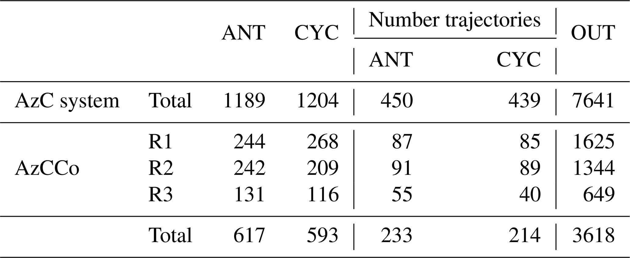
The co-localisation of the Argo floats inside META2022's eddies was conducted, creating a flag for each case where the Argo float emerged inside the speed contour (i.e., the contour of maximum circum-average geostrophic speed for the detected eddy) polygon that defined an anticyclone – ANT, or a cyclone – CYC. Those that were not inside any speed contour were considered outside an eddy – OUT. A total of 2393 Argo (24 %) emerged inside eddies and 7641 outside for the AzC system, while for the AzCCo region, a total of 25 % emerged inside eddies, from which 53 profiles are associated with meddies (see Table 1 for more details). The profiles associated with meddies were filtered according to Richardson et al. (1991) and Bashmachnikov et al. (2015) criteria: the CT and SA anomalies should be above 0.5 °C and SA anomalies above 0.2 of salinity for at least 200 dbar between 500 and 1500 dbar. These profiles were later separated from those used in the surface eddies' composites.

Table 1 Number of sampled eddies inside anticyclones (ANT), cyclones (CYC) and outside (OUT) and their number of associated trajectories in the AzC system and in the 3 regions of the AzC corridor.

2.4 Composite vertical structure 

Although different AzC regions along the current main axis have been identified in previous works (Barbosa Aguiar et al., 2011; Silva-Fernandes and Peliz, 2020), here we emphasise the division associated with the main topographic features and extend our analysis to the western flank of the MAR (Fig. 1a). Therefore, we will consider three regions: R1 between 20° W and the SWSM chain, R2 from 28° W to the western flank of the ridge following the 2500 m bathymetric, and R3 west of the ridge to 44° W (boxes in Fig. 1). To avoid ambiguities when eddies extend across regional boundaries, regional attribution was based on the location of the Argo float sampling the eddy rather than on the eddy centroid position.

After associating the eddies with different regions, a two-dimensional composite (considering the distance of each Argo to the eddy centre) and a vertical median profile (of all Argo profiles inside a region, independently of their position relative to the eddy's centre) of eddy anomalies (CT and SA) and IVD were computed. The latter was used not only to compare the two sign structures to the vertical median of Argo profiles emerging outside eddies along the AzCCo, but also to characterise the vertical structure of meddies as they are found in the eastern part of our domain.

The composites for each region were computed as follows: (1) a normalised distance for each Argo float to the eddy centre was calculated using the ratio ($d_{\mathrm{A}}/d_{\mathrm{I}}$); the distance of the Argo to the eddy centre (d_A) and the distance of the centre of the eddy centre to the nearest point of the speed contour (d_I) in the azimuth direction of the Argo float; i.e., along the line connecting the eddy centre and the Argo float position (see Fig. 2a for more details). Its x (east–west) and y (north–south) components were also computed, and the locations of the Argo profiles sampling the eddies in the regions along the AzCCo are shown in Fig. 2b. (2) An optimal interpolation (Barnes, 1973) with 3 iterations is conducted to interpolate each variable onto a regular 0.1 × 0.1 grid at each depth. (3) Further, to build the composites, we have assumed azimuthal symmetry (i.e., that eddies are circular structures and depend only on depth and distance from the centre). Although this is not verified for all eddies, in terms of statistics, a first decomposition into zonal and meridional mean sections revealed similar vertical structures (not shown).

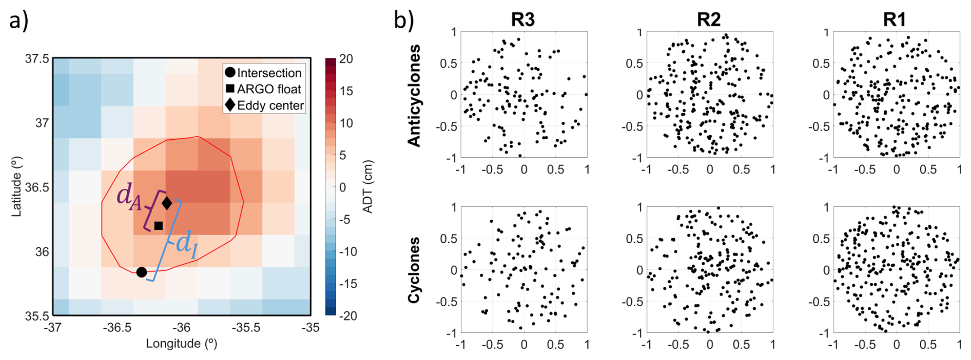
Figure 2 (a) Illustration of an anticyclone's characteristics: ADT (colours), eddy centre (black diamond), and the eddy speed contour (red line). The float's position (black square) and the intersection of a line (in the direction of the float azimuth) with the eddy speed contour (black circle) are also shown. The distances d_A and d_I were used to normalise the distance of every float to the eddy centre. (b) Normalised distance of the Argo profiles to the eddy centre for all points used to construct the eddy composite for the three AzCCo regions and both sign structures.

3 Results

3.1 Argo distribution and eddy field characterisation

The spatial distribution of Argo profiles emerging within anticyclonic (ANT) and cyclonic (CYC) eddies reveals a clear concentration east of the Seewarte Seamount Chain (SWSM), where the highest number of profiles is observed, particularly for cyclones (up to 24 profiles; Fig. 3a and c). In contrast, sampling is sparse south of 30° N, especially west of 28° W, where some grid cells contain no Argo observations. Profiles collected outside eddies (OUT) show a similar spatial pattern, with maximum densities located east of 28° W and in a secondary region centred near 31° N, 39° W (Fig. 3e). Figure 3b and d show the dynamic characteristics (A, L, U, and EKE) of the META2022 sampled by Argo.

Cyclones exhibit larger dispersion of values for all variables, but the median values are similar in both structures: amplitudes of ∼ 5 cm, radius ∼ 80 km, swirl velocities ∼ 20 cm s⁻¹ and EKE ∼ 500 cm² s⁻². ADT and MLD values refer to the Argo location (as in the OUT case – Fig. 3f), with the cyclones showing larger ADT dispersion (∼ −60 cm), but with similar median values (∼ 5 cm) and around zero for OUT. MLD medians are ∼ 50 dbar for the three cases, with anticyclones presenting higher values reaching near 500 dbar of depth. Eddies inside the AzCCo have similar median values with lower dispersion. One interesting aspect is the higher median value for the cyclones inside the AzCCo when compared to the full study region.

Argo-sampled eddy trajectories are presented in Fig. 4a and b, with a total of 450 anticyclonic trajectories and 439 cyclonic trajectories, with 233 and 214 in the AzCCo (Fig. 5a, b and c), excluding meddy-sampled trajectories. Anticyclones have low sampling in two areas: one centred at 31° N–32° W and west of the MAR at 32° N–44° W, and cyclones, the region above the MAR north of 34° N. Both structures present no trajectories above the AzP. Along the AzCCo, the highest trajectory numbers are located north (south) of the current axis (∼ 34° N) for anticyclones (cyclones) in R2, whereas other areas show a more even distribution. Most sampled eddies begin and end (not shown) inside the study area. Their beginning of detection has several different origins (Fig. 4a and b), including the region to the northwest associated with the extension of the Gulf Stream or in the east associated with the Madeira (around 32° N) and the Canary Corridors (around 28° N). A group of eddies is tracked from the northeast to the east of the AzP, having the farthest remote origin. Furthermore, the polar graphs in the same figure show preferential azimuth directions to the southwest (255–270°) in the case of anticyclones and to the northwest (270–285°) for cyclones.

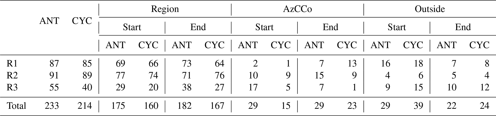
Along the AzCCo (Fig. 5), 75 % start within their region and 78 % end within it (not shown) (see Table 2 for more information). In R1, several cyclones originate north or west of Madeira Island, while anticyclones come from the northeast, and both structures present high relative frequencies to the southwest. In R2, most eddies originate locally, with only a few eddies tracked from outside the AzCCo. Cyclones have a clear preferential path to the southwest, but several migrate along the ridge. Preferred directions of anticyclones are to the west, with some along the ridge. West of the ridge, eddies originate in the north with a southwest path direction for most of the cyclones (see polar graphs). Only three cyclonic eddies originate in R2, which indicates that R3 is influenced by eddies' western origins related to the Gulf Stream extensions. The same occurs for anticyclones, with more eddies originating in R2. Based solely on path trajectories in R3, it could be hypothesised that resulting composites will be biased towards those of the large eddies associated with the Gulf Stream.

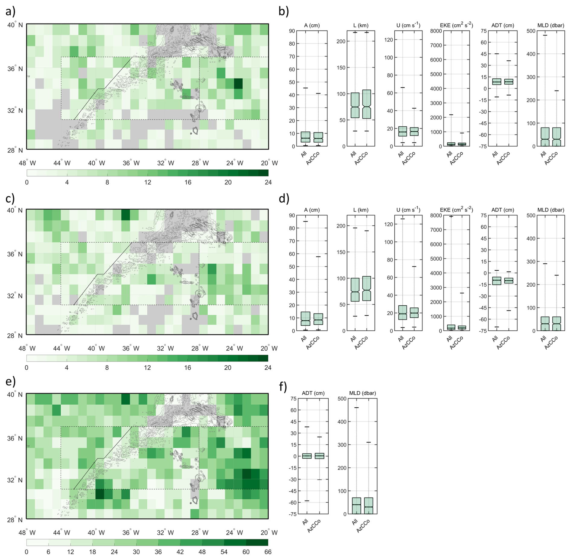
Figure 3 Number of Argo profiles in boxes of 1×1°. Emerged inside anticyclones (a), cyclones (b) and outside eddies (e) and their boxplots of kinematic properties for all region and inside the AzCCo: amplitude (A), radius (L), swirl velocity (U), eddy kinetic energy (EKE); absolute dynamic topography (ADT) and mixed layer depth (MLD) for anticyclones (b), cyclones (d) and ADT and MLD for Argo profiles emerged outside eddies (f). All refers to all eddies sampled in our study region, and AzCCo to those sampled only inside the AzCCo (R1 to R3).

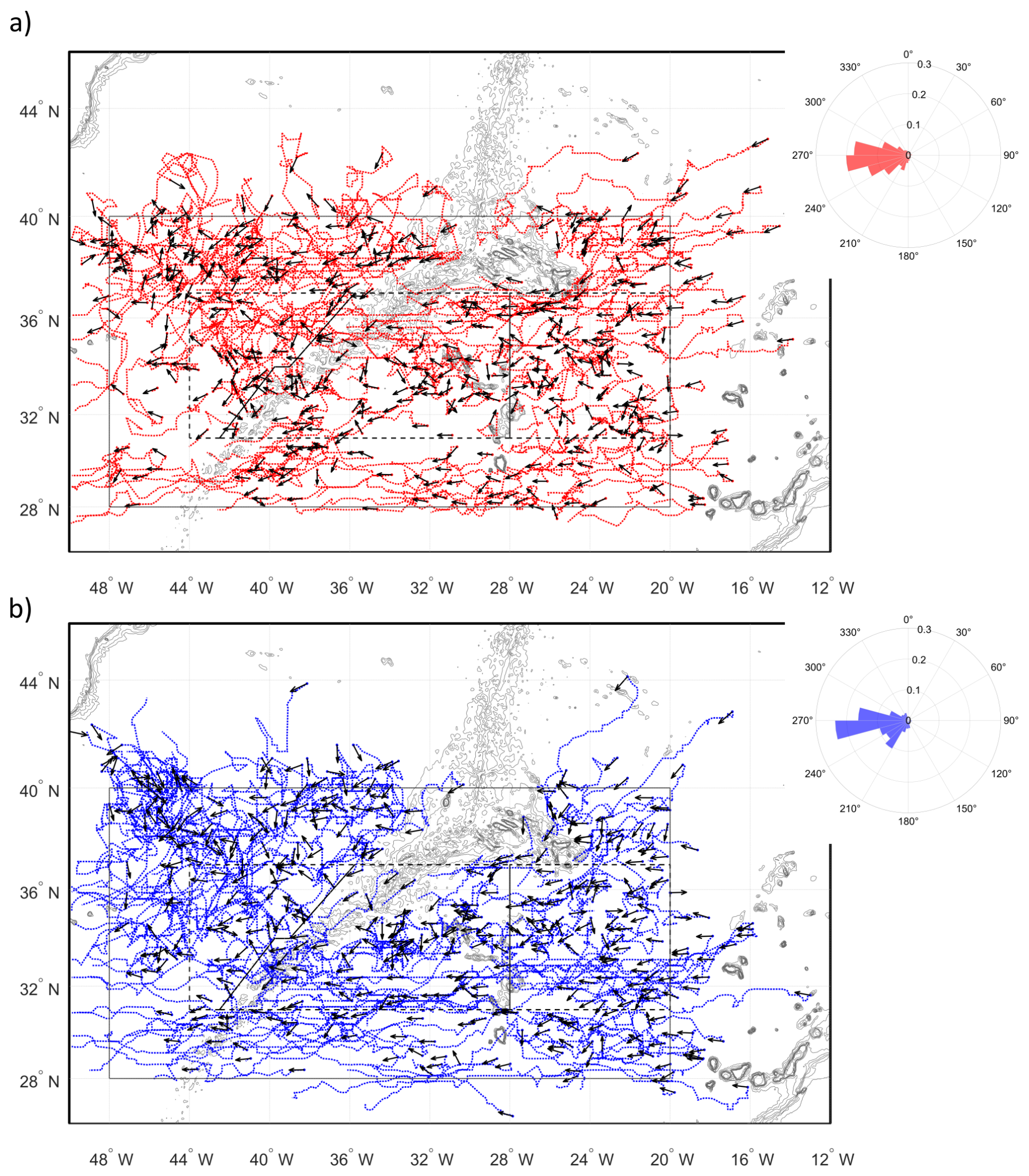
Figure 4 Trajectories (dotted lines) of eddies passing inside the study region (black box) for anticyclones (a) and cyclones (b). Beginnings of detection are represented by points, and the path direction by vectors. The dashed boxes are directly associated with the AzC corridor (AzCCo). The polar graphs represent the relative frequency in each class of the individual trajectory's azimuth, binned in 15° classes. The black box represents our study area, and the dashed boxes represent the regions associated with the AzCCo.

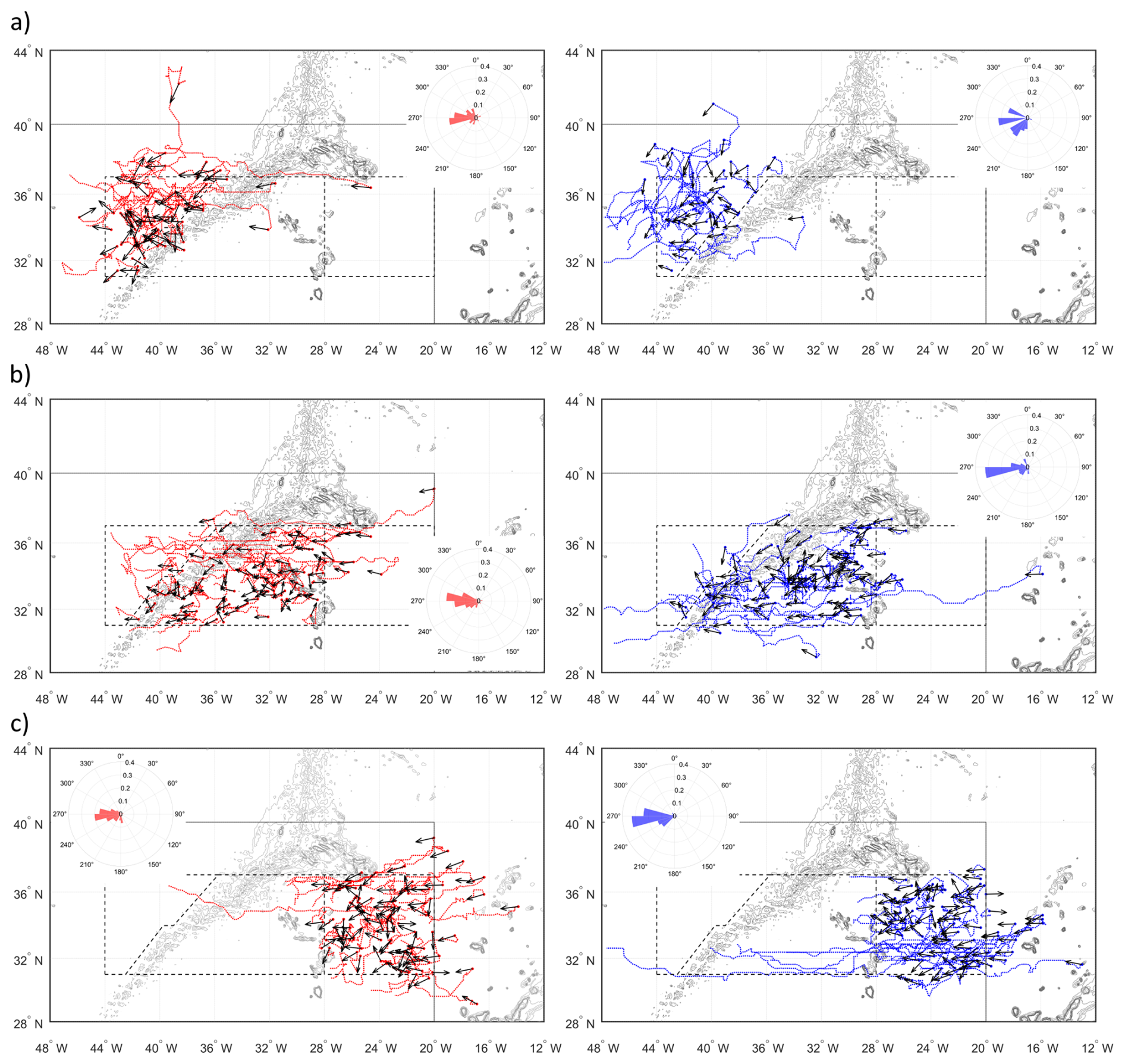
Figure 5 Trajectories (dotted lines) of eddies passing through the AzCCo in region 1 (a), region 2 (b), and region 3 (c) for anticyclones (left) and cyclones (right). Beginnings of detection are represented by points, and the path direction by vectors. The polar graphs represent the relative frequency in each class of the individual trajectory's azimuth, binned in 15° classes. The black box represents our study area, and the dashed boxes represent the regions associated with the AzCCo.

Table 2 Number of individual trajectories of anticyclones (ANT) and cyclones (CYC) that pass inside each region, with their start and end of detection inside each region, on the AzCCo and outside the corridor, respectively.

3.2 Mean zonal and meridional structure

The climatological meridional and zonal vertical mean structures for the Argo period reveal consistent patterns across the three regions along the AzCCo (Fig. 6a and b). A clear north–south deepening is evident in R1 and R2, associated with the Azores Front located around 34° N, characterised by colder and fresher waters to the north and warmer and saltier waters to the south. Its signature spans to depths of ∼ 750 dbar in CT and appears shallower in SA. In R3, a similar but less pronounced pattern is found. At ∼ 1500 dbar, the intrusion of colder waters (CT < 5 °C) enhances the vertical temperature gradient. A comparable behaviour is seen in the zonal mean, where temperature gradients increase from east to west.

The eastward penetration of Mediterranean Water (MW) is evident in the meridional SA mean of R1, marked by the intrusion of high-salinity waters below ∼ 1000 dbar near 20° W. In R2, a similar pattern is observed at the same depths, consistent with the westward propagation of MW, which is also visible in the zonal SA mean. A notable feature in R1 is the relative homogeneity of the salinity field between ∼ 750 and 1000 dbar. In R3, at ∼ 1500 dbar, the upwelling of fresher waters (SA < 35.3), together with lower temperatures, highlights the distinct characteristics between the eastern and western basins at depth.

It should be noted that the construction of the regional boxes influences the meridional means. In R2 (R3), areas west (east) of 40° W are more representative of the southern (northern) portion of the AzCCo, while areas east (west) of 40° W reflect more of the northern (southern) sector.

3.3 CT/SA vertical structure

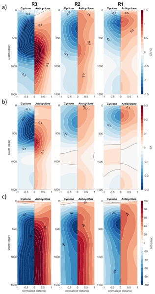
CT and SA composites along the AzCCo reveal the vertical structure of thermohaline anomalies associated with mesoscale eddies (Fig. 7). Meddy profiles were analysed separately to better isolate surface eddies; their vertical structure is discussed in Sect. 3.5. The internal structure asymmetry is observed both in CT and SA composites. The deflection of isotherms and isohalines downward (upward) from the centre of the composite to its boundary in the anticyclonic (cyclonic) case is visible, being more intense for the isohalines.

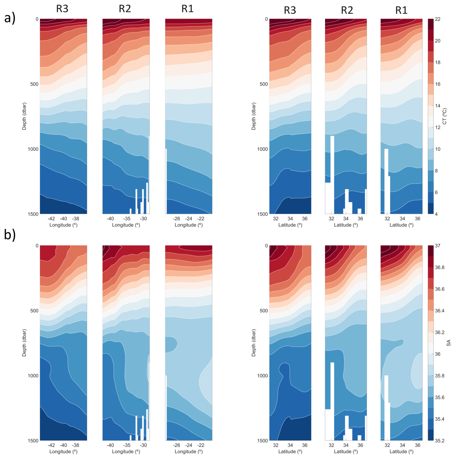
Figure 6 Mean WOA2018 climatology inside the three regions associated with the AzCCo for (a) CT and (b) SA. On the left are represented the meridional means and, on the right, the zonal. White represents the topography of the region associated with the SWSM chain and the shallower part of MAR.

From east to west, an intensification of the CT (Fig. 7a) vertical gradient between the east (R1 and R2) and the west (R3) of the ridge is observed, where colder waters (< 5 °C) can be observed at the 1500 dbar level, seen in both R3 anticyclones and cyclones and in R2 cyclones.

The SA composite (Fig. 7b) is highly asymmetrical between the two basins. R1 presents a layer of constant SA (∼ 35.8–35.7) ∼ 750 dbar thick in both sign structures, being deeper in anticyclones. This layer is also observed in R2, presenting less vertical span. R3 shows lower surface SA and intrusion of fresher waters (< 35.2) at the 1500 dbar level. The isohaline deflection is more pronounced in R3 with downwelling (upwelling) of around 75 dbar from the centre to the boundary in anticyclones (cyclones).

3.4 The isopycnal decomposition

The isopycnal decomposition reveals the respective contributions of heave (HEV), spice (SPI), and residual (RES) components to the vertical structure of CT and SA anomalies along the AzCCo, for both anticyclonic and cyclonic composites (Fig. 8).

A clear asymmetry between anticyclones and cyclones appears in both CT (Fig. 8a) and SA (Fig. 8b) anomaly structures, including differences in magnitude, vertical extent, and sign. Cyclones display a well-defined core, whereas anticyclones show a more vertically distributed structure throughout the water column, particularly in R2.

A systematic deepening of eddy cores is observed from east to west, with depths ranging from approximately 250–500 dbar for cyclones and 250–750 dbar for anticyclones. However, a reversal in polarity is evident: east of the MAR, cyclones are deeper than anticyclones, whereas in R3 the opposite pattern occurs, with anticyclones reaching the greatest depths (Fig. 8a and b). Anticyclones are characterised by warmer and saltier cores (> 0.75 °C and 0.1 salinity), while cyclones exhibit colder and fresher cores (< −2 °C and −0.3 salinity). In R1 for both structures, and in R2 for cyclones, a CT anomaly minimum occurs near 1000 dbar. At similar depths, SA anomalies reverse sign, reflecting depth-dependent changes in the background thermohaline structure linked to isopycnal displacement and highlighting the strong influence of stratification. In R2, anticyclones combine features of R1 and R3, forming a vertically stretched structure from the surface to about ∼ 1000 dbar. This reflects sampling above the ridge near the R3 boundary, indicating a transition in vertical structure along the AzCCo.

Anticyclones (cyclones) exhibit positive (negative) IVD (Fig. 8c), corresponding to the isopycnal surface deflection (elevation). This signal is stronger and more defined in cyclones (below −90 dbar in R1–R2 and −130 dbar in R3). In R1 and R2, the cyclonic IVD structure is similar, with a slight deepening of the maximum, while in R3, it becomes more vertically uniform between 400 and 1500 dbar. Anticyclones show comparable patterns across regions, more pronounced in R2 (> 80 dbar) and R3 (120 dbar). In all regions, IVD remains non-zero at 1500 dbar, indicating a deep-reaching, vertically coherent eddy signal.

HEV (Fig. 8d and g) dominates over SPI (Fig. 8e and h) in shaping CT and SA anomalies. HEV maxima occur slightly deeper than anomaly maxima and follow the same westward deepening trend. Furthermore, HEV shows the same sign as CT anomalies, while SA shows sign inversion due to reversal of the climatological gradient (∇X; Eq. 1) around 750 dbar, limiting the vertical extent of SA IVD. As for IVD, HEV remains non-zero at depth, supporting the presence of eddies extending below 1500 dbar.

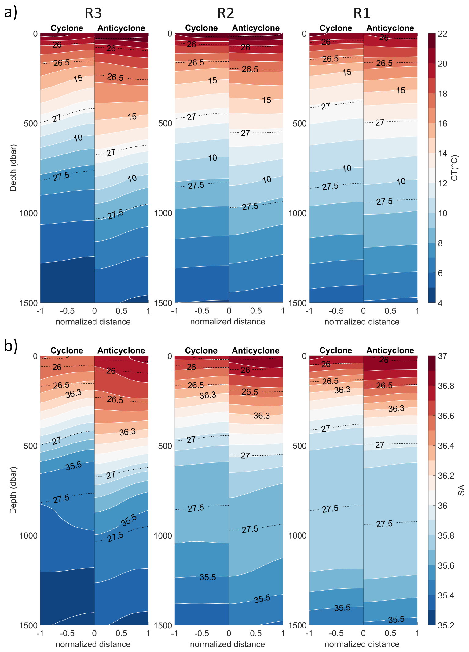
Figure 7 (a) CT radial vertical structure composite for sampled eddies inside R1, R2 and R3 for both anticyclonic and cyclonic structures. Dashed lines represent the density anomaly (kg m⁻³) relative to the surface. (b) The same as (a) but for the SA radial vertical structure composite.

The SPI structure (Fig. 8e and h) is more complex and confined to shallower depths. CT SPI shows higher eastern values restricted to the upper 250 dbar, with a sign inversion at depth and broader vertical extension. West of the MAR, anticyclones maintain consistent CT and SA sign, while cyclones exhibit a sign reversal near 1000 dbar. A similar pattern appears in SA SPI. This shallow confinement indicates that along-isopycnal variability is primarily surface-intensified in this region.

Although not a primary focus, ISOD residuals (Fig. 8f and i) are comparable in magnitude to SPI, suggesting contributions from diffusivity, diapycnal mixing, or processes such as eddy stirring not captured by HEV or SPI. This component is stronger in cyclones and west of the MAR.

Overall, the ISOD decomposition reveals a vertically structured eddy field dominated by heave-driven variability at depth and weaker, surface-intensified spice contributions, with clear regional and eddy-type asymmetries along the AzCCo. This highlights a vertical partitioning of thermohaline variability between deep and surface layers.

3.5 Median vertical structure

The 10 d mean translation of sampled eddies along the AzCCo reveals preferred directional pathways (Fig. 9a and b). Cyclones in R1 have mostly westward directions (255–285°), while anticyclones present a more dispersed path direction. Contrarily, in R2, anticyclones are westward, and cyclones have high relative frequencies to the west and southwest. An interesting aspect in R3 is that many eddies present southwest directions in both anticyclones and cyclones (higher in the cyclonic case), indicating a northern origin instead of eastern.

To compare the vertical structure of eddies in the AzCCo with background structure, medians of all profiles inside each region (Fig. 9c) were computed and compared to the median of the profiles emerging outside eddies (OUT profiles) for that region.

Asymmetry between anticyclones and cyclones is found along the corridor, being he CT anomaly medians always positive (negative) for anticyclones (cyclones) throughout the water column. Maxima are more defined in the cyclone case, with a deepening in the water column from east to west (from 250 to 600 dbar), and more intense west of the ridge. For anticyclones, their maximum varies from 250 to 750 dbar in the west, increasing also in intensity. In R2, the CT anomaly vertical profile is more uniform than the two other regions.

From east to west, the SA median zero deepens from ∼ 750 dbar in R1 to ∼ 1000 dbar in R3 for both structures. Being associated with the MW presence, it is visible across the AzCCo and followed by an inversion of the SA anomaly's cyclone sign (from negative to positive) in R1. The same inversion is observed in anticyclones with less intensity, resulting from the downwelling of the MW upper boundary by the anticyclone's internal deflection of the isopycnal surfaces. The same vertical pattern towards zero is exhibited by the CT anomaly in R1, but without the inversion of its median.

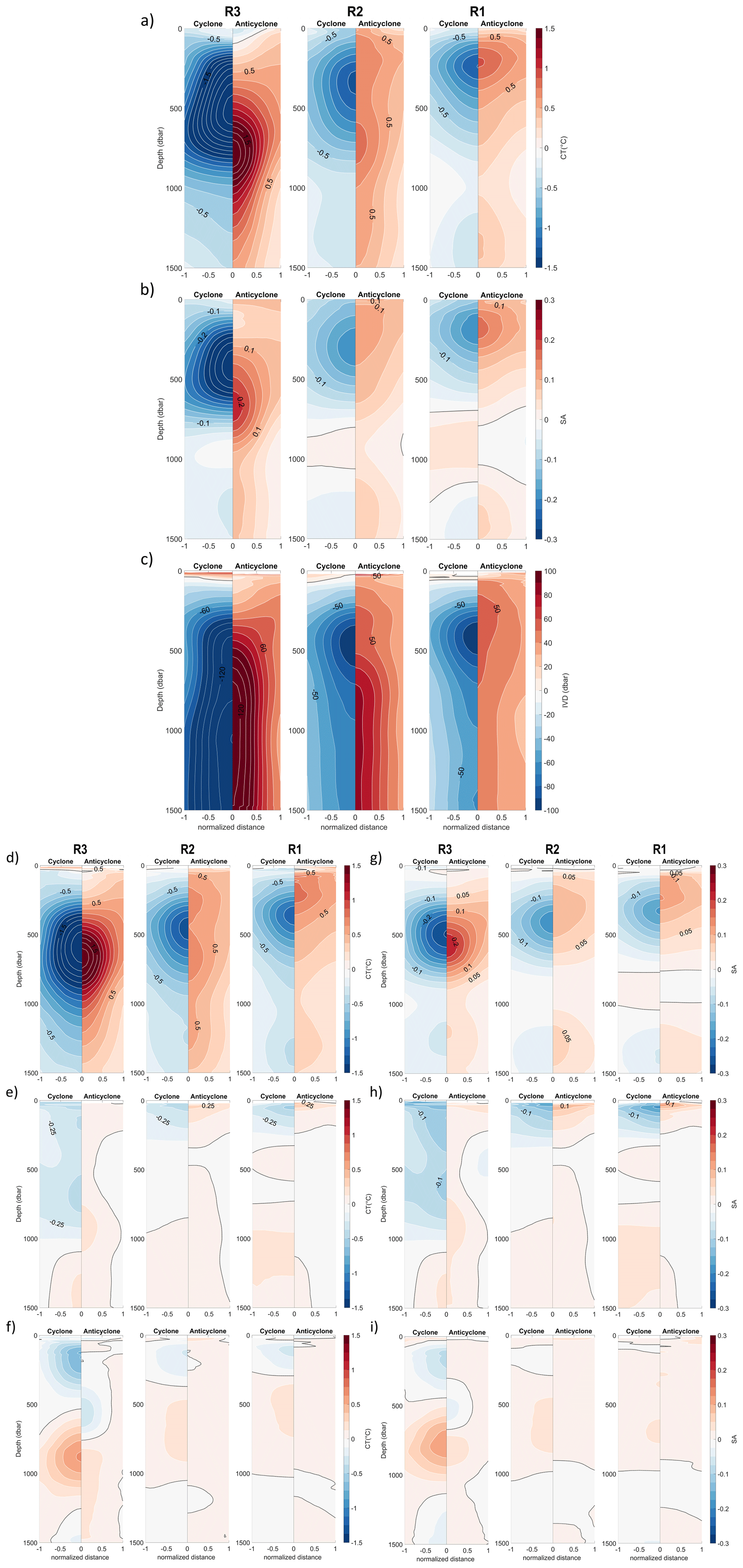
Figure 8 ISOD decomposition: radial vertical structure composite for sampled eddies inside R1, R2 and R3 for both anticyclonic and cyclonic structures. (a) CT anomaly, (b) SA anomaly, (c) Isopycnal Vertical Displacement (IVD). The dotted black line contour represents zero for that variable. ISOD decomposition: radial vertical structure composite for sampled eddies inside R1, R2 and R3 for both anticyclonic and cyclonic structures. (d) CT HEV, (e) CT SPI, (f) CT RES, (g) SA HEV, (h) SA SPI, (i) SA RES. The dotted black line contour represents zero for that variable.

The IVD median's vertical structure is almost homogeneous for the anticyclones from the surface to the 1500 dbar, indicating that their internal structure is more uniform, which in R1 and R2 presents a maximum above the 500 dbar level. As for CT, the IVD sign is always positive (negative) in anticyclones (cyclones) in all regions, which indicates that the eddies' presence influences the water column to the 1500 dbar. Furthermore, as IVD medians are still significant, as well as their 90th percentiles (∼ 100 dbar in R1 and R2 and ∼ 200 dbar in R3), meaning that these structures have an influence that can reach depths below that level.

OUT medians for CT and SA anomalies are zero along the AzCCo in the water column, though their percentiles still present significant values (the shaded area of the percentiles is not shown in the figure). This could indicate processes associated with meanders and/or filaments that are not captured by the eddy detection algorithm; virtual eddies (see Sect. 2.4); or even being associated with other processes like Rossby waves.

As meddies have a well-known vertical structure, which helped us to better understand the SPI and HEV concepts and are therefore analysed in this section. The sampled meddies south of 38° N usually present, with some exceptions, western directions (Fig. 10a), while those north of that latitude exhibit southwest directions. These meddies are grouped according to their sign at the surface, as the Argo float emerged inside a surface cyclone or anticyclone. A major difference emerges from their vertical structures (Fig. 10b): while cyclones are colder and fresher until the 600 dbar depth, anticyclones show a slightly warmer and saltier structure at those depths. Below that level, all present warmer and saltier structures to the 1500 dbar depth, with anticyclones presenting higher anomalies (4 °C and 0.8 of salinity against 1 °C and 0.25 of salinity) with shallower maximum, while cyclones' median is more constant at depth. The asymmetrical structure of the IVD; anticyclones show clearly high positive values, while cyclones have mainly negative ones, could indicate that we are both in the presence of anticyclonic meddies (positive IVD) and cyclonic meddies (negative IDV). The sampling of meddies by these profiles is corroborated by the CT-SA diagrams (not shown), where higher values of CT and SA are observed, conforming with those associated with meddies. Furthermore, the 10th percentile of the cyclones' IVD presents a sign change at around 1000 dbar, which could indicate that some of these profiles sampled anticyclonic meddies.

4 Discussion

4.1 West-east eddies' origins

Zonal differences in the eddies' vertical structure along the current main axis are more pronounced between the east and west of MAR, as the ridge acts as a boundary for two areas with very distinct dynamics. From east to west, a deepening of the anomaly's maxima, accompanied by increased intensity (from > 0.5 °C and 0.1 in salinity to 1.5 °C and 0.2 in salinity) and vertical extension (from 750 to 1250 dbar), is observed both in the 2D radial composites and in the median vertical structure. Anticyclones present warmer, saltier cores, while cyclones have cold, fresh cores with a clear, well-defined maximum.

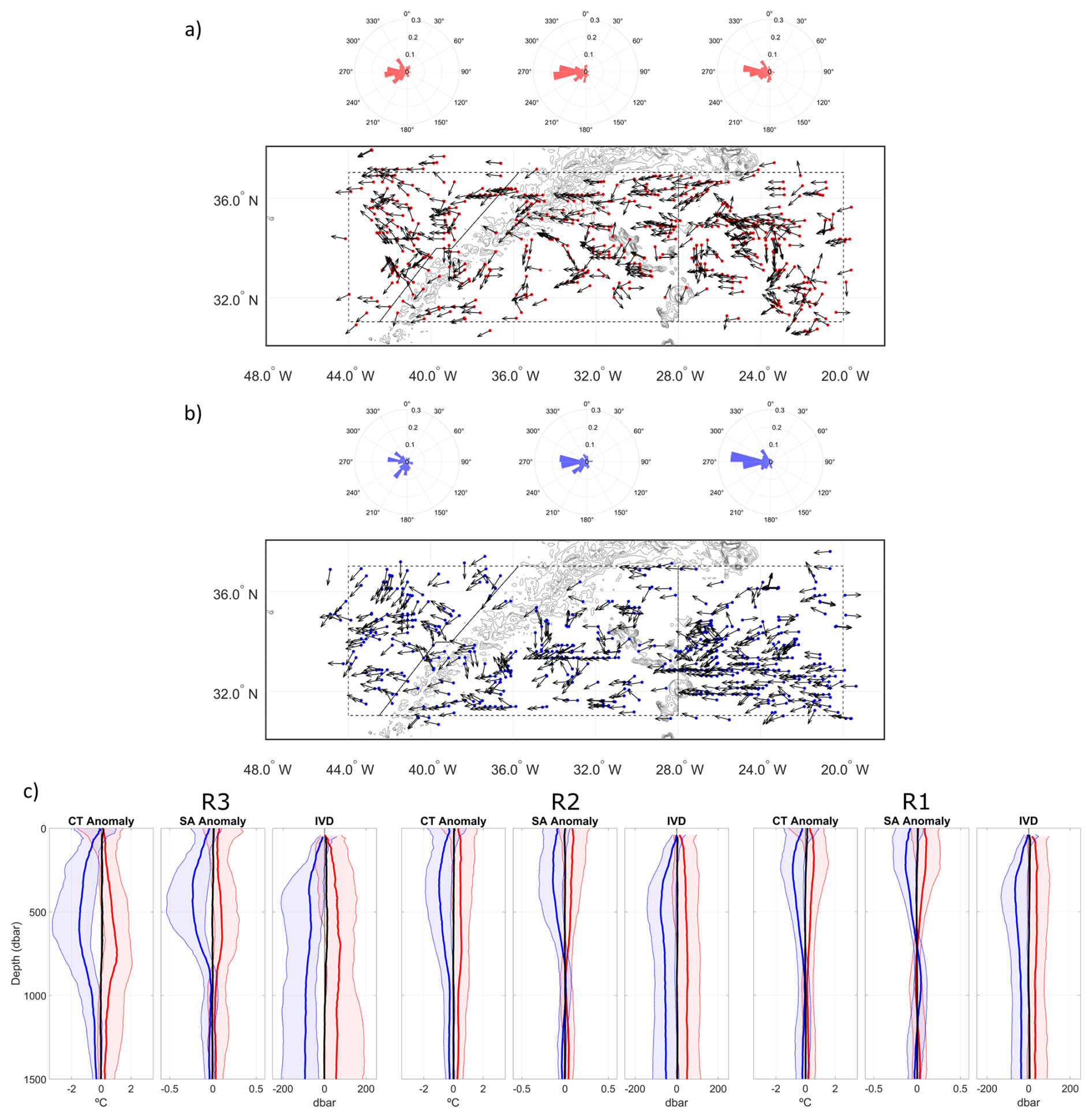
Figure 9 (a) Map of the general direction path (10 d mean) of the sampled eddies along a trajectory inside each region. Location of the sampled eddies represented by points and the path direction by vectors. The polar graphs represent the relative frequency in each class of the individual trajectory's azimuth, binned in 15° classes. (b) Median vertical structure of the eddy composite for both sign structures (anticyclone red and cyclone blue) and the median vertical structure of the outside eddies (black) for the three regions associated with the AzCCo: R1 (right), R2 (centre), and R3 (left) for the CT and SA anomalies and the vertical displacement, IVD. 

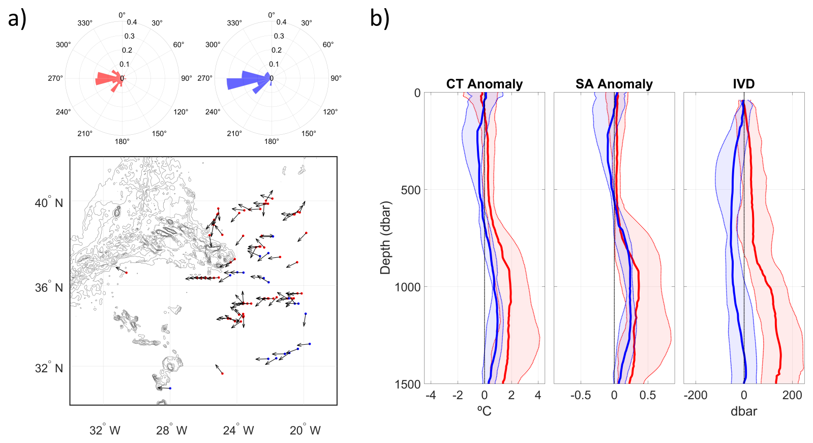
Figure 10 (a) Map of the general trajectories of the sampled meddies (anticyclones red and cyclones blue) for a period of 10 d. The polar graph represents the relative frequency in each class of the individual trajectory's azimuth, binned in 15° classes. (b) Median vertical structure of the meddies' profiles for both sign structures (anticyclone red and cyclone blue) for the CT and SA anomalies and the vertical displacement, IVD.

The R1 eddy composite is predominantly local, with some originating in the northeast of the AzP in the anticyclonic case and north of Madeira Island for both structures. In the latter case, these eddies may have two possible origins: either from the evolution of AzC meanders, leading to the formation of eddies that propagate westward, or from the interaction of those with eddies originating in the Canary Upwelling System, which can propagate westward to longitudes as far as 40° W, as previously reported by Pegliasco et al. (2015) and Sangrà et al. (2009). In R3, the sampled trajectories indicate translation from the north and east, primarily in the cyclonic case. Furthermore, a migration of eddies to the south on the western flank of the ridge is observed both on the global and the sampled trajectories' azimuths. Ollitrault and Colin de Verdière (2002) reported, based on the trajectories of SOFAR floats launched on each side of the ridge, that eddies are frequently found to travel southward along the western ridge's flank. However, they also found that, after the floats span the western basin between 30 and 45° N, eddies are also found to travel towards the ridge. Furthermore, Caldeira and Reis (2017), using eddy trajectories tracked on altimetry data (Chelton et al., 2011) and the computation of the zonal and meridional Ekman transport, reported that the Azores Archipelago (in this work represented in the northwest, centre, and southeast of the AzP) is a confluence zone of far-field eddies with different origins. The north-western and central regions are predominantly influenced by the Gulf Stream, filaments, meanders, and eddies, while the south-eastern region is impacted by eddies that are likely to have originated from the meandering AzC pinching. This is consistent with the hypothesis that eddies in R3 are primarily a byproduct of the merging and splitting of mesoscale structures with different origins: those generated in the east and crossing the ridge, and those generated by the evolution of the Gulf Stream branches, migrating to the south along the western flank of the ridge. R2 is a transitional region encompassing the MAR, with eddies originating on both sides of the ridge and above it. The composite vertical structure of eddies in this region exhibits characteristics of both R1 and R3, presenting an elongated core that spans nearly the entire water column. This structure reflects the shallower cores of R1 as well as the deeper cores of R3, influenced by the presence of eddies that may originate from the Gulf Stream system.

4.2 HEV vs SPI

HEV dominates the vertical structure of both CT and SA anomalies on both sides of the MAR throughout most of the water column, with SPI exhibiting higher values in the upper ∼ 250 dbar east of the MAR and a larger vertical extension west of the ridge. In R1 and R2, HEV presents well-defined maxima for anticyclonic (cyclonic) structures around the 400 dbar (500 dbar) level, indicating that the observed anomalies are primarily driven by the vertical displacement of isopycnal surfaces. This mechanism leads to the depression (elevation) of isopycnal surfaces and the associated downwelling (upwelling) of warmer (colder) waters, resulting in warm (cold) anomalies. West of the MAR, the same dynamical behaviour is observed, but with stronger amplitude and greater vertical extent, consistent with larger IVD values in this region. This dominance of HEV indicates that eddy-induced thermohaline anomalies along the AzCCo are primarily governed by vertical redistribution processes (eddy pumping), rather than by lateral transport of distinct water masses along isopycnal surfaces.

The generally low SPI values observed across the AzCCo suggest that thermohaline anomalies are not primarily driven by contrasts along isopycnal surfaces within most eddies. This can be explained by the fact that many eddies evolve within the corridor, where background CT and SA gradients are relatively smooth in the zonal direction. As a result, advection along isopycnal surfaces introduces only minor deviations from the background state. An exception is found for meddies (not shown), which advect MW, leading to significantly higher SPI values. Furthermore, the weak SPI signal implies a limited efficiency of these eddies in transporting tracers over long distances, reinforcing the view that their primary role is the vertical redistribution of properties. In this sense, the AzCCo can be viewed as a regime where the surface-intensified mesoscale variability is dominated by deformation of the background stratification rather than by the advection of thermohaline properties.

These results are consistent with the conceptual framework of eddy-driven transport mechanisms. Four main processes are typically identified: eddy pumping, eddy trapping, eddy-induced Ekman pumping, and eddy stirring. At a global scale, He et al. (2024) show that temperature anomalies are primarily controlled by eddy pumping, consistent with the dominance of HEV in our results. In contrast, eddy trapping becomes relevant in regions with strong horizontal property gradients, as highlighted by Frenger et al. (2015). In our study area, this mechanism is most clearly expressed in meddies, where sharp zonal gradients in temperature and salinity lead to enhanced SPI values. Regional studies further support this interpretation. Keppler et al. (2018) and He et al. (2023) show that eddy trapping tends to dominate near the surface, whereas eddy pumping becomes increasingly important at depth. Similarly, Amores et al. (2017) found that temperature and salinity anomalies are mainly driven by advection in the upper ∼ 200 m, while vertical displacement of isopycnal surfaces dominates below ∼ 300 m. Their reported signal extending down to ∼ 1200 m is consistent with the non-vanishing HEV, and the high IVD values observed throughout the AzCCo east of the MAR. In situ studies by Pingree et al. (1996) and Mouriño et al. (2003) also report deep-reaching eddy signatures extending from several hundred meters to full water column depth, supporting the presence of vertically coherent eddy structures in the region.

The westward intensification of HEV reflects a transition between two dynamical regimes separated by the MAR: an eastern region more influenced by local stratification and horizontal gradients, and a western region characterised by deeper, more energetic eddies with a capacity to redistribute properties throughout a larger fraction of the water column.

Finally, the dominance of HEV has important implications for vertical exchanges in the region. Cyclonic eddies, through isopycnal upwelling, are likely to enhance the upward transport of colder, nutrient-rich waters, while anticyclones promote downwelling and subduction of surface waters. Given the deep vertical extent of HEV observed here, these processes are not confined to the upper ocean but may contribute to the ventilation and redistribution of properties down to at least 1500 dbar along the AzCCo.

5 Conclusions

In this study, we analysed the CT and SA profiles of Argo floats that emerged within tracked eddies identified from ADT maps. From the total of individual sampled eddies, 617 anticyclones and 593 cyclones were profiled in the AzCCo. The main objective was to characterise the vertical structure of mesoscale turbulence along the AzCCo and to understand its impact on the water column. Our findings can be summarised as follows.

The vertical structure differences found between the eastern and western sides of the ridge are associated with the origins of the sampled eddies: while in the east, most eddies originate locally, in the west, the majority originate outside R3, representing a combination of eddies propagating from the east and from the northwest, the latter being associated with Gulf Stream eddies. This results in more intense anomalies in the westward composites.

When analysing the HEV and SPI signatures and intensities, we concluded that: (1) The HEV component is the main contributor to the formation of the CT and SA anomalies, as it exhibits the highest values along the AzCCo. (2) This dominance indicates that most eddy anomalies are generated through an eddy pumping mechanism, producing warm and saltier (cold and fresher) anomalies due to the downwelling (upwelling) of the shallower (deeper) isopycnal surfaces in the anticyclonic (cyclonic) eddy interior. (3) SPI shows lower values across the domain, although slightly higher values are found in the upper 250 dbar east of the MAR, reflecting the tendency of eddies to trap different water masses.

Regarding the influence of mesoscale turbulence on the water column, this work shows that: (1) From east to west, the absolute maximum values of both CT and SA anomalies occur at increasing depths, from ∼ 250 to ∼ 750 dbar. (2) Anticyclones exhibit a more uniform structure while cyclones display a well-defined subsurface maximum. (3) IVD absolute values exceeding 50 dbar down to 1500 dbar confirm the deep-reaching influence of both anticyclonic and cyclonic eddies. (4) High IVD absolute values (above 150 dbar) across the AzCCo further indicate that these structures could have the potential to enhance vertical advection not only of heat and salt, but also of biogeochemical properties.

Overall, this study confirms that mesoscale eddies along the AzCCo exert a deep influence on the water column, with differences in their vertical structure linked to eddy origins and dynamical properties. Taken together, these results depict the AzCCo as a vertically driven mesoscale regime in which eddies primarily act through isopycnal displacement, redistributing thermohaline properties over a large fraction of the water column rather than through lateral transport. This has important implications for regional ocean dynamics, suggesting that mesoscale processes in this corridor may play a key role in deep ventilation and in the vertical redistribution of heat, salt, and biogeochemical tracers.