Data-driven enhancement of ocean surface forcing for accurate floating debris transport modelling in the East/Japan Sea

Floating debris transport in marginal seas is controlled by a combination of geostrophic currents, wind-driven currents, wave-induced drift, and direct wind forcing, but the relative importance of these processes remains difficult to quantify without in-situ trajectory observations. This study evaluates near-surface forcing combinations for particle tracking in the East/Japan Sea using 33 GPS-tracked surface drifters deployed off the Korean coast in November 2021. The drifters revealed a clear cross-basin transport pathway toward the Japanese coastline and an early bifurcation near a hyperbolic-type Lagrangian structure. We used a particle tracking model to test combinations of geostrophic current, Ekman current, Stokes drift, and windage against the observed drifter trajectories using MAE and NCLS metrics. For undrogued DX drifters, the best performance was obtained by combining geostrophic current, Stokes drift, and windage. For drogued DO drifters, which sampled a deeper effective depth, the inclusion of all four forcing components provided the best agreement with observations. The optimized forcing combinations outperformed benchmark simulations driven by the GOFS analysis and GLORYS reanalysis in this specific event, primarily because they better reproduced the Lagrangian structure associated with the early trajectory bifurcation. Seasonal simulations showed that winter winds enhance eastward transport and beaching along Japan, whereas weaker summer winds allow mesoscale eddies to broaden particle dispersion. The present framework represents the fluid-dynamical component of near-surface particle transport and does not explicitly include plastic-specific fate processes such as fragmentation, biofouling-induced buoyancy changes, aggregation, settling, or resuspension.

1 Introduction

Millions of tons of plastic debris enter the ocean annually, posing a significant threat to marine ecosystems and human health. This debris accumulates in eddies and gyres (Lebreton, 2022; Maximenko et al., 2012; Thiel et al., 2018), washes ashore on coastlines (Chenillat et al., 2021; Cole et al., 2011; Cózar et al., 2014; Dobler et al., 2022; Nakakuni et al., 2024), and fragments into smaller pieces that disperse widely over time. These fragments pose serious risks to marine life through ingestion, particularly for species with vast foraging and migration ranges (Clark et al., 2023; Santos de Moura and Vianna, 2020). Because plastic debris can facilitate disease transmission, damage critical habitats like coral reefs (Pinheiro et al., 2023), impact human health (Paul et al., 2024), disrupt food chains (Saeedi, 2024), and alter ecosystem dynamics (Tekman et al., 2022), accurate modeling to track the trajectories, distributions, and accumulation of floating plastic debris is urgently needed.

Particle Tracking Models (PTMs) have been widely implemented to model the transport and fate of floating materials (Lebreton et al., 2012; Onink et al., 2019). Such models have also been extended to study plastic debris dispersion in rivers discharging into the Indian Ocean (Irfan et al., 2024). Within marginal seas, PTM applications include tracking floating particle trajectories influenced by subsurface currents in the Gulf of Mexico (Liang et al., 2021), modeling oil particle pathways following the Deepwater Horizon oil spill (Mariano et al., 2011), tracking plastics in the Mediterranean Sea using surface currents and Stokes drift (Liubartseva et al., 2018), predicting particle trajectories in the Adriatic Sea (Castellari et al., 2001), simulating oil spill diffusion in the Sea of Okhotsk (Ono et al., 2013), and predicting surface debris movement in the East/Japan Sea (EJS) (Iwasaki et al., 2017).

PTMs are typically driven by Eulerian surface currents, which are heavily influenced by a combination of geostrophic currents, Ekman transport, Stokes drift, and windage (Röhrs et al., 2023; Van Sebille et al., 2020). Geostrophic currents, resulting from the balance between the Coriolis force and horizontal pressure gradients (Sudre et al., 2013), play a fundamental role in long-term ocean circulation and influence both surface and subsurface flows globally. Wind directly affects floating objects by exerting force on their exposed surface area, known as windage, often quantified by wind drift factors ranging from 0 % to 5 % of the wind speed (Gu et al., 2024; Tamtare et al., 2022). Ekman transport, driven by wind stress and the Coriolis effect, generates a vertical current profile within the upper ocean layers (Bressan, 2019) and has been linked to microplastic accumulation in subtropical regions (Onink et al., 2019). Stokes drift is a wave-induced Lagrangian drift that adds to the Eulerian surface current and therefore contributes directly to the transport of floating objects (Mao and Heron, 2008; Tamtare et al., 2022). Consequently, a systematic study determining which physical processes dominate particle movement is crucial for model accuracy.

Drifter experiments are an essential tool for evaluating PTM results that simulate the transport and dispersion of floating plastic debris and the corresponding physical processes on the ocean surface. In open oceans, validation is often supported by massive datasets such as the Global Drifter Program, which maintains thousands of drifters globally (Lumpkin et al., 2017; Maximenko et al., 2012). With the exception of the massive CODE-type drifter experiment in the Gulf of Mexico (Poje et al., 2014; D'Asaro et al., 2018), drifter experiments in marginal seas are typically constrained in scale, often relying on a small number of drifters to investigate local transport features. For instance, recent studies in the North Sea used only 6 to 12 drifters to validate surface transport models (Callies et al., 2017; Medina-Rubio et al., 2026), and similar process-oriented studies in the East China Sea were conducted with as few as 4 to 29 SVP-type drifters (Hsu et al., 2021; Sun et al., 2022). Sotillo et al. (2016) compiled a CODE-type drifter dataset in the Strait of Gibraltar to validate ocean models and track contaminants. The primary role of these experiments is to validate the surface currents that directly affect the accuracy of the debris tracking model. However, many tracking model studies in marginal seas still lack validation with in-situ drift data, or employ drifter types that are not suitable for tracking floating debris. Here, we utilized 33 surface drifters deployed simultaneously, tracking currents at a depth of 0.3 m. Although this number is smaller than open-ocean campaigns, it represents one of the largest synoptic datasets conducted in a marginal sea and constitutes the largest surface drifter experiment conducted in the EJS.

We investigate transport and dispersion in the EJS using PTMs validated with drifter experiments. The EJS, a marginal sea approximately 1000 km wide, is a recognized “hot spot” for microplastic accumulation (Isobe et al., 2015; Kuroda et al., 2024) and is often described as a “miniature ocean” due to its encapsulation of major global oceanic processes, such as deep water formation, thermohaline circulation, and mesoscale eddy activity, within a relatively small and semi-enclosed basin (e.g., Ichiye, 1984; Kim et al., 2001; Talley et al., 2006). Bordered by the Korean Peninsula, Japan, and the Russian Far East, the EJS receives a mix of natural and anthropogenic materials, including plastic debris, transported by ocean currents such as the Tsushima Warm Current, a branch of the Kuroshio Current flowing from the East China Sea, as well as by wind (Park and Seo, 2021). Although the transport and distribution of plastic debris in the EJS have been studied (Iwasaki et al., 2017; Kim et al., 2021; Takeda and Isobe, 2024), there remains a lack of observational data in this marginal sea to validate particle trajectories and the specific physical processes influencing near-surface particle movement in the region.

In this study, we aimed to optimize the near-surface forcings that govern floating debris transport using a PTM validated with in-situ surface drifter observations. Here, “floating debris transport” refers to the fluid-dynamical transport component represented by passive particles moving near the ocean surface rather than the complete fate of specific macroplastic or microplastic particles. A drifter experiment was conducted to trace near-surface transport and assess the accuracy of simulated particle trajectories. In the results section, we identify the optimal combinations of key surface forcing components – geostrophic currents, Stokes drift, Ekman currents, and windage – for accurately modeling floating debris transport. By incorporating these forcings into the PTM, we simulated particle trajectories and compared them with observed drifter paths. Particle-specific processes such as fragmentation, biofouling-induced buoyancy change, aggregation, settling, and resuspension were not included in the present framework. This simplification is appropriate for the present objective because the simulated transport time scale is less than three months, whereas fragmentation has been reported to act on much longer, decadal time scales and to have little influence on large-scale microplastic transport over periods shorter than three years (Onink et al., 2022). In the discussion section, we evaluate the performance of the optimized forcing combinations relative to ocean analysis/reanalysis velocity products and further apply these combinations to estimate the seasonal variability of surface transport and beaching patterns of floating debris in the EJS.

2 Materials and methods

2.1 Drifter experiment

Custom-made cylindrical drifters (Fig. 1a) were used to observe near-surface currents by tracking their movements in the EJS. The drifters, equipped with GPS trackers, were designed to collect location data at 5 min intervals over several months. Each drifter measured 30 cm in height and 9 cm in diameter, with the top 3–5 cm protruding above the water surface when deployed. A total of 33 drifters were deployed, consisting of 23 undrogued drifters (hereafter referred to as DX drifters) and 10 drogued drifters (hereafter referred to as DO drifters). The drogue for the DO drifters consisted of two 30 cm × 30 cm plastic plates arranged perpendicularly and positioned at a depth of 2 m. By using surface drifters with slightly different depths, we aimed to investigate near-surface transport processes relevant to floating marine debris. Drifter positions were tracked from deployment until either beaching occurred or the signal was lost. The mean, minimum, maximum, and standard deviation of drifter lifetimes were 48.05, 12.2, 79.7, and 22.4 d, respectively. The location data were interpolated at 15-minute intervals and used for subsequent analysis. The DX and DO drifters were used to sample near-surface transport, but they were expected to respond differently to wind forcing. The DX drifter had a small part exposed above the sea surface, so it could be more affected by direct wind forcing and Stokes drift (Niiler and Paduan, 1996; Röhrs et al., 2012).

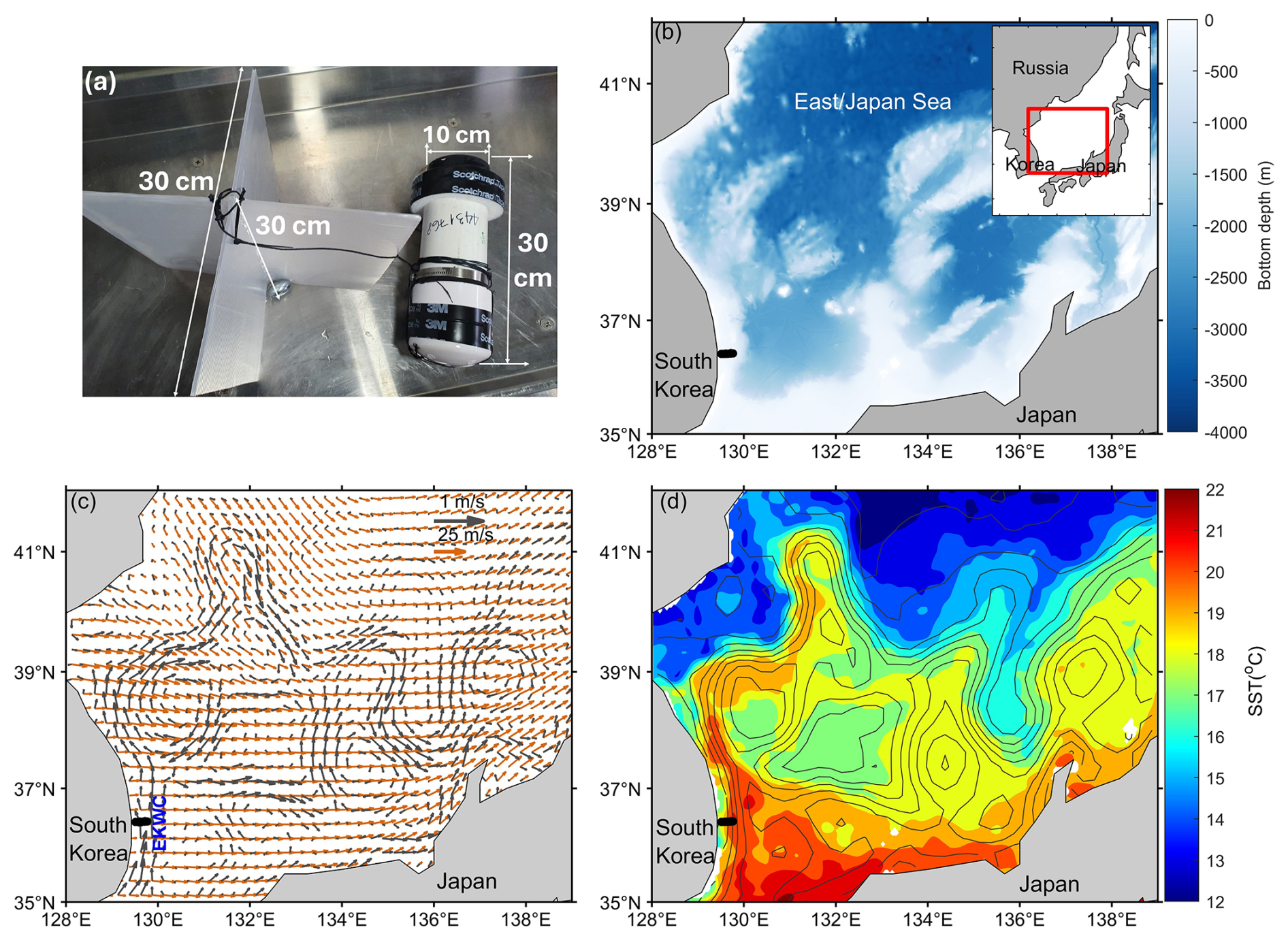
Figure 1 (a) Photograph and dimensions of the undrogued DX and drogued DO drifters. (b) Bathymetry of the East/Japan Sea, with the inset showing the surrounding geographic region. (c) Geostrophic current vectors (black) and 10 m wind velocity vectors (orange), both averaged over the first week after drifter release. The East Korea Warm Current (EKWC) is indicated in blue, and the reference vectors are shown in the upper-right corner. (d) Sea surface temperature (SST; color shading) and sea surface height (SSH; contour lines), both averaged over the first week after drifter release. Thick black lines indicate the initial drifter deployment locations.

In contrast, the DO drifter included a 30×30 cm drogue centered near 2 m depth to increase submerged drag and reduce direct wind slippage, following the general water-following principle of drogued surface drifters such as CODE and CARTHE drifters (Davis, 1985; Novelli et al., 2017). CARTHE drifters sample the upper approximately 0.6 m with wind-induced slip less than 0.5 % of the 10 m wind speed, whereas CODE drifters sample the upper meter with reported downwind slip of about 0.1 % of the wind speed (Poulain and Gerin, 2019; Poulain et al., 2022). Thus, the DX and DO drifters are treated here as custom observational benchmarks with different effective depths and windage sensitivities, rather than as exact equivalents of CODE or CARTHE drifters.

We deployed the drifters across the East Korea Warm Current (EKWC) region in the EJS (Fig. 1). The circulation along the eastern Korean Peninsula is primarily influenced by the northward-flowing EKWC and the southward-flowing North Korean Cold Current (NKCC), both of which are modulated by coastal currents, mesoscale eddies, and frontal structures (Lee and Niiler, 2010). These flow systems generate complex near-surface transport pathways as drifters interact with regional oceanographic features (Prants et al., 2011; Onink et al., 2019). The drifters were released at six deployment locations near the Korean coast, with four DX drifters and either one or two DO drifters released at each location. The deployment started on 10 November 2021 at 01:40 UTC, and the subsequent groups were released at intervals over approximately 3 h. The one-week-averaged geostrophic current and 10 m wind velocity fields after drifter release are shown in Fig. 1c, together with the initial drifter location (black line). During this period, a strong northward geostrophic current was present along the Korean coast, while the 10 m wind field was predominantly eastward to northeastward over the deployment region. The corresponding one-week-averaged sea surface temperature (SST) and sea surface height (SSH) fields are shown in Fig. 1d, indicating mesoscale variability and frontal structures in the EJS. In particular, the mesoscale eddy evident near the drifter release locations likely influenced the subsequent pathways and final fates of the drifters.

2.2 Current data sets

Four current components were considered to be associated with the movement of drifters: geostrophic current (Sudre et al., 2013; Tamtare et al., 2022), Ekman current (Sudre et al., 2013; Huang et al., 2021), Stokes drift (Curcic et al., 2016; Iwasaki et al., 2017; Pärn et al., 2023), and windage (Gu et al., 2024). Geostrophic current (u_G or G), representing the background horizontal velocities, was obtained from the SEALEVEL_GLO_PHY_L4_MY_008_047 dataset. This dataset is a Copernicus Marine SEALEVEL Level-4 altimeter product processed by the CNES/CLS DUACS system. It combines multi-mission satellite altimeter observations, including Sentinel-6A, Sentinel-3A/B, Jason-3, SARAL/AltiKa, CryoSat-2, OSTM/Jason-2, Jason-1, TOPEX/Poseidon, Envisat, GFO, ERS-1/2, and Haiyang-2A/B. The current version of the product provides daily global ocean observations at a nominal spatial resolution of 0.125° and a temporal resolution of 1 d. For the particle-tracking calculations, the velocity fields were processed on the originally prepared computational grid with a grid spacing of approximately 0.25°, corresponding to about 25 km in the EJS. Wind velocity at 10 m above the sea surface (u₁₀) was obtained from the ECMWF Reanalysis v5 (ERA5) dataset, with a spatial resolution of 1/4° and a temporal resolution of 1 h. The wind data were converted to wind stress using the bulk formula (τ=ρ_aC_du₁₀|u₁₀|), where ρ_a is the air density, and $C_{\mathrm{d}}(={\mathrm{10}}^{-\mathrm{3}}(\mathrm{0.8}+\mathrm{0.065}\left|{\mathit{u}}_{\mathrm{10}}\right|)$) is the drag coefficient (Chen et al., 2020; Wu, 1982; Cushman-Roisin and Beckers, 2011; Rypina et al., 2021).

The windage velocity, u_W, was parameterized as u_W=ru₁₀, where r is the windage coefficient and u₁₀ is the wind velocity at 10 m height. The coefficient r was estimated using a first-order balance between aerodynamic drag on the exposed part of the drifter and hydrodynamic drag on the submerged part:

$$\begin{array}{}\text{(1)}& r=\sqrt{{\displaystyle \frac{{\mathit{\rho }}_{\mathrm{a}}{C}_{\mathrm{d},\mathrm{a}}{A}_{\mathrm{a}}}{{\mathit{\rho }}_{\mathrm{w}}{C}_{\mathrm{d},\mathrm{w}}{A}_{\mathrm{w}}}}},\end{array}$$

where ρ_a and ρ_w are the densities of air and seawater, C_d,a and C_d,w are the drag coefficients in air and water, and A_a and A_w are the projected areas above and below the sea surface, respectively (Isobe et al., 2011). Because C_d,a and C_d,w were not measured directly for the custom drifters, we first assumed $C_{\mathrm{d},\mathrm{a}}/C_{\mathrm{d},\mathrm{w}}\approx \mathrm{1}$ as a geometry-based first-order approximation, consistent with previous studies (de Dominicis et al., 2016; van der Mheen et al., 2020). This assumption is appropriate for the DX drifters because the exposed and submerged parts are both cylindrical. For the DO drifters, however, the submerged flat drogue plate likely has a larger drag coefficient than the cylindrical float. Therefore, the assumption $C_{\mathrm{d},\mathrm{a}}/C_{\mathrm{d},\mathrm{w}}\approx \mathrm{1}$ should be interpreted as a conservative upper-bound estimate of windage rather than as a calibrated drag-coefficient ratio.

For the DX drifter, the cylindrical body had a diameter of 0.09 m and a height of 0.30 m, with approximately 0.03–0.05 m protruding above the sea surface. Thus, the exposed projected area was $A_{\mathrm{a}}\approx \mathrm{0.09}\times (\mathrm{0.03}-\mathrm{0.05})=\mathrm{0.0027}$–0.0045 m², whereas the submerged projected area was $A_{\mathrm{w}}\approx \mathrm{0.09}\times (\mathrm{0.25}-\mathrm{0.27})=\mathrm{0.0225}$–0.0243 m². Using ${\mathit{\rho }}_{\mathrm{a}}/{\mathit{\rho }}_{\mathrm{w}}\approx \mathrm{1.2}\times {\mathrm{10}}^{-\mathrm{3}}$ and $C_{\mathrm{d},\mathrm{a}}/C_{\mathrm{d},\mathrm{w}}\approx \mathrm{1}$, the estimated windage coefficient is r_DX≈0.012–0.016. Accordingly, r=0.015 was adopted for the DX drifters.

For the DO drifter, the exposed area above the sea surface was similar to that of the DX drifter, but the submerged drag area was much larger because of the 0.30×0.30 m drogue plate positioned near 2 m depth. To avoid double-counting the two perpendicular plates, one effective projected drogue plate area was used: $A_{\mathrm{w},\mathrm{drogue}}=\mathrm{0.30}\times \mathrm{0.30}=\mathrm{0.09}$ m². The submerged cylindrical body contributed $A_{\mathrm{w},\mathrm{body}}\approx \mathrm{0.09}\times \mathrm{0.26}=\mathrm{0.0234}$ m². Thus, the total effective submerged projected area was $A_{\mathrm{w}}\approx \mathrm{0.0234}+\mathrm{0.09}=\mathrm{0.1134}$ m². Using $C_{\mathrm{d},\mathrm{a}}/C_{\mathrm{d},\mathrm{w}}\approx \mathrm{1}$, this gives r_DO≈0.0053–0.0069. The adopted value r=0.005 is therefore a conservative geometry-based estimate for the DO drifters.

As an additional check, we considered published drag coefficients used in drifter drag-area calculations. McCaffrey and Koeberle (2024) used C_D=0.74 for cylindrical float elements and C_D=1.98 for flat-plate drogue elements. Applying these values to the DO geometry gives $r_{\mathrm{DO}}=\left[{\mathit{\rho }}_{\mathrm{a}}\right(\mathrm{0.74}{A}_{\mathrm{a}})/{\mathit{\rho }}_{\mathrm{w}}(\mathrm{0.74}{A}_{w,\mathrm{body}}+\mathrm{1.98}{A}_{\mathrm{w},\mathrm{drogue}}){]}^{\mathrm{1}/\mathrm{2}}$, which yields r_DO≈0.0035–0.0045. This value is slightly lower than, but close to, the adopted r=0.005. Therefore, r=0.005 does not underestimate the direct wind effect on the DO drifters; rather, it provides a physically reasonable and slightly conservative estimate. The windage coefficients used in this study were not empirically tuned to optimize trajectory skill, but were selected a priori from the drifter geometry and published drag-coefficient ranges.

Stokes drift (u_S or S) was calculated using the University of Miami Wave Model, version 1.0.1 (UMWM), over the domain 125–135° E, 25–35° N, with a horizontal resolution of 0.0083° and 22 depth levels. The model was forced with daily wind data from ECMWF/ERA5 and ETOPO1 (Hersbach et al., 2020; Amante and Eakins, 2009) bathymetry and coastline data. The three-dimensional Stokes drift fields were determined using the following equation:

$$\begin{array}{}\text{(2)}& {\mathit{u}}_{\mathrm{S}}\left(z\right)=\underset{\mathrm{0}}{\overset{\mathrm{2}\mathit{\pi }}{\int }}\underset{\mathrm{0}}{\overset{\mathrm{\infty }}{\int }}\mathit{\omega }{k}^{\mathrm{2}}{\displaystyle \frac{\cosh \left[\mathrm{2}k\right(d+z\left)\right]}{\mathrm{2}{\sinh }^{\mathrm{2}}kd}}F(k,\mathit{\theta })dkd\mathit{\theta },\end{array}$$

where ω, k, d, z, θ, and F are the angular frequency, wave number, mean water depth, the depth below the surface at which the Stokes drift is evaluated, the wave direction, and wavenumber variance spectrum, respectively (Haza et al., 2019; Iwasaki et al., 2017). The computation was performed for the period from 10 November 2021 to 30 January 2022. Significant wave height and Stokes drift data were saved daily during the computation period. The Ekman transport (u_E or E) was calculated using the following equations:

$$\begin{array}{}\text{(3)}& {\displaystyle }& {\displaystyle }{u}_{\mathrm{E}}={\displaystyle \frac{\sqrt{\mathrm{2}}}{\mathit{\rho }fd}}{e}^{\frac{z}{d}}\left[{\mathit{\tau }}_x\cos \left({\displaystyle \frac{z}{d}}-{\displaystyle \frac{\mathit{\pi }}{\mathrm{4}}}\right)-{\mathit{\tau }}_y\sin \left({\displaystyle \frac{z}{d}}-{\displaystyle \frac{\mathit{\pi }}{\mathrm{4}}}\right)\right]\text{(4)}& {\displaystyle }& {\displaystyle }{v}_{\mathrm{E}}={\displaystyle \frac{\sqrt{\mathrm{2}}}{\mathit{\rho }fd}}{e}^{\frac{z}{d}}\left[{\mathit{\tau }}_x\sin \left({\displaystyle \frac{z}{d}}-{\displaystyle \frac{\mathit{\pi }}{\mathrm{4}}}\right)-{\mathit{\tau }}_y\cos \left({\displaystyle \frac{z}{d}}-{\displaystyle \frac{\mathit{\pi }}{\mathrm{4}}}\right)\right],\end{array}$$

where the Ekman layer depth $d=\mathit{\alpha }\left|{\mathit{u}}_{\mathrm{10}}\right|/\left(\sin \right(\mathit{\varphi }){)}^{\mathrm{0.5}}$, ρ is the water density, ϕ is the latitude, α=3.2(s) is an empirical scaling coefficient, and z is water depth (Rypina et al., 2021).

Furthermore, two model-derived surface velocity products were introduced for the benchmark comparison presented later in the discussion section. The first product was the GLORYS12V1 global ocean reanalysis distributed by Copernicus Marine (GLOBAL_MULTIYEAR_PHY_001_030), which provides daily mean fields at 1/12° horizontal resolution. The second product was the Global Ocean Forecast System (GOFS) analysis based on HYCOM/NCODA. These analysis/reanalysis velocity fields were used only as benchmark surface velocity products for comparison with the reconstructed forcing combinations. The sea surface temperature (SST) field from GLORYS12V1 was also used to describe the background thermal structure in the EJS.

2.3 The particle tracking model

The particle tracking model (PTM) used in this study treats the simulated particles as passive near-surface drifters advected by prescribed Eulerian velocity fields. The model does not explicitly represent plastic-specific processes such as fragmentation, biofouling-induced buoyancy change, settling, resuspension, or beaching. Instead, the PTM was used to evaluate the accuracy of different combinations of surface forcing components by comparing simulated particle trajectories with observed drifter trajectories. From a given horizontal velocity field, the particle displacement was estimated using a deterministic advection component and a stochastic diffusion component represented by a simple random walk scheme:

$$\begin{array}{}\text{(5)}& \mathit{x}(t+\mathrm{\Delta }t)-\mathit{x}\left(t\right)=\mathit{u}\mathrm{\Delta }t+R\sqrt{\mathrm{2}{K}_{\mathrm{h}}\mathrm{\Delta }t}\end{array}$$

where x is the position vector of a Lagrangian particle, Δt is the time step in the PTM, set to 1800 s in this study, R is a random number drawn from a normal distribution at each time step, and K_h is the horizontal diffusion coefficient estimated using the Smagorinsky scheme (Irfan et al., 2024; Jalón-Rojas et al., 2019; Seo et al., 2020). The stochastic term was included to account for unresolved subgrid-scale dispersion that is not represented by the prescribed Eulerian velocity fields.

The total drift velocity, u, was determined by a linear combination of the physical processes described in Sect. 2.2:

$$\begin{array}{}\text{(6)}& \mathit{u}={\mathit{u}}_{\mathrm{G}}+{\mathit{u}}_{\mathrm{S}}+{\mathit{u}}_{\mathrm{E}}+{\mathit{u}}_{\mathrm{W}}\end{array}$$

where u_G, u_S, u_E, and u_W (=ru₁₀) represent the geostrophic current (G), Stokes drift (S), Ekman current (E), and windage (W), respectively. These forcings were obtained from the datasets described in Sect. 2.2. Thus, the primary focus of this study was to construct and evaluate data-driven Eulerian velocity combinations representing specific near-surface transport processes, including geostrophic current, Stokes drift, Ekman current, and windage. Model-derived velocity products were tested separately as benchmark comparisons. Tidal currents were neglected in this study because they are relatively weak in the EJS (Jeon et al., 2014), and our result, not shown here, confirmed that tidal forcing had a negligible effect on particle trajectories in the region. Therefore, particle motion in the PTM is governed by prescribed Eulerian velocity fields, and the stochastic diffusion term is calculated using the Smagorinsky scheme based on the same Eulerian velocity fields.

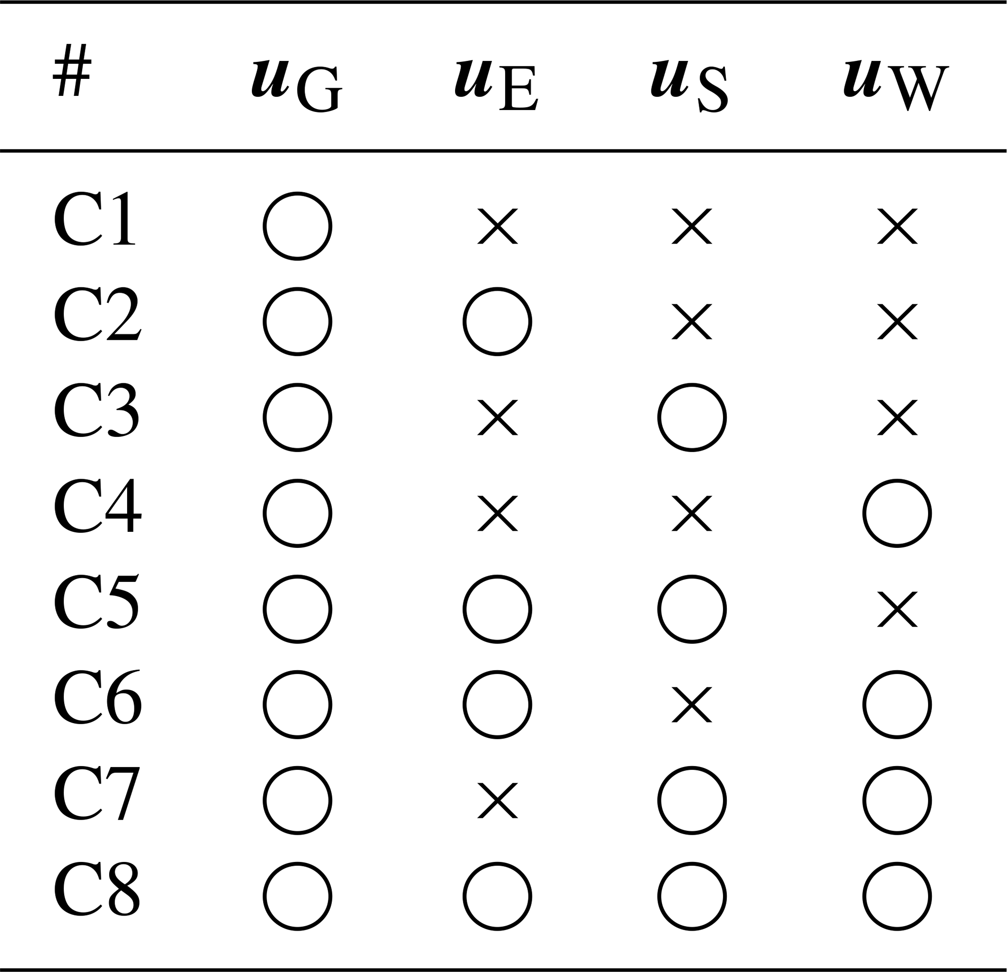
Two sets of PTM simulations were conducted using the eight forcing combinations described in Table 1: PTM-DX, representing the undrogued DX drifters, and PTM-DO, representing the drogued DO drifters. For PTM-DX, near-surface forcings were used. Specifically, the Stokes drift was sampled from the shallowest available subsurface level of the wave-model output, approximately $z=-\mathrm{0.1}$ m, while the Ekman current was evaluated near the surface. This depth is more representative of the effective submerged depth of the DX drifter than a strict air–sea interface value, because most of the cylindrical body was submerged within the upper 0.25–0.27 m of the water column. For PTM-DO, the Stokes drift and Ekman current were sampled at an effective depth of $z=-\mathrm{1.5}$ m. This depth was estimated from the area-weighted hydrodynamic centroid of the submerged cylindrical body and drogue. The submerged cylindrical body had a projected area of approximately $\mathrm{0.09}\times \mathrm{0.26}=\mathrm{0.0234}$ m², with its centroid near 0.13 m depth, whereas the effective projected area of one 0.30×0.30 m drogue plate was 0.09 m², centered near 2.0 m depth. The resulting area-weighted centroid was approximately 1.6 m below the sea surface. Thus, $z=-\mathrm{1.5}$ m provides a reasonable effective sampling depth for representing the combined hydrodynamic response of the surface float and the submerged drogue. To evaluate the optimal forcing combination, one particle was released from each drifter's initial location, and each simulation was run for 79 d, corresponding to the longest observed drifter track.

Table 1 Forcing-component combinations used in the particle tracking model (PTM) simulations. The columns indicate the four velocity components: u_G (geostrophic current), u_E (Ekman current), u_S (Stokes drift), and u_W (ru₁₀). Circles (◦) indicate that the component was included, whereas crosses (×) indicate that it was excluded. C1 represents the geostrophic-only reference case; C2–C4 represent two-component forcing cases; C5–C7 represent three-component forcing cases; and C8 represents the four-component forcing case. These combinations were used to simulate particle trajectories for comparison with the observed DX (undrogued) and DO (drogued) drifters. For PTM-DX, near-surface forcing components were used. For PTM-DO, the Ekman current and Stokes drift were sampled at an effective depth of 1.5 m to represent the deeper hydrodynamic response of the drogued drifters.

2.4 Evaluation of the particle trajectory

The particle trajectories calculated from the PTM were compared with observed drifter trajectories to determine the optimal combination of forcing components representing near-surface currents. The Mean Absolute Error (MAE), and the Normalized Cumulative Lagrangian separation (NCLS) (Kim et al., 2023) were used as metric to quantify the difference between particle and drifter trajectories. The equation for the MAE is given by,

$$\begin{array}{}\text{(7)}& \mathrm{MAE}={\displaystyle \frac{\mathrm{1}}{N}}\sum _{i=\mathrm{1}}^N(\left|\mathrm{\Delta }\mathrm{Lon}\right|+\left|\mathrm{\Delta }\mathrm{Lat}\right|)\end{array}$$

where ΔLon and ΔLat are the differences between longitude and latitude of the observed and predicted trajectories. N is the number of the dataset (Kim et al., 2023). The longitude and latitude differences were first converted into physical distances (km) before calculating the MAE. Lower MAE values indicate more precise forecasts and better overall performance.

The NCLS is defined as the cumulative summation of the separation distance between the particle and drifter trajectories, weighted by the length of the drifter trajectories accumulated in time, as follow:

$$\begin{array}{}\text{(8)}& \mathrm{NCLS}=\left\{\begin{array}{ll}\mathrm{1}-\frac{s}{n}& (s\le n)\\ \mathrm{0}& (s>n)\end{array}\right.,\end{array}$$

where s ($=\frac{{\sum }_{i=\mathrm{1}}^N{D}_i}{{\sum }_{i=\mathrm{1}}^N{L}_{\mathrm{o},i}}$) denotes the normalized cumulative separation distance and n is a dimensionless value representing the allowed threshold. This study adopted a value of n=1, consistent with the approach used by Kim et al. (2023), Liu and Weisberg (2011) and Liu et al. (2014). D_i is the separation distance between drifter and particle trajectories at time step i, L_o,i is the cumulative length of the observed trajectories at time step i. Thus, MAE and NCLS are the dimensional and nondimensional metrics, respectively, that measure the cumulative error between the simulated particle and observed drifter trajectories. NCLS values closer to 1 (with a range of 0 to 1) indicate a more accurate simulation.

2.5 Lagrangian diagnostics

The dispersion of observed drifters and simulated particles was quantified using two pair-based metrics: the relative dispersion (R²(t)) and the Finite-Scale Lyapunov Exponent (FSLE). The relative dispersion indicates the growth in size of the drifter cluster relative to its center of mass as given by

$$\begin{array}{}\text{(9)}& R^{\mathrm{2}}\left(t\right)={\displaystyle \frac{\mathrm{1}}{N}}\sum _{i=\mathrm{1}}^N{\left[{\mathit{x}}_i\left(t\right)-{\mathit{x}}_{\mathrm{cm}}\left(t\right)\right]}^{\mathrm{2}},\end{array}$$

where N is the number of drifters, x_i(t) is the position vector of the ith drifter at time t, and x_cm(t) is the position vector of the center of mass of the drifter cluster at time t (LaCasce, 2008). For the relative-dispersion analysis, only drifter pairs with an initial separation distance of less than 200 m were retained. The corresponding dispersion coefficient (K) was estimated as

$$\begin{array}{}\text{(10)}& K={\displaystyle \frac{\mathrm{1}}{\mathrm{4}}}{\displaystyle \frac{{\mathit{\sigma }}_{\mathrm{r}}^{\mathrm{2}}}{t}},\end{array}$$

where ${\mathit{\sigma }}_{\mathrm{r}}^{\mathrm{2}}$ represents the horizontal radial variance of the drifter or particle distribution. It is calculated from the mean squared distance of the particles from the center of mass of the cloud and can be interpreted as the spreading scale of an equivalent radially symmetric distribution. Thus, ${\mathit{\sigma }}_{\mathrm{r}}^{\mathrm{2}}$ quantifies the radial spreading of the drifter or particle cloud and was used to estimate the horizontal dispersion coefficient (Okubo, 1971; LaCasce, 2008). Different scaling regimes of R²(t) with time indicate different dispersion processes e.g., R²(t)∼t for diffusive dispersion, R²(t)∼t³ for Richardson dispersion, which correspond to K∼L⁰ and $K\sim L^{\mathrm{4}/\mathrm{3}}$, respectively, where L is 3σ_r represents the size of the particle cluster.

In addition to relative dispersion, the FSLE was also calculated to characterize the dispersion process. The FSLE (λ), measures the average rate of separation of initially nearby particles over a finite distance. It is calculated by tracking pairs of particles and measuring the time it takes for their separation to grow from an initial separation distance, δ₀, to a final separation distance, δ_f:

$$\begin{array}{}\text{(11)}& \mathit{\lambda }={\displaystyle \frac{\mathrm{1}}{\langle \mathrm{\Delta }t\rangle }}\ln \left({\displaystyle \frac{{\mathit{\delta }}_{\mathrm{f}}}{{\mathit{\delta }}_{\mathrm{0}}}}\right),\end{array}$$

where Δt is the time required for the pair separation to grow from the initial separation scale δ₀ to the final separation scale δ_f, and the angle brackets 〈 〉 denote an average over all particle pairs (Aurell et al., 1996). In this study, the final separation distance was defined as δ_f=2δ₀. Therefore, the FSLE plotted as a function of separation distance δ represents the growth rate from δ₀=δ to δ_f=2δ. A larger FSLE value indicates a faster rate of separation and thus stronger strain rate. Like the relative dispersion, difference scaling regimes of FSLE with respect to separation distance δ reveal different dispersion processes: $\mathit{\lambda }\sim {\mathit{\delta }}^{-\mathrm{1}}$ for ballistic dispersion (R²(t)∼t²), $\mathit{\lambda }\sim {\mathit{\delta }}^{-\mathrm{1}/\mathrm{2}}$ for Richardson-like dispersion (R²(t)∼t³), and $\mathit{\lambda }\sim {\mathit{\delta }}^{-\mathrm{2}}$ for diffusive dispersion (R²(t)∼t) (McWilliams, 2016).

The finite-time Lyapunov exponent (FTLE) was used to identify Lagrangian transport structures in the velocity fields. The FTLE quantifies the finite-time separation rate of initially neighboring particles and is defined as

$$\begin{array}{}\text{(12)}& {\mathit{\sigma }}_T\left({\mathit{x}}_{\mathrm{0}}\right)={\displaystyle \frac{\mathrm{1}}{\left|T\right|}}\ln \sqrt{{\mathit{\lambda }}_{\max }\left(\mathbf{C}\right)},\end{array}$$

where x₀ is the initial particle position vector, T is the integration time, C is the Cauchy–Green strain tensor, and λ_max(C) is the largest eigenvalue (Haller and Yuan, 2000; Shadden et al., 2005; Haller, 2015). The Cauchy–Green strain tensor is given by

$$\begin{array}{}\text{(13)}& \mathbf{C}={\left[\mathrm{\nabla }{F}_{t_{\mathrm{0}}}^{t_{\mathrm{0}}+T}\left({\mathit{x}}_{\mathrm{0}}\right)\right]}^T\left[\mathrm{\nabla }{F}_{t_{\mathrm{0}}}^{t_{\mathrm{0}}+T}\left({\mathit{x}}_{\mathrm{0}}\right)\right],\end{array}$$

where $F_{t_{\mathrm{0}}}^{t_{\mathrm{0}}+T}\left({\mathit{x}}_{\mathrm{0}}\right)$ is the flow map that gives the particle position at time t₀+T from the initial position x₀ at time t₀. Ridges of the FTLE field have been widely used as indicators of Lagrangian coherent structures that organize material transport and mixing (Haller and Yuan, 2000; Shadden et al., 2005; Haller, 2015). In particular, repelling FTLE ridges are associated with material lines from which neighboring particles separate, whereas attracting FTLE ridges are associated with material lines toward which neighboring particles converge (Haller, 2001; Shadden et al., 2005). A finite-time hyperbolic region can be identified near the intersection of attracting and repelling ridges, where particles converge toward the attracting manifold and subsequently diverge along the repelling manifold (Haller and Yuan, 2000; Shadden et al., 2005). Such a saddle-type Lagrangian structure represents a dynamically important transport barrier and can explain the bifurcation of drifter trajectories.

3 Results

3.1 Drifter trajectory

All analyzed drifters deployed near the Korean coast, except those that stopped transmitting before beaching, ultimately reached the Japanese mainland or nearby islands within 13–68 d, while eight drifters stopped before beaching after 6–79 d (Table 2). Figure 2a shows the trajectories and final positions of the undrogued DX and drogued DO drifters. Within a few days after deployment, the drifters began diverging into two distinct pathways. One group, comprising 60 % of the DO drifters and 27 % of the DX drifters, moved northward along the eastern coast of Korea, likely influenced by the strong East Korea Warm Current (EKWC). The other group, consisting of 40 % of the DO drifters and 73 % of the DX drifters, drifted eastward toward the Japanese coast, primarily driven by prevailing westerly winds. The drifter bifurcation was further examined using FTLE structures derived from the geostrophic velocity field (Fig. 2b). The signed FTLE field shows that the bifurcation occurred near 130° E, 37.4° N, where attracting and repelling FTLE ridges are closely organized. In this representation, red ridges indicate attracting Lagrangian structures, whereas blue ridges indicate repelling Lagrangian structures (Fig. 2b). The observed drifters approached this region from the south to southwest and then separated into two branches, one moving northwestward and the other moving southeastward. This behavior is consistent with a finite-time hyperbolic-type bifurcation region, where particles converge toward an attracting manifold and subsequently diverge along a repelling manifold. This region was located near 130° E, 37.4° N, corresponding to the observed divergence of the drifter trajectories. The mean speeds of the DO and DX drifters were calculated as 0.28 and 0.31 m s⁻¹, respectively.

Table 2 Summary of the final fate and drifting duration of observed drifters. The table lists the number and percentage of drifters in each fate category, the corresponding drifting–duration range, and the final fate.

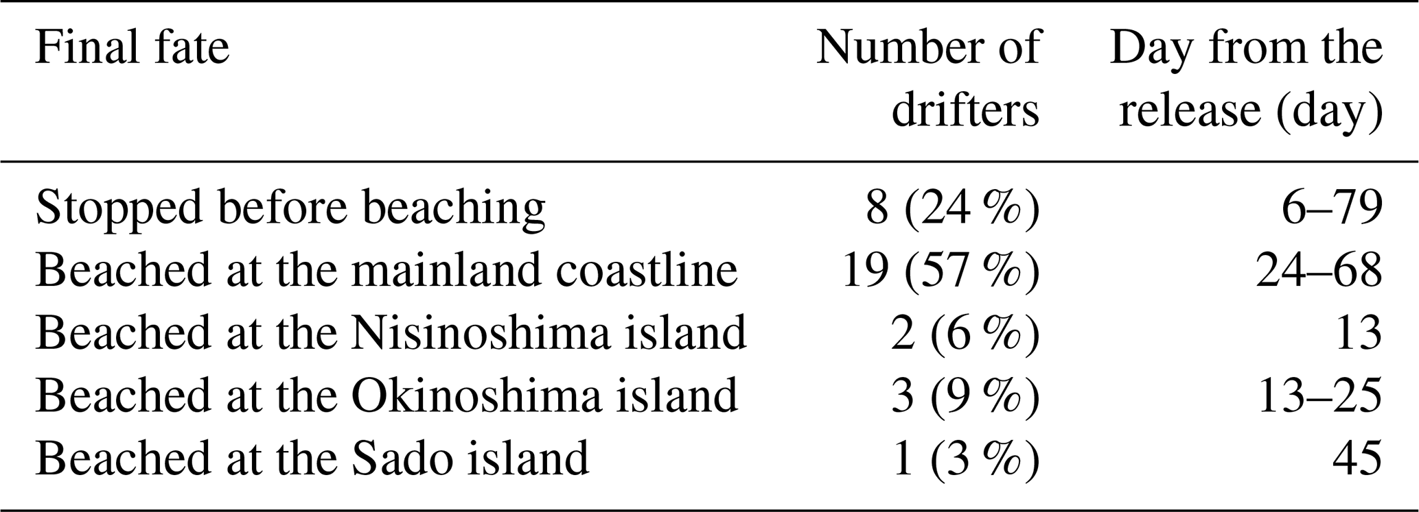
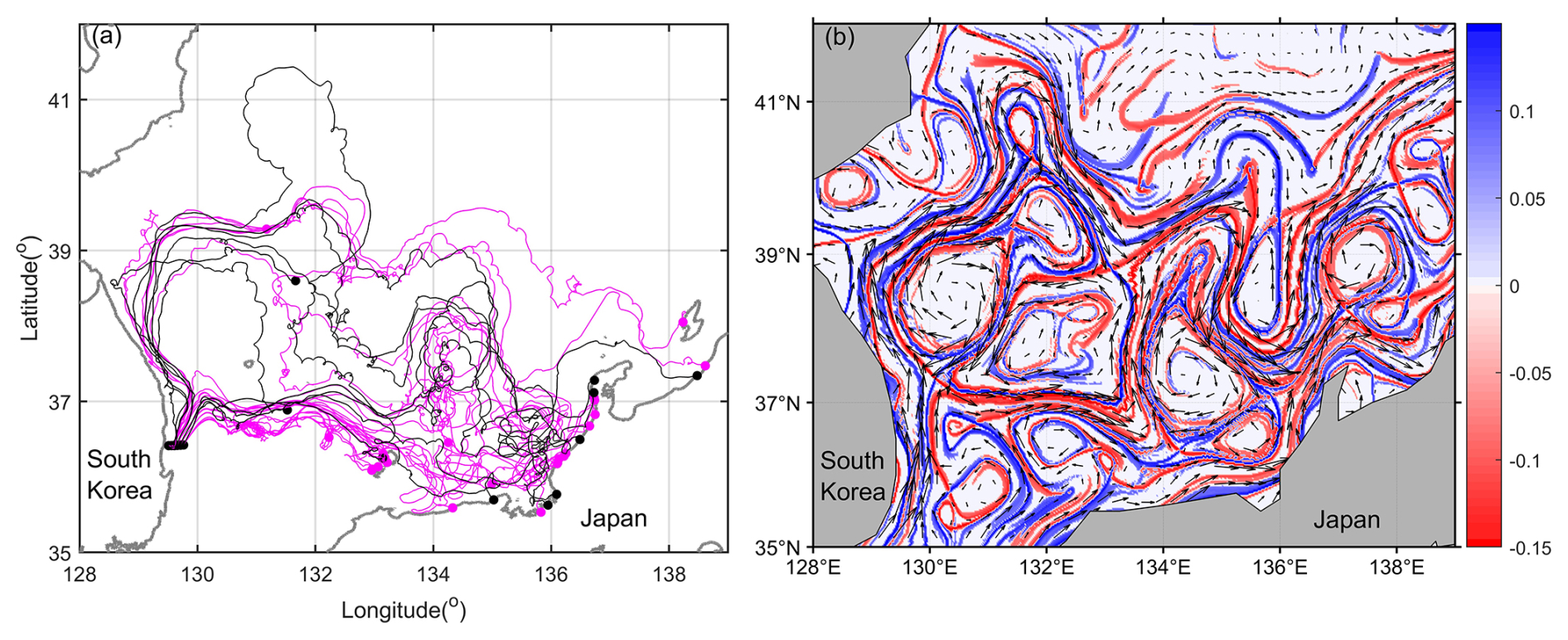
Figure 2 (a) Observed trajectories of undrogued DX drifters (black lines) and drogued DO drifters (magenta lines). Thick black lines indicate the initial deployment locations, and filled circles denote the final positions of drifters that remained at sea. (b) Signed Finite-time Lyapunov exponent (FTLE) field computed from the geostrophic velocity averaged over the first week after drifter release. Black arrows indicate the geostrophic velocity vectors. In the signed FTLE representation, blue and red ridges indicate repelling and attracting Lagrangian structures, respectively.

3.2 Drifter dispersion

The time evolution of the relative dispersion, D²(t) (Eq. 9), and the dispersion coefficient, K(L) (Eq. 10), for the drifters is illustrated in Fig. 3. At very early times (t<0.3 d) and small length scales (L<1 km), the drifter cluster exhibited diffusive dispersion (D²∼t¹). Beyond this initial stage, Richardson dispersion (D²∼t³, or equivalently, $K^{\mathrm{2}}\sim L^{\mathrm{4}/\mathrm{3}}$), was evident in the range of approximately 0.3 to 30 d, corresponding to length scales from L=1 to 100 km. During $\mathrm{0}<t<\mathrm{3}$ (or L<60 km), the DO drifters showed slightly greater dispersion than DX drifters, which was possibility attributed to the different passages determined at the hyperbolic region. The majority of DO drifters followed passage along the EKWC near the Korean coastline, where horizontal shear in the coastal current can enhance the dispersion. In contrast, the majority of DX drifters moved offshore, where the transport was dominated by spatially uniform wind in a narrow directional range, resulting in relatively weaker dispersion during the time. However, after approximately 3 d, as the DX drifters moved farther offshore, interactions with mesoscale eddies in the westerly downwind regions enhanced their dispersion, leading to super-Richardson behavior and causing their relative dispersion to exceed that of the DO drifters.

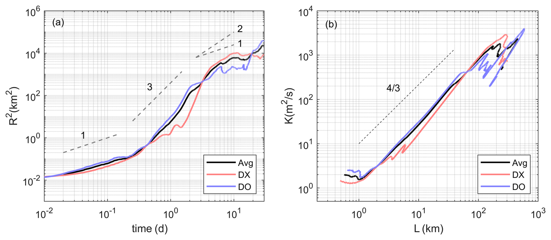
Figure 3 Relative dispersion (R(t)²) (a) and dispersion coefficient (K(L)) (b) of the observed drifters. Panel (a) shows the time evolution of relative dispersion (R(t)²), and panel (b) shows the dispersion coefficient (K(L)) as a function of length scale. The red line represents the undrogued (DX) drifters, the blue line represents the drogued (DO) drifters, and the black line indicates the average dispersion of all drifters (both DX and DO).

The estimated dispersion coefficients for all drifters were approximately 1, 20, and 1000 m² s⁻¹ at scales of 1, 10, and 100 km, respectively, eventually saturating around 2000 m² s⁻¹ in the EJS. The dispersion coefficient at the early stage was comparable to previous dye and drifter experiments in various waters, including coastal regions, inland waters, and open oceans (Okubo, 1971; Choi et al., 2020; Kim et al., 2024). For scales of 1–100 km, the growth in dispersion followed trends observed in open oceans, and the coefficient saturated when the length scale of the drifter cloud reached approximately 1/10 of the basin scale of the EJS (∼2000 km).

The FSLE values and trends for both DX and DO drifters were generally similar, but the FSLE values for DO drifters were slightly higher, particularly at very early times at spatial scales on the order of 10 m and between 0.5 and 50 km. This pattern aligns with the dispersion coefficient K shown in Fig. 3b, where K is also larger for DO drifters over these scales. The difference in FSLE between DO and DX drifters is likely due to their distinct pathways delineated by the hyperbolic-type bifurcation region, consistent with observations from the relative dispersion analysis. The FSLE curves reveal distinct dynamical regimes across spatial scales. In the small-scale regime (δ<0.5 km), DX drifters exhibit a slope close to −1, indicative of ballistic dispersion, possibly associated with well-aligned wind-induced transport. In the submeso- and mesoscale-range (1 km < δ < 50 km), the slope for DX drifters becomes slightly gentler, and FSLE values remain lower than those of DO drifters. For DO drifters, the FSLE initially shows a steep slope near −2 at small scales (δ<0.5 km), characteristic of a diffusive regime, then transitions to a slope of approximately $-\mathrm{1}/\mathrm{2}$ to $-\mathrm{2}/\mathrm{3}$, reflecting Richardson-like dispersion (Fig. 4). This behavior is consistent with the influence of coastal currents and mesoscale eddy interactions in the region. At larger scales (beyond ∼150 km), both DX and DO drifters show a steepening of FSLE values again, corresponding to the scale of mesoscale eddies in the EJS.

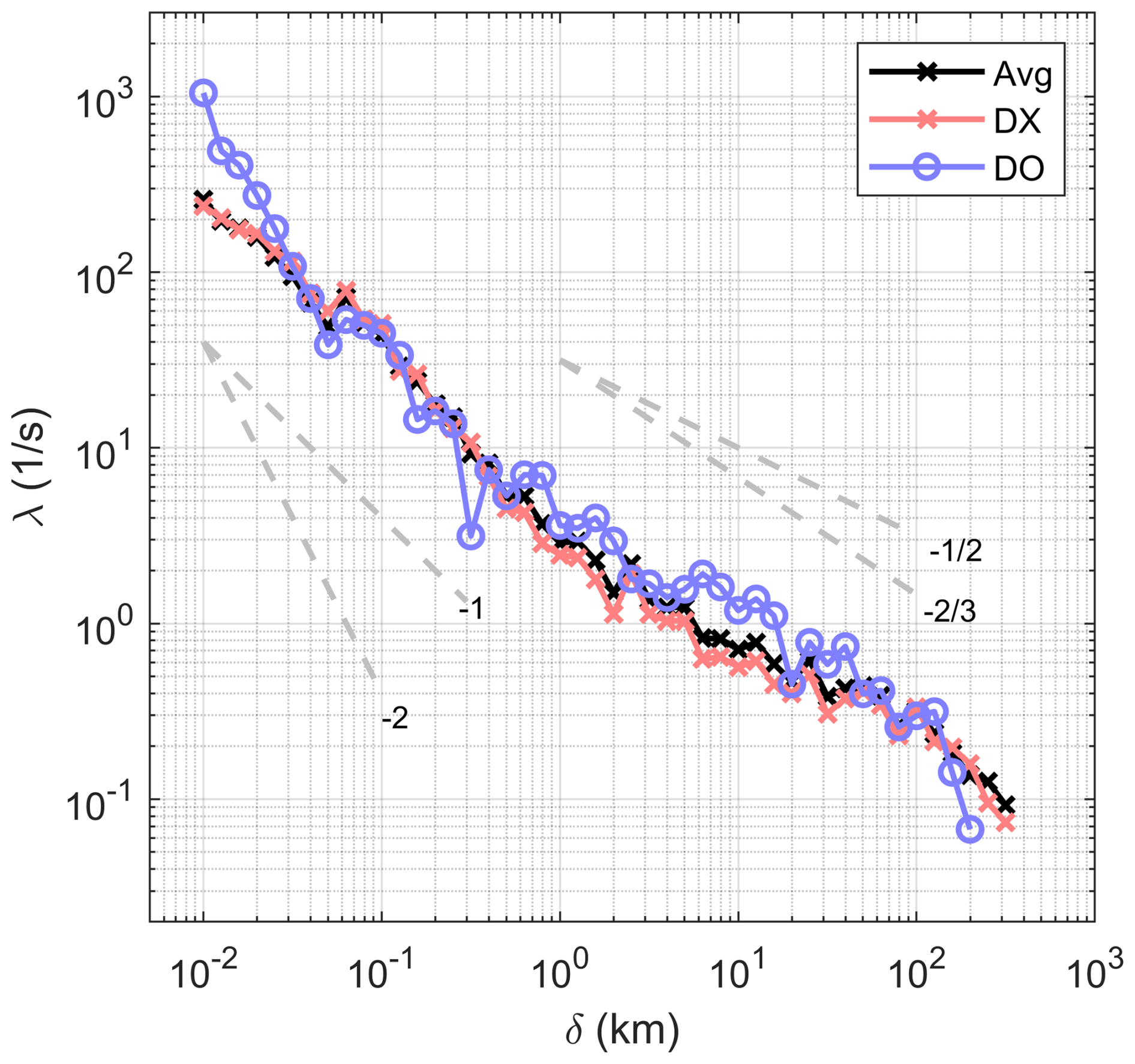
Figure 4 Finite-Size Lyapunov Exponent (FSLE), λ, as a function of separation distance, δ, for the observed drifters. The black line represents the average of all drifters, the red line represents the undrogued (DX) drifters, and the blue line represents the drogued (DO) drifters. The dashed gray lines indicate reference slopes of −2, −1, $-\mathrm{1}/\mathrm{2}$, and $-\mathrm{2}/\mathrm{3}$.

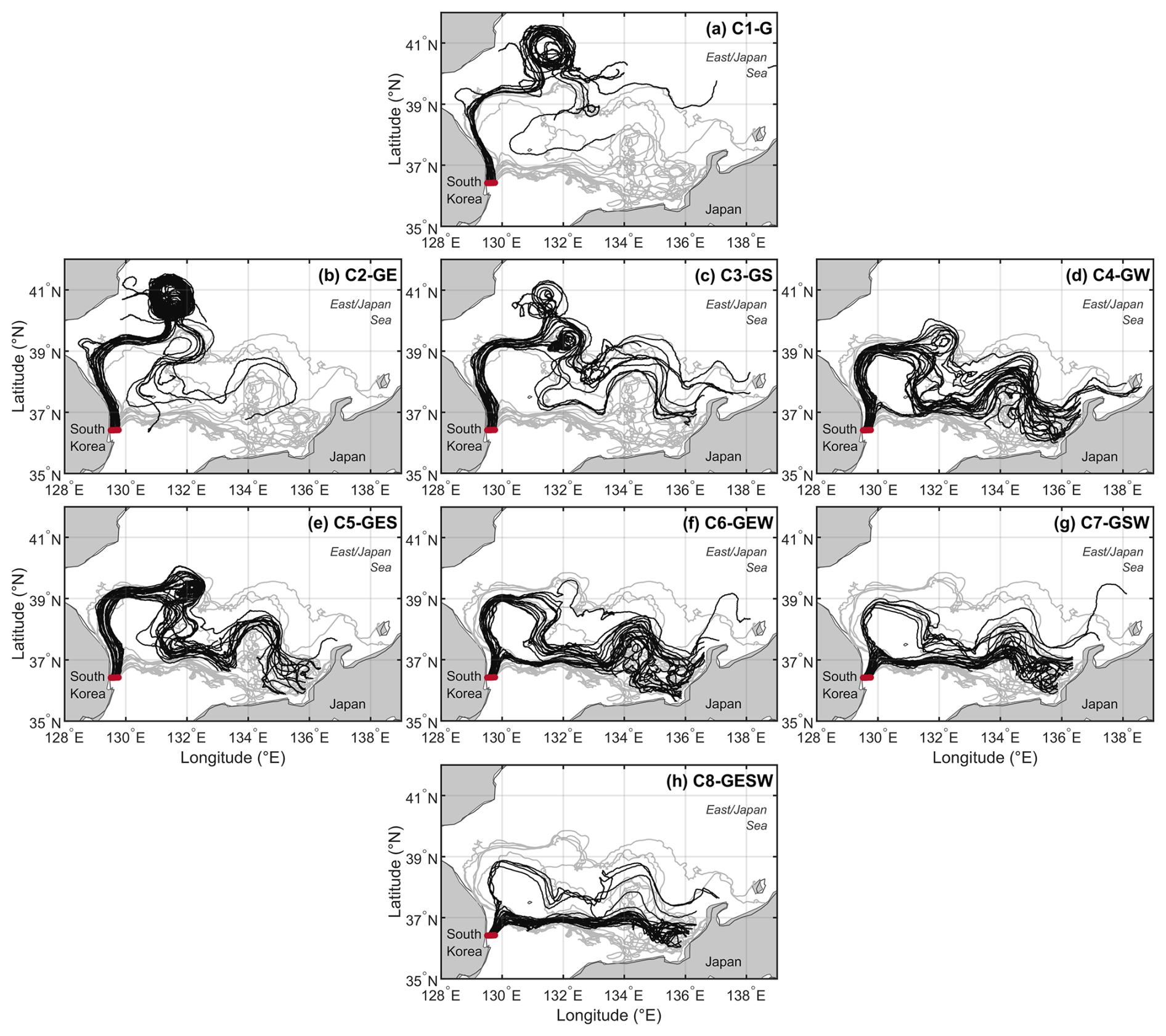
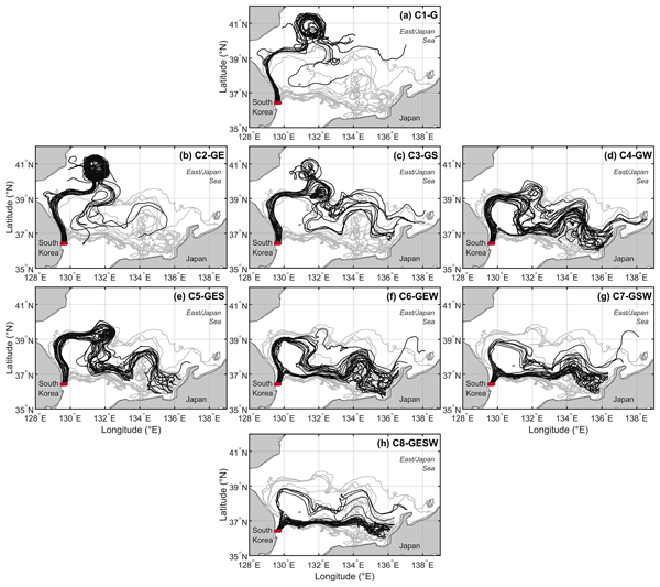
Figure 5 Observed trajectories of undrogued DX drifters (gray) and simulated PTM-DX trajectories (black) over the 79 d simulation period for forcing combinations C1–C8 listed in Table 1. Red markers indicate the initial release locations. All panels use the same geographic domain, coordinate units, and labels for South Korea, Japan, and the East/Japan Sea. Panels (a)–(h) correspond to C1–C8 and are arranged by the number of forcing components: C1; C2–C4; C5–C7; and C8. G, E, S, and W denote geostrophic current, Ekman current, Stokes drift, and windage, respectively.

3.3 Particle trajectory

The performance of the forcing combinations listed in Table 1 was evaluated by qualitatively comparing the observed drifter trajectories with simulated particle trajectories at two different depths: DX drifters were compared with PTM-DX particles driven by surface forcings (Fig. 5), while DO drifters were compared with PTM-DO particles driven by subsurface forcings at 1.5 m depth (Fig. 6). For the PTM-DX particles, increasing the number of forcing components improved the model's ability to replicate the bifurcation of drifter trajectories at the hyperbolic region, particularly when windage was included (Fig. 5f–h). When simulations were driven solely by geostrophic currents (Fig. 5a), all particles drifted predominantly northward along the EKWC, ultimately accumulating in a mesoscale eddy centered near 132° E, 41° N. The addition of Ekman currents (Fig. 5b) did not result in significant differences. However, including Stokes drift (Fig. 5c) reduced the residence time of particles within the eddy and redirected them toward the Japanese coast. In all simulations without windage, particles remained confined along the EKWC, whereas simulations incorporating windage produced more realistic trajectories that aligned with observed DX drifter paths, which split into both coastal and offshore passages. For PTM-DO particles (Fig. 6), all forcing combinations resulted in transport along the EKWC. The variation among trajectories was less pronounced than for PTM-DX, indicating a stronger influence of the coastal current. Although none of the PTM-DO simulations captured the bifurcation at the hyperbolic-type bifurcation region, the simulation including all four components, geostrophic currents, Ekman currents, Stokes drift, and windage (Fig. 6h), most closely reproduced the observed DO drifter trajectories.

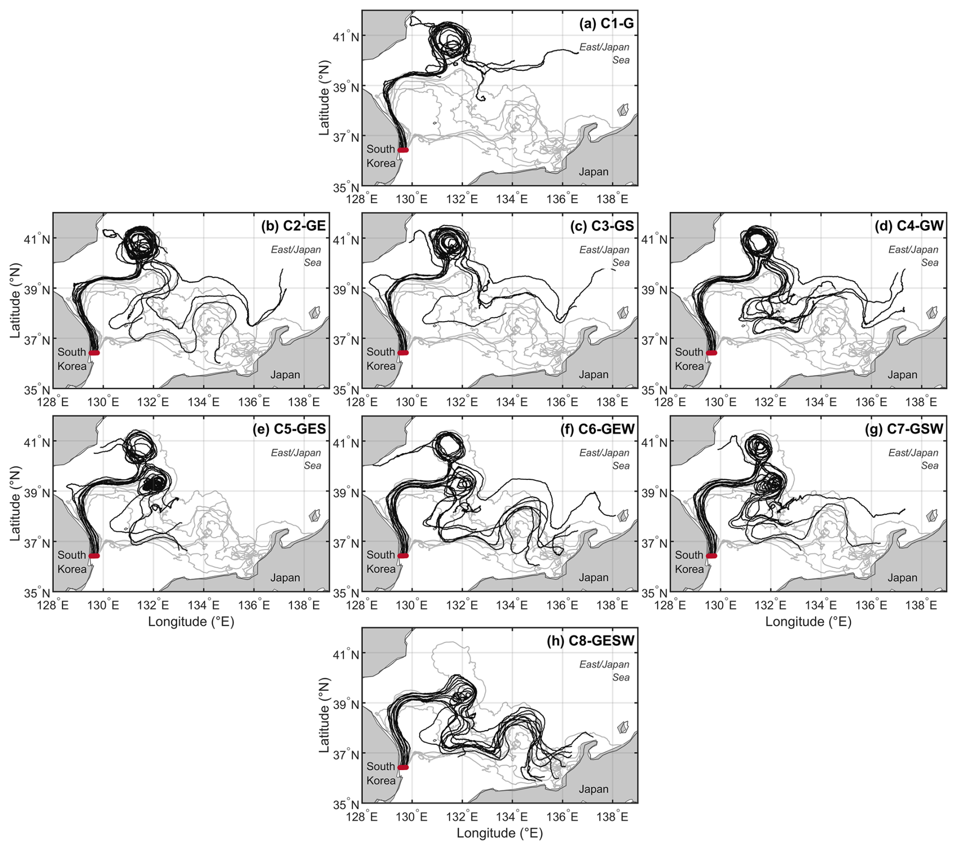
Figure 6 Observed trajectories of drogued DO drifters (gray) and simulated PTM-DO trajectories (black) over the 79 d simulation period for forcing combinations C1–C8 listed in Table 1. For PTM-DO, the Ekman current and Stokes drift were evaluated at the effective depth of 1.5 m. Red markers indicate the initial release locations. All panels use the same geographic domain, coordinate units, and labels for South Korea, Japan, and the East/Japan Sea. Panels (a)–(h) correspond to C1–C8 and are arranged by the number of forcing components: C1; C2–C4; C5–C7; and C8. G, E, S, and W denote geostrophic current, Ekman current, Stokes drift, and windage, respectively.

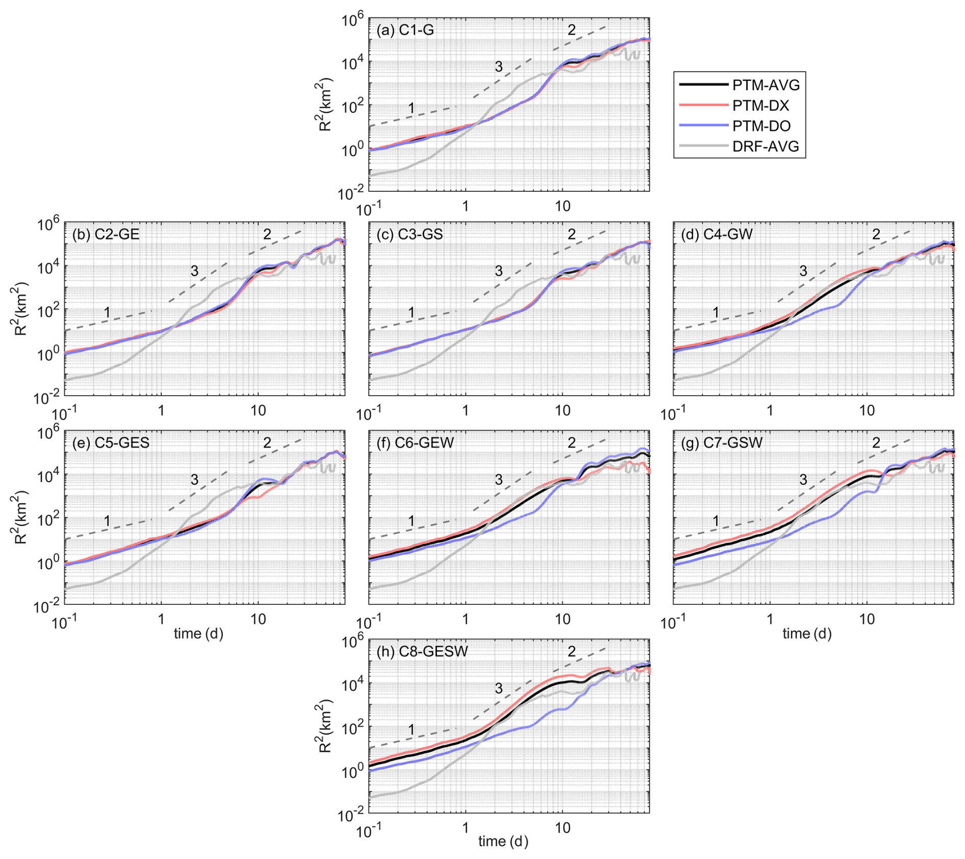
Figure 7 Relative dispersion (R²(t)) of particles simulated with different forcing combinations (C1–C8) as described in Table 1, shown alongside observed drifter dispersion. Panels are arranged in the same order as in Figs. 5 and 6. Red and blue lines represent the relative dispersions for PTM-DX and PTM-DO simulations, respectively, and the gray line represents the average relative dispersion of the observed drifters for comparison. G, E, S, and W indicate geostrophic current, Ekman current, Stokes drift, and windage forcings, respectively.

3.4 Particle dispersion

Figure 7 presents the time evolution of relative dispersion, D²(t), for PTM-DX and PTM-DO particles under the eight forcing combinations (C1–C8). Overall, the two PTM sets exhibited comparable dispersion magnitudes and slopes; however, notable differences arose when windage was included. In cases where windage was applied (Fig. 7d and f–h), PTM-DX particles exhibited greater dispersion than PTM-DO particles, contrary to the drifter observations, which showed that DO drifters experienced higher dispersion, particularly at mesoscale distances. This discrepancy stemmed from the model's failure to reproduce the bifurcation at the hyperbolic-type bifurcation region. In the observations, both DX and DO drifters split between an offshore path and the EKWC path, albeit with different proportions: more DX drifters followed the offshore route, while more DO drifters remained along the EKWC, where coastal shear enhanced dispersion. In contrast, the simulations confined all PTM-DO particles to the EKWC path, while PTM-DX particles were distributed between both paths. Since particles restricted to the EKWC path experience weaker dispersion compared to those traversing both the EKWC and offshore routes, the PTM-DO simulations underestimated dispersion relative to PTM-DX, opposite to the pattern observed in the drifter data. Both particles and drifters exhibited a diffusive phase during the early stages; however, this phase persisted only briefly for the drifters (t<0.3 d), while it extended significantly longer for the particles, up to approximately 2 d, until the average pairwise separation distance reached approximately 25 km, corresponding to the grid spacing of the velocity field used in the PTM calculations. As a result, the effective diffusivity of particle pairs separated by less than 25 km was substantially higher than that observed in the drifter data. This discrepancy arises from the Smagorinsky scheme, which applies a constant diffusion coefficient within each 25 km grid cell, leading to artificially enhanced diffusion at very early times in all PTM simulations. The domain-averaged horizontal diffusion coefficient during the drifter observation period (November 2021 to February 2022), computed using the Smagorinsky parameterization, was approximately 87.3 m² s⁻¹. This value is consistent with the empirical, scale-dependent horizontal diffusivity described by Okubo (83.7 m² s⁻¹), given by K=0.0103L^1.15, where K is in cm² s⁻¹ and L is the spatial scale in cm. In this context, L is taken as 3σ_r, or equivalently 3Δx, with Δx=25 km representing the grid spacing of the velocity field used in the PTM simulations.

The FSLE (λ) for the particle simulations (C1–C8) showed only minor differences among the various forcing combinations (Fig. 8). FSLE values from simulated particles and observed drifters became comparable at spatial scales greater than approximately 25 km, which aligns closely with the spatial grid size used for the current data in the simulations. At scales smaller than approximately 25 km, the FSLEs of the simulated particles were roughly three times greater than those observed from real drifters. This disparity at smaller scales occurs because particles in simulations are initially confined within grid cells, influenced significantly by numerical diffusion inherent in the Smagorinsky scheme. At these early times and small scales, the FSLE slopes for the drifters and particles are approximately −1, indicative of a ballistic dispersion regime. At intermediate spatial scales between about 25 and 200 km, the FSLE curves for the simulated particles exhibit a slope closer to $-\mathrm{1}/\mathrm{2}$, signifying a local dispersion regime. Beyond roughly 200 km, the FSLE slopes steepen, approaching a slope of about $-\mathrm{5}/\mathrm{4}$, particularly evident in simulations where many particles eventually reach the coastline.

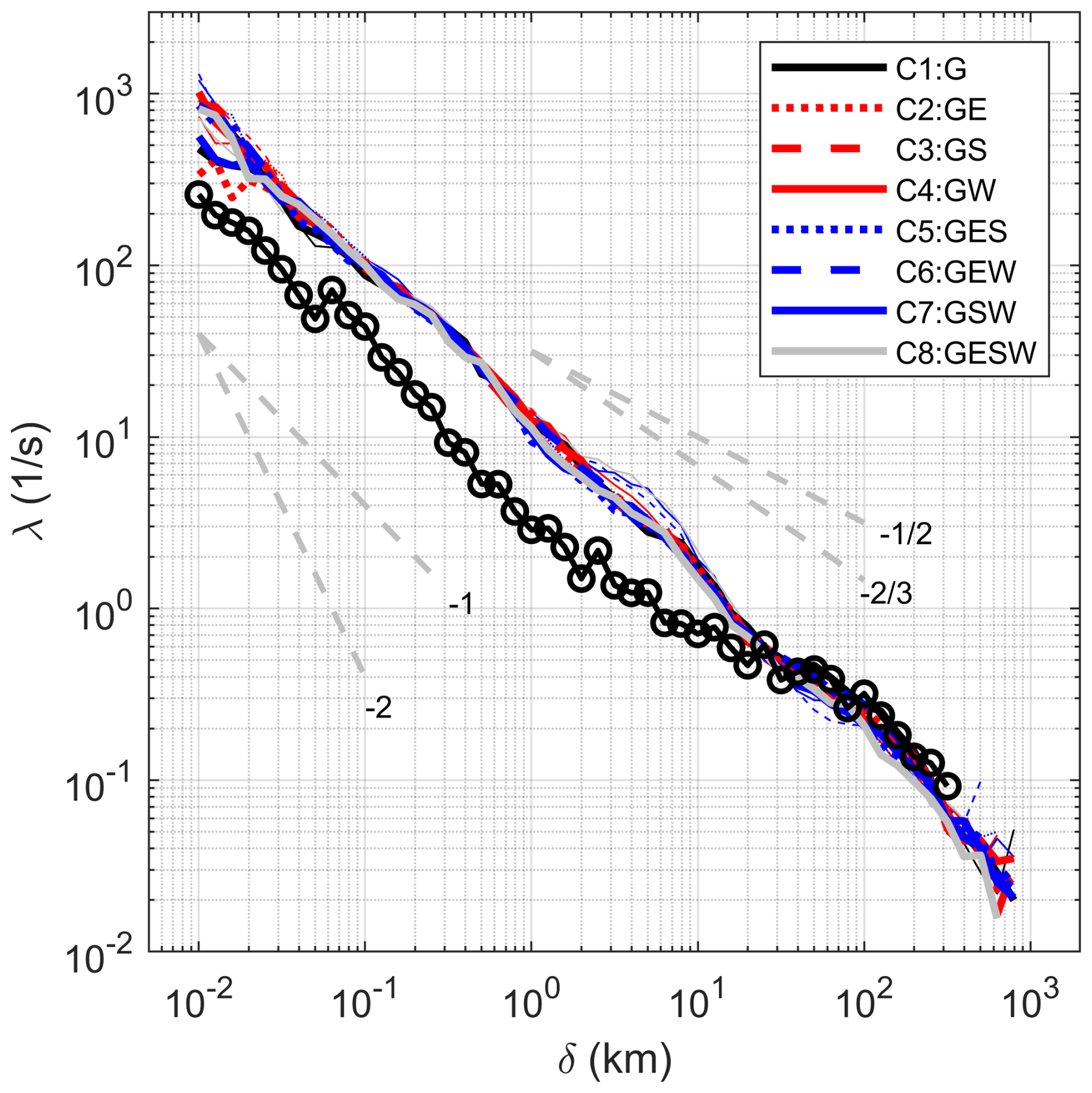
Figure 8 Finite-Size Lyapunov Exponent (FSLE), λ, as a function of separation distance, δ, for the simulated particles and observed drifters. The black line with circles represents the FSLE averaged for all observed drifters. Other colored lines show FSLEs for simulated particles from different forcing combinations (C1–C8, as listed in Table 1). Thinner lines indicate PTM-DX simulations, and thicker lines indicate PTM-DO simulations. The variation in FSLE values between different forcing combinations and between PTM-DX and PTM-DO were small.

3.5 Data-driven optimal forcing combinations

The performance of the different data-driven forcing combinations was evaluated using the mean absolute error (MAE; Eq. 7) and the normalized cumulative Lagrangian separation skill score (NCLS; Eq. 8). The MAE values at selected time steps are summarized in Table 3, whereas the NCLS results are presented as temporal variations in Fig. 9 rather than in a separate table. Together, these two metrics were used to evaluate both the magnitude of trajectory error and the temporal consistency of model skill. The values in parentheses in Table 3 indicate the ratio of each MAE to the lowest MAE at the corresponding time step; therefore, values closer to 1 indicate better relative performance.

Table 3 MAE values for undrogued particles (PTM-DX) and drogued particles (PTM-DO) under 467 different forcing combinations (C1–C8) over time. Lower MAE values indicate better model 468 performance. Bolded values represent the lowest MAE for each time step. Values in 469 parentheses show the ratio of each MAE to the lowest MAE for that time step, a ratio closer to 470 1 denotes better relative performance.

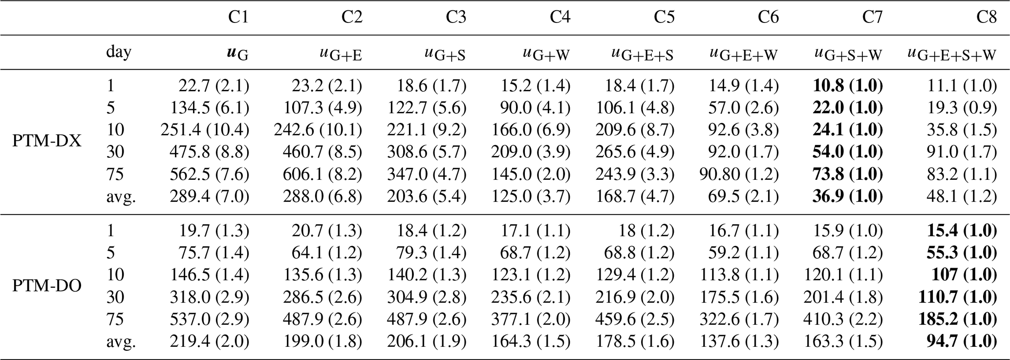
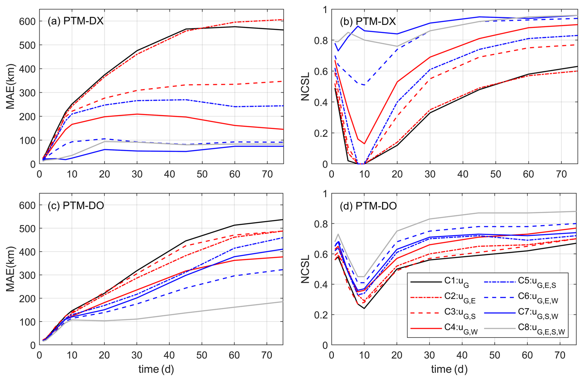
Figure 9 Temporal evolution of MAE for PTM-DX simulations (a) and PTM-DO simulations (c), and temporal evolution of NCLS for PTM-DX simulations (b) and PTM-DO simulations (d) for different forcing combinations (C1–C8, as listed in Table 1).

For PTM-DX, the simulation using only the geostrophic current (C1) showed the poorest overall performance, with an average MAE of 289.4 km. Adding the Ekman current to the geostrophic current (C2) did not improve the trajectory prediction, indicating that the Ekman component alone was insufficient to reproduce the observed DX drifter pathways. In contrast, the addition of windage substantially improved model performance. Among the two-component combinations, C4, which included geostrophic current and windage, reduced the average MAE to 125.0 km. This improvement suggests that direct wind forcing played an important role in the motion of the undrogued DX drifters.

Among the three-component combinations for PTM-DX, C7, which combined geostrophic current, Stokes drift, and windage, provided the best overall performance. C7 produced the lowest average MAE of 36.9 km and showed the highest or near-highest skill over most of the simulation period. Although C8, which included all four forcing components, showed slightly better performance at day 5, its average MAE was larger than that of C7. This result indicates that adding the Ekman current to the DX simulation did not further improve the prediction and could even degrade the trajectory skill after the early separation stage. Therefore, the optimal data-driven forcing combination for PTM-DX was identified as C7, consisting of geostrophic current, Stokes drift, and windage.

To evaluate sensitivity to the windage coefficient r without treating it as a free tuning parameter, PTM-DX was repeated using r=0.005 and r=0.030 around the geometry-based value r=0.015. Complete results are provided in Tables S1 and S2 of the Supplement. Across days 5, 10, 30, and 75, the lowest average MAE was 117.3 km for C8 at r=0.005, 42.9 km for C7 at r=0.015, and 88.2 km for C4 at r=0.030. Although the optimal combination changed when windage was substantially under- or overestimated, the geometry-based coefficient produced the smallest overall error and was retained without tuning.

The temporal evolution of MAE and NCLS further supports this interpretation (Fig. 9a and b). The C1 and C2 simulations exhibited rapid error growth and eventually reached MAE values of approximately 600 km. In contrast, the simulations that included windage, particularly C6, C7, and C8, maintained substantially lower MAE values. A rapid change in MAE and NCLS occurred around day 10, corresponding to the period when the particles passed near the hyperbolic-type bifurcation region off the eastern Korean coast. In this region, small differences in the early simulated trajectories can determine whether particles follow the coastal northward pathway or the offshore eastward pathway. Thus, accurately representing the early wind-driven displacement near this bifurcation region was critical for reproducing the downstream trajectories of the DX drifters.

To further examine whether the MAE-based ranking was dominated by accumulated downstream separation after the early bifurcation, we also performed a segment-based MAE analysis for the DX simulations. The observed and simulated DX trajectories were divided into 3 d segments, and the MAE was calculated independently for each segment to evaluate short-term local trajectory skill (Table S3). This analysis showed that the full forcing case, ${\mathit{u}}_{\mathrm{G}}+{\mathit{u}}_{\mathrm{E}}+{\mathit{u}}_{\mathrm{S}}+{\mathit{u}}_{\mathrm{W}}$, produced the lowest segment-based error, with $\mathrm{MAE}=\mathrm{28.7}\pm \mathrm{3.7}$ km, followed by ${\mathit{u}}_{\mathrm{G}}+{\mathit{u}}_{\mathrm{S}}+{\mathit{u}}_{\mathrm{W}}$, with $\mathrm{MAE}=\mathrm{31.3}\pm \mathrm{8.3}$ km. Thus, while the cumulative MAE identified ${\mathit{u}}_{\mathrm{G}}+{\mathit{u}}_{\mathrm{S}}+{\mathit{u}}_{\mathrm{W}}$ as the best integrated pathway predictor for DX, the segment-based analysis indicates that ${\mathit{u}}_{\mathrm{G}}+{\mathit{u}}_{\mathrm{E}}+{\mathit{u}}_{\mathrm{S}}+{\mathit{u}}_{\mathrm{W}}$ provided the most stable short-term local trajectory skill. This confirms that the windage- and Stokes-drift-inclusive forcings were important not only for the accumulated downstream pathway, but also during the early bifurcation stage.

For PTM-DO, the differences among the forcing combinations were less pronounced than for PTM-DX, reflecting the weaker direct wind response of the drogued drifters. Nevertheless, the inclusion of additional forcing components generally improved the trajectory prediction. The geostrophic-only case (C1) produced an average MAE of 219.4 km, while C4 reduced the average MAE to 164.3 km. Among the three-component combinations, C6, which included geostrophic current, Ekman current, and windage, showed the best performance, with an average MAE of 137.6 km. This result suggests that the Ekman component was more important for the drogued DO drifters than for the undrogued DX drifters, consistent with the deeper effective sampling depth of the DO drifter.

The best overall performance for PTM-DO was obtained with C8, which included geostrophic current, Ekman current, Stokes drift, and windage. C8 produced the lowest MAE at all selected time steps and reduced the average MAE to 94.7 km. The NCLS evolution also showed that C8 consistently maintained the highest trajectory skill for the DO simulations (Fig. 9c and d). Therefore, unlike the DX case, the inclusion of all four forcing components was necessary to reproduce the observed DO drifter trajectories most accurately.

To test sensitivity to the stochastic random-walk diffusion term, the PTM simulations were repeated with 10 numerical particles (realisations) for each observed drifter initial location. Only the Gaussian random sequences were varied; the deterministic velocity fields and all other settings were unchanged. Tables S4 and S5 of the Additional Materials compare the original single-particle and 10-realisation ensemble-mean MAE values. The absolute errors changed slightly, but the forcing rankings were stable: C8 remained best for PTM-DX at day 5, C7 remained best at days 10, 30, and 75, and C8 remained best for PTM-DO at all four evaluation times. The main conclusions therefore do not depend on a single stochastic realisation.

Overall, the optimal forcing combination differed between the two drifter types. For the undrogued DX drifters, the best performance was achieved by combining geostrophic current, Stokes drift, and windage, indicating that near-surface transport was strongly controlled by wave-induced drift and direct wind forcing. For the drogued DO drifters, the full forcing combination including Ekman current was required, suggesting that the deeper drogued drifters were more strongly influenced by subsurface wind-driven shear. These results demonstrate that the optimal PTM forcing depends on the effective sampling depth and wind exposure of the drifting object, and that a single surface-current forcing configuration may not be appropriate for all types of floating debris or drifters.

4 Discussions

4.1 Comparison with model-derived velocity products

The optimized data-driven forcing combinations were further compared with simulations driven by model-derived surface velocity products. In this comparison, the GOFS analysis based on HYCOM/NCODA and the GLORYS12V1 reanalysis distributed by Copernicus Marine were used as benchmark velocity fields. These products are referred to hereafter as HYC and CMS, respectively, to remain consistent with the notation used in Table 4. The purpose of this comparison was not to repeat the full forcing-decomposition experiment conducted for the data-driven approach, because these analysis/reanalysis products already assimilate observations and provide dynamically consistent surface velocity fields that may include both geostrophic and ageostrophic wind-driven components. Instead, the model-derived velocities were used directly, and additional direct windage and Stokes drift terms were tested to examine whether these processes improved the simulated pathways of the undrogued DX drifters.

Table 4 MAE and NCLS values for PTM-DX simulations driven by model-derived surface velocity products, namely the GOFS analysis based on HYCOM/NCODA and the GLORYS12V1 reanalysis distributed by Copernicus Marine, with and without additional windage and Stokes drift. HYC denotes the GOFS/HYCOM analysis, and CMS denotes the GLORYS12V1 reanalysis product GLOBAL_MULTIYEAR_PHY_001_030. W1 and W2 denote windage terms corresponding to 1.5 % and 3.0 % of the 10 m wind speed, respectively, and ST denotes the addition of Stokes drift calculated from the wave model.

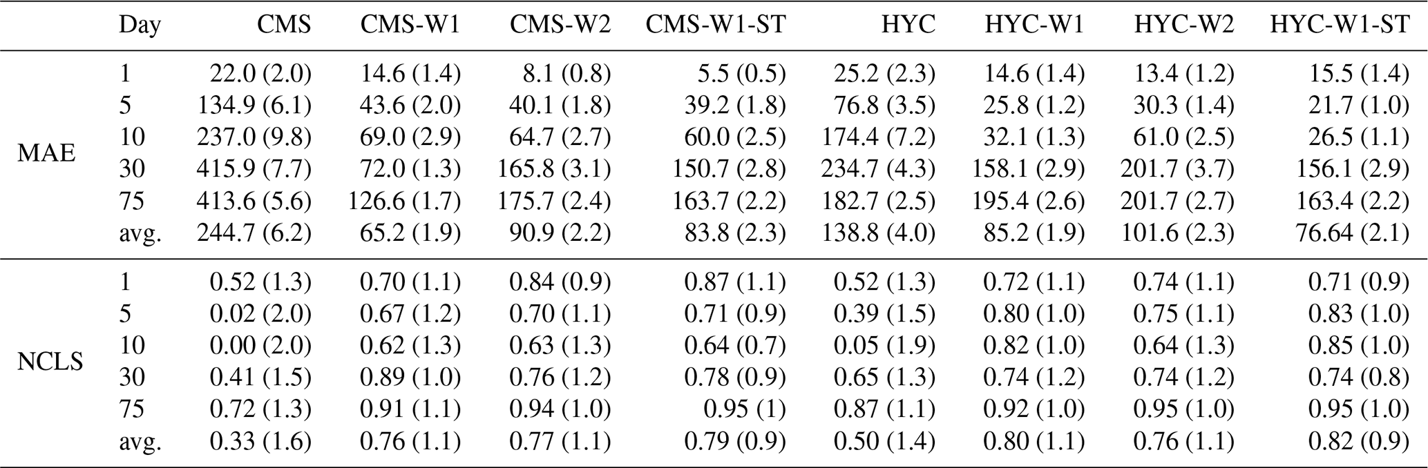
Table 4 summarizes the MAE and NCLS values for PTM-DX simulations driven by HYC and CMS, with and without additional windage and Stokes drift. In Table 4, W1 and W2 denote windage terms corresponding to 1.5 % and 3.0 % of the 10 m wind speed, respectively, while ST denotes the addition of Stokes drift calculated from the wave model. These percentages therefore refer to the windage coefficient, not to a scaling of Stokes drift. The values in parentheses are normalized by the performance of C7, which was the optimal data-driven forcing combination for PTM-DX.

The model-derived simulations generally showed poorer trajectory skill than the optimized data-driven forcing combination. Although the addition of windage and Stokes drift improved some HYC and CMS cases, the resulting MAE values remained larger and the NCLS values remained lower than those obtained with C7. This indicates that the poorer performance of HYC and CMS was not caused simply by the absence of direct windage or Stokes drift. Rather, it was related to differences in the local near-surface velocity structure during the early stage of the simulation, when small trajectory errors strongly affected the subsequent downstream pathway. The temporal resolution of the velocity products may also have contributed to these differences. The GLORYS12V1 reanalysis provides daily mean fields, whereas the wind-related components in the reconstructed forcing were derived from hourly ERA5 wind forcing. Therefore, high-frequency near-surface wind-driven variability may have been more strongly smoothed in the GLORYS-based simulation than in the reconstructed forcing fields.

To examine this mechanism, FTLE fields were computed using one-week-averaged velocity fields from the drifter release date within the same domain used for the velocity-field comparison. Figure 10 compares the FTLE structures obtained from the data-driven velocity fields and the model-derived velocity fields. The first row shows the FTLE fields for the geostrophic current alone, the data-driven combination without windage, and the data-driven combination including windage. The second and third rows show the corresponding CMS- and HYC-based cases, respectively, with and without additional windage and Stokes drift.

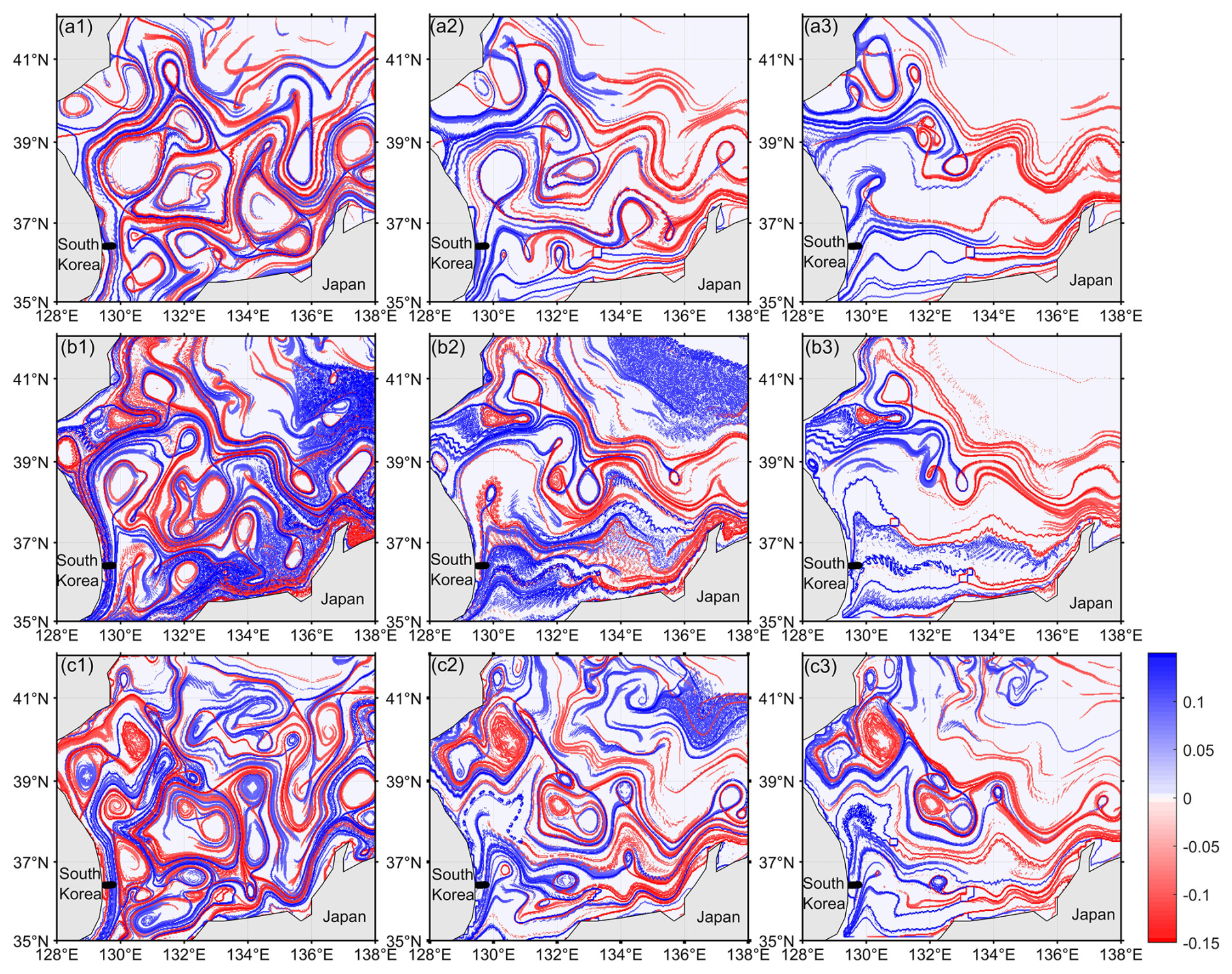
Figure 10 Finite-time Lyapunov exponent (FTLE) structures computed from one-week-averaged velocity fields. The panels show FTLE fields for (a1) u_G, (a2) ${\mathit{u}}_{\mathrm{G}}+{\mathit{u}}_{\mathrm{E}}+{\mathit{u}}_{\mathrm{S}}$, (a3) ${\mathit{u}}_{\mathrm{G}}+{\mathit{u}}_{\mathrm{E}}+{\mathit{u}}_{\mathrm{S}}+{\mathit{u}}_{\mathrm{W}}$, (b1) CMS, (b2) CMS-w1, (b3) CMS-w1-st, (c1) HYC, (c2) HYC-w1, and (c3) HYC-w1-st. Here, u_G, u_E, u_S, and u_W denote geostrophic current, Ekman current, Stokes drift, and windage, respectively. CMS denotes the GLORYS reanalysis distributed by Copernicus Marine, and HYC denotes the GOFS analysis based on HYCOM.

The data-driven velocity fields showed a clear transport-separating FTLE structure near the early bifurcation region off the eastern Korean coast. In particular, the geostrophic current field and the data-driven combined velocity fields retained a ridge structure in which attracting and repelling FTLE ridges were closely aligned or intersected near the region where the observed drifter trajectories initially separated. This structure is consistent with a hyperbolic-type bifurcation region rather than a mathematically exact, stationary hyperbolic point. Because the drifters were released close to this Lagrangian transport boundary, small differences in initial position and forcing could separate the particles into different pathways: one following the coastal northward route along the East Korea Warm Current and the other moving offshore and subsequently eastward.

In contrast, the CMS- and HYC-based FTLE fields did not show a comparable hyperbolic-type ridge intersection in the same region. The model-derived FTLE structures were smoother, weaker, or spatially displaced relative to the data-driven FTLE structure. Adding windage and Stokes drift to the CMS and HYC velocity fields changed the magnitude and direction of particle advection, but it did not reconstruct the same transport-separating FTLE pattern near the release region. This explains why the model-derived simulations could not reproduce the early pathway separation as accurately as the optimized data-driven forcing combination.

The FTLE comparison therefore supports the trajectory-based evaluation in Table 4. The improved performance of the data-driven approach does not imply that the GOFS analysis or GLORYS12V1 reanalysis lack geostrophic dynamics. Both products assimilate sea-level information, but their surface velocity fields are dynamically adjusted by the model physics, data-assimilation scheme, vertical mixing, spatial resolution, and temporal averaging. Rather, the result indicates that the early drifter bifurcation was highly sensitive to the local structure of the near-surface velocity field. The data-driven geostrophic-based forcing combinations better preserved the FTLE ridge structure associated with this bifurcation region, whereas the HYC and CMS velocity fields smoothed or displaced the local transport boundary. Consequently, once the simulated particles selected an incorrect pathway during the first stage of transport, the downstream separation error increased rapidly, leading to larger MAE and lower NCLS values over the full trajectory.

Overall, the comparison with HYC and CMS confirms that the key advantage of the optimized data-driven forcing is not only the inclusion of additional windage or Stokes drift, but also the ability to reproduce the local Lagrangian transport structure controlling the early bifurcation of the drifter pathways. This finding emphasizes that accurate representation of transport-separating structures near the release region is essential for predicting the fate of near-surface floating particles in the East/Japan Sea.

4.2 Seasonal variation of atmospheric and oceanic forcings

The seasonal variation of waves and winds that potentially influence the transport of floating debris is illustrated in Fig. 11. Both significant wave height (SWH) and wind speed follow a clear seasonal pattern, increasing in the order of summer (June–August), fall (September–November), spring (March–May), and winter (December–February). During fall and winter (Fig. 11g and h), the EJS is subject to persistent and strong northwesterly winds, which generate significantly higher wave heights near the Japanese coastline due to fetch-limited wave development from the Korean Peninsula (Chen et al., 2002; Park et al., 2005; Ebuchi, 1999). Monthly averaged satellite-derived SWHs show a pronounced seasonal variability, with high values exceeding 2.5 m in winter and low values below 1 m in summer (Woo and Park, 2017), consistent with the seasonal averages depicted in Fig. 10. This spatial asymmetry in wave height enhances wave-driven surface transport (Stokes drift) toward the Japanese coast during winter. The mean winter SWH reaches 1.68 m, with a maximum of 2.58 m. In contrast, during summer, the mean SWH decreases to 0.55 m, with a peak of 0.82 m, and wave propagation is influenced by prevailing southerly winds, which tend to shift northward.

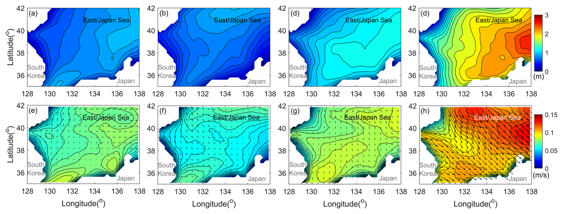
Figure 11 The mean of significant wave height (a–d), wind (e, f) in EJS for each season in 2021: (a, e) spring (1 March–30 May), (b, f) summer (1 June–30 August), (c, g) autumn (1 September–30 November), and (d, h) winter (1 December–28 February).

Like the distinct seasonal variations in wave and wind strength and direction, the direct forcings driving surface debris transport also exhibited marked seasonal variability. Figure 12 presents the absolute and relative magnitudes of the forcing components for PTM-DX (Fig. 12a and c) and PTM-DO (Fig. 12b and d). For PTM-DX forcings, the geostrophic current was the dominant component year-round, contributing approximately 68 % of the total forcing in summer and declining to around 48 % in winter. Among the remaining components, windage and Stokes drift made comparable contributions, both substantially exceeding that of the Ekman current across all seasons. Similarly, for PTM-DO, the geostrophic current remained the primary forcing component, contributing about 83 % in summer and decreasing to roughly 65 % in winter. The other three components, windage, Stokes drift, and Ekman current, had similar magnitudes, particularly during winter. However, Stokes drift was generally less influential than windage and Ekman current, likely due to its more rapid exponential decay with dept  (e^−2kz), in contrast to the slower decay of the Ekman current ($e^{-z/d}$). The estimated Ekman depth ranged from approximately 15 m in summer to 30 m in winter, substantially deeper than the depth affected by Stokes drift. Consequently, the absolute magnitude of the Ekman current contribution showed little variation between PTM-DX and PTM-DO.

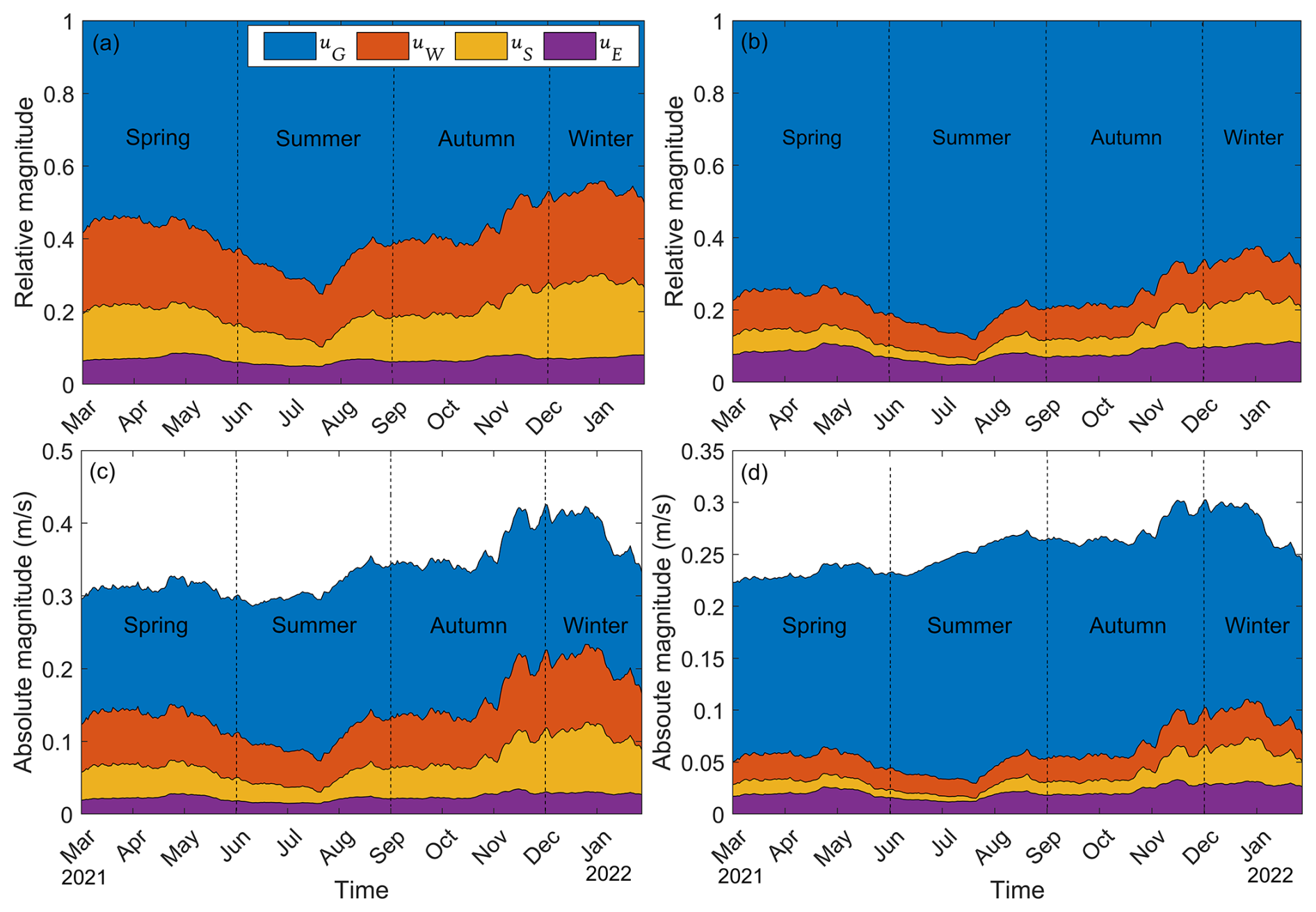
Figure 12 The relative and absolute value of the current components at the surface (a, c) and 1.5 m depth (b, d) of (u_G – geostrophic current, u_W – wind-driver current, u_S – Stoke current and u_E – Ekman current) from March 2021 to February 2022.

The PTM results indicate that the optimal current representation for tracking DX drifters is achieved using three components: geostrophic current, Stokes drift, and windage. This combination performed slightly better than the full four-component setup, suggesting potential redundancy or overestimation when the Ekman current is included in modelling surface debris transport. In contrast, the optimal configuration for PTM-DO involved all four components, indicating that at subsurface depths, overlap among wind-driven forcings, such as windage, Stokes drift, and the Ekman current, is reduced, and their combined influence is necessary to achieve the best performance.

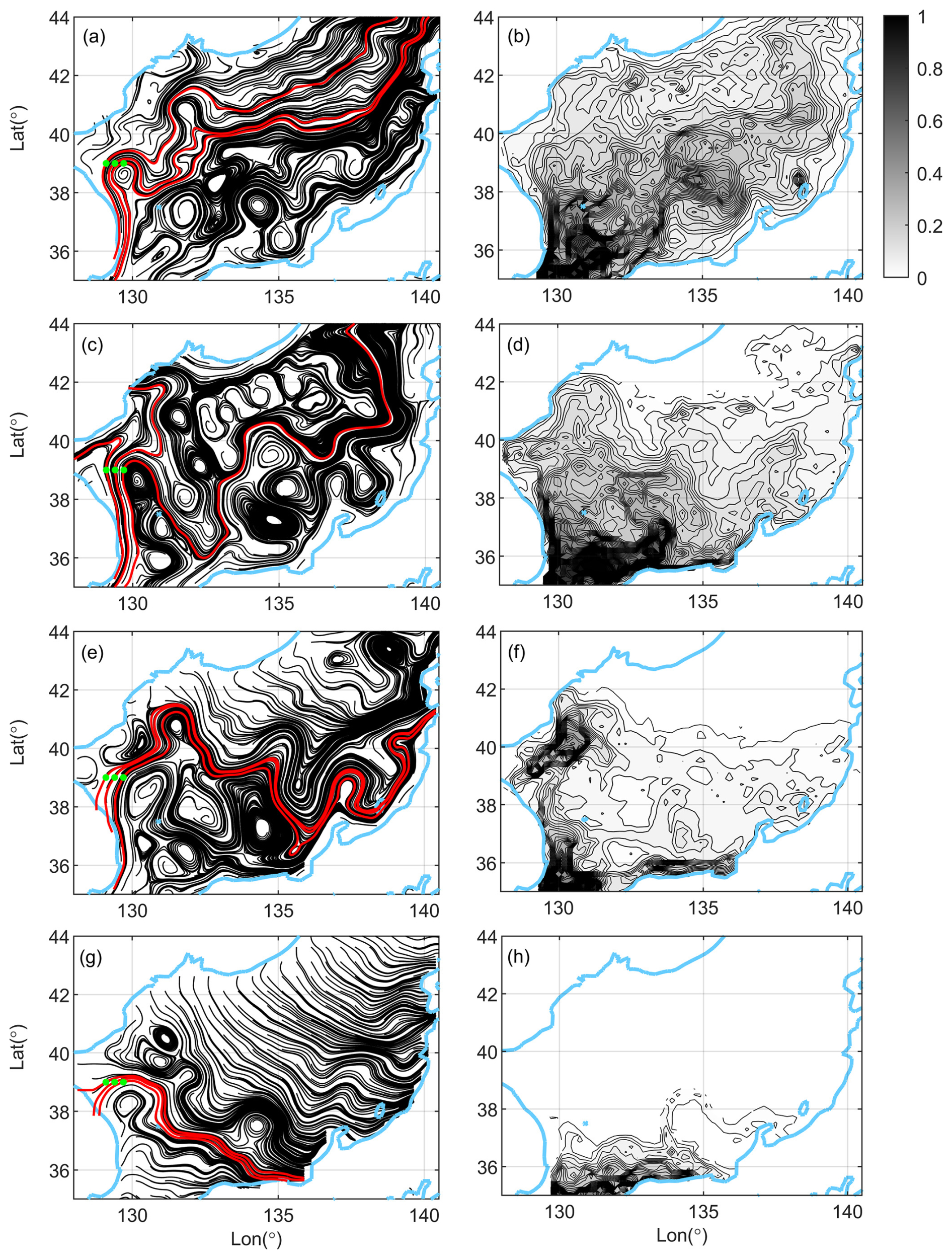
Figure 13 Seasonal streamlines and particle accumulation maps from March 2021 to February 2022, simulated using the optimal forcing combination (C7). Panels (a), (c), (e) and (g) show streamlines of the seasonally averaged surface current for spring (March–May), summer (June–August), autumn (September–November), and winter (December–February), respectively. Panels (b), (d), (f) and (h) show the corresponding seasonal particle accumulation maps. Red lines represent streamlines that pass through three fixed points marked in green. Particles were released every five days from March 2021 to February 2022 at the southwestern entrance of the EJS and tracked for five months. The accumulation maps display the relative frequency of particle occurrence, calculated as the number of particle passages through each 5 km grid cell normalized by the maximum frequency.

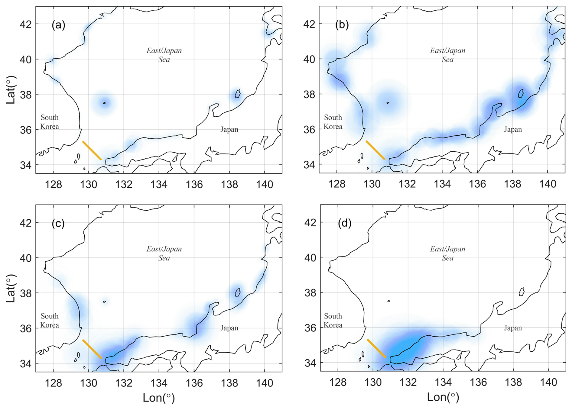
Figure 14 Spatial distribution and relative accumulation intensity of beached particles simulated using the optimal surface forcing (C7) for (a) spring (March–May), (b) summer (June–August), (c) fall (September–November), and (d) winter (December–February). The beached particle locations were determined from the same particle trajectories used in Fig. 13. Beaching is defined as the behavior of particles first contacting the coastline. The particle release location is marked by the yellow line. Color intensity along the coastline indicates the relative density of particle accumulation, with darker shades representing higher accumulation.

4.3 Seasonal variation of particle transport and dispersion

The seasonal variation of atmospheric and oceanic forcings near the air–sea interface, as described in the previous section, plays a key role in determining the fate of floating debris in the EJS. To investigate the seasonal variability in floating debris dispersion and transport driven by surface forcings, a particle tracking model was run using the optimal forcing combination for DX drifters (C7). A total of 576 particles were released at the ocean surface near the southwestern entrance to the EJS, with releases occurring every five days throughout the year (March 2021 to February 2022), and each particle was tracked for five months. Figure 13 presents streamlines based on seasonally averaged velocity fields (Fig. 13a, c, e and g), along with the corresponding seasonal particle accumulation maps (Fig. 13b, d, f and h), showing the relative frequency of particle presence within 5 km grid cells. The three red streamlines highlight trajectories passing through the same points along the eastern side of the subpolar front near 40° N.

In spring (Fig. 12a and b), the streamlines reveal that relatively strong winds blow northward near the Korean Peninsula and shift northeastward, especially in the northern EJS, facilitating material transport along and above the subpolar front. This wind-driven configuration results in the broadest dispersion of floating debris among all seasons. In summer (Fig. 12c and d), the flow is characterized by eddy-like coherent patterns throughout the EJS, driven by persistent mesoscale circulations under the weakest wind conditions. A branch of the EKWC flows northward along the coast and forms a closed streamline loop in the northern coastal region. This circulation pattern suggests that particles entrained on the western side of the EKWC become trapped and accumulate along the Korean coastline. In fall (Fig. 12e and f), streamlines originating from the northern coastline extend southeastward across the northern EJS. The red streamlines show minimal variation, indicating relatively slow northward particle movement. This is consistent with the broader, lower-concentration particle distributions observed in the accumulation map. Additionally, the streamlines near the Japanese coastline remain open, allowing debris to continue along the coast. In winter (Fig. 12g and h), most streamlines appear nearly straight, influenced by strong and consistent west-northwesterly winds and wave propagation in the same direction. As a result, particle trajectories are largely confined to the southern EJS. Given that our drifters were released in mid-November and tracked for several months, the fall and winter transport maps (Fig. 12e–h) effectively represent the observed fate of drifters that eventually beached along the Japanese coastline.

The seasonal beaching locations of particles are illustrated in Fig. 14, where beaching is defined as particle contact with the coastline. In spring (Fig. 14a), the number of beached particles was the lowest among all seasons, with a substantial portion remaining offshore. This pattern corresponds with the springtime streamline plots, which show predominantly northeastward transport across the EJS and limited streamline closure near the coast. In summer (Fig. 14b), when winds were weakest, the widest spatial distribution of beaching was observed, with particles reaching both the Japanese and Korean coastlines surrounding the EJS. Fall (Fig. 14c) was characterized by concentrated beaching along the southern coasts of both Japan and Korea, with particularly pronounced accumulation along the Japanese coastline. In winter (Fig. 14d), strong northwesterly winds likely contributed to increased beaching intensity along the southern Japanese coast. These seasonal mechanisms align with previous numerical studies: Yoon et al. (2010) highlighted the dominant role of monsoonal winds and windage in driving seasonal peaks of floating debris accumulation along the Japanese coast, while Iwasaki et al. (2017) demonstrated that intensified winter wave conditions and associated Stokes drift significantly enhance the onshore transport of buoyant debris toward Japan.

The seasonal variation in relative dispersion can also be interpreted in terms of atmospheric and oceanic forcings (Fig. 15). In all cases, dispersion initially exhibited a brief period of slow growth, attributed to the model's constant diffusivity within grid cells, followed by a more rapid increase consistent with Richardson-like behavior, continuing until approximately 30 d after release. During this phase, particles released in winter showed the lowest relative dispersion, while those released in summer exhibited the highest. The reduced dispersion in winter likely resulted from persistent strong winds and waves that constrained particle motion, leading to concentrated beaching along the southern Japanese coast (Fig. 14d). In contrast, the enhanced dispersion in summer was attributed to weak winds, resulting in reduced wave action, Stokes drift, and Ekman currents, which allow mesoscale eddies to dominate particle transport. This pattern aligns with Fig. 14b, which shows widespread beaching along both the Korean and Japanese coastlines. Over time, relative dispersion in all seasons began to plateau roughly one month after release, as particle pair separations approach the basin scale. These results suggest that strong winds suppress the influence of mesoscale eddies by restructuring the flow into a more uniform, wind-driven (ballistic-like) velocity field, whereas weak winds allow particles to remain entrained within mesoscale eddies, thereby enhancing basin-wide dispersion, especially in marginal seas like the EJS.

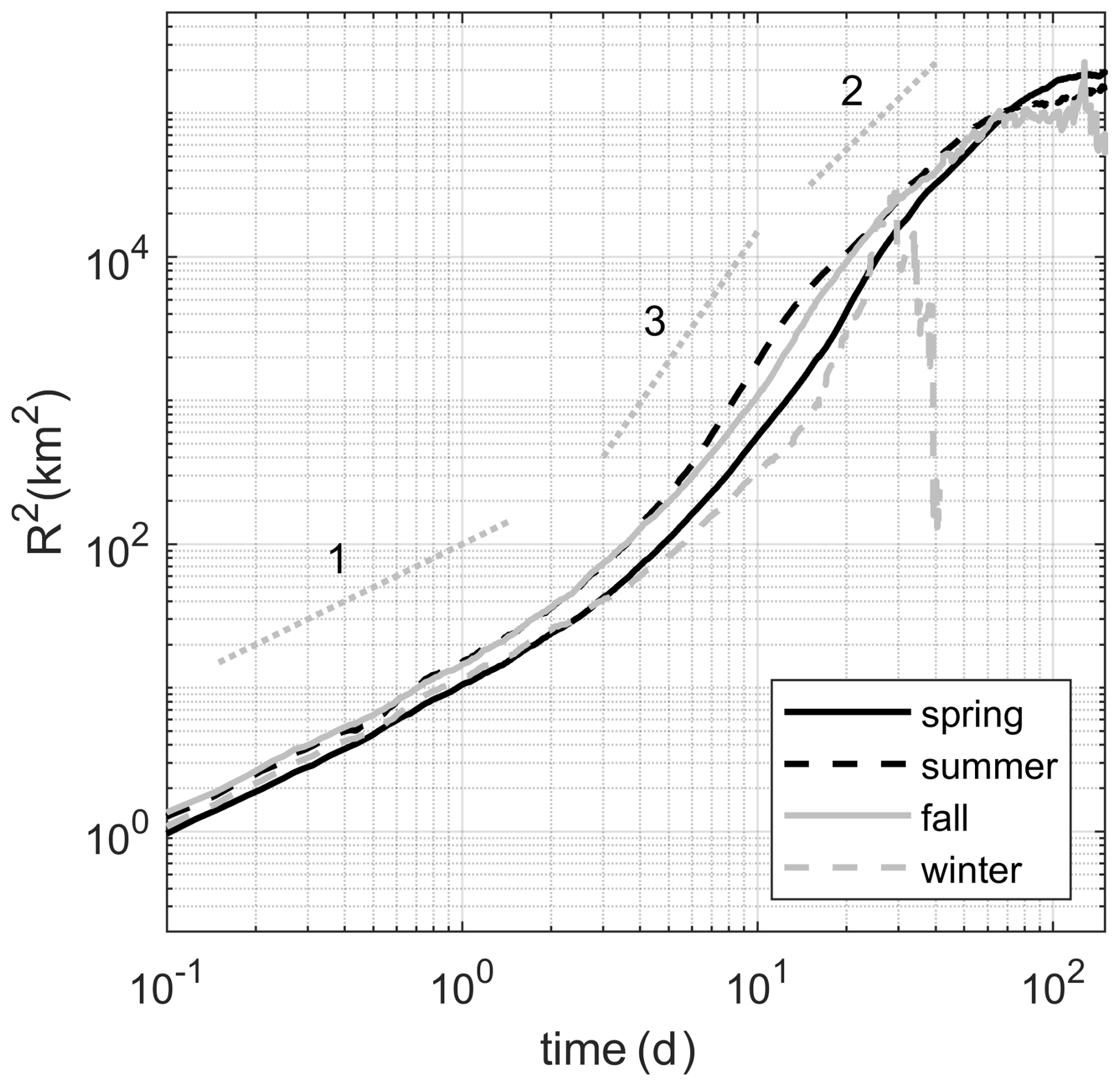
Figure 15 Seasonal variation of relative dispersion, R²(t), for particles (same as those used in Figs. 13 and 14) simulated using the optimal forcing combination (C7). Lines indicate relative dispersion for particles released in spring (black solid), summer (black dashed), autumn (gray solid), and winter (gray dashed).

5 Conclusions

This study evaluated the near-surface forcing combinations required to reproduce observed drifter trajectories in the East/Japan Sea using a passive particle tracking model driven by prescribed Eulerian velocity fields and a simple random-walk representation of unresolved diffusion. The 2021 drifter experiment revealed a clear cross-basin transport pathway from the Korean coast toward Japan, with the observed trajectories separating near a hyperbolic-type Lagrangian structure.

The comparison between observed and simulated trajectories showed that the optimal forcing combination depends on drifter type and effective sampling depth. For the undrogued DX drifters, the best performance was obtained by combining geostrophic current, Stokes drift, and windage. For the drogued DO drifters, the inclusion of all four components, geostrophic current, Ekman current, Stokes drift, and windage, provided the best agreement with observations. These results indicate that wave-induced drift and direct wind forcing are essential for surface-exposed objects, whereas Ekman current becomes more important for particles with a deeper effective sampling depth.

The optimized data-driven forcing combinations also performed better than the benchmark simulations driven by the GOFS analysis and GLORYS reanalysis in this specific experiment. The FTLE comparison suggests that the reconstructed forcing fields better represented the Lagrangian structure associated with the early drifter bifurcation. This does not imply general superiority over ocean analysis or reanalysis products, but shows that explicitly combining near-surface forcing components at physically relevant depths can improve trajectory prediction for this event.

Seasonal simulations showed that winter winds accelerate eastward transport and enhance beaching along the Japanese coast, whereas weaker summer winds allow mesoscale eddies to broaden particle dispersion and produce more spatially distributed beaching patterns. These results highlight the seasonal control of wind, waves, and mesoscale circulation on near-surface transport in the EJS.

The present PTM should be interpreted as a model of the fluid-dynamical component of near-surface particle transport, not as a complete fate model for specific macroplastic or microplastic debris. Processes such as fragmentation, biofouling- or colonization-induced buoyancy change, aggregation, degradation, vertical mixing, settling, resuspension, and detailed shoreline interaction were not explicitly included. Applications to real plastic debris would therefore require additional particle-specific terms depending on particle size, shape, density, material, buoyancy, and aging. Nevertheless, this study provides a physically constrained basis for improving debris-transport modeling in the EJS and other marginal seas.