Intraseasonal variability and eddy-induced structural modulation of the North Pacific intermediate water revealed by multi-mooring observations

The North Pacific Intermediate Water (NPIW) plays an important role in regulating thermohaline structure and biogeochemical distributions in the North Pacific. However, limited continuous observations have hindered our understanding of its short-term variability and structural response to mesoscale processes. Based on 1 year mooring observations from three sites (M1–M3) in the western North Pacific, this study investigates the intraseasonal structural variability of the NPIW and its modulation by mesoscale eddies. The NPIW thickness exhibits pronounced intraseasonal variability, with a dominant period of approximately 60–80 d that is coherent among the three mooring sites. Unlike previous studies that mainly focused on temperature and salinity anomalies, this study introduces NPIW thickness as a structural diagnostic parameter to characterize the vertical compression and expansion of the intermediate layer associated with mesoscale variability. The results reveal a clear inverse relationship between NPIW thickness and salinity, indicating that anticyclonic conditions are generally associated with thinner and more saline intermediate layers, whereas cyclonic conditions correspond to thicker and relatively fresher layers. Spatial composite analyses further show that thickness and salinity responses exhibit clear regional differences, with stronger variability near the western boundary, likely related to complex water-mass redistribution and possible mixing processes. These findings provide quantitative observational evidence for intraseasonal variability in NPIW thickness and highlight its usefulness as a diagnostic indicator for mesoscale–intermediate water interactions in the North Pacific.

1 Introduction

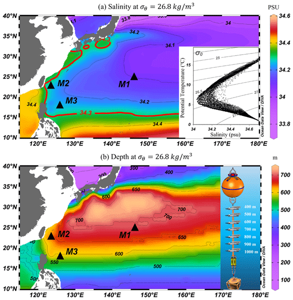
The North Pacific Intermediate Water (NPIW) is a pivotal component of the North Pacific's water mass and extensively studied due to its significant role in climate dynamics and oceanic processes (Talley, 1993; Masuda et al., 2003; You, 2003; Gong et al., 2019; Nishioka et al., 2020). This water mass originates in the northwestern subtropical gyre, within the transition zone between the Kuroshio Extension and the Oyashio front (Fig. 1). The NPIW is characterized by a salinity minimum of about 34.1–34.3 and relatively cool temperatures at depths of approximately 400–1200 m, with its core density centered around the 26.8σ_θ isopycnal. (Talley, 1993; Talley et al., 1995; Yasuda, 1997; You, 2003; Masujima and Yasuda, 2009). NPIW is a key component of the intermediate circulation in the North Pacific and plays an important role in ventilating the thermocline and intermediate layers (Talley et al., 1995; You, 2003). It forms the prominent salinity minimum layer and contributes to the redistribution of heat, freshwater, and dissolved substances such as oxygen and nutrients (Talley, 1993; Hansell et al., 2002; Auad et al., 2003; Zhou et al., 2021). Variability in NPIW can therefore influence both physical circulation and biogeochemical processes in the mid-depth ocean (Tsunogai, 2002; Ohkushi et al., 2003).

The distribution and transport pathways of the NPIW have been a focal point of oceanographic research. Many studies have shown that the NPIW is widely distributed in the North Pacific and is transported through complex water-mass pathways and circulation systems (Qiu, 1995; Ueno and Yasuda, 2003; Yasuda, 2004; Gordon and Fine, 1996; Kashino et al., 1996; Kashino et al., 1999; Yuan et al., 2022). You (2003) found that NPIW originates from the subpolar regions of the North Pacific and propagates through the eastern subtropical gyre towards the Indonesian Through flow. As a result, NPIW can be found in eastern Japan, eastern Taiwan, the West Philippine Basin, and the intermediate region of the North Pacific Ocean, and exhibits clear regional differences in its vertical distribution (You, 2003; Fujii et al., 2013). To provide hydrographic background for the present mooring observations, we used WOA data to illustrate the climatological distribution of NPIW in the study region (Fig. 1). The resulting distribution is generally consistent with previous studies, showing that NPIW is relatively shallow near the western boundary and deeper in the interior North Pacific. Since NPIW is one of the most important water masses in the global ocean, most of studies focus on its seasonal, interannual or interdecadal variations in different regions, and this variability is largely influenced by multi-scale ocean-atmosphere interactions (Masuda et al., 2003; Ohshima et al., 2010; Bingham and Lukas, 1995; Solomon et al., 2003; Qiu and Chen, 2011; Van Scoy and Druffel, 1993; Sugimoto, 2022; Li et al., 2023). However, most previous studies have focused on variability over seasonal to interannual or longer timescales, using hydrographic observations, climatological datasets, Argo profiles, reanalysis products, or numerical models. In contrast, direct long-term observations with sufficiently high temporal resolution remain limited in the intermediate ocean, where the NPIW is located. Moreover, salinity structures in the intermediate layer are not always accurately represented in gridded or model-based products, which may limit their ability to resolve short-term water-mass variability. Therefore, the intraseasonal variability of the NPIW and its structural response to mesoscale processes remain insufficiently understood.

Mesoscale eddies are widely found in the oceans, with lifetime ranging from a few days to several hundreds of days, and radii of up to several hundreds of kilometers in the mid latitude (Wyrtki et al., 1976; Richardson, 1983; Robinson and Leslie, 1985; Chelton et al., 2007; Chelton et al., 2011a, b; Zhang et al., 2014; Wunsch, 2007; Martínez-Moreno et al., 2021). A large number of observational studies have shown that eddies can affect depths of up to kilometers, that there are significant differences in the three-dimensional structural features within anticyclonic and cyclonic eddies, and that mesoscale eddies produce different temperature and salinity anomalies by causing uplift or subsidence of the isopycnals (Zhang et al., 2015; Thoppil et al., 2011; Zhang et al., 2016; Zhang et al., 2015; George et al., 2021; Waite et al., 2016; Hausmann et al., 2017). Within the range of NPIW generation, propagation and distribution, there is also a high incidence of mesoscale eddies, it is therefore of great interest to investigate whether mesoscale eddies have an impact on the NPIW in different regions and with different thermohaline characteristics. In a localized area along the western boundary, Mensah et al. (2015) examines the intraseasonal to seasonal variability of intermediate water east of Luzon and Taiwan by hydrographic data from several cruises, it deduced a possible relationship between the eddies and the intermediate water from SLA data. Also, Wang et al. (2016) revealed that the semiannual variability of water masses at the northern and southern hemispheric convergence near 8° N related to mesoscale eddies. Next, Ren et al. (2022) found an intraseasonal variability of the intermediate water of ∼ 80 d from direct observations of the subsurface moorings east of Taiwan, and that this variability is associated with mesoscale eddies. These studies reveal the complex variability of NPIW in the western boundary region, which may be extensively influenced by local water masses such as the South China Sea Intermediate Water Mass and the Kuroshio Intermediate water mass. Also these studies can illustrate some of the effects of eddies on intermediate water, but they are insufficient to demonstrate the widespread and persistent existence of NPIW's intraseasonal variability characteristics, which is one of the most important links between high-frequency variability and climate-scale cycles of change.

Previous studies have significantly advanced the understanding of the formation, distribution, and variability of the NPIW. However, most of these studies have primarily focused on temperature and salinity anomalies, offering limited insight into the structural response of NPIW to dynamic processes such as mesoscale eddies. As noted by Nakanowatari et al. (2015), model-based analyses often exhibit large uncertainties due to the scarcity of long-term in situ data, constraining their ability to accurately represent the vertical structure and temporal evolution of NPIW. These limitations highlight the necessity of direct, continuous mooring observations to resolve intraseasonal processes that can strongly influence the intermediate-layer structure and mixing. To address these gaps, the present study introduces intermediate water thickness as a structural diagnostic parameter to characterize the physical adjustment of NPIW under mesoscale eddy forcing. Thickness, defined as the vertical extent of the low-salinity core, serves as an integrated indicator of baroclinic adjustment, isopycnal displacement, and mixing intensity. Moreover, variations in NPIW thickness can directly influence the vertical distribution of nutrients and dissolved oxygen, linking physical dynamics with mid-depth biogeochemical and ecological processes. Changes in the structural extent of NPIW may also modulate carbon storage and ventilation pathways, highlighting the broader climatic and ecological implications of mesoscale-driven structural variability in the intermediate ocean.

By combining long-term mooring observations from three distinct sites (M1–M3) across the western Pacific, this study provides the first quantitative evidence of intraseasonal variability in NPIW thickness and its strong inverse relationship with salinity. This structural perspective complements traditional thermohaline analyses and enables a more comprehensive understanding of how mesoscale eddies reshape the hydrographic properties and vertical structure of the NPIW.

2 Data and Methods

2.1 Mooring data

To investigate NPIW variability, three mooring systems were deployed in the northwestern Pacific (Fig. 1). The locations, observation periods, and equipment setups of these three moorings, M1, M2, and M3, are described as follows. The mooring M1 is located at 146° E and 25° N, with an observation period from April 2017 to June 2018; M2 is located to the east of Taiwan on the western boundary, at 122.67° E and 22.3° N, with an observation period from August 2019 to December 2020; while M3 is located at 126° E and 18° N, with an observation period from January 2016 to June 2017. Each mooring was instrumented with conductivity–temperature–depth sensors (Sea-Bird Electronics SBE 37) installed at 100 m vertical spacing between depths of 400 and 1000 m, with all instruments programmed to record data at 10 min intervals.

The deployment depths were carefully designed to span the upper and lower boundaries of the NPIW, ensuring adequate vertical coverage of its structure. The CTD data were first quality controlled before further analysis. Obvious abnormal values and isolated spikes were removed based on instrument records and physically reasonable ranges of temperature, salinity, and pressure. Because slight vertical movement of the mooring line may occur under strong currents, the recorded pressure data were used to determine the actual sampling depths of each CTD at each time step. To obtain uniformly gridded vertical profiles for subsequent analyses including contour plots and depth-dependent temperature and salinity, the observations were linearly interpolated between vertically adjacent CTD measurements on the same mooring line onto a common set of standard depth levels.

In addition, local linear interpolation was applied between vertically adjacent CTD sensors on the same mooring line that bracketed the 34.3 psu value to estimate the depths of the upper and lower isohalines used for NPIW thickness calculation. The thickness was then defined as the vertical distance between these two interpolated isohaline depths. After quality control and interpolation, the 10 min observations were averaged into daily means for all subsequent analyses.

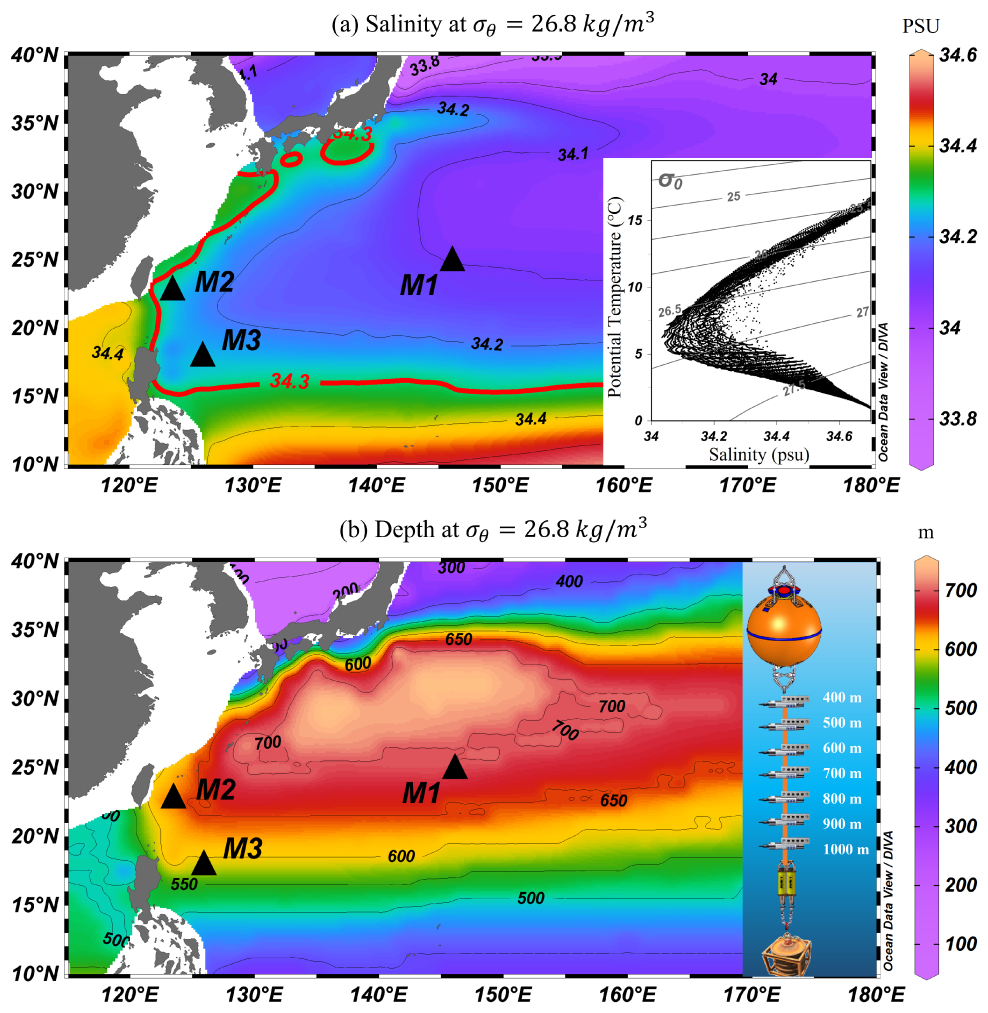
Figure 1 Distribution of salinity (a) and depth (b) along the 26.8σ_θ isopycnals at Northwestern Pacific. The T-S scatter plot in the lower-right corner of (a) illustrates the vertical distribution of NPIW. The color shading and black line in (a) and (b) represent the salinity and depth, respectively. The right-hand side of (b) shows a schematic diagram of the CTD deployment with mooring. The red contours of 34.3 psu is represent the NPIW range from Talley (1993) and You (2003). The black triangle is the mooring location: Mooring 1 (M1), Mooring 2 (M2) and Mooring 3 (M3). Salinity and depth in the Fig. 1 are taken from climatological averaged data from World Ocean Atlas 2023 (WOA23), NOAA National Centers for Environmental Information, and plot with Ocean Data View (Schlitzer, Reiner, Ocean Data View, https://odv.awi.de, last access: 28 July 2026, 2022).

2.2 World Ocean Atlas 2023

The spatial distribution of NPIW in the northwestern Pacific was examined using the World Ocean Atlas 2023 (WOA23). Produced by NOAA's National Oceanographic Data Center–Ocean Climate Laboratory (The data available online at: https://www.ncei.noaa.gov/products/world-ocean-atlas, last access: 28 July 2026), this dataset consists of objectively analyzed climatological fields derived from in situ observations, including temperature, salinity, dissolved oxygen, and inorganic nutrients at 102 standard depth levels in the global ocean (Reagan et al., 2023). Despite its broad distribution of NPIW, the definition of NPIW is not entirely uniform in previous studies. It has been identified using different criteria, including the salinity minimum, density ranges (typically 26.4–26.9σ_θ), and characteristic isohalines (Talley, 1993; You, 2000). These definitions emphasize different aspects of the same water mass, namely its core properties, dynamical layer, and vertical structure. Based on these previous studies, we use the WOA data to illustrate the climatological distribution of NPIW, as shown in Fig. 1. The spatial pattern is consistent with earlier findings (e.g., You, 2003), showing that the NPIW exhibits significant regional variability in its vertical structure. Specifically, the NPIW layer is relatively shallow in the western boundary region, while it deepens toward the interior of the North Pacific. This spatial variability provides an important background for interpreting the mooring observations in this study. In this study, these criteria are used in a complementary manner: the salinity minimum is used to describe the core property of the NPIW, the density range is used to characterize the intermediate dynamical layer, and the 34.3 psu isohaline is adopted to estimate the structural thickness of the low-salinity NPIW layer.

2.3 The Copernicus Marine Environment Monitoring Service (CMEMS) data

In this study, two Copernicus Marine Environment Monitoring Service (CMEMS) products were utilized.

2.4 Sea Level Anomaly (SLA) and Geostrophic Currents data

We used the Global Ocean Gridded L4 Sea Surface Heights and Derived Variables Reprocessed Dataset (E.U. Copernicus Marine Service Information, 2026a, https://doi.org/10.48670/moi-00145), provided by CMEMS (https://marine.copernicus.eu/, last access: 28 July 2026). This altimetry product merges multi-mission satellite observations and provides global gridded fields of sea level anomaly (SLA), absolute dynamic topography, and geostrophic currents. The data have a spatial resolution of $\mathrm{1}/\mathrm{4}$° and daily temporal resolution, covering the observation periods of all three subsurface moorings.

2.5 Temperature and Salinity Reanalysis Data

To analyze subsurface temperature and salinity variability around the mooring sites, we employed the Global Ocean Physics Reanalysis Product (E.U. Copernicus Marine Service Information, 2026b, https://doi.org/10.48670/moi-00052), a Level-4 global reanalysis distributed by CMEMS. This product provides three-dimensional fields of temperature, salinity, potential density, and geostrophic currents on a regular $\mathrm{1}/\mathrm{8}$° grid, spanning from the surface to 5500 m with 50 vertical levels. The product is generated by combining in situ and satellite observations on a global scale. The available record covers the period from January 1993 to the present, with temporal resolutions of weekly and monthly (Guinehut et al., 2012; Mulet et al., 2012).

3 Result

3.1 Hydrographic and temporal characteristics of NPIW

To gain an initial understanding of the NPIW characteristics at the locations of our three deployed moorings, we employed the WOA database to create decadal average maps of salinity and depth distribution on the 26.8σ_θ isopycnal, as illustrated in Fig. 1. The NPIW shows significant local variability, with the NPIW showing lower salinity values and its core depth of approximately 34.1 psu and 700 m near M1 mooring site, respectively. NPIW in the western and southern parts of the distribution, the minimum salinity of the NPIW increases and its depth is relatively shallow. Near the M2 mooring location, the low salinity value and depth adjust to about 34.25 psu and 600 m, respectively. Based on the NPIW range determined by the 34.3 psu contour of the salinity definition, M3 near 18° N, which can be seen in Fig. 1 to be located close to the south edge of the NPIW distribution, has a salinity minimum value close to that at M2, but the depth of the low salinity core becomes further shallower to ∼ 550 m. Thus, the moorings utilized in this study have effectively observed NPIW, capturing its significant spatial and temporal variability across different regions.

Observations from the M1 mooring over more than a year, as shown in Fig. 2a, reveal that the low salinity core of the NPIW has an average depth of approximately 700 m, fluctuating within the range of 26.4 to 27σ_θ isopycnal, with the minimum salinity value being around 34.15 psu. The observed salinity minima at M1 were also found to be slightly higher compared to the climatological averaged data showed in Fig. 1a. Additionally, significant temporal variations in salinity were observed at depths of 400–900 m by the M1 mooring. The M2 mooring located east of Taiwan near the western boundary, observed salinity below 400 m as depicted in Fig. 2c. The low salinity core varied between the 26.6–26.8σ_θ isopycnals showing more significant changes than those observed at M1, with average minimum salinity values and depths of approximately 34.2 psu and 600 m, respectively, which are higher than the minimum salinity values observed at the M1 location. And it is interesting to note that the low salinity core of M2 is apart, such as the salinity measured in April–May 2020 in Fig. 2c, which is close to 33.6 psu, splitting the low salinity core with a salinity value of around 34.2 psu. At the more southerly M3 mooring, as illustrated in Fig. 2e, the low salinity core also apart with seven significant low salinity events observed over a year. The average minimum salinity value between the 26.6–26.8σ_θ isopycnals was 34.3 psu, with corresponding temperatures and depths of approximately 8 °C and 550 m, respectively. A distinctive feature of M3 was that the depth of the NPIW's low salinity core was shallower than that at M1 and M2, and the minimum salinity was significantly higher than M1 and M2. The results of NPIW observed by the three differently positioned subsurface mooring are basically consistent with the spatial distribution characteristics of NPIW in the North Pacific Ocean in the WOA data.

Upon comparing Fig. 2a, c, and e, it appears that the intermediate water masses at the M2 location exhibit greater variability, while those at the M1 location show relatively weaker variations. From the corresponding salinity standard deviation plots (Fig. 2b, d, and f), it is observed that the M1 mooring displays the smallest standard deviation at the NPIW core depth of approximately 700 m, indicating higher stability in intermediate layer salinity. Conversely, the salinity at the levels of NPIW for M2 and M3 shows greater variability. The largest standard deviation in salinity at the mooring M2 is 0.06 psu at around 600 m, shown in Fig. 2d, while a significant standard deviation in salinity around 0.03 psu is observed between 500–600 m from mooring M3. This variability in salinity in intermediate layer is also depicted in the T-S (Temperature-Salinity) plot in Fig. 3, where the range of salinity changes at the mooring M2 is the largest among the three observed locations, ranging from 34.13 to 34.35 psu, with M1 showing the smallest variation. Differences in standard deviations also illustrate the variability of NPIW changes across regional locations, with the least variability at 25° N, possibly related to its deeper depth. The relatively strong intermediate-layer salinity variability near M2 is likely associated with complex local circulation, where intermittent influences of South China Sea Intermediate Water (SCSIW), a salinity-minimum water mass (∼ 34.4 psu at ∼ 500 m) are modulated by the Kuroshio and mesoscale eddies (Mensah et al., 2015; Ren et al., 2022). Overall, the measurements from the subsurface moorings show a change in the minimum salinity in the mid-ocean region, which also corresponds to a salinity within the range defined by the NPIW, and this change also reflects the fluctuations in low salinity core of the NPIW.

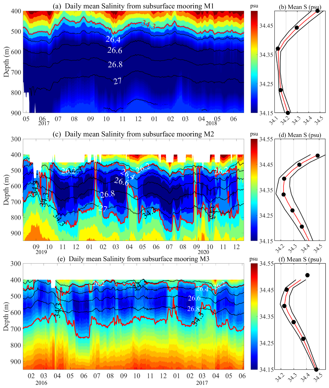
Figure 2 The observation of salinity from subsurface mooring. (a), (c) and (e) represent time series plots of salinity measured at different observation times for the three moorings, respectively. M1 is observed from April 2017–June 2018, M2 is observed from August 2019–December 2020 and M3 is observed from January 2016–June 2017. Color shading and the black lines represent the salinity and 26.2 to 27.0σ_θ isopycnal, and also red line represent the 34.3 psu in (a), (c) and (e), respectively. In (b), (d) and (f), the red line and black line represent the mean salinity and standard deviation of salinity over the observation period, respectively. The black circle in (b), (d) and (f) are represents the average depth of deployed CTDs in subsurface moorings.

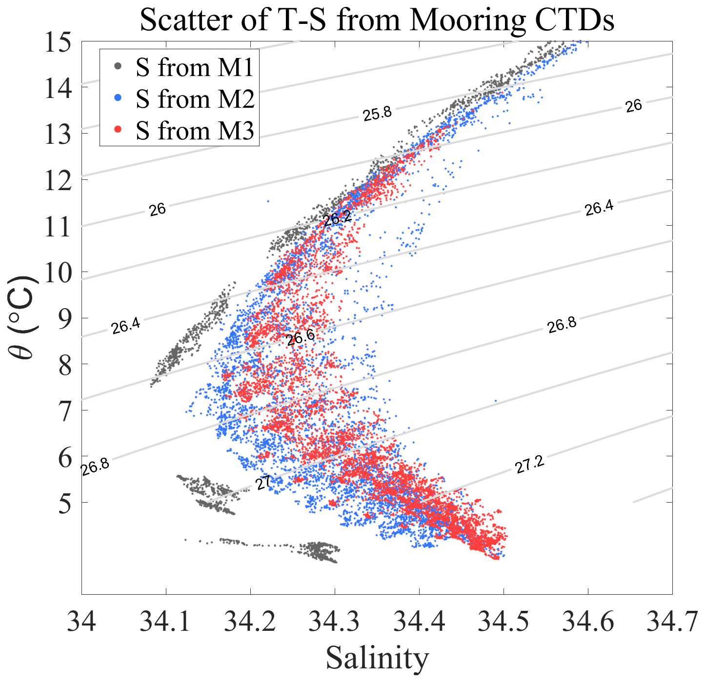
Figure 3 (a) The Temperature-Salinity plot from mooring CTDs. The black, green and red points are represent the M1, M2 and M3 measurements temperature and salinity, respectively.

3.2 Intraseasonal Variations of NPIW Thickness and Salinity

Given that salinity alone cannot fully capture the structural variability of the NPIW, this section examines the variations in both layer thickness and isopycnal-averaged salinity to better characterize its dynamic evolution. The mean salinity within the 26.4–26.9σ_θ density range was used to characterize the intermediate-layer salinity variability associated with the NPIW. This density interval has been widely adopted in previous studies to represent the dynamical layer occupied by the NPIW and its surrounding transition waters (Talley, 1993; You, 2000; Yasuda, 2004). The NPIW thickness was estimated from the vertical distance between the upper and lower selected isohalines. At M2 and M3, the 34.3 psu isohaline was used as a tracer-based boundary for the low-salinity intermediate layer. This salinity threshold is not intended to define the entire NPIW water mass, but provides a consistent structural index for quantifying changes in the vertical extent of the low-salinity layer. At M1, the 34.2 psu isohaline was used instead of 34.3 psu because the low-salinity layer at this site is thicker and extends deeper than at M2 and M3. During part of the record, the lower 34.3 psu isohaline was located below the deepest CTD observations, preventing a continuous estimate of layer thickness without extrapolation. The 34.2 psu isohaline at M1 remains within the low-salinity NPIW layer and allows the relative expansion and compression of the local low-salinity core to be followed within the available observational range. Therefore, the absolute thickness at M1 should not be directly compared with the 34.3 psu-based thickness at M2 and M3, whereas its temporal variability remains useful for describing local changes in the intermediate low-salinity structure.

To assess the uncertainty associated with this isohaline-based thickness estimate, shipboard CTD salinity profiles near the mooring sites were used as high-vertical-resolution references. These profiles were not collected at exactly the same time as the daily moored observations, and therefore were not used to validate individual daily thickness estimates. Instead, they were used to examine how much uncertainty may be introduced by the vertical spacing of the moored CTD sensors and by the local linear interpolation between adjacent sensors. For each shipboard CTD profile, the upper and lower isohaline depths were first identified from the full-resolution salinity profile. The same profile was then represented only by salinity values at the nominal depths of the moored CTD sensors, and the isohaline depths were recalculated using the same interpolation procedure as that applied to the mooring records. The difference between the thickness obtained from the full-resolution profile and that obtained from the mooring-depth representation was taken as an estimate of the thickness uncertainty. This comparison gives estimated uncertainties of 6.79 m at M1, 11.30 m at M2, and 1.16 m at M3, with a mean value of 6.42 m. These values are much smaller than the main seasonal, inter-site, and mesoscale thickness variations discussed below. Nevertheless, because the shipboard CTD profiles are not time-matched to the daily moored records, short-term thickness variations of several tens of metres are interpreted cautiously.

Figure 4 presents the time series of NPIW thickness (red line) and average salinity between isopycnal surfaces (blue line) at three mooring sites (M1, M2, and M3). At M1 (Fig. 4a), during 2017–2018, the NPIW thickness generally fluctuated between 250 and 400 m, with an average around 300 m. The corresponding average salinity remained consistently below 34.2 psu, closely matching the typical NPIW characteristics. A pronounced minimum in salinity was observed in October–November 2017, coinciding with a local maximum in thickness exceeding 350 m. Compared with M2 and M3, the salinity variability at M1 was substantially weaker. This difference is likely related to the distinct hydrographic and dynamical environment at M1, where the NPIW layer is generally deeper and thicker. In this region, mesoscale variability mainly manifests as vertical displacement of isopycnals, while the surrounding horizontal salinity gradients are relatively weak compared with those near the western boundary. As a result, lateral redistribution and possible mixing of higher-salinity waters are less pronounced, leading to smaller salinity anomalies at M1.

At M2 (Fig. 4b, 2019–2020), the NPIW thickness exhibited more dramatic fluctuations, varying abruptly between 0 and 350 m. Notably, in October 2019, and February and September 2020, the thickness dropped from around 300 m to nearly zero, accompanied by a sharp increase in salinity exceeding 34.35 psu. This suggests a rapid erosion or replacement of intermediate water properties, likely driven by more active eddy activity or local mixing processes. At M3 (Fig. 4c) showed generally thinner NPIW, mostly between 100 and 250 m, with an average thickness of around 200 m. Similar to M2, the thickness at M3 was also marked by strong short-term fluctuations. Although the absolute thickness and salinity values varied across the three sites, all stations demonstrated consistent a clear and persistent inverse relationship between thickness and salinity. Periods of increased NPIW thickness were generally associated with decreased salinity. This structural variability implies that intermediate water changes may be modulated by local mesoscale eddies or mixing between water masses.

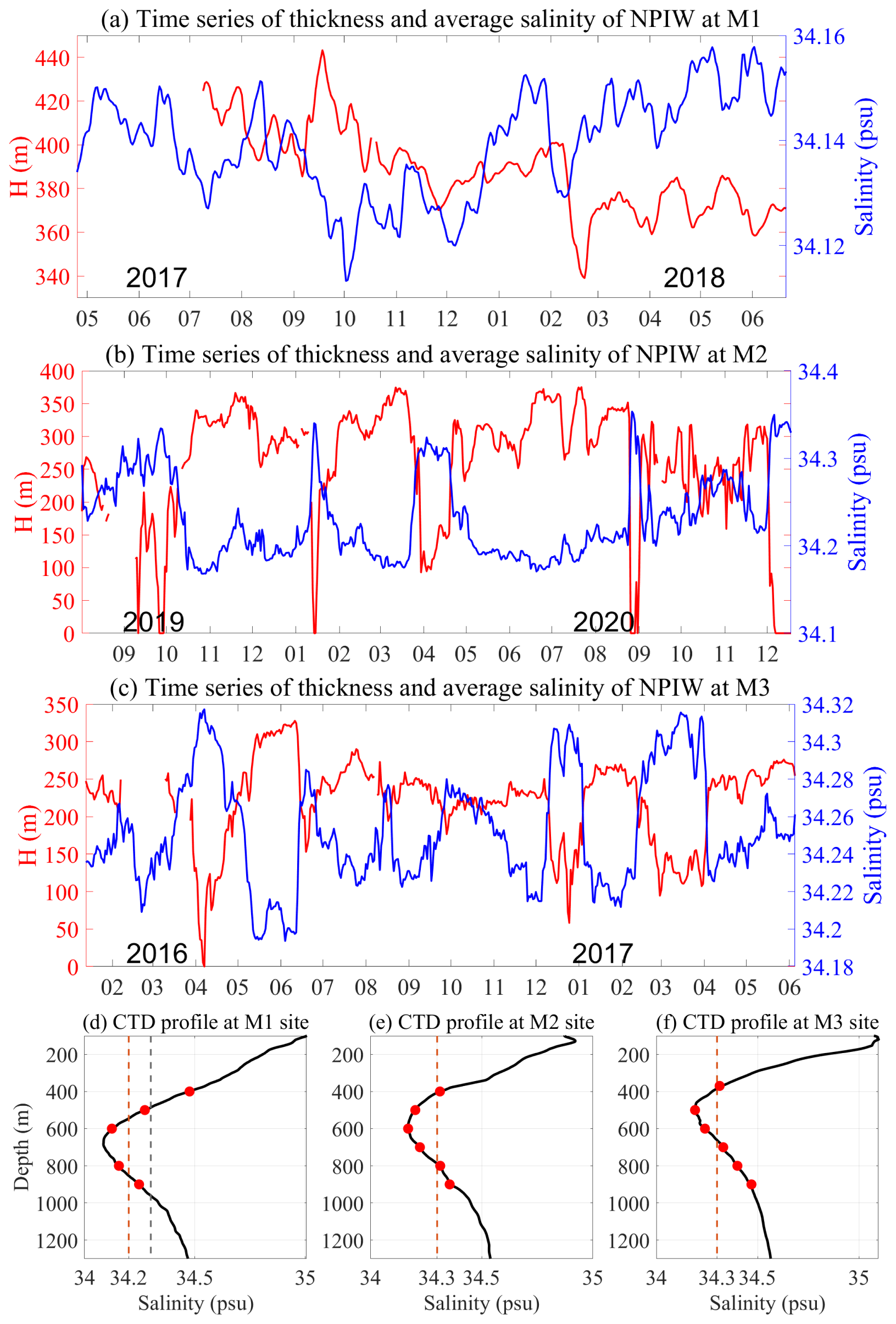
Figure 4 Time series of thickness and averaged salinity of NPIW at M1 (a), M2 (b) and M3 (c). The layer thickness was estimated as the vertical distance between the upper and lower selected isohalines. The 34.2 psu isohaline was used at M1, whereas the 34.3 psu isohaline was used at M2 and M3. The average salinity between the 26.4 and 26.9σ_θ isopycnal was used to represent the salinity characteristics of the NPIW. (d–f) Shipboard CTD salinity profiles near M1, M2, and M3, respectively. The black curves denote the full-resolution shipboard CTD salinity profiles, and the red circles indicate salinity values sampled from these profiles at the nominal depths of the moored CTD sensors. The orange dashed lines mark the selected isohaline used for estimating the thickness of the low-salinity intermediate layer: 34.2 psu at M1 and 34.3 psu at M2 and M3. The grey dashed line in panel (d) marks 34.3 psu for comparison. These profiles show a well-defined low-salinity intermediate layer and relatively smooth salinity variations across the selected isohaline intervals, supporting the use of local linear interpolation between adjacent moored CTD sensors.

To further investigate the temporal characteristics underlying the observed thickness and salinity fluctuations, particularly their dominant time scales, a wavelet analysis was performed on both salinity and thickness at each mooring site. As described in the previous section, the relationship between NPIW thickness and isopycnal-averaged salinity effectively captured the internal structural response of the intermediate layer. However, when examining temporal variability and dominant periodicities, a fixed-depth averaged salinity was used instead of isopycnal averaging. This approach allows the salinity signal to incorporate the vertical displacement of isopycnals induced by mesoscale eddies, thereby enabling a more direct comparison with the SLA time series and identification of intraseasonal oscillations. Different averaging definitions were adopted in this study according to the specific physical quantity being analyzed. The 26.4–26.9σ_θ density range was used to characterize the dynamical intermediate-water layer associated with the NPIW and to reduce the influence of vertical isopycnal displacement. In contrast, fixed-depth averages were used to describe local salinity variability within the observational range at individual mooring sites. For fixed-depth salinity analyses, different averaging ranges were adopted according to the local vertical distribution of the NPIW at each mooring site. The NPIW at M1 and M2 is generally deeper and thicker than at M3; therefore, the 500–800 m layer was used at M1 and M2, while the 500–700 m layer was used at M3. Initially, a unified depth range was considered for all sites. However, if the same depth range (e.g., 500–800 m) were applied to M3, the averaged salinity would include a larger contribution from deeper surrounding waters beneath the principal NPIW layer, thereby weakening the representativeness of the NPIW signal. The selected depth ranges were therefore adjusted to better capture the dominant low-salinity intermediate layer at each site.

Although the wavelet spectra were also calculated for NPIW thickness, the results exhibited nearly identical dominant periods and spectral power to those of salinity, confirming the tight coupling between thickness and salinity variations. Therefore, only the wavelet spectra of salinity are shown for brevity. The results at site M1 (Fig. 5a–b) indicate a pronounced intraseasonal variability with a dominant period of approximately 70–80 d, consistent with the SLA fluctuations observed in the same region. While this intraseasonal variation cycle exhibits temporal variability, it was more significant from May 2017 to April 2018, while the signal strength of the cycle significantly decreased after April 2018. Figure 5c–d represent the results of the wavelet analysis of averaged salinity at 500 to 800 m at M2, with a similar ∼ 80 d period as on the M1, the intraseasonal signals at M2 also exhibit variability during different observation periods. During the observation period from September 2019 to August 2020, the variability period appears to be longer about 80 d showing in Fig. 5c. The observation results from mooring M3 shown in Fig. 5e–f, indicate relatively stable intraseasonal variation periods of 70–80 d throughout the observation period.

These results collectively demonstrate that the structure and properties of the NPIW exhibit robust intraseasonal variability across different locations, reflecting a common intraseasonal signal that may be linked to regional mesoscale dynamics or other oceanic processes.

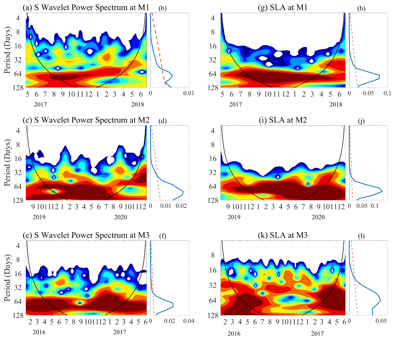
Figure 5 The wavelet power spectrum for salinity from 500 to 800 m at M1, from 500 to 800 m at M2 and from 500–700 m at M3 in (a), (c) and (e), respectively. (b), (d) and (f) are the corresponding global spectrum of salinity in (a), (c) and (e), with the red dashed line indicating the critical value at the 95 % confidence level. (g), (i) and (k) are the wavelet power spectrum for Sea Level Anomaly at the mooring site M1, M2 and M3, also the (h), (j) and (l) are the corresponding global spectrum of SLA.

3.3 Influence of SLA on the Salinity Structure of NPIW

In the previous section, a strong inverse relationship between NPIW layer thickness and isopycnal-averaged salinity was identified. This suggests that salinity can serve as an effective proxy for structural changes in the intermediate water layer. Therefore, in this section, we focus on the relationship between salinity and SLA, to indirectly assess the influence of mesoscale eddies on the structural variability of the NPIW. In the western North Pacific, mesoscale eddies are recognized as a major source of intraseasonal signals (Zhou et al., 2021). To establish a possible link, we first examined whether SLA, as a surface manifestation of mesoscale eddies, exhibits a dominant intraseasonal period. As shown in Fig. 5g–l, wavelet analysis reveals a dominant 60–80 d periodicity in SLA across all three mooring sites (M1–M3), which aligns closely with the intraseasonal salinity variations previously identified. This temporal coherence suggests a potential coupling between SLA and NPIW variability.

To further clarify their relationship, we applied a 20–120 d band-pass filter to the salinity and temperature data in the intermediate layer and calculated correlation coefficients with SLA (Fig. 6). At the M1 mooring location, SLA shows moderate positive correlations of 0.55 with temperature and 0.45 with salinity, correlation coefficients line within the 95 % confidence bounds indicating that the estimated correlations are statistically robust. The corresponding T–S diagram (Fig. 7a) supports this pattern, indicating that relatively low temperature and salinity (or high temperature and salinity) correspond to negative (or positive) SLA events. Given the strong salinity–thickness relationship established earlier, these findings suggest that mesoscale eddies are closely linked to variations in both thermohaline properties and NPIW structural variability. At M2, the correlation coefficients of SLA with temperature and salinity are slightly weaker (0.4 and 0.3, respectively; Fig. 6b), although both correlations remain significant at the 95 % confidence level. Nevertheless, the positive relationship is still evident and is further supported by the T–S diagram shown in Fig. 7b. At the M3 site, both temperature and salinity show a moderate positive correlation with the corresponding SLA, where the correlations were found to be 0.47 and 0.45, respectively, indicating that variations in the thermal–haline structure at this location are likewise modulated by sea level anomalies. For example, periods of strongly negative SLA (e.g., April–May 2017) coincide with relatively fresh and cold intermediate waters (salinity down to 34.2 psu), while periods of positive SLA (e.g., April 2016 and May–June 2017) are associated with warmer and saltier conditions (salinity up to 34.3 psu).

Although the correlations between temperature, salinity, and SLA at these stations are only moderate, the figures clearly show that when SLA reaches relatively large values, the variations in temperature and salinity tend to become more coherent. These findings collectively indicate that SLA most likely reflecting the presence and evolution of mesoscale eddies, also is linked to intraseasonal variations in intermediate water properties across all mooring sites. Coupled with the observed salinity–thickness relationship, this suggests that the influence of SLA likely extends beyond simple thermohaline anomalies and plays an important role in shaping the structural variability of the NPIW as well.

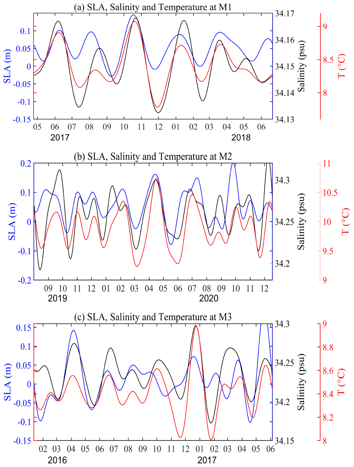
Figure 6 (a) The bandpass-filtered time series (20–120 d) of sea level anomalies (SLAs; blue curve), vertically averaged temperature (red curve), and salinity between 500–800 m (green curve) at station M1. (b) and (c) same as (a), but for M2 and M3. The filtering procedure was applied consistently to SLA, salinity, temperature time series prior to correlation analysis. Correlation coefficients were calculated using the filtered time series only, and only correlations significant at the 95 % confidence level (p<0.05) are reported in this study.

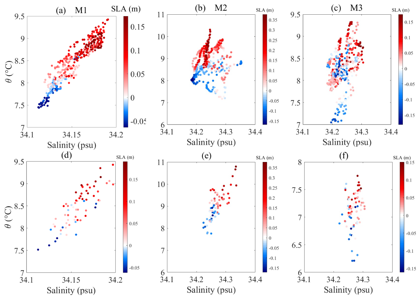
Figure 7 (a) The salinity and temperature data at M1 are displayed in a T–S scatter diagram with colors denoting the associated sea level anomalies (SLAs). (b) and (c) are same as (a), but for M2 and M3. (d), (e) and (f) are T-S plots of 500–800 m averaged temperature and salinity data from CMEMS product in the intermediate layer corresponding to the locations of M1, M2, and M3, respectively.

4 Disscussion

4.1 Structural Relationship Between Thickness and Salinity of NPIW

To further quantify the internal structure of the NPIW, linear regressions were performed between the thickness of the intermediate layer and the isopycnal-averaged salinity (between 26.4 and 26.9σ_θ) at the three mooring sites. The derived regression equations are as show in Fig. 8, where H represents the NPIW thickness (in meters) and salinity is the isopycnal-averaged salinity (in psu). The corresponding correlation coefficients between layer thickness and salinity are −0.63, −0.91, and −0.90 for M1, M2, and M3, respectively, indicating a strong and statistically significant inverse relationship at M2 and M3, and a weaker but still evident negative correlation at M1. All confidence intervals fall within the 95 % confidence level, confirming the statistical robustness of these relationships. The thickness–salinity relationship shown here is based on simultaneous daily observations and is intended to represent the overall structural covariability between the vertical extent of the low-salinity NPIW layer and its salinity characteristics, rather than a frequency-specific temporal correlation.

The relatively lower thickness–salinity correlation at M1 may be attributed to multiple factors. First, the NPIW core at M1 is located at greater depths, typically deeper than 600 m, and the salinity remained consistently below 34.2 psu throughout most of the observation period, exhibiting limited temporal variability. Such weak salinity fluctuations reduce the sensitivity of the thickness–salinity relationship and therefore weaken the linear correlation. In addition, because the lower 34.3 psu boundary was not continuously captured by the deepest CTD observations at M1, the NPIW thickness there was estimated using the 34.2 psu isohaline. This threshold lies closer to the low-salinity core, where the vertical salinity gradient is weaker, and may therefore be less sensitive to layer compression and expansion than the 34.3 psu boundary used at M2 and M3.

This weaker thickness–salinity correlation does not contradict the stronger SLA–salinity relationship at M1. SLA is used here as a surface indicator of mesoscale eddy activity, and the SLA–salinity correlation mainly reflects the linkage between eddy activity and intermediate-layer thermohaline variability. In contrast, the thickness–salinity correlation describes the structural covariability between the vertical extent of the low-salinity layer and its mean salinity. Thus, although M1 shows a relatively strong association between SLA and salinity, the salinity variations are not always accompanied by proportional changes in the thickness estimated from the 34.2 psu isohaline. Nevertheless, salinity and NPIW thickness at M1 still show a clear relationship, with thicker layers corresponding to lower salinity and thinner layers corresponding to higher salinity. In contrast, M2 and M3 are located in regions characterized by more dynamic water-mass interactions, including the influence of the Kuroshio, South China Sea Intermediate Water (SCSIW) (Mensah et al., 2015). The stronger thermohaline variability in these regions enhances the responsiveness of NPIW structure to salinity changes, thereby strengthening the statistical coupling between thickness and salinity.

These regression relationships reinforce the potential of using isopycnal-averaged salinity as a structural proxy for intermediate water thickness, especially in regions or datasets where direct thickness estimates are unavailable. This proxy relationship provides a valuable way for reconstructing historical thickness changes or interpreting reanalysis products in structural terms. More importantly, since mesoscale eddies actively modulate both salinity and vertical structure in the intermediate layer, the strong salinity–thickness coupling offers an indirect yet effective framework for linking eddy-induced thermohaline variability to volumetric changes in the NPIW.

Although the water mass structure at M2 and M3 is more complex, the enhanced salinity variability in these regions yields a more stable and robust relationship with NPIW thickness. This suggests that the intermediate water structure is highly sensitive to salinity perturbations and may respond coherently to mesoscale dynamical processes.

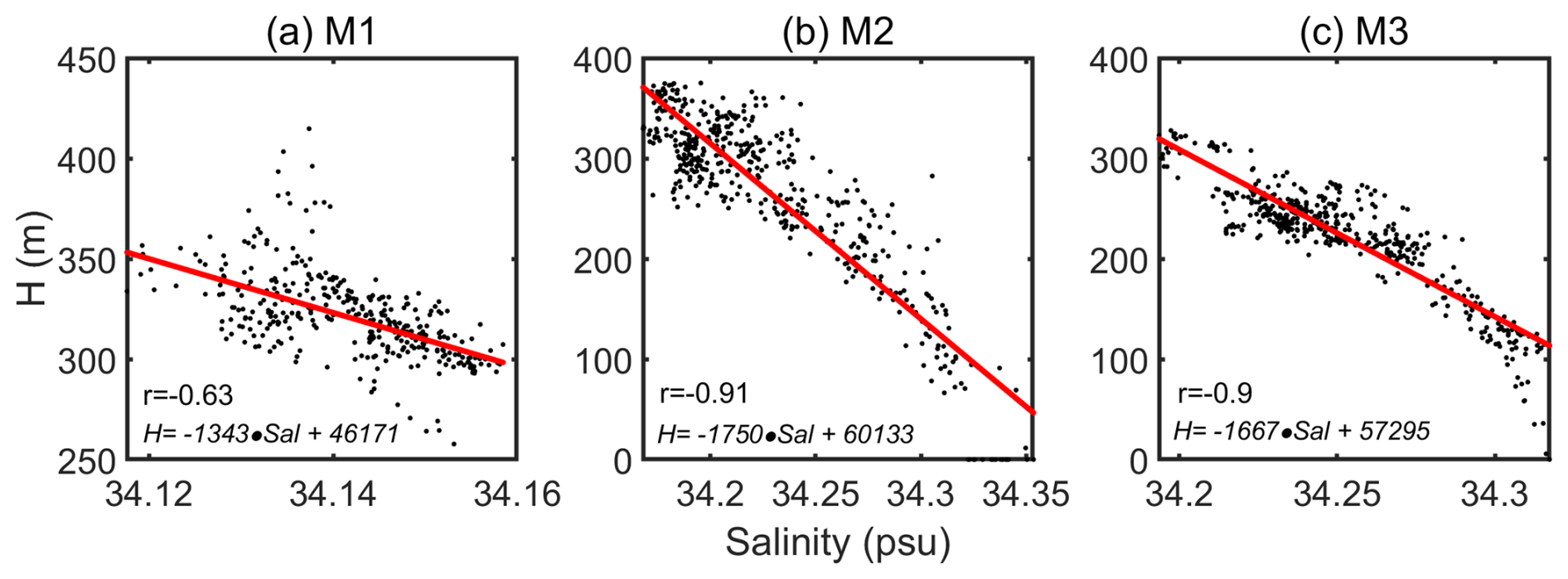
Figure 8 Scatterplots showing the relationship between NPIW layer thickness and isopycnal-averaged salinity (26.4–26.9σ_θ) at mooring sites M1, M2, and M3. Each point represents a daily-averaged value. Linear regression fits are shown in red line. The correlation coefficients are −0.63, −0.91, and −0.90 for M1, M2, and M3, respectively.

4.2 Eddy-associated Intraseasonal Variability of NPIW

The observed ∼ 80 d intraseasonal signal in sea level anomalies (SLA), consistently identified at moorings M1–M3, suggests that mesoscale variability may exert an important influence on NPIW properties. Wavelet analysis further reveals that SLA, salinity, and NPIW thickness variations share similar dominant periodicities within the 60–80 d band, which is broadly consistent with the typical timescales of westward-propagating mesoscale eddies reported in the western North Pacific (Qiu and Chen, 2005; Ren et al., 2020).

Time series analysis further demonstrates that the salinity within the isopycnal layer (26.4–26.9σ_θ) exhibits clear intraseasonal oscillations, which are strongly anti-correlated with variations in the thickness of the NPIW layer. This inverse relationship, with correlation coefficients exceeding −0.9 at M2 and M3, indicates that salinity is not only a tracer but also a reliable structural proxy for thickness variability in the intermediate layer. The westward propagation of SLA bands during eddy events was evident in longitude-time plots across all mooring latitudes (Fig. 9a, c, e), and lagged correlations between SLA and salinity (Fig. 9b, d, f) confirmed the 60–80 d propagation signals, with maximum correlation coefficients of 0.61, 0.5, and 0.6 at M1, M2, and M3, respectively. The observed eddy signatures were further supported by case analyses, in which anticyclonic (cyclonic) eddies were associated with increased (decreased) salinity and NPIW thickness.

To further illustrate these patterns, we selected characteristic events exhibiting significant salinity and temperature changes. At mooring M1, for instance, two representative events were identified: a high-salinity episode on 15 October 2017 (Event 1), and a low-salinity episode on 29 November 2017 (Event 2). Satellite observations during these periods revealed the presence of an anticyclonic eddy during Event 1 and a cyclonic eddy during Event 2 (Fig. 10a, b). At both M2 and M3, similar associations between eddy polarity and salinity/thickness anomalies were observed (Fig. 10c–f), reinforcing the notion that eddy polarity (cyclonic vs. anticyclonic) plays a significant role in driving both hydrographic and structural variability in the NPIW.

These results indicate that mesoscale eddies are a dominant source of intraseasonal variability in the intermediate layer, influencing both the hydrographic properties (salinity) and vertical structure (thickness) of the NPIW. The coupled response highlights the necessity of considering both parameters when diagnosing water mass evolution under eddy forcing.

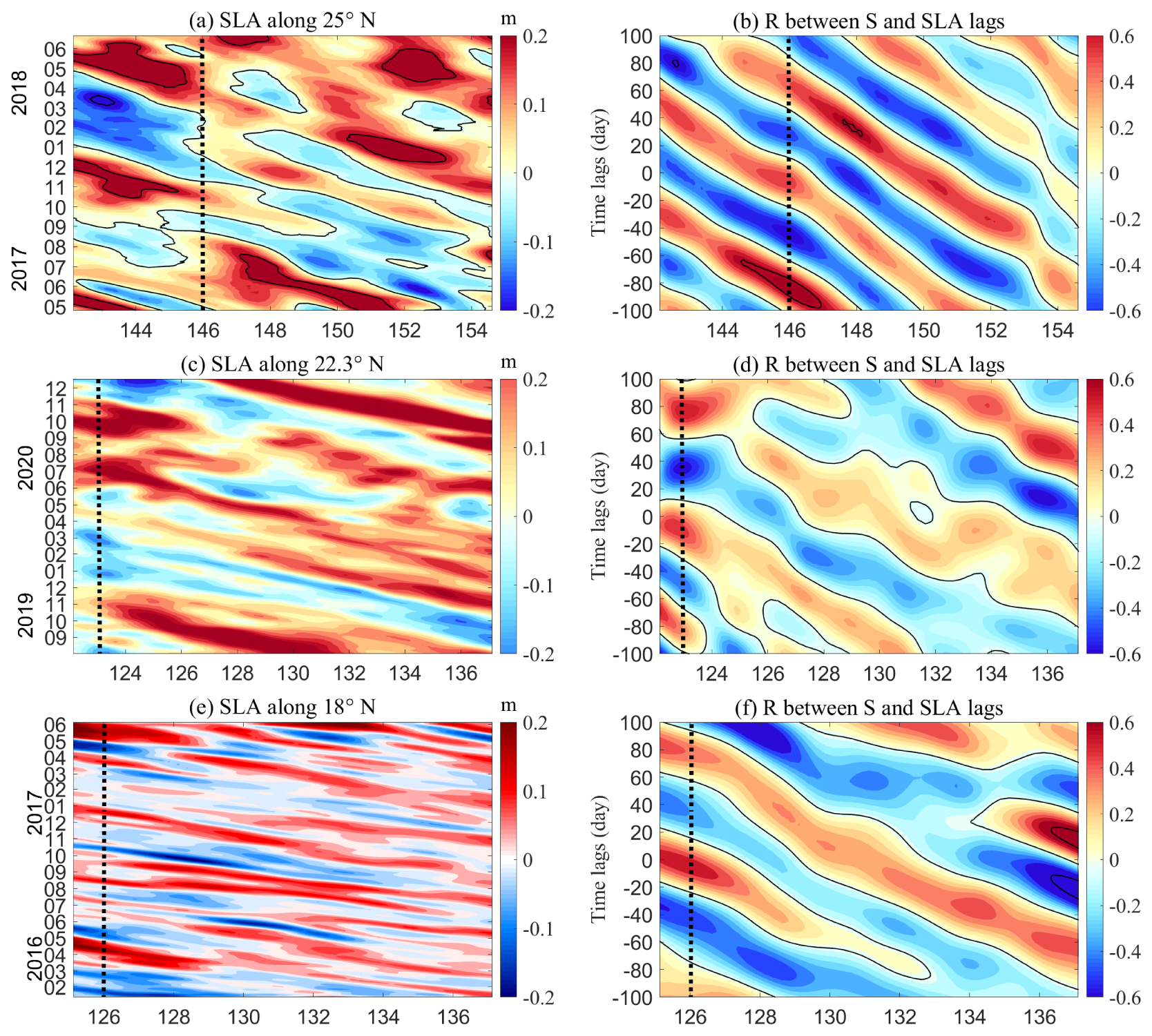
Figure 9 (a) Temporal evolution of sea level anomalies (SLAs) across longitudes at 25° N, as illustrated by the contour plots; (b) The correlation coefficient between salinity at M1 and SLA at different time lags, the vertical coordinates −100 to 100 d in (b) represent SLA lagging salinity for 100 d and SLA exceeding salinity for 100 d, respectively. (c) and (e) are same as (a), but its along 22.3° N and 18° N, respectively. (d) and (f) are same as (b), but for salinity from M2 and M3, respectively. Black contours in Fig. 9b, d, and f represent the zero isolines. The black dash line represent the location of M1, M2 and M3, respectively. The SLA data shown in this figure were obtained from the CMEMS dataset introduced in the Methods section.

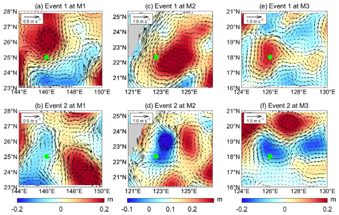
Figure 10 (a) and (b) are selected SLAs and surface geostrophic current maps corresponding to the moments of Event 1 and Event 2 observed from M1, respectively, where time of Event 1 corresponds to 15 October 2017 in Fig. 6a, and Event 2 corresponds to 29 November 2017 in Fig. 6a. (c) and (d) are same as (a) and (b), but for mooring site M2, where time of Event 1 and Event 2 at M2 corresponding to 20 April and 5 March 2020 showed in Fig. 6b. (e) and (f) are same as (a) and (b), but for mooring site M3, where time of Event 1 and Event 2 at M3 corresponding to 10 April 2016 and 15 April 2017 showed in Fig. 6c. The green dots denotes the mooring site, the colors shading represent the SLAs and the arrows indicate the surface geostrophic current.

4.3 Mechanisms of Structural Modulation of NPIW by Mesoscale Eddies

4.3.1 Evaluation of CMEMS and Intraseasonal Eddy Signals

Although the variations in temperature and salinity at several moorings are correlated with mesoscale eddies, it is challenging to understand from a broader perspective how mesoscale eddies influence temperature and salinity changes in intermediate layer at different regions. To further investigate the mechanisms by which mesoscale eddies modulate the intraseasonal variability of NPIW, we employed CMEMS reanalysis data as a complementary dataset to verify the robustness of our observational findings. Power spectral analyses of 500–800 m averaged salinity at the mooring locations (Fig. 11a–c) revealed significant intraseasonal signals with dominant periods of 60–80 d, consistent with those derived from mooring data. This confirms that the intraseasonal variability of salinity in the intermediate layer is a robust signal and is well captured by both in situ observations and reanalysis data. Furthermore, we compared scatter plots of SLA against temperature and salinity derived from both mooring observations (Fig. 8a–c) and CMEMS reanalysis data (Fig. 8d–f). The CMEMS results exhibit similar positive correlations between SLA and temperature/salinity, reinforcing the reliability of the dataset for representing the hydrographic properties and eddy-induced variations in NPIW.

To quantitatively evaluate the ability of CMEMS to represent intermediate-layer salinity variability, we compared the salinity amplitude and standard deviation between CMEMS and the mooring observations at M2 and M3. Here, the salinity amplitude is defined as the difference between the maximum and minimum salinity at each depth, whereas the standard deviation describes the temporal variability around the mean state. The corresponding CMEMS-derived max standard deviations are 0.04 psu at M2 and 0.04 psu at M3. At M2, the CMEMS-derived salinity amplitude ranges from 0.10 to 0.22 psu, which is smaller than the mooring-derived amplitude of 0.15–0.30 psu. At M3, the CMEMS-derived amplitude ranges from 0.09 to 0.17 psu, generally comparable to the mooring-derived amplitude of 0.05–0.25 psu. These results indicate that CMEMS reproduces the observed intermediate-layer salinity variability at the same order of magnitude, although it tends to underestimate the amplitude at M2. This underestimation may be related to the 7 d temporal resolution of CMEMS and the smoothing effect of gridded reanalysis products. Therefore, its representation of the intraseasonal signals and variability amplitudes provides useful support for the subsequent analysis of the spatial structure and eddy-related mechanisms.

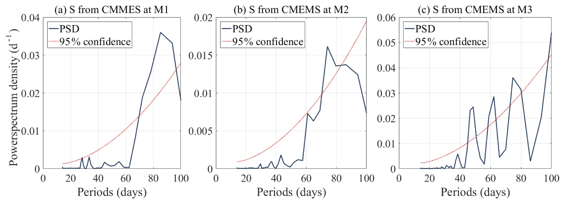
Figure 11 (a) The power spectrum density of 500–800 m averaged salinity at location of M1 from CMEMS data. (b) and (c) are same as (a), but for location of M2 and M3, respectively. The red dash line represent the 95 % confidence level.

4.3.2 Horizontal and Vertical Responses of NPIW to Mesoscale Eddies

To further illustrate the spatial structure, we used CMEMS data to calculate the horizontal distributions of salinity and NPIW thickness. The anticyclonic eddy (AE) and cyclonic eddy (CE) events shown in Figs. 12 to 14 were identified based on the sign of the SLA near each mooring station, with positive SLA corresponding to AE conditions and negative SLA corresponding to CE conditions. A composite field was constructed by averaging all identified AE and CE events at each station. The thickness was defined as the vertical distance between the upper and lower boundaries of the 34.3 psu isohaline, representing the volumetric extent of the low-salinity core. Figures 12 to 14 present the composite spatial distributions of intermediate-layer salinity and NPIW thickness at the three mooring sites. These maps demonstrate that mesoscale eddies not only modify the thermohaline characteristics of the NPIW but also significantly reshape its vertical structure. It should be noted that the salinity variations discussed here mainly represent changes within a fixed-depth intermediate layer, rather than intrinsic properties of the eddy cores themselves. Under anticyclonic eddy conditions associated with positive SLA, the intermediate-layer isopycnals are generally displaced downward, compressing the low-salinity NPIW layer and increasing the relative contribution of surrounding higher-salinity waters within the observed depth range. As a result, anticyclonic eddies are associated with relatively elevated salinity and reduced NPIW thickness. In contrast, cyclonic eddies induce upward displacement of isopycnals and expansion of the low-salinity layer, which helps preserve the fresher characteristics of the NPIW and results in a thicker intermediate layer. The spatial distribution of layer thickness differs notably among M1–M3, consistent with the mooring-derived thickness variations, where M1 exhibits a generally thicker intermediate layer than the other sites. This spatial correspondence aligns with the strong inverse correlation between salinity and thickness identified in the time series, further confirming that layer thickness also as an effective indicator of the eddy-induced modulation of NPIW structure.

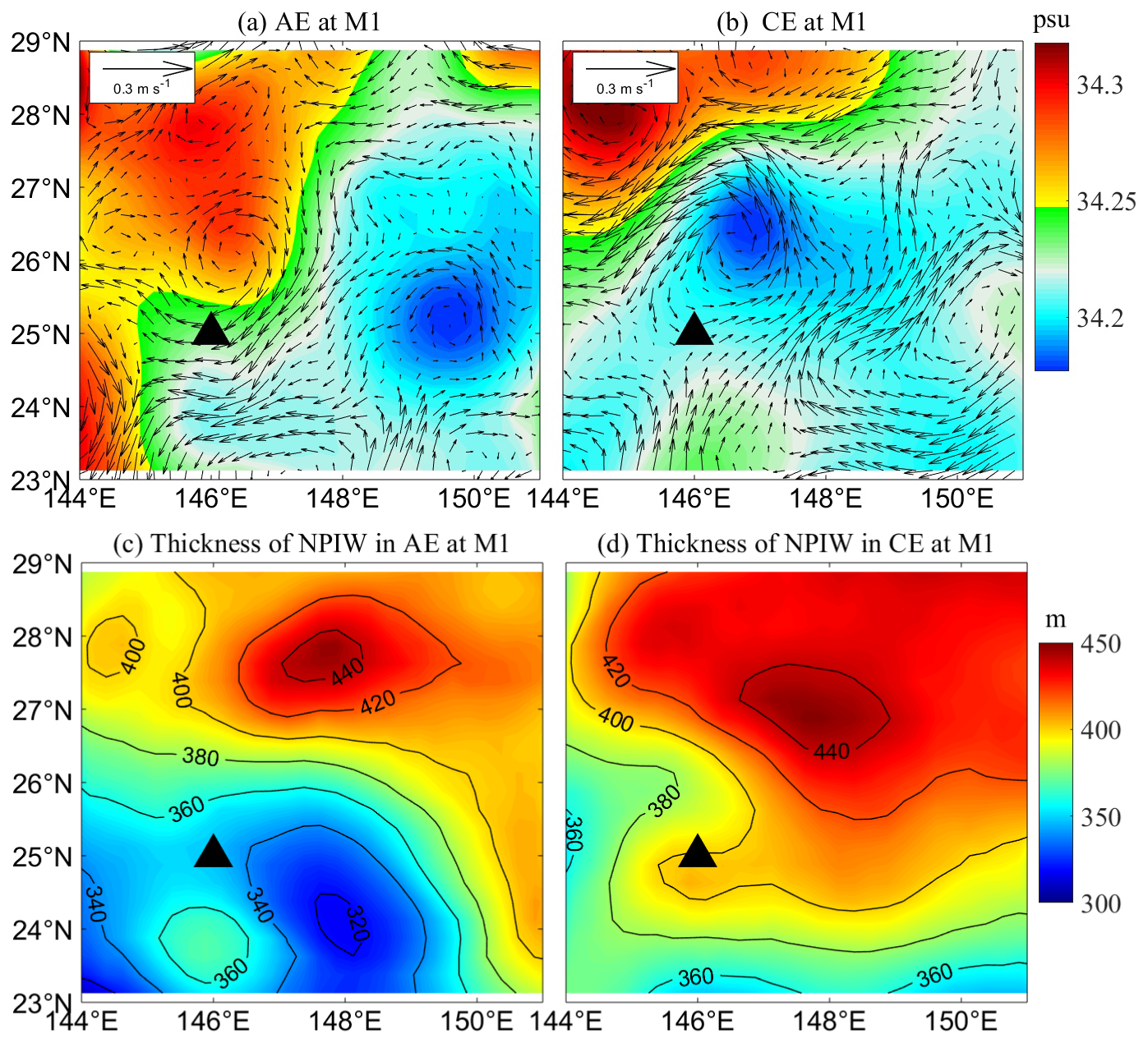
Figure 12 (a) Composite distribution of salinity (color shading) and current vectors (black arrows) averaged over the 500–800 m layer during high-salinity events generally associated with anticyclonic conditions near the M1 mooring site form CMEMS data. (b) Same as (a), but for low-salinity events generally associated with cyclonic conditions. (c) Composite thickness of the NPIW layer during high-salinity events, calculated from the 34.3 psu isohaline boundaries. (d) Same as (c), but for low-salinity events. Black triangles indicate the mooring locations.

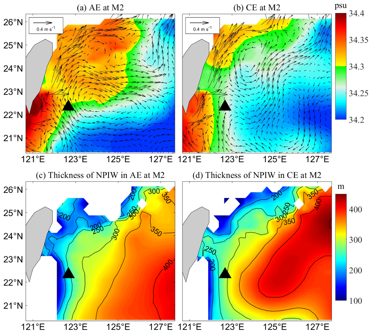
Figure 13 (a) Composite distribution of salinity (color shading) and current vectors (black arrows) averaged over the 500–800 m layer during high-salinity events generally associated with anticyclonic conditions near the M2 mooring site form CMEMS data. (b) Same as (a), but for low-salinity events generally associated with cyclonic conditions. (c) Composite thickness of the NPIW layer during high-salinity events, calculated from the 34.3 psu isohaline boundaries. (d) Same as (c), but for low-salinity events. Black triangles indicate the mooring locations.

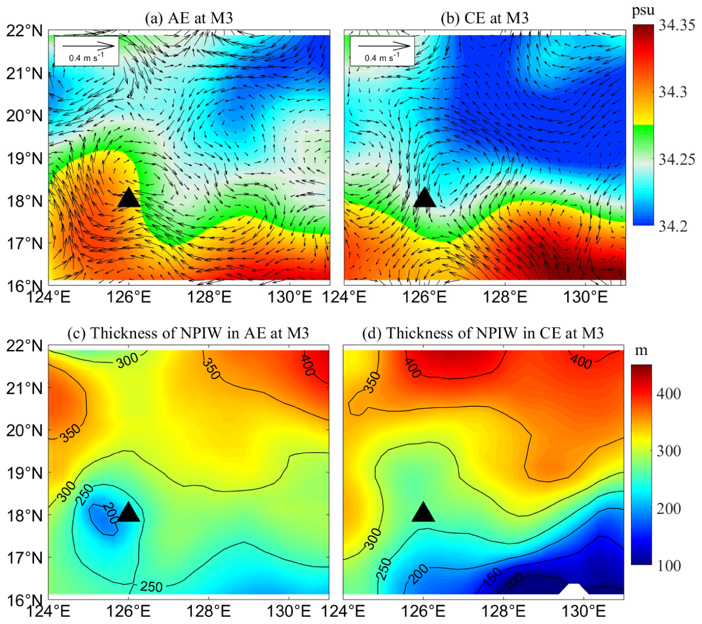
Figure 14 (a) Composite distribution of salinity (color shading) and current vectors (black arrows) averaged over the 500–700 m layer during high-salinity events generally associated with anticyclonic conditions near the M3 mooring site form CMEMS data. (b) Same as (a), but for low-salinity events generally associated with cyclonic conditions. (c) Composite thickness of the NPIW layer during high-salinity events, calculated from the 34.3 psu isohaline boundaries. (d) Same as (c), but for low-salinity events. Black triangles indicate the mooring locations.

To further examine the three-dimensional structure of the eddy-related NPIW response, CMEMS-based composite vertical sections of temperature and salinity were constructed along the M2 transect under anticyclonic and cyclonic eddy conditions (Fig. 15). The sections show clear differences in the vertical structure of the intermediate layer between the two eddy states. During anticyclonic eddy conditions, the intermediate-layer isopycnals are displaced downward, and the 34.3 psu isohaline encloses a relatively thinner low-salinity layer near the M2 mooring. This compressed structure is accompanied by higher salinity within the intermediate layer, especially on the western side of the section. This feature is consistent with the horizontal salinity composite, which shows a high-salinity band extending toward the M2 region. Therefore, the elevated salinity at M2 may be associated not only with vertical compression of the low-salinity NPIW layer, but also with lateral redistribution of surrounding higher-salinity intermediate waters, possibly related to regional water-mass exchange involving the South China Sea Intermediate Water (SCSIW). In contrast, during cyclonic eddy conditions, the 34.3 psu isohaline extends over a thicker vertical range near M2, indicating expansion of the low-salinity NPIW layer, with relatively lower salinity. These vertical composite structures provide additional evidence that the inverse relationship between NPIW thickness and salinity is closely related to eddy-induced vertical displacement and compression or expansion of the intermediate low-salinity layer. Similar vertical compression and expansion characteristics are also found at the other mooring sites, but M2 is shown here as a representative example because the western-boundary water-mass interaction is most evident at this site.

The modulation of NPIW by mesoscale eddies exhibits clear spatial heterogeneity among the three sites. At M1, the intermediate water responds relatively weakly to anticyclonic eddies, showing smaller salinity variations. This weaker response is primarily attributed to the deeper position of the NPIW core at this site, where anticyclonic eddies mainly induce vertical displacement of isopycnals. Owing to the absence of nearby high-salinity water sources, the resulting thermohaline changes remain relatively limited. Nevertheless, the observed downward displacement of isopycnals during anticyclonic periods still indicates a clear vertical adjustment of the intermediate layer, suggesting that mesoscale eddies participate in the structural evolution of the NPIW in a relatively stable.

In contrast, the M2 and M3 sites near the western boundary exhibit much stronger salinity and thickness variability. Compared with M1, these regions are influenced by more complex intermediate-water interactions involving the SCSIW, Kuroshio Intermediate Water (KIW), and saline subtropical waters from the western tropical Pacific. Such a background favors stronger lateral exchange and water-mass redistribution. Under anticyclonic eddy conditions, the downward displacement of isopycnals compresses the low-salinity NPIW layer, while the surrounding higher-salinity waters may be laterally redistributed into the intermediate layer, particularly near the western boundary. As a result, the NPIW at M2 and M3 tends to exhibit elevated salinity and reduced thickness, with a temporarily weakened low-salinity signature. These features suggest that mesoscale eddies near the western boundary modulate the NPIW through both vertical compression and lateral water-mass redistribution. At M2, the composite thickness field does not exhibit a well-defined eddy-like structure as clearly as at the other sites. This may be related to the complex dynamical environment east of Taiwan, where westward-propagating mesoscale eddies interact strongly with the Kuroshio and the western boundary circulation. Previous studies have shown that such eddy–Kuroshio interactions can deform, weaken, or reorganize mesoscale eddy structures in this region (Zhang et al., 2001; Yin et al., 2017). As a result, the composite horizontal structure may not retain an idealized cyclonic or anticyclonic eddy pattern in Fig. 13. Nevertheless, significant differences in NPIW thickness and salinity are still observed between the two composite states, indicating that mesoscale variability continues to modulate the intermediate-water structure in this region.

Although the present results suggest a close association between mesoscale eddies and the observed intraseasonal variability of the NPIW, other processes may also contribute to variability on similar timescales. For example, remotely forced baroclinic Rossby waves may influence sea level and subsurface isopycnal displacement in the western North Pacific. However, the coherent variability observed among SLA, salinity, and NPIW thickness, together with the contrasting responses under anticyclonic and cyclonic conditions, suggests that mesoscale variability is likely the dominant contributor in the present observations. Overall, these results suggest that mesoscale eddies modulate the NPIW through both vertical isopycnal displacement and lateral water-mass redistribution. The former mainly controls the compression and expansion of the low-salinity NPIW layer, whereas the latter may further enhance salinity anomalies near the western boundary, particularly at M2 and M3. At M1, the weaker salinity anomalies indicate a relatively stronger role of vertical displacement, while the more complex hydrographic background near M2 and M3 favors additional lateral exchange of surrounding higher-salinity intermediate waters.

It should be noted that the three mooring observations analyzed in this study do not fully represent the entire North Pacific basin. Instead, the moorings were strategically deployed across different hydrographic environments in the western North Pacific, including the open-ocean NPIW core region and the western boundary mixing region. In addition, the three mooring records were obtained during different periods, with M3 during 2016–2017, M1 during 2017–2018, and M2 during 2019–2020. Therefore, the differences among the three mooring sites should not be interpreted as purely spatial contrasts. Interannual variability in the background hydrographic state, regional eddy activity, and large-scale circulation may also contribute to the observed site-to-site differences. Previous studies have shown that the salinity minimum of the NPIW, water-mass properties in the western North Pacific, and eddy activity in the Kuroshio Extension region can vary on interannual to decadal timescales.

Nevertheless, the main focus of this study is the intraseasonal variability within each mooring record and its relationship with mesoscale eddy signals. The inverse relationship between NPIW thickness and salinity, together with the coherent association among SLA, salinity, and thickness at individual sites, remains evident within each observational period. Therefore, the non-overlapping observation periods do not alter the conclusion that mesoscale eddies modulate the NPIW structure, but they do imply that the cross-site comparison reflects both regional hydrographic differences and possible interannual modulation. This limitation has been considered in the interpretation of the spatial heterogeneity discussed above.

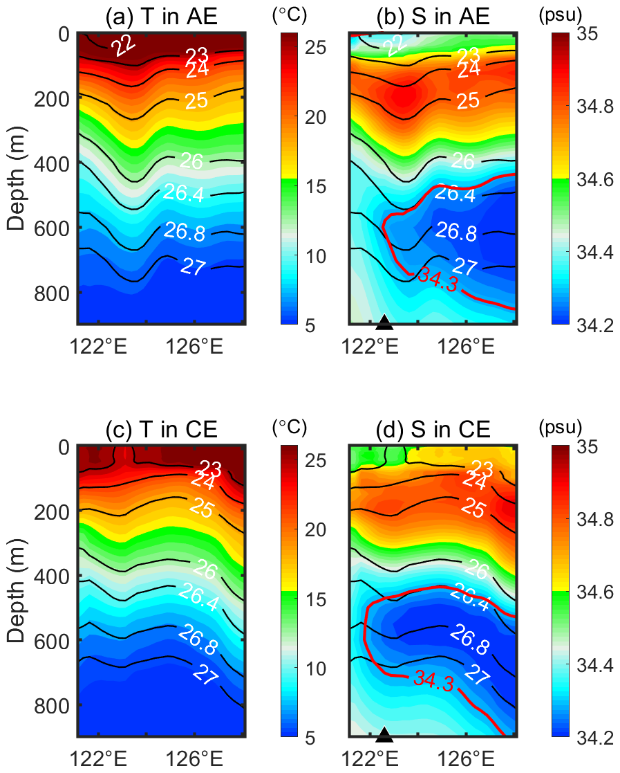
Figure 15 Composite vertical sections of temperature and salinity along the M2 transect during anticyclonic and cyclonic eddy form CMEMS data. (a, b) Temperature and salinity sections during anticyclonic eddy, respectively. (c, d) Same as (a, b), but for cyclonic eddy. Color shading represents temperature in (a), (c) and salinity in (b), (d). Black contours indicate potential density, and red contours in (b), (d) denote the 34.3 psu isohaline. The black triangle indicates the location of the M2 mooring.

5 Conclusions

This study based on three long-term mooring observations (M1–M3) and reanalysis data in the western Pacific, systematically investigates the intraseasonal variability of the NPIW and its modulation by mesoscale eddies. Wavelet analysis reveals a consistent ∼ 80 d periodicity across all sites, and satellite altimetry confirms that these intraseasonal signals are primarily induced by westward-propagating mesoscale eddies.

A major innovation of this study is the introduction of NPIW layer thickness as a structural diagnostic index, it quantitatively characterizes the compression and expansion of the NPIW under eddy forcing. All three moorings show a strong inverse correlation between layer thickness and salinity, indicating a tight coupling between thermohaline anomalies and structural variations. This new metric provides a more comprehensive framework for describing NPIW evolution beyond temperature–salinity anomalies alone.

Composite maps further show that anticyclonic eddies correspond to higher salinity and thinner intermediate layers, whereas cyclonic eddies produce lower salinity and thicker layers. This spatial coherence highlights the role of eddy-induced vertical compression and uplift in modulating NPIW structure. In the core of NPIW region, the eddy impact is mainly vertical and moderate, while in the western boundary region, where multiple water masses (SCSIW, KIW) interact, stronger eddies not only alter NPIW thickness but also introduce high-salinity waters through horizontal advection and mixing, occasionally leading to the weakening of the low-salinity NPIW signature.

In summary, by integrating multi-site observations with a new structural diagnostic approach, this study reveals how mesoscale eddies control the structure and property variability of NPIW. The inclusion of layer thickness provides a novel and physically grounded perspective, extending beyond previous single-site analyses and enhancing our understanding of intermediate-water dynamics in the western Pacific.